SR-CLD: spatially-resolved chord length distributions for statistical description, visualization, and alignment of non-uniform microstructures

Abstract

This study introduces the calculation of spatially-resolved chord length distribution (SR-CLD) as an efficient approach for quantifying and visualizing non-uniform microstructures in heterogeneous materials. SR-CLD enables detailed analysis of spatial variation of microstructure constituent sizes in different directions that can be overlooked with traditional descriptions. We present the calculation of SR-CLD using efficient scan-line algorithm that counts pixels in constituents along pixel rows or columns of microstructure images for detailed, high-resolution SR-CLD maps. We demonstrate the application of SR-CLD in two case studies: one on synthetic polycrystalline microstructures with known and intentionally created uniform and gradient spatial distributions of grain size; and one on experimental images of two-phase microstructures of additively manufactured Ti alloys with significant spatially non-uniform distributions of laths of one of the phases. Additionally, we present how SR-CLDs can enable automated, computationally efficient, and robust alignment of large sets of images for merging into accurate composite images of large microstructure areas.

1 Introduction

Process–microstructure–property relationships of materials serve as the cornerstone of materials science and engineering. Efficient materials design requires not only qualitative but also quantitative understanding of these relationships. Quantitative process–microstructure–property relationships require rigorous description of the materials microstructure. Rigorous quantitative description of microstructures is not trivial, especially in structural metals and alloys that have a rich variety of microstructure constituents of interest at multiple length scales [1]. In many structural alloys, phases and grains are the constituents of special interest as they play a decisive role in a suite of engineering properties (e.g., stiffness, strength, fatigue, toughness) [2].

Microstructures are typically described by the statistics of size metrics of constituents such as areas, equivalent diameters, and intercepts (chords). Areas are often considered in microstructure maps where individual constituents can be clearly isolated: e.g., electron back-scattered diffraction (EBSD) maps [3] or segmented optical/electron microscopy images. It is common practice to convert areas of constituents (especially grains) into equivalent diameters, e.g., diameters of circles of the same area as the constituent [4]. The equivalent diameter is often a more preferred geometric descriptor than the area even for irregularly shaped grains because it is intuitive and compatible with widely used property models, e.g., the Hall–Petch model relating the yield strength to the average grain diameter of polycrystalline metals and alloys [5, 6]. For significantly non-equiaxed microstructures (e.g., in rolled alloys with elongated grains), equivalent ellipses can be considered instead of circles [7, 8]. The ellipse representation allows analyzing distributions of major and minor diameters as well as aspect ratios and inclination angles of the major axes [9], which provides insights into not only size but also, to some extent, morphology of the constituents and their geometric orientations.

The intercept, or chord, is another size metric used in statistical microstructure analysis for both equiaxed and non-equiaxed constituents. A chord is a line segment completely contained within a microstructure constituent (see $l_{i}$ in Figure 1a). The advantage of the chord is that it can be defined and measured for constituents with arbitrarily complex shapes without the underlying approximation to a circle, ellipse, or any other idealized shape. Chords are further advantageous in the context of microstructure–property relationships because chord lengths are directly relevant to transport properties in heterogeneous materials [10, 11] and properties dictated by free paths in the microstructure, e.g., slip resistance related to the dislocation free path between grain boundaries [12, 13, 14].

In standardized practice, chords are sampled using test lines or other simple test objects (e.g., circles) [15]. To this end, one randomly overlays test lines (circles, or other objects) with the microstructure map and then identifies intersections with the boundaries of the constituents of interest. Chord lengths can be then estimated from the number of intersections per test line of a known length [15]. Upon sampling, the mean chord length value can be obtained and reported either directly or, in the case of grain size analysis, converted to an average size using standardized tables [15]. Some aspects of these standardized protocols of chord length analysis arise from the historical origins of manual measurements in non-digital micrographs.

The emergence of modern tools of image processing, computational statistics, and visualization, as well as a shift towards digital microstructure data obtained by most of the current characterization instruments give rise to not only automation of measurements but also new, more detailed approaches to microstructure analysis. First of all, for digital microstructures, chord lengths can be calculated directly, rather than estimated from a number of intersection points. Second, automated and direct calculation allows obtaining chord lengths from a large number of test lines overlaid with the microstructure, as opposed to sampling with a few random test lines. The advantage is that systematic sampling with numerous parallel lines allows resolving the chord lengths and their distributions in different directions. For example, Lehto et al. [16, 17] presented a local grain size analysis method that calculates chord lengths in four directions ($0\mathrm{°}$, $45\mathrm{°}$, $90\mathrm{°}$, and $135\mathrm{°}$) for each point in polycrystalline microstructures of welded steel. Latypov et al. [18] presented high-resolution angularly-resolved chord length distributions (CLDs) for EBSD grain maps of polycrystals . Turner et al. [19] developed a computational method of calculation of directional CLDs for 3D voxelized microstructures.

Literature inspection shows that standardized and commonly used protocols of microstructure analysis focus on statistical summaries of size metrics (e.g., mean values) that assume idealized shapes (e.g., equivalent diameters) or calculated using methods grounded to originally manual measurements (e.g., number of intercepts with random test lines). A shift towards digital microstructure quantification shows the potential for more systematic and granular analyses with automated computational approaches, as seen in advances in resolving the chord lengths and their distributions in different directions [18, 20, 21]. Yet, even with recent advances, the existing approaches overlook spatial variation of size distributions of the constituents, which is only adequate for materials with spatially uniform microstructures. In this context, there is a growing need for new methods that can account for spatial variations. The need comes from the emergence of new classes of materials with intentionally designed non-uniform microstructures (e.g., heterostructured [22], architectured [23], gradient [24], or lithomimetic [25] materials) and the corresponding new (as well as conventional) processing methods (friction stir welding [26], additive manufacturing [27], severe plastic deformation [28]). Related work in this direction includes the calculation of moving averages of the grain size [29] or the second-phase particle thickness [30] along principal directions in the microstructure. Building on the prior work of moving averages and directionally resolved CLDs, we present a method of the calculation and visualization of high-resolution spatially-resolved chord length distribution (SR-CLD). Our method is developed to capture spatial variations of the constituent size distributions along selected directions in diverse types of microstructures. In Section 2, we describe the details of our SR-CLD method and then demonstrate its use in case studies in Section 3.

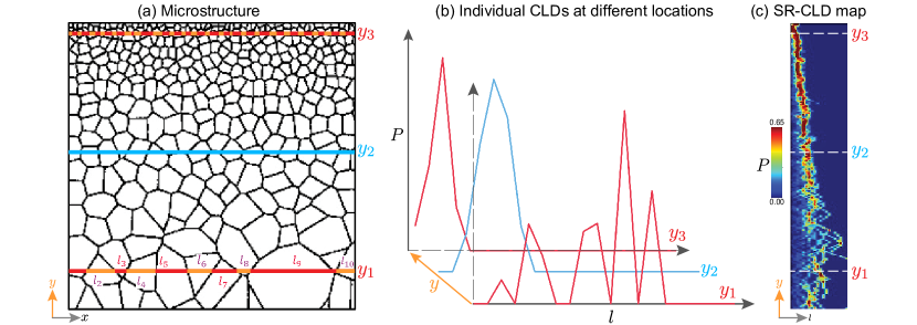
Figure 1: Illustration of the SR-CLD calculation: (a) a polycrystalline microstructure with overlaid horizontal chords obtained for selected vertical locations; (b) distributions of horizontal chords (CLDs) calculated at three locations along the $y$ axis; (c) SR-CLD map that can be thought of as a stack of individual CLDs with the probability, $P$, represented by color.

2 Spatially-resolved chord length distributions

For calculation of individual chord lengths, we adopt the scan-line method proposed by Turner et al. [31]. The method is suitable for digital microstructures defined on (pixel) grids, where microstructure constituents have pixel labels distinct from either boundaries or neighboring constituents. Given a grid of pixel values uniquely defining constituents of interest, we calculate horizontal (vertical) chord lengths by iterative pixel count for every row (column) of pixels on the microstructure grid. Consider the calculation of horizontal chord lengths in an example microstructure shown in Figure 1(a). For every row, starting from one end, we count pixels inside a microstructure constituent with the same label in a continuous stretch. While scanning pixels along the row, every time a new label or a boundary is encountered, we stop the pixel count, record the chord length (in pixels), and then restart the pixel count for the next constituent. We repeat the calculation for every row in the image and collect row-specific chord length datasets. For each dataset, we then bin the chord lengths and calculate row-specific (horizontal) distributions as shown with a couple of scan lines in Figure 1(b). If the microstructure map has $K$ rows, the procedure would result in $K$ sets of chord lengths and $K$ CLDs. The calculation of chord lengths and their distributions in the vertical direction is identical to that for horizontal CLDs with the only difference being that pixels are scanned vertically along pixel columns instead of rows.

We represent row- or column-specific distributions (SR-CLDs) by probabilities, $P_{i}^{(k)}$, of finding a chord length within a small interval centered at a discrete value, $l_{i}$, in a $k$th row or column of the microstructure calculated as follows:

$$P_{i}^{(k)}=\cfrac{N_{i}^{(k)}l_{i}}{\displaystyle\sum^{B}_{i=1}N_{i}^{(k)}l_{i}},$$ (1)

where the index $i$ enumerates bins from $1$ to $B$, $N_{i}$ denotes the number of chords within the interval of the $i$th bin with its center corresponding to the chord length $l_{i}$.

The described calculation results in SR-CLDs numerically represented by two-dimensional probability arrays (matrices) of size $K\times B$. For intuitive interpretation of SR-CLDs, we propose a visualization of SR-CLD arrays as heat maps, where one axis represents the spatial coordinate (along which the spatial variation of CLDs is captured), the other axis represents the chord length, and the color depicts the CLD probability. Such heat maps can be thought of as CLDs sequentially calculated across a microstructure, stacked together along a spatial axis with the probability axis represented by color (Figure 1(c)). As seen in the simple example in Figure 2 and in subsequent case studies, such visualization of SR-CLDs allows quick and intuitive visual assessment of the spatial uniformity (or lack thereof) in the microstructure in terms of constituent sizes.

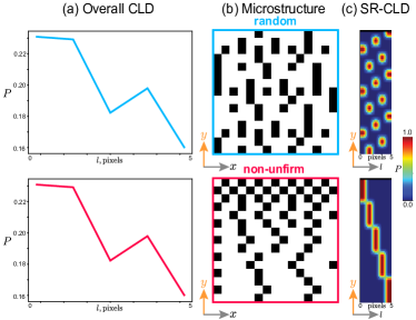
Figure 2: Illustration how (a) overall size distributions (here, overall CLDs) can be identical for (b) two very different microstructures: (i) one with random spatial distribution of a constituent of interest (white pixels), (ii) one with non-uniform, gradient variation of the volume fraction of the constituent; and how (c) SR-CLD can capture such differences in microstructures.

Note that, if the chord lengths are calculated and aggregated into a single dataset from all pixel rows or columns, the calculation would result in an overall CLD for a given direction, as considered in previous studies [19, 18]. Figure 2 illustrates advantages of SR-CLDs compared to overall CLDs. Overall CLDs calculated in the horizontal direction for two synthetic microstructures are identical although the microstructures are clearly different with one being non-uniform (Figure 2(a)). It is the consideration of chord lengths along individual rows/columns followed by row-/column-wise calculation of distributions that spatially resolves the CLD to capture the spatial variation of microstructure constituents as seen in Figure 2(c). Mathematically, the spatial resolution of CLDs is signified by the index $k$ that enumerates rows for horizontal CLDs or columns for vertical CLDs. In this study, we discuss the calculation and analysis of SR-CLDs along two principal directions (horizontal and vertical), however, this method can be generalized to any direction in a microstructure.

The SR-CLD values in the numerical arrays and their corresponding heat map visualizations depend on the binning of chord lengths selected in the CLD calculation (Equation 1). The choice of the binning, and specifically the number of bins for calculating a distribution is not trivial; and much research has been dedicated on determining the optimal number of bins that convey a representative distribution of a given dataset [32, 33, 34, 35, 36]. Some common methods of determining the number of bins include the square root rule, Sturges’ formula [32], Scott’s normal reference rule [33], Freedman–Diaconis Rule [34], Rice’s rule [35], and Doane’s formula [36]. In this work, we explored all these methods and chose Doane’s formula for SR-CLD calculations due to the large number of chords and skewness of the distribution present in most considered cases.

3 Case studies

We demonstrate the application of our methodology in two case studies: (i) synthetic polycrystalline microstructures and (ii) experimental two-phase microstructures. The first case study serves as a proof of concept in which SR-CLD describes a known and intentionally created gradient in the grain size in synthetically generated polycrystals. The second case study analyzes non-uniform microstructures experimentally obtained in additively manufactured Ti alloys. Beyond these case studies, we present an additional application of SR-CLD for efficient and effective automated alignment of a large number of microstructure images.

3.1 Synthetic polycrystalline microstructures

To evaluate the SR-CLD approach on a microstructure with known non-uniform spatial distributions of the constituent size, we generated synthetic 2D polycrystals using the open-source software Neper [37, 38]. We generated two representative polycrystals (Figure 3(a)): (i) a polycrystal with uniform grain size and (ii) a polycrystal with a monotonically decreasing grain size along the vertical direction (the $y$ axis in Figure 3). To this end, we used different settings of grain seeding available in Neper: random for the uniform polycrystal and biased for the polycrystal with a grain size gradient. The biased seeding aimed for a $300\text{\,}\mathrm{\char 37\relax}$ increase in grain size from top to bottom ends of the microstructure. Both polycrystals contained 1108 grains and similar overall grain size distribution and mean grain size (Figure 3(c,d)).

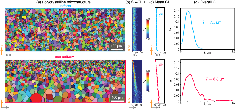
Figure 3: Description of (a) two polycrystalline microstructures with a uniform and non-uniform (gradient) distribution of grain size using (b) SR-CLD; (c) spatially resolved mean chord length (CL), (d) overall (non-spatially-resolved) CLD.

To quantitatively compare spatial variations in these polycrystals using the SR-CLD approach, we worked with binary images of the polycrystals exported from Neper. In the binary images of pixel size $284\times 786$, grain interiors were represented with white and grain boundaries with black pixels. By counting uninterrupted stretches of white pixels in each row, we digitally measured horizontal chords and computed $K=284$ chord length distributions (CLDs) for all of 284 pixel rows using Equation 1 with $B=39$ bins, as determined from Doane’s formula. Figure 3(b) displays the results of this SR-CLD calculation visualized as heat maps.

The SR-CLD clearly captures the gradient in the grain size when it is present: the SR-CLD for the gradient polycrystal shows a shift of the prevalent chord length from about 4 to $18\text{\,}\mathrm{\SIUnitSymbolMicro m}$ (Figure 3(b)). This trend is confirmed with the moving average chord length also shown in Figure 3(c) alongside the SR-CLD maps. Unlike the mean chord length however, the SR-CLD map additionally shows the variance in the chord lengths for each vertical location. The top part of the microstructure has small grains of consistent size, as seen from a high probability in the narrow range of chord lengths (red bands in the SR-CLD map, Figure 3(b)). On the other hand, the probability is lower and spread over a wider range of chord lengths for the bottom part of the gradient microstructure containing large grains with a greater variety of horizontal chord lengths. In contrast to the gradient polycrystal, the microstructure generated with random seeding is characterized by a consistent mean chord length (Figure 3(c)) and a SR-CLD with no trend: the chord length probability is in a consistent range centered around $9\text{\,}\mathrm{\SIUnitSymbolMicro m}$ (Figure 3(b)).

3.2 Two-phase microstructures of titanium alloys

The second case study demonstrates the application of SR-CLD on real microstructures to describe spatial variation of phase sizes. Specifically, we quantify the spatial variation of the $\alpha$ phase in two-phase microstructures of two dissimilar titanium alloys additively manufactured and experimentally characterized by Kennedy et al. [30]. The authors co-deposited Ti5553 and Ti64 alloys using a wire-arc additive manufacturing process, which results in spatial variations of the composition, microstructure, and thus properties (e.g., strength and damage tolerance). The spatial microstructure variation is primarily manifested in a variation of the lath size of the $\alpha$ phase. To demonstrate our approach for these materials, we processed the raw experimental images of the phases into the binary format consistent with the pixel count method, aligned the individual images into large composite images and calculated SR-CLD for the entire composite images.

Raw data and image pre-processing. Raw data published by Kennedy et al. [30] contain over 900 high-resolution scanning electron microscope images for two additively manufactured materials: Ti5553-on-Ti64 and Ti64-on-Ti5553. To segment the raw images, we first applied a Gaussian filter (with radius of $5\text{\,}\mathrm{p}\mathrm{x}$) and then applied a threshold optimally selected using Yen’s method [39] to obtain binary images whose white pixels represent the $\alpha$ phase (laths) of interest. The binary images were passed through erosion and dilation filters to clean up the remaining segmentation noise [40, 41]. Hundreds of the individual segmented images were then aligned and merged into large composite images: one for Ti5553-on-Ti64 and one for Ti64-on-Ti5553 samples (except a couple of stained images at the top of the analyzed regions).

SR-CLD calculation. We calculated SR-CLDs for both composite images despite their very large size ($288688\times 3897$ each) following merging. Horizontal chord lengths were measured for the $\alpha$ phase by counting the corresponding white pixels at each pixel row. From the measured chord lengths, we estimated $288\,688\text{\,}$ CLDs using Equation 1 with $B=55$ bins, also for all $288\,688\text{\,}$ pixel rows. While we obtained the SR-CLD maps for the entire composite images, they are so large that we can practically present the results only for microstructure subregions of approximately $70\text{\,}\mathrm{\SIUnitSymbolMicro m}$ along the $y$ axis – the direction of the microstructure variation (Figure 4). Figure 4 shows two subregions of each processed microstructure and their corresponding SR-CLD maps and moving average chord length curves for the two studied materials.

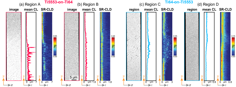
Figure 4: Description of non-uniform two-phase microstructures of additively manufactured dissimilar titanium alloys by SR-CLD and spatially-resolved mean chord lengths: (a) region of the Ti5553-on-Ti64 sample with a gradient in the size of $\alpha$ laths (white); (b) a region of the Ti5553-on-Ti64 sample with a relatively uniform microstructure; (c) a region of the Ti64-on-Ti5553 sample with a band of coarse $\alpha$ laths; (d) a region of the Ti64-on-Ti5553 sample with a relatively uniform microstructure. Note that $\alpha$ phase is shown in white here, which is inverse to images obtained by Kennedy et al. [30] (inverted for better presentation of results).

These subregions were selected to represent a variety of microstructure transitions that were present in the samples. The first two subregions include monotonic transitions from fine to coarse $\alpha$ laths (Figure 4(a,b)), while the other two subregions feature zones of coarse $\alpha$ laths surrounded by fine $\alpha$-lath microstructures (Figure 4(c,d)). Some of these microstructure transitions are captured by the moving average chord length: e.g., coarse zone in Figure 4(c,d). At the same time, the mean chord length curve has spurious peaks for the subregion shown in Figure 4(a), which can mislead to a conclusion of the presence of much larger $\alpha$ laths compared to the rest of the microstructure. SR-CLD maps present a richer description of these non-uniform microstructures. Serving as visual representations of the distributions rather than only the mean values, SR-CLD maps show not only most probable chord lengths for each zone but also their consistency and variance in chord lengths. The high probability of short chord lengths in the zones of fine $\alpha$ laths highlights the consistency of chords in a narrow range of lengths (Figure 4(a,b,d)). At the same time, the probability is distributed over a wide range of lengths for the zones with coarse laths (Figure 4(a,c,d)). Partially, the lack of clear SR-CLD peaks in zones with coarse $\alpha$ laths is associated with the fewer chords present in those zones. This is because the image of (approximately) constant width captures many fine laths and relatively few coarse laths. The SR-CLD maps conveniently indicate the insufficient number of chords for conclusive statistics with low probability spread over the entire range of chord lengths analyzed for these microstructure regions.

3.3 Alignment of experimental images for large microstructures

Composite images of large microstructure regions consist of multiple images of adjacent fields of view taken individually with a characterization instrument. In practice, seldom are images of the adjacent fields of view perfectly aligned. Analyses of large microstructures thus require an additional step of digital alignment followed by merging into large composite images, as was the case for the Ti images discussed in Section 3.2. Manual and semi-manual methods (e.g., [42]) are impractical for alignment of more than a few individual images. For example, methods that require any manual input would be challenging and extremely time-consuming to align and merge more than 900 images into the two composite microstructure images that were part of the Ti dataset. In this study, we found that SR-CLDs can be used for efficient, fully-automated, and effective alignment of numerous microstructure images.

We propose an SR-CLD-based method that aligns a pair of images by minimizing the difference between SR-CLDs calculated in the two images in horizontal or vertical direction in their overlapping region. We introduce scaled Euclidean distance as a quantitative metric of the difference between two SR-CLDs. For SR-CLDs, $P_{a}$ and $P_{b}$, calculated for two images $a$ and $b$ with a vertical/horizontal overlap of $K$ pixel rows/columns, our scaled Euclidean distance is expressed as:

$$d_{K}(P_{a},P_{b})=\frac{1}{K}\sqrt{\sum_{k=0}^{K}(P^{(k)}_{a}-P^{(k)}_{b})^{2}},$$ (2)

Note that, compared to the conventional Euclidean distance between two high-dimensional vectors, $d_{K}$ quantity has an additional factor of $\frac{1}{K}$, which normalizes the difference in two SR-CLDs by the amount of overlap between the two images, $K$. We introduce this factor because minimizing just the absolute value of the Euclidean distance would always favor a minimal overlap of two images, which does not necessarily correspond to the best alignment. Thus defined, scaled Euclidean distance serves as a quantitative alignment “error” between two images in a given direction. The process of alignment can be then formulated as an optimization problem that seeks the optimal overlap, $K_{\text{opt}}$, that minimizes the alignment error, $d_{K}$:

$$K_{\text{opt}}=\arg\min_{K}d_{K}(P_{a},P_{b})$$ (3)

Since the SR-CLD calculation is computationally efficient (see Section 4), $K_{\text{opt}}$ can be found by iteratively adjusting the relative position of images by single-pixel shifts. Starting with an exaggerated overlap such that $K\gg K_{opt}$, one of the images is shifted (pixel-wise) in the direction of separation (no overlap) of the two images (Figure 5(a)). The analysis of the alignment error calculated at different overlaps $K$ during iterative shifting (Figure 5(c)) provides $K_{\text{opt}}$ that minimizes $d_{K}(P_{a},P_{b})$. This procedure of minimizing the alignment error is suitable for vertical, horizontal, and combined alignment. For combined alignment in both directions, the images can be aligned first in one direction followed by alignment in the other direction.

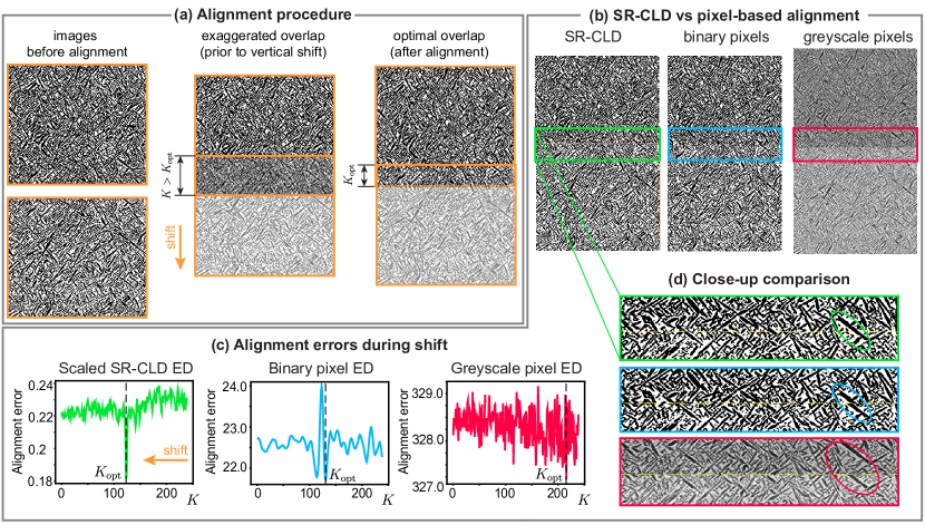
Figure 5: Alignment of images using SR-CLD. (a) Schematic showing the alignment procedure by relative shifting of images (here in vertical direction as example). Comparison of image alignment with three alignment error metrics – scaled Euclidean distance in SR-CLD; Euclidean distance in binary pixel values (0,1); and Euclidean distance in greyscale pixel values (0-255): (b) merged image following the alignment; (c) the alignment error vs. overlap (or relative shift position); (d) close-up on the “seam” region of the merged images using the three methods.

The alignment procedure described above can be used for alignment of very large series of images by repeating the steps of pairwise alignment and merging. We tested this methodology for automated alignment and merging of more than 900 images from the Ti dataset discussed above. First, the SR-CLDs were calculated for two images at a time in the vertical direction. Using these SR-CLDs, the images were aligned vertically by finding the optimal vertical overlap that minimizes the alignment error (Equation 3). Then the SR-CLDs in horizontal direction were calculated only for the overlapping rows of the two images, followed by minimizing their difference, $d_{K}$. Once two images were aligned in both directions, they were merged into a single image. The procedure was repeated for the pairwise alignment of the merged image with a next individual image. We compared this SR-CLD approach with alignment by minimizing the Euclidean distance between pixel values previously considered in literature [43, 44]. We found that the SR-CLD approach leads to better alignment (Figure 5(b,d)) because the experimental images had significant differences in image contrast, which results in noise in pixel values in the overlapped regions, whether raw or after processing and segmentation (Figure 5(b–d)). Since SR-CLDs are statistical descriptions, they are less sensitive to raw image imperfections, differences in contrast due to surface lightning, and noise or errors in segmentation [45], which results in more robust alignment (Figure 5(d)).

4 Discussion

In this work, we introduced a new approach to analyzing and quantifying non-uniform microstructures. With two case studies, we demonstrated that SR-CLDs provide insights into spatial microstructure variations inaccessible with traditional methods of microstructure descriptions. For example, two clearly different polycrystalline microstructures studied in Section 3.1 had similar overall grain size distributions and mean grain sizes (Figure 3(a,d)). SR-CLD captured the differences in those microstructure both numerically and visually via SR-CLD maps (Figure 3(b)). Capturing spatial differences is important because microstructure description is a foundation for establishing process–microstructure–property relationships. We can expect that a microstructure with a significant gradient is a result of a particular process and will have properties different from those of a uniform microstructure. Yet, microstructure descriptions that focus on overall size distributions or mean values without spatial sensitivity will fail to reflect such differences. The SR-CLD approach that resolves spatial microstructure variations can therefore serve as a statistically rigorous microstructure description for quantitative process–microstructure–property relationships in materials with significantly non-uniform microstructures. For example, SR-CLDs or their reduced-order representations (e.g., from principal component analysis [18]) could be used as microstructure “features” for machine learning, as previously shown with traditional (non-spatially-resolved) CLDs [46, 47, 21].

While our case studies demonstrated SR-CLDs for describing grains and phases, the presented approach is flexible for analyzing any other microstructure constituents in a wide variety of materials and data modalities. Since our chord length calculation is based on simple pixel counting, any microstructure map that contains constituent labels at pixels could be used for SR-CLD calculations. This includes electron back-scattered diffraction (EBSD) maps that contain phase IDs (for multiphase microstructures) and grain IDs at each EBSD “pixel”, which can be used for digital chord measurements for the SR-CLD approach. Segmented microstructure images are another wide class of microstructure data that can benefit from the presented SR-CLD calculations. An advantage of leveraging SR-CLDs for segmented images is that, CLDs are tolerant to segmentation errors inevitable in experimentally obtained microstructures [45].

In addition to the description of non-uniform microstructures, we demonstrated the application of SR-CLD for image alignment (Figure 5). Using Euclidean distance between SR-CLD in the overlapped regions of image pairs, we successfully aligned and merged over 900 images into two large composite images. Similar to the microstructure description, this SR-CLD-based alignment is robust even in the presence of contrast and segmentation differences in the images (Figure 5(d)). Like microstructure description, alignment based on SR-CLD can be used for a rich variety of microstructures, microstructure constituents, and data modalities, not limited to images of phases from the scanning electron microscope considered in Section 3.2.

Based on simple pixel counting, the presented approach of SR-CLD calculations is computationally efficient with minimum CPU and memory requirements. Calculation of SR-CLD for a typical high-resolution $12000\times 4000$ image (shown in Figure 4) takes only about $23\text{\,}\mathrm{s}$, and $6.3\text{\,}\mathrm{min}$ for a very large ($288688\times 3897$) composite image on an average consumer-grade laptop (MacBook Air M1 with $16\text{\,}\mathrm{GB}$ RAM). Since the calculation of individual location-specific CLD for a pixel row/column is independent, the SR-CLD calculation can be easily parallelized if needed, e.g., for extremely large microstructure maps. To facilitate adoption of the approach by the community, we made a Python code for SR-CLD calculations available on GitHub (link below).

5 Conclusion

In this paper, we presented calculation of spatially-resolved chord length distribution (SR-CLD) for statistical description of non-uniform microstructures. With two case studies, we demonstrated the application of our SR-CLD approach to different microstructures with grains and phases as microstructure constituents of interest. The results show that SR-CLDs capture spatial variations of constituent sizes that would be inaccessible with traditional microstructure descriptions focusing on overall size distributions or their moments. SR-CLD captures microstructure uniformity (or lack thereof) both visually (via proposed SR-CLD maps) and numerically and are therefore suitable both for intuitive visual assessment of the microstructure and for quantitative relationships between microstructure, properties, and processing. We further demonstrated that SR-CLDs can be used for robust alignment of numerous microstructure images into large composite images even in the presence of contrast and other differences in images that need to be aligned. With a simple pixel counting algorithm as a basis, SR-CLD calculations require very modest computational resources and can be therefore calculated for description or alignment of very large images on a typical laptop.

Data availability

The codes for SR-CLD calculations and SR-CLD-based alignment are available at https://github.com/materials-informatics-az/SR-CLD.

References

- [1] S. R. Kalidindi, Hierarchical materials informatics: novel analytics for materials data, Elsevier, 2015.
- [2] D. T. Fullwood, S. R. Niezgoda, B. L. Adams, S. R. Kalidindi, Microstructure sensitive design for performance optimization, Progress in Materials Science 55 (6) (2010) 477–562.
- [3] L. S. Toth, S. Biswas, C. Gu, B. Beausir, Notes on representing grain size distributions obtained by electron backscatter diffraction, Materials Characterization 84 (2013) 67–71. doi:10.1016/j.matchar.2013.07.013.
- [4] A. T. Polonsky, M. P. Echlin, W. C. Lenthe, R. R. Dehoff, M. M. Kirka, T. M. Pollock, Defects and 3d structural inhomogeneity in electron beam additively manufactured inconel 718, Materials Characterization 143 (2018) 171–181.
- [5] E. Hall, Variation of hardness of metals with grain size, Nature 173 (4411) (1954) 948–949.
- [6] N. Petch, Xvi. the ductile fracture of polycrystalline -iron, Philosophical Magazine 1 (2) (1956) 186–190.
- [7] D. M. Saylor, J. Fridy, B. S. El-Dasher, K.-Y. Jung, A. D. Rollett, Statistically representative three-dimensional microstructures based on orthogonal observation sections, Metallurgical and Materials Transactions A 35 (7) (2004) 1969–1979. doi:10.1007/s11661-004-0146-0.
- [8] A. J. Schwartz, M. Kumar, B. L. Adams, D. P. Field (Eds.), Electron backscatter diffraction in materials science, Springer, Boston, MA, 2009. arXiv:arXiv:1011.1669v3, doi:10.1007/978-0-387-88136-2.
- [9] P. Hovington, P. Pinard, M. Lagacé, L. Rodrigue, R. Gauvin, M. Trudeau, Towards a more comprehensive microstructural analysis of zr–2.5nb pressure tubing using image analysis and electron backscattered diffraction (ebsd), Journal of Nuclear Materials 393 (1) (2009) 162 – 174. doi:10.1016/j.jnucmat.2009.05.017.
- [10] S. Torquato, B. Lu, Chord-length distribution function for two-phase random media, Physical Review E 47 (4) (1993) 2950–2953. doi:10.1103/PhysRevE.47.2950.
- [11] A. P. Roberts, S. Torquato, Chord-distribution functions of three-dimensional random media: Approximate first-passage times of Gaussian processes, Physical Review E - Statistical Physics, Plasmas, Fluids, and Related Interdisciplinary Topics 59 (5) (1999) 4953–4963. doi:10.1103/PhysRevE.59.4953.
- [12] B. L. Adams, S. R. Kalidindi, D. T. Fullwood, Microstructure Sensitive Design for Performance Optimization, Elsevier Science, 2012.
- [13] B. S. Fromm, B. L. Adams, S. Ahmadi, M. Knezevic, Grain size and orientation distributions: Application to yielding of -titanium, Acta Materialia 57 (8) (2009) 2339–2348. doi:10.1016/j.actamat.2008.12.037.
- [14] S. Sun, V. Sundararaghavan, A probabilistic crystal plasticity model for modeling grain shape effects based on slip geometry, Acta Materialia 60 (13-14) (2012) 5233–5244. doi:10.1016/j.actamat.2012.05.039.
- [15] ASTM Standard, E112-13, Standard Test Methods for Determining Average Grain Size, ASTM International, West Conshohocken, PA, 2013. doi:10.1520/E0112.
- [16] P. Lehto, H. Remes, T. Saukkonen, H. Hänninen, J. Romanoff, Influence of grain size distribution on the Hall-Petch relationship of welded structural steel, Materials Science and Engineering A 592 (2014) 28–39. doi:10.1016/j.msea.2013.10.094.
- [17] P. Lehto, J. Romanoff, H. Remes, T. Sarikka, Characterisation of local grain size variation of welded structural steel, Welding in the World 60 (2016) 673–688. doi:10.1007/s40194-016-0318-8.
- [18] M. I. Latypov, M. Kühbach, I. J. Beyerlein, J.-C. Stinville, L. S. Toth, T. M. Pollock, S. R. Kalidindi, Application of chord length distributions and principal component analysis for quantification and representation of diverse polycrystalline microstructures, Materials Characterization 145 (2018) 671–685.
- [19] D. M. Turner, S. R. Niezgoda, S. R. Kalidindi, Efficient computation of the angularly resolved chord length distributions and lineal path functions in large microstructure datasets, Modelling and Simulation in Materials Science and Engineering 24 (7) (2016) 75002. doi:10.1088/0965-0393/24/7/075002.
- [20] P. Fernandez-Zelaia, O. D. Acevedo, M. M. Kirka, D. Leonard, S. Yoder, Y. Lee, Creep Behavior of a High- Ni-Based Superalloy Fabricated via Electron Beam Melting, Metallurgical and Materials Transactions A 52 (2021) 574–590.
- [21] Y. Fan, X. Yang, D. Shi, L. Tan, W. Huang, Quantitative mapping of service process-microstructural degradation-property deterioration for a ni-based superalloy based on chord length distribution imaging process, Materials & Design 203 (2021) 109561.
- [22] Y. Zhu, X. Wu, Heterostructured materials, Progress in Materials Science 131 (2023) 101019.
- [23] Y. Estrin, Y. Beygelzimer, R. Kulagin, P. Gumbsch, P. Fratzl, Y. Zhu, H. Hahn, Architecturing materials at mesoscale: some current trends, Materials Research Letters 9 (10) (2021) 399–421.
- [24] Y. Wei, Y. Li, L. Zhu, Y. Liu, X. Lei, G. Wang, Y. Wu, Z. Mi, J. Liu, H. Wang, et al., Evading the strength–ductility trade-off dilemma in steel through gradient hierarchical nanotwins, Nature communications 5 (1) (2014) 3580.
- [25] Y. Beygelzimer, R. Kulagin, P. Fratzl, Y. Estrin, The earth’s lithosphere inspires materials design, Advanced Materials 33 (3) (2021) 2005473.
- [26] A. Heidarzadeh, S. Mironov, R. Kaibyshev, G. Çam, A. Simar, A. Gerlich, F. Khodabakhshi, A. Mostafaei, D. P. Field, J. D. Robson, et al., Friction stir welding/processing of metals and alloys: A comprehensive review on microstructural evolution, Progress in Materials Science 117 (2021) 100752.
- [27] Z. Hu, Z. Ma, L. Yu, Y. Liu, Functionally graded materials with grain-size gradients and heterogeneous microstructures achieved by additive manufacturing, Scripta Materialia 226 (2023) 115197.
- [28] J. Y. Kang, J. G. Kim, H. W. Park, H. S. Kim, Multiscale architectured materials with composition and grain size gradients manufactured using high-pressure torsion, Scientific reports 6 (1) (2016) 26590.
- [29] W. C. Lenthe, J.-C. Stinville, M. P. Echlin, T. M. Pollock, Statistical Assessment of Fatigue-Initiating Microstructural Features in a Polycrystalline Disk Alloy, Superalloys 2016: 13th International Symposium (2016). doi:10.1002/9781119075646.ch61.
- [30] J. Kennedy, A. Davis, A. Caballero, M. White, J. Fellowes, E. Pickering, P. Prangnell, Microstructure transition gradients in titanium dissimilar alloy (ti-5al-5v-5mo-3cr/ti-6al-4v) tailored wire-arc additively manufactured components, Materials Characterization 182 (2021) 111577.
- [31] D. M. Turner, S. R. Niezgoda, S. R. Kalidindi, Efficient computation of the angularly resolved chord length distributions and lineal path functions in large microstructure datasets, Modelling and Simulation in Materials Science and Engineering 24 (7) (2016) 075002.
- [32] H. A. Sturges, The choice of a class interval, Journal of the american statistical association 21 (153) (1926) 65–66.
- [33] D. W. Scott, On optimal and data-based histograms, Biometrika 66 (3) (1979) 605–610.
- [34] D. Freedman, P. Diaconis, On the histogram as a density estimator: L 2 theory, Zeitschrift für Wahrscheinlichkeitstheorie und verwandte Gebiete 57 (4) (1981) 453–476.
- [35] G. R. Terrell, D. W. Scott, Oversmoothed nonparametric density estimates, Journal of the American Statistical Association 80 (389) (1985) 209–214.
- [36] D. P. Doane, Aesthetic frequency classifications, The American Statistician 30 (4) (1976) 181–183.
- [37] R. Quey, P. Dawson, F. Barbe, Large-scale 3d random polycrystals for the finite element method: Generation, meshing and remeshing, Computer Methods in Applied Mechanics and Engineering 200 (17-20) (2011) 1729–1745.
- [38] R. Quey, L. Renversade, Optimal polyhedral description of 3d polycrystals: Method and application to statistical and synchrotron x-ray diffraction data, Computer Methods in Applied Mechanics and Engineering 330 (2018) 308–333.
- [39] J.-C. Yen, F.-J. Chang, S. Chang, A new criterion for automatic multilevel thresholding, IEEE Transactions on Image Processing 4 (3) (1995) 370–378. doi:10.1109/83.366472.
- [40] L. Vincent, Grayscale area openings and closings, their efficient implementation and applications, in: First Workshop on Mathematical Morphology and its Applications to Signal Processing, Citeseer, 1993, pp. 22–27.
- [41] G. Priya, K. Nawaz, Effective morphological image processing techniques and image reconstruction, IJTRD, vol. abs/1703.10593 (2017).
- [42] J. Garnett, Misalign: A metallography image software for alignment., https://github.com/jess-garnett/MISalign (2023).
- [43] D. Kozinska, J. Tretiak, J. Nissanov, C. Ozturk, Multidimensional alignment using the euclidean distance transform, Graphical models and image processing 59 (6) (1997) 373–387.
- [44] L. Wang, Y. Zhang, J. Feng, On the euclidean distance of images, IEEE transactions on pattern analysis and machine intelligence 27 (8) (2005) 1334–1339.
- [45] S. E. Whitman, G. Hu, H. C. Taylor, R. B. Wicker, M. I. Latypov, Automated segmentation and chord length distribution of melt pools in complex 3d printed metal artifacts, Integrating Materials and Manufacturing Innovation (2023) 1–15.
-
[46]
E. Popova, T. M. Rodgers, X. Gong, A. Cecen, J. D. Madison, S. R. Kalidindi,
Process-Structure
Linkages Using a Data Science Approach: Application to Simulated Additive
Manufacturing Data, Integrating Materials and Manufacturing Innovation
6 (1) (2017) 54–68.
doi:10.1007/s40192-017-0088-1.
URL http://link.springer.com/10.1007/s40192-017-0088-1 - [47] M. Ackermann, C. Haase, Machine learning-based identification of interpretable process-structure linkages in metal additive manufacturing, Additive Manufacturing 71 (2023) 103585.