Hardware-Assisted Parameterized Circuit Execution

Abstract

Standard compilers for quantum circuits decompose arbitrary single-qubit gates into a sequence of physical $X_{\pi/2}$ pulses and virtual-$Z$ phase gates. Consequently, many circuit classes implement different logic operations but have an equivalent structure of physical pulses that only differ by changes in virtual phases. When many structurally-equivalent circuits need to be measured, generating sequences for each circuit is unnecessary and cumbersome, since compiling and loading sequences onto classical control hardware is a primary bottleneck in quantum circuit execution. In this work, we develop a hardware-assisted protocol for executing parameterized circuits on our FPGA-based control hardware, QubiC. This protocol relies on a hardware-software co-design technique in which software identifies structural equivalency in circuits and “peels” off the relevant parameterized angles to reduce the overall waveform compilation time. The hardware architecture then performs real-time “stitching” of the parameters in the circuit to measure circuits that implement a different overall logical operation. This work demonstrates significant speed ups in the total execution time for several different classes of quantum circuits.

I Introduction

A quantum processing unit (QPU) is defined by its topology (i.e., qubit-to-qubit connectivity) and its native gate set. A gate set consists of a set of native state preparations (usually chosen to be $\ket{0}$ for all qubits), a set of native single-qubit gates for all qubits, a set of native two-qubit gates between all qubit pairs, and a set of native positive operator-valued measures (POVMs; native measurements are usually chosen to be in the computational basis). Quantum compilers decompose all quantum circuits (using a set of ordered instructions) according to the QPU’s topology and gate set. Most quantum circuits are designed with a restricted set of multi-qubit gates (e.g., using only CX or CZ gates). However, generally single-qubit gates in a circuit are allowed to be arbitrary. In order to implement arbitrary rotations in $\mathsf{SU(2)}$, quantum compilers typically decompose single-qubit gates in terms of discrete physical $X_{\pi/2}$ pulses (implemented via resonant Rabi-driven pulses) and arbitrary virtual-$Z$ phase gates McKay et al. (2017), which are performed in software as a change the phase of the subsequent physical pulse. Thus, arbitrary single-qubit gates are often termed $U_{3}$ gates, as they are decomposed as unitaries that are parameterized by three distinct phases:

$$U_{3}(\phi,\theta,\lambda)=Z_{\phi-\pi/2}X_{\pi/2}Z_{\pi-\theta}X_{\pi/2}Z_{\lambda-\pi/2}\leavevmode\nobreak\ .$$ (1)

This $ZXZXZ$-decomposition reduces the time needed to implement arbitrary single-qubit gates (only a single $X_{\pi/2}$ needs to be calibrated per qubit), but comes at the cost of requiring two physical pulses per single-qubit gate (for most gates). Importantly, in this manner, all single-qubit gates are parameterized by three phases, such that implementing different single-qubit gates equates to changing the phases of the physical pulses, without needing to change any of the physical parameters of the $X_{\pi/2}$ pulses themselves (e.g., amplitude, frequency, pulse envelope, etc.).

Many classes of quantum circuits are designed to be structurally-equivalent — i.e., they contain the same structure of physical pulses, but the virtual phases in the single-qubit gates might differ. In some cases, structurally-equivalent circuits implement a different overall logic operation, as is the case for many variational quantum algorithms Cerezo et al. (2021), such as the variational quantum eigensolver Peruzzo et al. (2014), the quantum approximate optimization algorithm Farhi et al. (2014), and the circuits used for quantum machine learning Biamonte et al. (2017); Benedetti et al. (2019). On the other hand, some structurally-equivalent circuits are instead designed to be logically-equivalent, as is the case for noise tailoring methods such as randomized compiling (RC) Wallman and Emerson (2016); Hashim et al. (2021), Pauli frame randomization Knill (2004); Kern et al. (2005); Ware et al. (2021), and equivalent circuit averaging Hashim et al. (2022). Similarly, many circuits used for quantum characterization, verification, validation (QCVV) are by design structurally-equivalent (for a given circuit depth). For example, state tomography, quantum process tomography Chuang and Nielsen (1997), gate set tomography (GST) Blume-Kohout et al. (2013, 2017), randomized benchmarking (RB) Emerson et al. (2005), cycle benchmarking (CB) Erhard et al. (2019), and many others.

All of the aforementioned protocols require generating, compiling, and measuring a large ($\sim$100 – 10000) number of circuits. The naive strategy for doing so is to compile and measure sequences for each circuit independently, creating a large bottleneck on the classical side of the control hardware. However, in many cases, this is both unnecessary and time-consuming, since the waveform for structurally-equivalent circuits has already been loaded onto the hardware. In this work, we introduce a co-designed hardware-software technique that addresses the classical-bound bottlenecks for parameterized circuit execution. The technique involves two protocols — Read-Identify-Peel (RIP) and Stitch with Deft scheduling — which universally applies to any set of structurally-equivalent quantum circuits to improve their execution efficiency. Our approach identifies circuits with equivalent pulse structures, selectively compiles unique circuits (one from each batch of structurally-equivalent circuits), peels and stores the variable parameters for each circuit, and re-attaches at run time while executing on the control system. This technique reduces the compilation time by a constant factor and adds minimal runtime overhead on resource-constrained control systems. We demonstrate significant temporal gains for the overall run time for several commonly-used protocols, including RC, RB, CB, and GST.

II Parameterized Circuit Execution

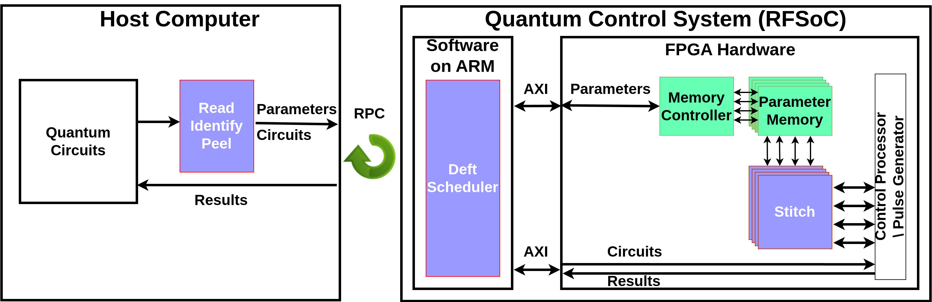
Figure 1: Block Diagram showing different parts of hardware-assisted parameterized circuit execution (PCE) with read-identify-peel (RIP) software on the host computer, deft scheduler on the control software, and stitch logic on the FPGA. The RIP on host computer separates the circuits from its parameters and compiles unique circuits and transfers them to the control system.The deft scheduler running as a software on control system schedules circuits and the appropriate parameters. The parameters and circuits are stitched back together in control system FPGA in real time. At the end of circuit execution, the results are transferred back to the host computer.

In this work, we design a hardware-assisted parameterized circuit execution (PCE) protocol by introducing two techniques — Read-Identify-Peel (RIP) and Stitch with Deft Scheduling — to improve the execution efficiency for classes of structurally-equivalent circuits. As shown in Fig. 1, the process is a hardware-software co-designed protocol involving a general purpose computer, referred to as Host Computer, an embedded software computer, referred to as Software on ARM, and a hardware design on the FPGA that runs on the control system. The software, done in Python, identifies structurally-equivalent circuits, separates the phase parameters in single-qubit gates, and orchestrates the circuit execution; the hardware performs the parameterized execution in real time. The control system in this work uses AMD (formerly Xilinx) Zynq UltraScale+ RFSoC ZCU216 evaluation kit Xilinx (2024), consisting of ARM processors and an FPGA. The deft scheduler runs on the ARM processor, and the Stitch design, written in Verilog/System Verilog, is implemented on the FPGA. The design integrates with the QubiC 2.0 control system Xu et al. (2023), an open-source FPGA-based quantum control system developed at Lawrence Berkeley National Laboratory.

II.1 Read-Identify-Peel (RIP)

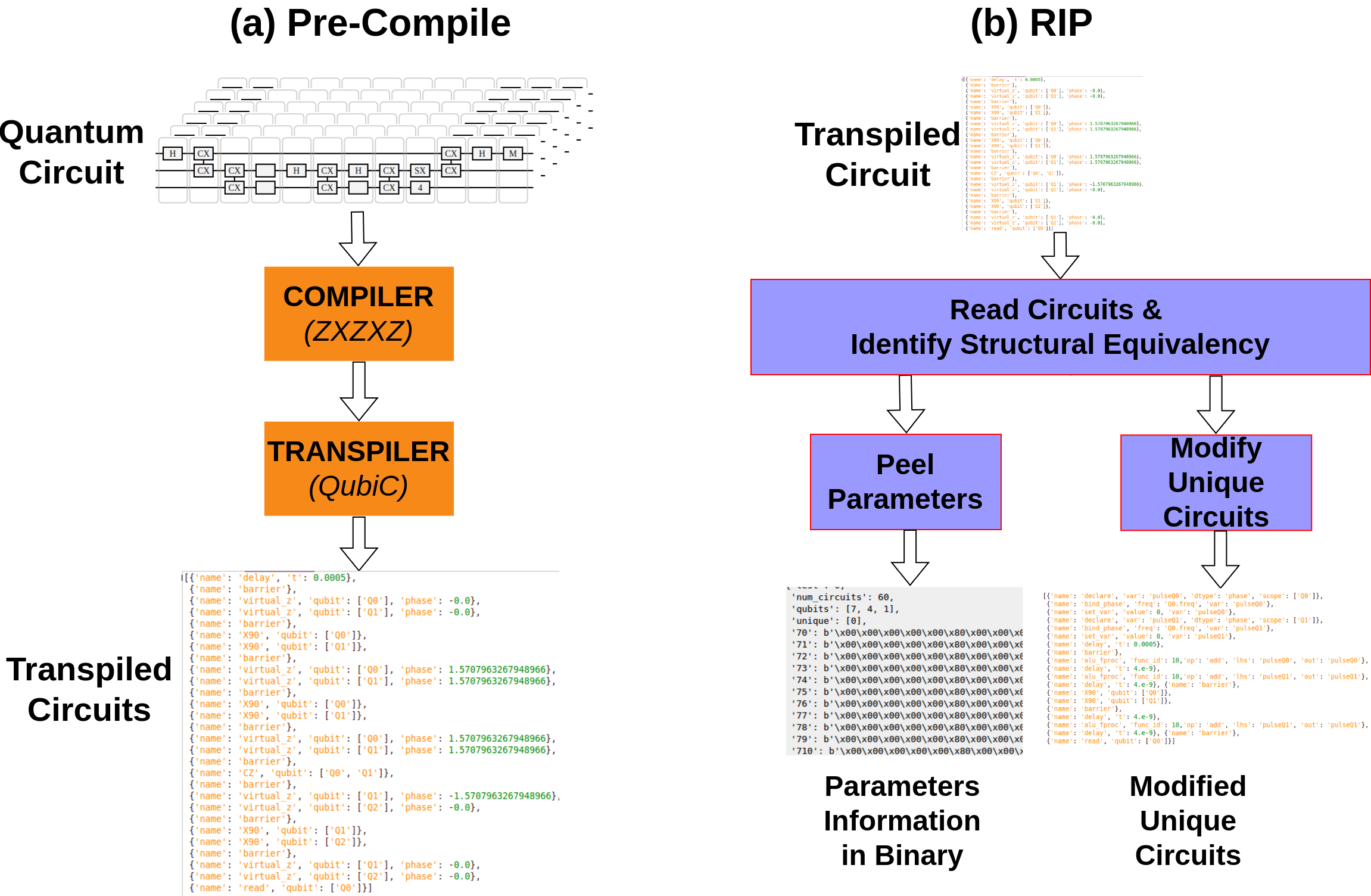
Figure 2: The read-identify-peel (RIP) process. (a) The transformation steps of a quantum circuit through compilation and transpilation. These step converts a quantum circuit written in openQASM3, Qiskit, True-Q, or pyGSTi into a QubiC circuits. (b) The parameterization steps of identifying structural equivalency in a batch of QubiC transpiled circuits, peeling the phase information from the circuits, and modifying the unique circuits (one from each structurally-equivalent batch) to request the peel phases in real-time on the FPGA.

RIP is a software process written in Python and runs on a general-purpose computer (i.e., Host Computer). Figure 2 shows the process that prepares the circuits for parameterized execution and provides the necessary information to the control system’s deft scheduler and the Stitch process. The RIP technique is generic and can be adapted (with minimal changes) to any circuit abstraction. Currently, the process integrates to the native control system gate format, QubiC, and has been tested with circuits written/compiled in openQASM3 Cross et al. (2022), Qiskit Javadi-Abhari et al. (2024), True-Q Beale et al. (2020), pyGSTi Nielsen et al. (2019), and QubiC-native gate abstraction. As shown in Fig. 2a, the circuit abstraction-specific compiler (e.g., a compiler for openQASM3, Qiskit, True-Q, or pyGSTi circuits) compiles the circuit into native single- and two-qubit gates, where the single-qubit gates are decomposed according to Eq. 1. The QubiC transpiler converts these compiled circuits into QubiC instructions, which is the input to the RIP stage.

The Read-Identify method identifies the structural equivalency in a batch of circuits. The process reads each circuit in the list of circuits and creates a set of graphs for each circuit. Each graph consists of a root node for the target qubits and the gates associated with it in the same timing order. After constructing the graph for a circuit, the process compares the graph for structural equivalency in the previous circuit graph. If the graph does not match any prior graph, the circuit is unique. Each unique circuit is added as a new sublist in the list of circuit indices and marked for circuit modification. If there is equivalency, then the circuit index is appended to the sublist of the equivalent circuit index. After reading all the circuits in the batch, the process identifies structurally-equivalent circuits as a list of circuit indices, where each sublist has all the structurally-equivalent circuits and the first index depicting the unique circuit. The flattened list of lists will provide the circuit execution order for the deft scheduler. The computational complexity of finding equivalency is $\mathcal{O}(n^{2})$, where $n$ is the number of circuits. Depending on the algorithm, similar circuits can be next to each other (for RC, RB, and CB circuits) or in a random order in the batch (in the case of GST). The read-identify process can automatically identify the structural equivalency in both scenarios.

The Peel method extracts the parameters from the circuits. The process uses the graph from the Read-Identify process to extract the parameters from each of the circuits. The extraction identifies the graph nodes with desired parameters (e.g., virtual-$Z$ phases) and creates a dictionary based on the circuit and the target physical qubit. The entire dictionary is then binarized and transmitted to the deft scheduler. The binarization is a performance method and provides up to $15\times$ speed up compared to transmitting a non-binarized dictionary.

Modification of circuits is the final method in the RIP process. The unique circuits marked during the Read-Identify phase are modified to request the phase in real time. This process replaces the parameter instructions (virtual-z), from where the peel method has extracted the phases, into a phase request instruction, alu_fproc. These instructions are specific to the QubiC distributed processor and request the phase from the Stitch module in FPGA. In QubiC terms, the Stitch module acts as a Function Processor Fruitwala et al. (2024a), or fproc.

II.2 Stitch

The Stitch process re-attaches the parameters from the RIP process in the FPGA. The Stitch module consists of three subcomponents: the memory controller, parameter memory, and the stitch logic. The memory controller interfaces with the ARM processor for the read/write of the parameters, the parameter memory holds the parameter values, and the stitch logic interacts with the QubiC distributed processor for parameterized circuit execution. The Stitch modules are highly modularized and extensible for several qubits. The current design is written in a combination of Verilog and System Verilog, and runs at the clock speed of 500 MHz, supporting parameterization of up to eight physical qubits.

The QubiC control system uses the Zynq UltraScale+ RF-SoC ZCU216 evaluation kit as the hardware platform. The development board consists of ARM processors and FPGA running in different frequency domains. The ARM processor runs up to $1.33$ GHz and connects to the extensible parameter memory on FPGA running at $500$ MHz (design choice) via an AXI bus running at $100$ MHz (the Full Power Domain bus). The memory controller is a cross-clock domain module interacting with the single AXI bus and the parallel parameter memory interface. Within the controller lies a single-stage switch that translates the AXI memory map to the parameter memory map. The current mapping is a 32-bit AXI to a 14-bit parameter memory; of the 14-bit, the first 3 bits map the eight parallel memories of $2^{11}$ bytes.

The parameter memory is an FPGA Block RAM (BRAM) containing parallel memories for each physical qubit (eight memories in the current implementation). Each parallel memory is 8 kilobytes and holds up to 2048 32-bit parameters per circuit. Each memory is a true dual-port (TDP) design, with one interface to the controller and the other to the stitch logic. In a normal parameterized circuit execution, the memory controller interface writes the parameter to the memory, and the stitch logic reads from the memory. The rest of the read and write bus, i.e., read from memory controller and write from stitch logic, are only used for debugging.

The stitch logic block is the heart of the hardware-assisted parameterization and interacts with the parameter memories and the QubiC control system’s distributed processor. The current design hosts eight parallel interfaces for the memory and eight fproc interfaces for the processor. The fproc interface requests the parameters, and the stitch logic pulls them from the parameter memory and provides them back to the fproc. Since the request pulls are sequential, the logic uses prefetch functionality to improve performance and completes a parameter request within 4 ns. Further, each quantum circuit typically runs for N times (shots), and the stitch logic tracks the number of parameters in a circuit and repeats itself for N times. Also, the architecture supports the existing mid-circuit measurement functionality. The request type between a parameter and a mid-circuit measurement from the control processor is distinguished using the core_id parameter in the fproc interface. Additionally, the logic can repeat a partial set of the parameters and switch to a different set. The control codes set by the deft scheduler before circuit execution facilitate these functionalities.

II.3 Deft Scheduler

Deft Scheduling orchestrates the circuit execution by interacting with the RIP and the Stitch layer. The scheduler is Python software running on the ARM processor on the control hardware. It integrates with the existing QubiC software API infrastructure by adding methods to the CircuitRunner class. The integration allows users to use the PCE functionality with the existing QubiC API infrastructure. On the control side, the scheduler creates new methods (low-level memory drivers) for circuit and parameter loading. It reuses the QubiC load definitions for writing the envelope and frequency parameters, run-circuit to trigger the circuit run, and get-data methods for collecting the data.

The deft scheduler receives a dictionary of parameters and the modified unique circuits from the host computer via a remote procedure call (RPC). The scheduler de-binarizes the parameter dictionary to read the circuit order and parameters. It takes the index from the circuit order and loads the parameters to the parameter memory in the FPGA. It loads the circuit only if the index belongs to the unique circuit list. Once the parameters and circuits are loaded, the scheduler continues the standard software operations by loading the definitions (controlled by user flags), running the circuits, receiving the data from the FPGA, and transferring data to the host computer.

III Time Profiling

The PCE protocol should reduce the execution time of quantum circuits. As seen in Sec. II, a quantum circuit execution consists of multiple steps over different computational domains, such as the host computer and the control system. Understanding the efficacy of PCE requires detailed time profiling of each step in the execution process. Thus, we added a time profiling infrastructure to QubiC to measure the time at different stages.

III.1 Time Profiling Infrastructure

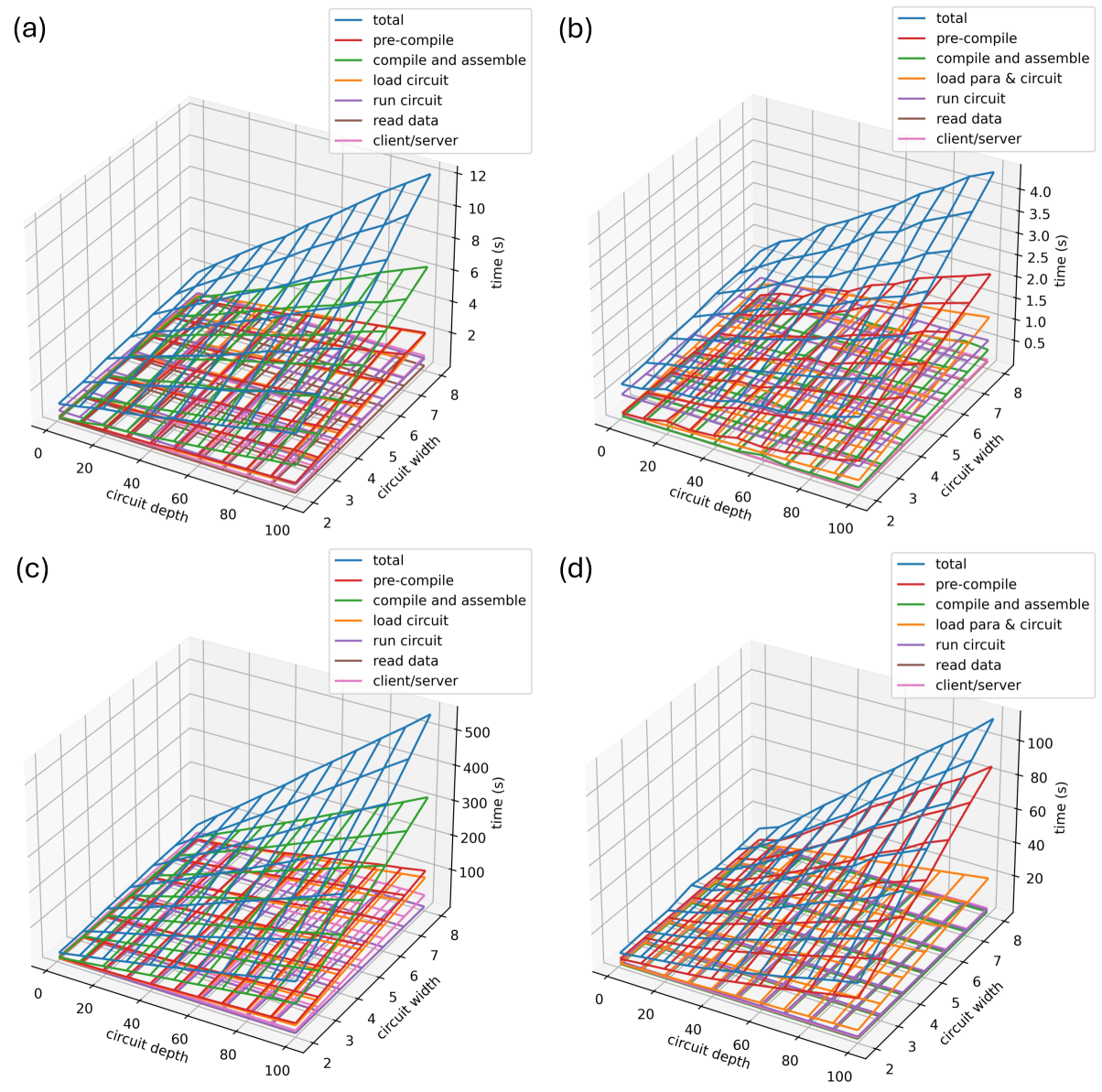
Figure 3: Time Profiling. We compare a breakdown of the execution time for performing RC on circuits of various widths (2- 8 qubits) and depths (1 – 100 cycles of two-qubit gates) using the software-based and parameterized RC protocols. For the software protocol, we implement RC using (a) 20 and (c) 1000 different randomizations over a total of 1000 shots. The parameterized protocol gives a $\sim 3\times$ and $\sim 5\times$ speedup over software RC for (b) $N=20$ and (d) $N=1000$ randomization, respectively.

The time profiling presented here occurs at three layers: the application, the host computer software, and the control system software. Each layer has multiple classical computation stages; in some cases, each stage has sub-stages of operations. During a circuit execution, these stages and sub-stages may run for varying iterations. For example, to run a single circuit for 100 shots, the compilation and the circuit load stage run once, whereas the run circuit stage has 100 iterations (1 per shot). The profiler captures the time spent on all the stages and sub-stages at different layers for varying iterations, and collects them into a Python dictionary. For ease of use, the profiling infrastructure integrates with the control software layer and allows the user to control the time profiling for all layers from the application layer.

Application Layer: this layer is the front end of the circuit execution. The experiments in this manuscript run as a Jupyter Notebook on an Intel i9-11900K desktop processor. Typically, this layer is responsible for circuit creation, pre-compilation, parameterization and control software initiation, and result display. The different profiling stages in this layer are as follows:

• Pre-compile creates or reads circuits, compiles, and transpiles to a native control system gate format. This stage refers to the process described in Section II.1 and Fig. 2(a). Even though this is a compilation stage, the word ‘Pre-Compile’ is chosen to differentiate the compile stage in the host computer software layer, which converts the circuits into pulse definition. The pre-compile stage has the following sub-stages:

  • Get circuit provides the circuit by generating or reading a pre-generated circuit from the file.

  • Transpile converts the circuit shown in Eq. 1 into the native control software gate format.

• RIP is the software parameterization stage identifying the structural equivalency, extracting the phases, and modifying the circuit for PCE.

• Active is an optional stage to convert a circuit from a passive reset ($500\mu s$ in current QPU) to an active reset circuit.

• Build Run transfers the control from the application layer to the host computer software layer and receives the quantum data from the control system.

• Total is the complete execution time from the start of circuit creation to the display of the result for an experiment.

Host Computer Software Layer: the application layer initiates this layer for circuit execution. Like the application layer, this layer also runs on the desktop as a Python module. This layer initiates the circuit execution by compiling and assembling the circuit and transferring the output to the software running on the control hardware by acting as a client in a remote procedure call (RPC). After the circuit execution, it reads the data from the RPC server running on the control hardware and passes it to the application layer. This layer has the following stages and sub-stages:

• Compile converts the circuit from the native control software gate format into control hardware-specific assembly instructions.

• Assemble converts the assembly language instructions into a machine code.

• RunAll on Host covers the time to run the circuits and get the result data.

  • Run on Host measures the run time of the circuits from the host computer.

  • Data Sort converts the raw IQ data into a distribution of bit strings.

• Client/Server is a post-processing calculation for measuring the time taken for data transmission between the RPC client and server.

Control Software Layer: the control software layer runs on the ARM processor of the control hardware platform (AMD ZCU216 RFSoC) as a Python module. The control software receives the circuits and the execution parameters from the host computer software layer via the RPC protocol. The control software interacts with the control hardware FPGA to load all the circuit elements, run the circuits, and collect the data. This process has the following stages:

• Load Batch transfers all the circuit parameters from the ARM processor to different memories in the FPGA. This stage has the following sub-stages:

  • Load circuit transfers the quantum circuits from the ARM processor to the command memory in FPGA.

  • Load definition is a multi-stage loading of circuit parameters such as signal envelope and frequencies.

  • Load env. transfers the signal envelope.

  • Load freq. transfers the frequency parameters.

  • Load zero clears the command buffer.

• Load para transfers the parameters peeled in RIP to the parameter memory in FPGA.

• Run Batch starts with the run trigger to start the circuit execution and ends with getting the quantum data.

  • Start Run measures the run time of the circuit on the FPGA.

  • Get data is the time to read the quantum measurement data from the FPGA.

• Stitch is a post-processing measurement for the stitch module to serve the stitch request inside FPGA.

III.2 Randomized Compiling

To benchmark the runtime improvements of PCE for classes of equivalent circuits, we profile the total execution time of random circuits at varying depths (from 1 – 100, defined by the number of two-qubit gate cycles) and widths (2 – 8 qubits) measured with randomized compiling (RC), shown in Fig. 3. We measure each circuit under RC with $N=20$ randomization (50 shots/randomization) and $N=1000$ randomization (1 shot/randomization). The latter case is called the fully randomly compiled (FRC) limit Fruitwala et al. (2024b), since each randomization is measured a single time. We generate RC circuits using True-Q Beale et al. (2020) for both the software and parameterized protocols. The software implementation follows the existing QubiC software infrastructure to generate sequences and upload them to the control hardware for each randomization. The PCE implementation follows the RIP and Stitch protocols. The experiment details for the different RC cases are listed in Appendices A.1 and A.2.

In Fig. 3(a) and (b), we plot the profiling results for the software and parameterized RC results with $N=20$ randomization, respectively. In Fig. 3(c) and (d), we plot the profiling results for the software and parameterized RC results with $N=1000$ randomization, respectively. We observe that parameterized RC provides a $\sim 3\times$ and $\sim 5\times$ speedup over software RC for $N=20$ and $N=1000$ randomizations, respectively. For software RC, the main temporal bottleneck is compile and assemble due to the need to compile many different circuits from QubiC-IR to the low-level machine code. For parameterized RC, the main temporal bottleneck is pre-compile, stemming from the compilation of circuits into the native gates.

IV Validation, Benchmarking, and Characterization

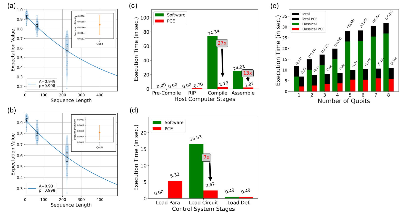
Figure 4: Randomized Benchmarking. Single-qubit RB result for (a) software RB and (b) parameterized RB. The SPAM parameter $A$ and exponential fit parameter $p$ are included in the legends for both plots. The circular data points are the results of individual circuits, and the violin plots depict the distribution of results at each circuit depth. The process of infidelity is plotted in the inset in each figure. The two results have a perfect agreement (up to the uncertainty). (c) Breakdown of the host-side time profiling for the single-qubit results in (a) and (b). PCE is $27\times$ and $13\times$ faster for the compile and assemble stages, respectively. (d) Breakdown of the control-side time profiling for the single-qubit results in (a) and (b). PCE is $7\times$ faster at the load circuit stage, but has the added cost of loading the parameters and stitching them back into the circuit. (e) Time profile of (simultaneous) RB for qubit numbers varying from $1$ to $8$. The plot represents the total execution time for the software and parameterized execution. The numbers in the parentheses show the classical time (all stages described in Section III.1 minus the StartRun stage) and the total execution time. We observe that the parameterized execution is $\sim 1.8\times$ – $3.1\times$ faster, and the improvement increased for larger numbers of qubits.

The PCE protocol applies to many classes of circuits and is primarily beneficial in the regime in which a large number of structurally-equivalent circuits need to be measured. A prototypical example of this is benchmarking and characterization circuits. For example, the circuits to perform quantum process tomography (QPT) are identical, except for a change in preparation and measurement basis. Basis rotations can be expressed in terms of combinations of a single physical gate (e.g., $X_{\pi/2}$) and virtual $Z$ gates; in this case, many QPT circuits will have the same structure of physical pulses which differ only by a change in virtual phase. Here, we validate the performance of our PCE protocol against the standard protocols for randomized benchmarking (RB) Emerson et al. (2005); Knill (2004); Magesan et al. (2011), cycle benchmarking (CB) Erhard et al. (2019), and gate set tomography (GST) Blume-Kohout et al. (2013, 2017); Nielsen et al. (2021).

IV.1 Randomized Benchmarking

A depth $m$ RB circuit consists of $m$ randomly sampled Clifford gates and a single inversion gate at the end rotates the system back to the starting state. For single-qubit RB, all single-qubit Cliffords can be decomposed into native gates and virtual phases via Eq. 1. Thus, a depth $m$ single-qubit RB circuit consists of $2(m+1)$ physical $X_{\pi/2}$ gates, and $3(m+1)$ virtual $Z$ gates. This makes RB an ideal candidate for PCE since all waveforms for a given circuit depth are structurally equivalent. In Fig. 4, we plot single-qubit RB results measured using the standard “software”-based procedure, whereby all circuits are independently sequenced and measured, and compare the results to the same circuits executed using PCE. We observe perfect agreement between the two (up to the uncertainty), with a process infidelity (i.e., error per Clifford) of $1.7(2)\times 10^{-3}$ and $1.5(1)\times 10^{-3}$ for the software and PCE results, respectively.

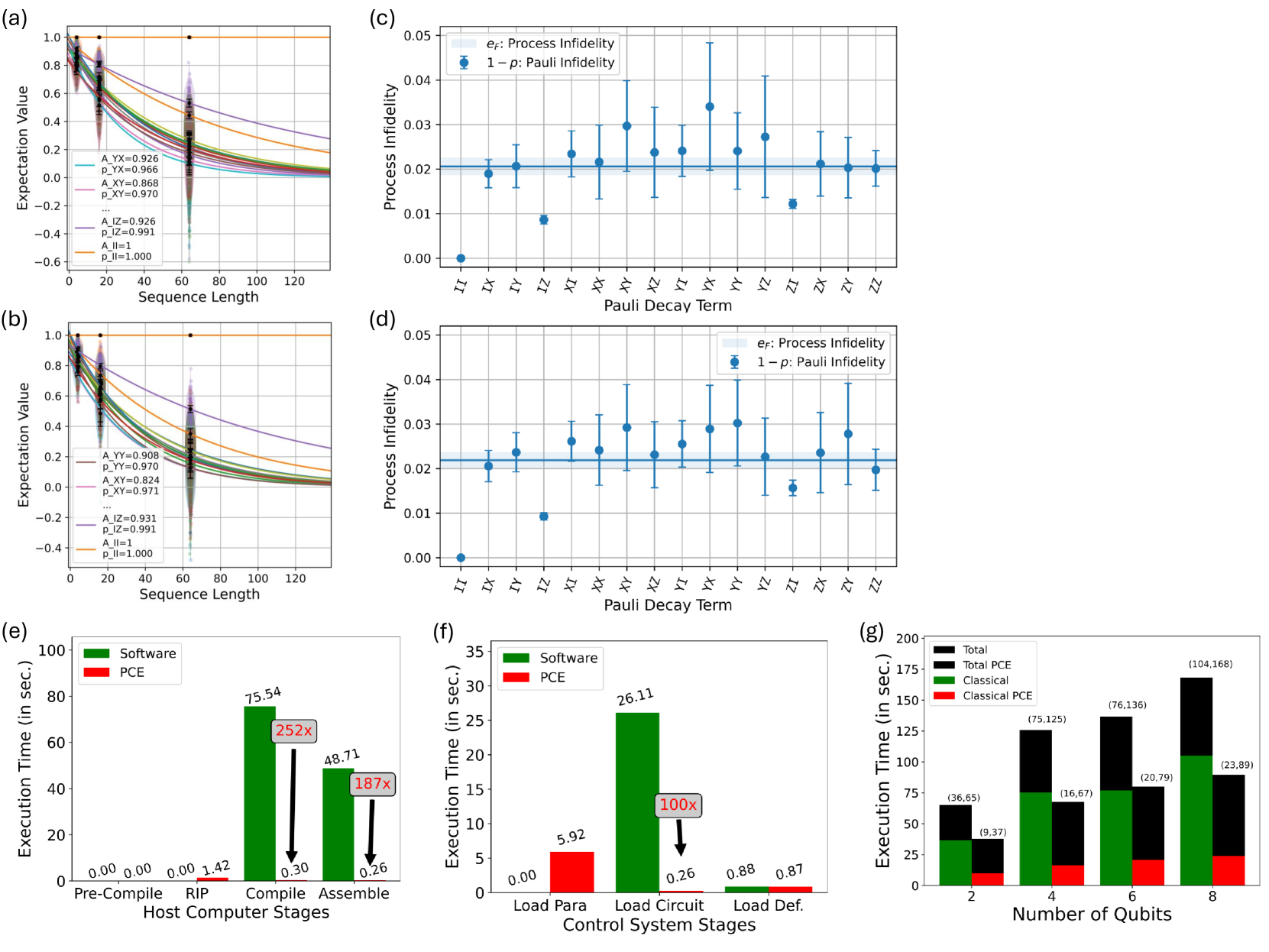
Figure 5: Cycle Benchmarking. Exponential decays for (a) software CB and (b) parameterized CB performed on a two-qubit CZ gate. Each Pauli decay is fit to an independent exponential function, with $A_{P}$ and $p_{P}$ denoting the SPAM (state-preparation and measurement) constant and the exponential fit parameter for each Pauli basis state $P$, respectively. The circular data points are the results of individual circuits, and the violin plots depict the distribution of results for each Pauli decay at each circuit depth. The Pauli infidelities and process infidelity of the gate are plotted in (c) and (d) for the results in (a) and (b), respectively. The process infidelities of both experiments are equal (up to uncertainty). (e) Breakdown of the time profiling for the results in (a) and (b). PCE is $252\times$ and $187\times$ faster for the compile and assemble stages, respectively. (f) Breakdown of the control-side time profiling for the single-qubit results in (a) and (b). PCE is $100\times$ at the load circuit stage but has the added cost of loading the parameters and stitching them back into the circuit. (g) Time profile of CB for qubit numbers varying from $2$ to $8$. The plot represents the execution time for the software and parameterized execution. The numbers in the parentheses show the classical time (all stages described in Sect. III.1 minus the StartRun stage) and the total execution time. We observe that the parameterized execution is $3.8\times$ – $4.7\times$ faster.

In Figs. 4(c) and (d), we profile the time it takes to perform RB on the host and control systems, respectively using the experiment parameters described in Appendix A.4. We observe that PCE provides a $27\times$ speedup for the compile stage and a $13\times$ speedup for the assemble stage on the host computer. On the control side, we observe a $7\times$ speedup for loading the circuits, but we have an additional cost of loading the parameters onto the FPGA. Altogether, we observe a $4\times$ speedup in the classical side of performing RB, and a $2.5\times$ speedup for the overall run time, as shown in Fig. 4(e) (here, the quantum measurement time is the same in both cases, since the total number of shots is the same). Also shown in Fig. 4(e) is a comparison of the total execution time for software-based and PCE-based RB when the number of qubits is scaled from 1 to 8. The speed up in Fig. 4(e) is lower compare to Fig. 4(c) and (d) for two reasons. First, the data read back time, which are constant for both software and PCE adds $\leavevmode\nobreak\ 22$ seconds which $10\%$ of the overall classical time as given in Table 2. Second, the circuit runtime with a passive reset of $500ns$, which adds to $23\%$ of runtime. We observe that while the classical cost of both the software and PCE protocols scales linearly in the number of qubits, this cost grows much more rapidly for the software-based protocol than for PCE, demonstrating that PCE gives us a larger relative speedup as the number of qubits grows.

It should be noted that PCE might not provide drastic improvements for all protocols. For example, for two-qubit RB, one must decompose a two-qubit Clifford gate to native gates, which does not always result in the same number of native operations (any two-qubit unitary can be expressed in as little as one native two-qubit gate or as much as three native two-qubit gates). Therefore, not all circuits at a given circuit depth will be structurally-equivalent, limiting the effectiveness of the protocol.

IV.2 Cycle Benchmarking

A depth $m$ CB circuit consists of $m$ interleaved cycles of $n$ random Pauli gates followed by an $n$-qubit gate cycle, as well as a single cycle of Paulis at the end of the sequence which rotates the system back to the Pauli eigenstate in which it started. Thus, all CB circuits of a given depth are structurally-equivalent and can be implemented with PCE, since the single-qubit Pauli gates are decomposed according to Eq. 1 and the $n$-qubit gate cycle is decomposed in a manner which depends on the gates in the cycle. Here, our interleaved gate is a two-qubit CZ gate, a native gate in our system, and is directly compiled down to the pulse definition of the gate. In Figs. 5(a) – (b), we plot the exponential decays for CB measured using the standard “software”-based procedure, whereby all circuits are independently sequenced and measured, and compare the results to the same circuits executed using PCE. In Fig. 5(c) – (d), we plot the individual Pauli infidelities (which define the different bases in which the system is prepared and measured), as well as the average process infidelity; we find that the software and PCE results are in perfect agreement (up to the uncertainty), with a (dressed) CZ process infidelity of $2.1(1)\times 10^{-2}$ and $2.19(9)\times 10^{-2}$ for the software and PCE results, respectively.

In Figs. 5(c) and (d), we profile the time it takes to perform CB on the host and control systems based on experiment parameters described in Appendix A.3. We observe that PCE provides a $252\times$ speedup for the compile stage and a $187\times$ speedup for the assemble stage on the host computer. These values are greater than for RB because CB typically requires more circuits than RB (due to the need to prepare and measure different bases). On the control side, we observe a $100\times$ speedup for loading the circuits, but we have the additional cost of loading the parameters onto the FPGA. Altogether, we observe a $5\times$ speedup in the classical side of performing CB and a $1.8\times$ speedup for the overall run time, as shown in Fig. 5(g). As mentioned in RB, the CB is also affected by the read which is $28\%$ of the overall classical time as given in Table 2, and the runtime which constitutes for $44\%$ of the total execution time. Moreover, similar to RB, the classical run time improvement gets larger as we scale the number of qubits from 2 – 8.

IV.3 Gate Set Tomography

	Standard GST	GST with PCE
Entanglement Inf. ($X_{\pi/2}$ on Q2)	0.00446	0.003901
Entanglement Inf. ($Y_{\pi/2}$ on Q2)	0.004187	0.003061
Entanglement Inf. ($X_{\pi/2}$ on Q3)	0.002952	0.003238
Entanglement Inf. ($Y_{\pi/2}$ on Q3)	0.003429	0.003991
Entanglement Inf. (CZ)	0.021482	0.020235
Model Violation ($N_{\sigma}$ @ $L=128$)	2671.78	411.152

Table 1: Comparison of GST Metrics with the standard GST run on the software and with PCE.

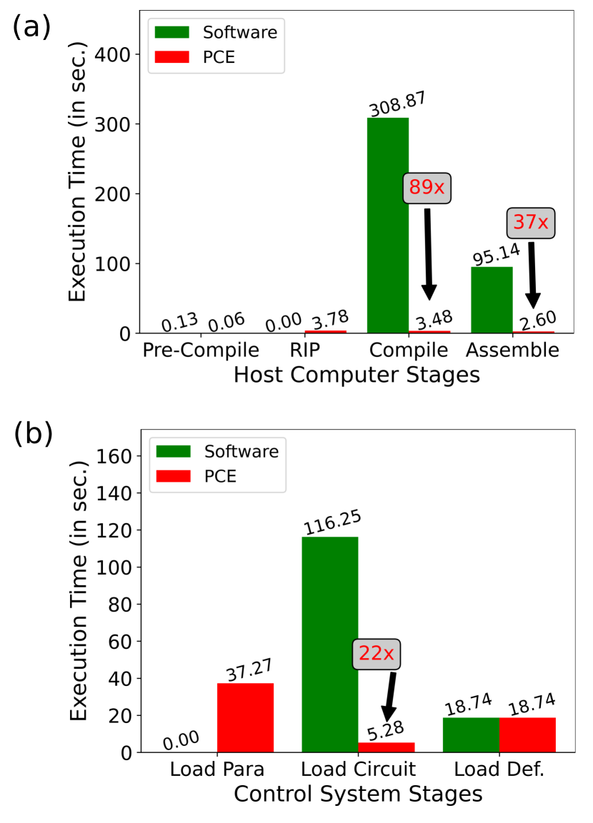
Figure 6: Gate Set Tomography. Comparison of time profiling for GST with and without PCE on the (a) host side and (b) control side. PCE is $89\times$ and $37\times$ faster for the compile and assemble stages, respectively, and $22\times$ faster at the load circuit stage.

Protocol	Number of Circuits	Structural-Equivalency (%)	Number of Unique Circuits	Classical Time(%)	Classical Time Reduction(%)	Classical Speedup ($\times$)
RC20	1540	95.00	77	94.03	64	2.55
RC FRC	77000	99.90	77	98.99	77	4.32
CB	3240	99.57	12	55.64	80	4.73
RB	736	95.65	32	76.92	78	4.37
GST	19488	98.71	251	13.34	85	6.86

Table 2: Impact of PCE with classical time speedup for various protocols. The data shows the total number of circuits, the percentage of classical time, the structurally-equivalent circuits identified by RIP, classical time reduction, and the speedup of PCE for each experiment based on the parameters described in Appendix A. The structurally-equivalency, identified by RIP, shows significant similarities with $<5\%$ of unique circuits. The classical time is the percentage of total time excluding the quantum run time with a passive reset of $500ns$. The classical time reduction shows the impact, reducing the overall classical time by $64\%$ to $85\%$ depending on the protocol. Additionally, the overall speedup considering the run time with the classical time varies between $2.55\times$ to $6.86\times$ showing a substantial reduction in quantum circuit execution.

Tomographic reconstruction methods, such as QPT and GST, scale exponentially in the number of qubits and are thus typically a very costly form of gate characterization. While PCE cannot change the poor scaling of tomography, it can improve their runtime performance, since there is a high degree of degeneracy in circuit structures, particularly for long-sequence GST. To demonstrate this, we perform two-qubit GST with and without PCE (Appendix A.5 describes the experiment parameters), and summarize some of the relevant performance metrics in Table 1. We observe that the estimated entanglement infidelities for all of the gates in the gate set (except $Y_{\pi/2}$ on Q2) are equal up to $10^{-3}$ ($10^{-2}$) for the single-qubit gates (two-qubit CZ gate). However, we observe that the model violation ($N_{\sigma}$) is significantly lower for PCE (411) than for the standard case (2672), suggesting that the GST model for the PCE data is more trustworthy. This could be, in part, due to the fact that PCE reduces the total execution time (see Table 2), and thus would be less susceptible to any kind of parameter drift during the execution of the circuits.

In Figs. 6(a) and (b), we profile the time it takes to perform GST on the host and control systems, respectively. We observe that PCE provides an $89\times$ speedup for the compile stage and a $37\times$ speedup for the assemble stage on the host computer. On the control side, we observe a $22\times$ speedup for loading the circuits, but we have the additional cost of loading the parameters onto the FPGA. Altogether, we observe a $6.86\times$ speedup in the classical side of performing GST. Even though, as shown in Table 2, the classical time for GST is about $13.34\%$.

V Conclusions

In this work, we develop a protocol for implementing parameterized circuits on our FPGA-based control hardware, QubiC. Our protocol — PCE — incorporates both software and hardware components for identifying structurally-equivalent circuits, determining the parameterized rotation phases and storing them in memory on the FPGA, and stitching these phases back into a physical waveform loaded onto the FPGA for measuring different circuits. We demonstrate significant time savings for a number of different benchmarking and characterization protocols, highlighted in Table 2. Depending on the protocol, we observe a reduction of classical time by $64\%$ to $80\%$ and a speedup of between $2.55\times$ and $6.86\times$.

PCE can be applied to many different classes of circuits, and the examples shown here are only representative of typical workflows in QCVV. However, many classes of — for example variational circuits Cerezo et al. (2021) — are parameterizable, and future work could explore other applications that could benefit from PCE. Additionally, calibrating quantum gates often requires sweeping a pulse definition over many different pulse parameters, and adapting PCE to gate calibration could lead to significant time savings in processor bring-up. Finally, we believe that PCE is an important example of how classical control hardware can be utilized to reduce the overhead in quantum workflows, and, in addition to related co-designed protocols developed for QubiC Fruitwala et al. (2024b); Vora et al. (2024), we plan to explore more ways in which classical resources can be utilized to improve the efficiency of quantum computations.

Acknowledgments

The majority of this work was supported by the Laboratory Directed Research and Development Program of Lawrence Berkeley National Laboratory under U.S. Department of Energy Contract No. DE-AC02-05CH11231. Y.X., I.S., and G.H. acknowledge financial support for the primary development of the QubiC hardware from the U.S. Department of Energy, Office of Science, Office of Advanced Scientific Computing Research Quantum Testbed Program under Contract No. DE-AC02-05CH11231 and the Quantum Testbed Pathfinder Program.

Author Contributions

A.D.R. designed the RIP and Stitch method and performed the experiments. A.D.R. and A.H. performed the data analysis. N.F., Y.X., and G.H. developed the classical control hardware QubiC used in this work. J.H. assisted in the design and analysis of the GST data. A.D.R. and A.H. wrote the manuscript with input from all coauthors. I.S., K.K., and K.N. supervised all work.

Competing Interests

The hardware-assisted parameterized circuit execution presented in this work is protected under the U.S. patent application no. 63/651,049 (patent pending), filed by Lawrence Berkeley National Laboratory on behalf of the following inventors: A.D.R., N.F., A.H., K.N., G.H., Y.X., and I.S.

Data Availability

All data are available from the corresponding author upon reasonable request.

Appendix A Experiment Parameters

Below are the experiment parameters used for profiling in Sections III and IV. Each circuit uses a delay of $500ns$ per shot to ensure starting at the ground state (passive reset).

A.1 Randomized Compiling - RC 20

• depths : [1, 10, 20, 30, 40, 50, 60, 70, 80, 90, 100]

• widths : [(0,1), (0,1,2), (0,1,2,3), (0,1,2,3,4),

• (0,1,2,3,4,5), (0,1,2,3,4,5,6), (0,1,2,3,4,5,6,7)]

• randomization per depth and width : 20

• Total number of circuits :

• randomization*depth*width $20*11*7=1540$

• shots per depth and width :

• 50 per randomization = $50\times 20=1000$

A.2 RC Fully Randomly Compiled - RC FRC

• depths : [1, 10, 20, 30, 40, 50, 60, 70, 80, 90, 100]

• widths : [(0,1), (0,1,2), (0,1,2,3), (0,1,2,3,4),

• (0,1,2,3,4,5), (0,1,2,3,4,5,6), (0,1,2,3,4,5,6,7)]

• randomization per depth and width : 1000

• Total number of circuits

• randomization*depth*width = $1000*11*7=7700$

• shots per depth and width

• 1 per randomization = $1\times 1000=1000$

A.3 Cycle Benchmarking - CB

• widths : [(0,1), (0,1,2,3), (0,1,2,3,4,5),

• (0,1,2,3,4,5,6,7)]

• randomization : [[4, 16, 64], [4, 8, 32], [2, 4, 8],

• [2, 4, 8]]

• number of circuits per width : [540, 660, 960, 1080]

• Total number of circuits : $540+640+960+1080=3240$

• shots per circuit : 100

A.4 Randomized Benchmarking - RB

• widths : [(0),(0,1), (0,1,2), (0,1,2,3), (0,1,2,3,4),

• (0,1,2,3,4,5), (0,1,2,3,4,5,6), (0,1,2,3,4,5,6,7)]

• randomization : [(16,128,384), (16,96,384),

• (16,64,256), (16,64,192), (8,64,192), (8,32,160),

• (4,32,160), (4,32,128)]

• number of circuits per width :

• (randomization * number of circuit per randomization) + read circuits = $3\times 30+2=90+2=92$

• Total number of circuits : circuit per width * width = $92*8=736$

• shots per circuit : 100

A.5 Gate Set Tomography - GST

• depths : [2, 4, 8, 16, 32, 64, 128]

• widths : [(0,1)]

• Total number of circuits : 19488

• shots per circuit : 1000

References

- McKay et al. (2017) D. C. McKay, C. J. Wood, S. Sheldon, J. M. Chow, and J. M. Gambetta, Physical Review A 96, 022330 (2017).
- Cerezo et al. (2021) M. Cerezo, A. Arrasmith, R. Babbush, S. C. Benjamin, S. Endo, K. Fujii, J. R. McClean, K. Mitarai, X. Yuan, L. Cincio, et al., Nature Reviews Physics 3, 625 (2021).
- Peruzzo et al. (2014) A. Peruzzo, J. McClean, P. Shadbolt, M.-H. Yung, X.-Q. Zhou, P. J. Love, A. Aspuru-Guzik, and J. L. O’brien, Nature communications 5, 4213 (2014).
- Farhi et al. (2014) E. Farhi, J. Goldstone, and S. Gutmann, arXiv preprint arXiv:1411.4028 (2014).
- Biamonte et al. (2017) J. Biamonte, P. Wittek, N. Pancotti, P. Rebentrost, N. Wiebe, and S. Lloyd, Nature 549, 195 (2017).
- Benedetti et al. (2019) M. Benedetti, E. Lloyd, S. Sack, and M. Fiorentini, Quantum Science and Technology 4, 043001 (2019).
- Wallman and Emerson (2016) J. J. Wallman and J. Emerson, Phys. Rev. A 94, 052325 (2016).
- Hashim et al. (2021) A. Hashim, R. K. Naik, A. Morvan, J.-L. Ville, B. Mitchell, J. M. Kreikebaum, M. Davis, E. Smith, C. Iancu, K. P. O’Brien, I. Hincks, J. J. Wallman, J. Emerson, and I. Siddiqi, Phys. Rev. X 11, 041039 (2021).
- Knill (2004) E. Knill, arXiv preprint quant-ph/0404104 (2004).
- Kern et al. (2005) O. Kern, G. Alber, and D. L. Shepelyansky, The European Physical Journal D-Atomic, Molecular, Optical and Plasma Physics 32, 153 (2005).
- Ware et al. (2021) M. Ware, G. Ribeill, D. Riste, C. A. Ryan, B. Johnson, and M. P. Da Silva, Physical Review A 103, 042604 (2021).
- Hashim et al. (2022) A. Hashim, R. Rines, V. Omole, R. K. Naik, J. M. Kreikebaum, D. I. Santiago, F. T. Chong, I. Siddiqi, and P. Gokhale, Physical Review Research 4, 033028 (2022).
- Chuang and Nielsen (1997) I. L. Chuang and M. A. Nielsen, Journal of Modern Optics 44, 2455 (1997).
- Blume-Kohout et al. (2013) R. Blume-Kohout, J. K. Gamble, E. Nielsen, J. Mizrahi, J. D. Sterk, and P. Maunz, arXiv preprint arXiv:1310.4492 (2013).
- Blume-Kohout et al. (2017) R. Blume-Kohout, J. K. Gamble, E. Nielsen, K. Rudinger, J. Mizrahi, K. Fortier, and P. Maunz, Nature communications 8, 14485 (2017).
- Emerson et al. (2005) J. Emerson, R. Alicki, and K. Życzkowski, Journal of Optics B: Quantum and Semiclassical Optics 7, S347 (2005).
- Erhard et al. (2019) A. Erhard, J. J. Wallman, L. Postler, M. Meth, R. Stricker, E. A. Martinez, P. Schindler, T. Monz, J. Emerson, and R. Blatt, Nature communications 10, 5347 (2019).
- Xilinx (2024) A. Xilinx, “Zynq ultrascale+ rfsoc zcu216 evaluation kit,” https://www.xilinx.com/products/boards-and-kits/zcu216.html (2024).
- Xu et al. (2023) Y. Xu, G. Huang, N. Fruitwala, A. Rajagopala, R. K. Naik, K. Nowrouzi, D. I. Santiago, and I. Siddiqi, arXiv (2023), 2309.10333 [quant-ph] .
- Cross et al. (2022) A. Cross, A. Javadi-Abhari, T. Alexander, N. De Beaudrap, L. S. Bishop, S. Heidel, C. A. Ryan, P. Sivarajah, J. Smolin, J. M. Gambetta, and B. R. Johnson, ACM Transactions on Quantum Computing 3, 1–50 (2022).
- Javadi-Abhari et al. (2024) A. Javadi-Abhari, M. Treinish, K. Krsulich, C. J. Wood, J. Lishman, J. Gacon, S. Martiel, P. D. Nation, L. S. Bishop, A. W. Cross, B. R. Johnson, and J. M. Gambetta, “Quantum computing with Qiskit,” (2024), arXiv:2405.08810 [quant-ph] .
- Beale et al. (2020) S. J. Beale, A. Carignan-Dugas, D. Dahlen, J. Emerson, I. Hincks, P. Iyer, A. Jain, D. Hufnagel, E. Ospadov, J. Saunders, A. Stasiuk, J. J. Wallman, and A. Winick, “True-q,” (2020).
- Nielsen et al. (2019) E. Nielsen, R. J. Blume-Kohout, K. M. Rudinger, T. J. Proctor, L. Saldyt, and USDOE, “Python gst implementation (pygsti) v. 0.9, version v. 0.9,” (2019).
- Fruitwala et al. (2024a) N. Fruitwala, G. Huang, Y. Xu, A. Rajagopala, A. Hashim, R. K. Naik, K. Nowrouzi, D. I. Santiago, and I. Siddiqi, “Distributed architecture for fpga-based superconducting qubit control,” (2024a), arXiv:2404.15260 [quant-ph] .
- Fruitwala et al. (2024b) N. Fruitwala, A. Hashim, A. D. Rajagopala, Y. Xu, J. Hines, R. K. Naik, I. Siddiqi, K. Klymko, G. Huang, and K. Nowrouzi, arXiv preprint arXiv:2406.13967 (2024b).
- Magesan et al. (2011) E. Magesan, J. M. Gambetta, and J. Emerson, Physical Review Letters 106, 180504 (2011).
- Nielsen et al. (2021) E. Nielsen, J. K. Gamble, K. Rudinger, T. Scholten, K. Young, and R. Blume-Kohout, Quantum 5, 557 (2021).
- Vora et al. (2024) N. R. Vora, Y. Xu, A. Hashim, N. Fruitwala, H. N. Nguyen, H. Liao, J. Balewski, A. Rajagopala, K. Nowrouzi, Q. Ji, et al., arXiv preprint arXiv:2406.18807 (2024).