Inverse decision-making using neural amortized Bayesian actors

Abstract

Bayesian observer and actor models have provided normative explanations for many behavioral phenomena in perception, sensorimotor control, and other areas of cognitive science and neuroscience. They attribute behavioral variability and biases to different interpretable entities such as perceptual and motor uncertainty, prior beliefs, and behavioral costs. However, when extending these models to more complex tasks with continuous actions, solving the Bayesian decision-making problem is often analytically intractable. Moreover, inverting such models to perform inference over their parameters given behavioral data is computationally even more difficult. Therefore, researchers typically constrain their models to easily tractable components, such as Gaussian distributions or quadratic cost functions, or resort to numerical methods. To overcome these limitations, we amortize the Bayesian actor using a neural network trained on a wide range of different parameter settings in an unsupervised fashion. Using the pre-trained neural network enables performing gradient-based Bayesian inference of the Bayesian actor model’s parameters. We show on synthetic data that the inferred posterior distributions are in close alignment with those obtained using analytical solutions where they exist. Where no analytical solution is available, we recover posterior distributions close to the ground truth. We then show that identifiability problems between priors and costs can arise in more complex cost functions. Finally, we apply our method to empirical data and show that it explains systematic individual differences of behavioral patterns.

1 Introduction

Explanations of human behavior based on Bayesian observer and actor models have been widely successful, because they structure the factors influencing behavior into interpretable components [1]. They have explained a wide range of phenomena in perception [2, 3, 4, 5], motor control [6, 7], other domains of cognitive science [8, 9], and neuroscience [10, 11]. Bayesian actor models assume that an actor receives uncertain sensory information about the world. This sensory information is uncertain because of ambiguity of the sensory input or noise in neural responses [5]. To obtain a belief about the state of the world, the actor fuses this information with prior knowledge according to Bayes’ rule. But humans do not only form beliefs about the world, they also act in it. In Bayesian actor models, this is expressed as the minimization of a cost function, which expresses the actor’s goals and constraints. An optimal actor should minimize this cost function while taking their belief about the state of the world into account, i.e. minimize the posterior expected cost. However, there is not only uncertainty in perception, but also in action outcomes, due to the inherent variability of the motor system [12]. If an actor wants to perform the best action possible [13], this uncertainty should also be incorporated into the decision-making process by integrating over the distribution of action outcomes.

One problem, which makes solving the Bayesian decision-making problem hard in practice, is that the expected cost is often not analytically tractable, because it involves integrals over the posterior distribution and the action distribution. Consequently, optimization of the expected cost is also often intractable. Certain special cases, especially Gaussian distributions and quadratic cost functions, admit analytical solutions. Applications of Bayesian models have typically made use of these assumptions. However, empirical evidence shows that the human sensorimotor system does not conform to these assumptions. Noise in the motor system depends on the force produced [14, 7] and variability in the sensory system follows a similar signal-dependence known as Weber’s law [15]. Cost functions other than quadratic costs have been shown to be required in sensorimotor tasks [16, 17]. If we want to include in a model what is known about the human sensorimotor system or treat more naturalistic task settings, we need to incorporate these non-Gaussian distributions and non-quadratic costs.

Another challenge is that Bayesian actor models often have free parameters. It is common practice to set these parameters by hand, e.g. by choosing parameters of the prior distribution to match the statistics of the experiment or the natural environment or by choosing the cost function to express task goals defined by the experimenter. Predictions of the Bayesian model are then compared to behavioral data to assess optimality. This practice is problematic because priors and costs might not be known beforehand and can be idiosyncratic to individual participants. For example, an actor’s cost function might not only contain task goals, e.g. hitting a target, but also internal factors. These can include cognitive factors such as computational resources [18, 19, 20], but also more generally cognitive and physiological factors including biomechanical effort [21, 22]. An actor’s prior distribution might neither match the statistics of the task at hand nor those of the natural environment perfectly [23]. In the spirit of rational analysis [24, 25, 20], this has motivated researchers to invert Bayesian actor models, i.e. to use Bayesian actor models as statistical models of behavior and infer the free parameters from behavior. This approach has come to be known in different application areas under different names, including doubly-Bayesian analysis [26], cognitive tomography [27], inverse reinforcement learning [28, 29] and inverse optimal control [30, 31].

Because the forward problem of computing optimal Bayesian actions for a given perception and decision-making problem is already quite computationally expensive, the inverse decision-making problem, i.e. performing inference about the parameters of such a Bayesian actor model given behavioral data, is an even more demanding task. For every evaluation of the probability of observed data given the actor’s parameters, one typically needs to solve the Bayesian actor problem. If only numerical solutions are available, this can be prohibitively expensive and makes computing gradients with respect to the parameters for efficient optimization or sampling difficult.

Here, we address these issues by providing a new method for inverse decision-making, i.e. Bayesian inference about the parameters of Bayesian actor models in sensorimotor tasks with continuous actions. Such tasks are widespread in cognitive science, psychology, and neuroscience and include so called production, reproduction, magnitude estimation and adjustment tasks. First, we formalize such tasks with Bayesian networks, both from the perspective of the researcher and from the perspective of the participant. Secondly, we approximate the solution of the Bayesian decision-making problem with a neural network, which is trained in an unsupervised fashion using the decision problem’s cost function as a stochastic training objective. Third, using the pre-trained neural network as a stand-in for the Bayesian actor within a statistical model enables efficient Bayesian inference of the Bayesian actor model’s parameters given a dataset of observed behavior. Fourth, we show on simulated datasets that the posterior distributions obtained using the neural network recover the ground truth parameters very closely to those obtained using the analytical solution for various typical response patterns like undershoots or regression to the mean behavior. Fifth, the identifiability between priors and costs of Bayesian actor models is investigated, which is now possible based on our proposed method. Finally, we apply our method to human behavioral data from a bean-bag throwing experiment and show that the inferred cost functions explain the previously mentioned typical behavioral patterns not only in synthetically generated but also empirically observed data.

2 Related work

Inferring priors and costs from behavior has been a problem of interest in cognitive science for many decades. In psychophysics, for example, signal detection theory is an early example of an application of a Bayesian observer model used to estimate sensory uncertainty and a criterion, which encompasses prior beliefs and a particular cost function [32]. Psychologists and behavioral economists have developed methods to measure the subjective utility function from economic decisions [33]. More recently, Bayesian actor models have been used within statistical models to infer parameters of the observer’s likelihood function [34], the prior [35, 34, 36], and the cost function [16, 17, 36]. The inference methods are often bespoke tools for the specific model considered in a study. They are also typically limited to discrete decisions and cannot be applied to continuous actions.
There are two notable exceptions. Acerbi et al. [37] presented an inference framework for Bayesian observer models using mixtures of Gaussians. While their approach only takes perceptual uncertainty into account in the decision-making process, here we assume that the agent also considers action variability. Furthermore, instead of inverted Gaussian mixture cost functions, our method allows for arbitrary, parametric cost functions that are easily interpretable. Neupärtl and Rothkopf [38] introduced the idea of approximating Bayesian decision-making with neural networks. They trained neural networks in a supervised fashion using a dataset of numerically optimized actions. We extend this approach in three ways. First, we train the neural networks directly on the cost function of the Bayesian decision-making problem without supervision, overcoming the necessity for computationally expensive numerical solutions. Second, in addition to cost function parameters and motor variability, we also infer priors and sensory uncertainty. Finally, we leverage the differentiability of neural networks in order to apply efficient gradient-based Bayesian inference methods, allowing us to draw thousands of samples from the posterior over parameters in a few seconds.

Our method is related to amortized inference [39, 40, 41, 42]. A conceptual difference is that we amortize the solution of a Bayesian decision-making problem faced by a subject. This allows us to solve the Bayesian inference problem from the perspective of a researcher using efficient gradient-based inference techniques, without the need to use amortized likelihood-free inference.

3 Background: Bayesian decision-making

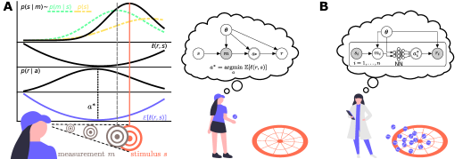
Figure 1: A Bayesian decision-making problem from the perspective of the subject. The subject needs to find the optimal action $a^{*}$ based on the sensory measurement $m$ of the state of the world $s$. Combined with a cost function $\ell(r,s)$ and the action distribution $r\sim\operatorname{\text{Lognormal}}(a,\sigma_{r})$, they want to minimize a cost function under their belief about the state of the world which yields the optimal action $a^{*}=\operatorname*{\arg\min}_{a}\operatorname{\mathbb{E}}_{p(s\>|\>m)}\left[\operatorname{\mathbb{E}}_{p(r\>|\>a)}\left[\ell(r,s)\right]\right]$. B Bayesian inference problem about the subject’s parameters from the perspective of the researcher. The researcher solves the inverse decision-making problem, i.e. they want to infer the posterior distribution $p(\theta\mid\mathcal{D})$ over the parameters $\theta$ of the subject’s perception-action system and cost function given a dataset $\mathcal{D}=\{s_{i},r_{i}:i=1,\dots,n\}$ of stimuli $s_{i}$ and responses $r_{i}$ from $n$ trials. To make inference of the posterior over $\theta$ feasible, we use a neural network as approximator for the optimal action $a^{*}$.

We start with the standard formulation of Bayesian decision theory [43], illustrated in Fig. 1 A. An actor receives a stochastic observation $m$ generated from a latent state $s$, according to a generative model $p(m\>|\>s)$. Since the actor has no direct access to the true value of the state $s$, they need to infer it by combining a prior distribution $p(s)$ with the likelihood $p(m\>|\>s)$ using Bayes’ rule

$$p(s\>|\>m)\propto p(m\>|\>s)\,p(s).$$

This Bayesian inference process describes the actor’s perception. Based on their perception, the actor’s goal is to perform an optimal action $a^{*}$, which represents the intended motor response. This is commonly framed as a decision-making problem based on a cost function $\ell(a,s)$. The optimal action $a^{*}$ for the actor is the action $a$ that minimizes the expected cost under the posterior distribution

$$a^{*} =\operatorname*{\arg\min}_{a}\operatorname{\mathbb{E}}_{p(s\>|\>m)}[\ell(a,s)]=\operatorname*{\arg\min}_{a}\int\ell(a,s)\,p(s\>|\>m)\,ds.$$ (1)

Often, the loss is not defined directly in terms of the performed action $a$, but in terms of the expectation over some stochastic version of it $r\sim p(r\>|\>a)$, modeling variability in responses with the same intended action $a$. Taking the expectation over the posterior distribution and the response distribution lets us expand Eq. 1 as

$$a^{*} =\operatorname*{\arg\min}_{a}\operatorname{\mathbb{E}}_{p(s\>|\>m)}\left[\operatorname{\mathbb{E}}_{p(r\>|\>a)}\left[\ell(r,s)\right]\right]=\operatorname*{\arg\min}_{a}\int\int\ell(r,s)\,p(r\>|\>a)\,p(s\>|\>m)\,dr\,ds,$$

which changes the problem conceptually from computing an estimate of a latent variable to performing an action that is subject to motor noise.

4 Method

The Bayesian decision-making problem in Section 3 describes the situation faced by a subject performing a task. For example, consider a subject in an experiment throwing a ball at a target. There is uncertainty in the perception of the target, which increases with the distance to the target. The subject has a prior belief about target locations, which might bias their perception. Additionally, there is uncertainty in the motor actions, such that repeated throws aimed at the same location will be variable. The task can be described by a cost function. For example, this cost function could consist of two parts. One part could be a function of the distance between the ball and the target. The other part could relate to motor effort, with throws at a larger distance being more costly. This is only an example and our framework in general allows for arbitrary parametric families of cost functions. As a Bayesian actor, the subject then chooses the action that maximizes the expected cost, taking into account the uncertainty in perception and action.

From the researcher’s perspective, want to infer the parameters of the subject’s perception-action system. In the ball throwing example, we would be interested in the subject’s perceptual uncertainty and their prior belief about the target location, their action variability, and the effort cost of throwing the ball. These parameters constitute a parameter vector ${\bm{\theta}}$. Formally, we want to compute the posterior $p({\bm{\theta}}\>|\>\mathcal{D})$ for a set $\mathcal{D}$ of behavioral data, as shown in Fig. 1 B.

Our proposed method consists of two parts. First, we approximate the optimal solution of the Bayesian decision-making problem with a neural network (Section 4.1). A forward-pass of the neural network is very fast compared to the computation of numerical solutions to the original Bayesian decision-making problem, and gradients of the optimal action w.r.t. the parameters of the model (uncertainties, priors, costs) can be efficiently computed. In the second part of our method, this allows us to utilize the neural network within a statistical model of an actor’s behavior to perform inference about model parameters (Section 4.2).

4.1 Amortizing Bayesian decision-making using neural networks

Because the Bayesian decision-making problem stated in Eq. 1 is intractable for general cost functions, we approximate it using a neural network $a^{*}\approx f_{\psi}({\bm{\theta}},m)$, which takes the parameters of the Bayesian model ${\bm{\theta}}$ and the observed variable $m$ as input and is parameterized by learnable parameters $\psi$. It can then be used as a stand-in for the computation of the optimal action $a^{*}$ in down-stream applications of the Bayesian actor model, in our case to perform inference about the Bayesian actor’s parameters.

4.1.1 Unsupervised training

We train the neural network in an unsupervised fashion by using the cost function of the decision-making problem as an unsupervised stochastic training objective. After training, the neural network implicitly solves the Bayesian decision-making problem.

More specifically, we use the expected posterior loss

$$\mathcal{L}(\psi) =\operatorname{\mathbb{E}}_{p(s\>|\>m)}\left[\operatorname{\mathbb{E}}_{p(r\>|\>f_{\psi}({\bm{\theta}},m))}\left[\ell(r,s)\right]\right]$$

as a training objective. Because the inner expectation depends on the parameters of the neural network, w.r.t. which we want to compute the gradient, we need to apply the reparameterization trick [44] and instead take the expectation over a distribution that does not depend on $\psi$

$$\mathcal{L}(\psi)=\operatorname{\mathbb{E}}_{p(s\>|\>m)}\left[\operatorname{\mathbb{E}}_{p(\epsilon)}\left[\ell\left(r,s\right)\right]\right],$$

where $r=g\left(f_{\psi}\left({\bm{\theta}},m\right),\epsilon\right)$ with some appropriate transformation $g$. For example, in the perceptual decision-making model used later (Section 5.1), $p(r\>|\>a)$ is log-normal with scale parameter $\sigma_{r}$, so we can sample $\epsilon\sim\mathcal{N}(0,1)$ and use the reparameterization $g(\epsilon,a)=\exp\left(\log(a)+\epsilon\sigma_{r}\right)$.

Now, we can easily evaluate the gradient of the objective using a Monte Carlo approximation of the two expectations,

$$\nabla_{\psi}\mathcal{L}(\psi)\approx\frac{1}{K}\frac{1}{N}\sum_{k=1}^{K}\sum_{n=1}^{N}\nabla_{\psi}\ell_{\bm{\theta}}(r_{n},s_{k}),$$

which makes it possible to train the network using any variant of stochastic gradient descent. In other words, the loss function used to train the neural network that approximates the optimal Bayesian decision-maker is simply the loss function of the underlying Bayesian decision-making problem. All that we require is a model in which it is possible to draw samples from the posterior distribution $s_{k}\sim p(s\>|\>m)$ and the response distribution $r_{n}\sim p(r\>|\>a)$. This allows us to train the network in an unsupervised fashion, i.e. we only need a training data set consisting of parameters ${\bm{\theta}}$ and inputs $m$, without the need to solve for the optimal actions beforehand. The procedure is summarized in Algorithm 1. See Section C.1 for the prior distributions used to generate parameters during training.

We used the RMSProp optimizer with a learning rate of $10^{-4}$, batch size of 256, and N = M = 128 Monte Carlo samples per evaluation of the stochastic training objective. The networks were trained for 500,000 steps, and we assessed convergence using an evaluation set of analytically or numerically solved optimal actions (see Section C.2).

4.1.2 Network architecture

We used a multi-layer perceptron with 4 hidden layers and 16, 64, 16, 8 nodes in the hidden layers, respectively. We used swish activation functions at the hidden layers [45]. As the final layer, we used a linear function with an output $\mathbf{y}\in\mathbb{R}^{3}$, followed by a non-linearity $a^{*}=\text{softplus}(y_{1}m^{y_{2}}+y_{3})$, where $m$ is the observation received by the subject. This particular non-linearity is motivated by the functional form of the analytical solution of the Bayesian decision-making problem for the quadratic cost function as a function of $m$ and ${\bm{\theta}}$ (Section 5.1) and serves as an inductive bias (Section C.3).

4.2 Bayesian inference of model parameters

The graphical model in Fig. 1 B illustrates the generative model of behavior in an experiment. Our goal is to infer $p({\bm{\theta}}\>|\>\mathcal{D})$, where $\mathcal{D}=\{s_{i},r_{i}:i=1,\dots,n\}$ is a dataset of stimuli and responses. We assume that for every stimulus $s$ presented to the subject, they receive a stochastic measurement $m\sim p(m\>|\>s)$. They then solve the Bayesian decision problem given above, i.e. they decide on an action $a$. We used the neural network $a^{*}\approx f(m,{\bm{\theta}})$ to approximate the optimal action. The chosen action is then corrupted by action variability to yield a response $r\sim p(r\>|\>a)$. To sample from the researcher’s posterior distribution over the subject’s model parameters $p({\bm{\theta}}\>|\>\mathcal{D})$, we use the Hamiltonian Monte Carlo algorithm NUTS [46]. This gradient-based inference algorithm can be used because the neural network is differentiable with respect to the parameters ${\bm{\theta}}$ and sensory input $m$. The procedure is summarized in Algorithm 2.

4.3 Implementation

The method was implemented in jax [47], using the packages equinox [48] for neural networks and numpyro [49] for probabilistic models and sampling. Our implementation is provided in the supplementary material and will be made available on GitHub upon publication. Our software package enables the user to define new, arbitrary parametric families cost functions and train neural networks to approximate the decision-making problem.

No special high-performance compute resources were needed, since all evaluations for this paper were run on standard laptop computers (e.g. with Intel Core i7-8565U CPU). Training a neural network for 500,000 steps took 10 minutes, and drawing 20,000 posterior samples for a typical dataset with 60 trials took 10 seconds.

5 Results

We evaluate our method on a perceptual decision-making task with log-normal prior, likelihood and action distribution (Section 5.1), which we later combine with several cost functions. For certain cost functions, this Bayesian decision-making problem is analytically solvable. We evaluate our method’s posterior distributions against those obtained when using the analytical solution for the optimal action (Section 5.2). Our evaluations allowed us to find possible identifiability problems between prior and cost parameters inherent to Bayesian actor models, which we analyze in more detail (Section 5.3). Finally, we apply our method to real data from a sensorimotor task performed by humans and show that it explains the variability and biases in the data (Section 5.4).

5.1 Perceptual decision-making model

We now make the decision-making problem more concrete by introducing a log-normal model for the perceptual and action uncertainties, which captures the ball throwing example sketched in Section 4 and shown in Fig. 2. From the actor’s perspective, we assume that sensory measurements are generated from a log-normal distribution $m\sim\operatorname{\text{Lognormal}}(m\>|\>s,\sigma)$, or equivalently that $\ln m\sim\mathcal{N}(m\>|\>\ln s,\sigma)$. This assumption is motivated by Weber’s law, i.e. that the variability scales linearly with the mean [15], and by Fechner’s law, i.e. that perception takes place on an internal logarithmic scale [50]. Thus, this model can be applied to a wide range of stimuli, such as time [51, 52], space [53], sound [54], numerosity [52, 53, 55], and others.

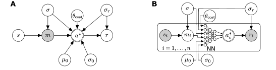
Figure 2: The graphical models from Fig. 1 with specific parameters for the log-normal perceptual decision-making model described in Section 5.1. The parameters represent the perceptual uncertainty $\sigma$, the motor variability $\sigma_{r}$ and the log-normal prior defined by $(\mu_{0},\sigma_{0})$. The parameter vector $\theta_{\text{cost}}$ is defined by the employed cost function. E.g., for quadratic cost without any free parameters, $\theta_{\text{cost}}=\{\varnothing\}$, or for costs function incorporating cost parameters in equations (3) and (4), it is $\theta_{\text{cost}}=\{\beta\}$ and $\theta_{\text{cost}}=\{\alpha\}$, respectively. A Subject view of the task. B Model from the researcher’s perspective.

Posterior distribution

Assuming a log-normal prior $s\sim\operatorname{\text{Lognormal}}(\mu_{0},\sigma_{0})$ and a log-normal likelihood $m\sim\operatorname{\text{Lognormal}}(s,\sigma)$, the posterior is

$$p(s\>|\>m)=\operatorname{\text{Lognormal}}(\mu_{\text{post}},\sigma_{\text{post}})$$ (2)

with $\sigma_{\text{post}}^{2}=(\frac{1}{\sigma_{0}^{2}}+\frac{1}{\sigma^{2}})^{-1}$ and $\mu_{\text{post}}=\exp\left(\sigma_{\text{post}}^{2}\left(\frac{\ln\mu_{0}}{\sigma_{0}^{2}}+\frac{\ln m}{\sigma^{2}}\right)\right)$. This can be shown by using the equations for Gaussian conjugate priors for a Gaussian likelihood in logarithmic space and then converting back to the original space.

Response distribution

Motivated by the idea of signal-dependent noise in actions [14], we again use a log-normal distribution $r\sim\operatorname{\text{Lognormal}}(r\>|\>a,\sigma_{r})$ as a probability distribution describing the variability of responses $r$ given an intended action $a$. This assumption results in a linear scaling of response variability with the mean, which has been observed empirically [56, 57].

Analytical solution for quadratic costs

For certain cost functions, this formulation allows analytical solutions for the optimal action. Specifically, for quadratic costs $\ell(r,s)=(r-s)^{2}$, the optimal action is $a^{*}=\mu_{\text{post}}\,\exp\left(\frac{1}{2}\left(\sigma_{\text{post}}^{2}-3\sigma_{r}^{2}\right)\right)$. For a derivation, see Section B.1. This allows us to validate our method against a special case in which the optimal action can be computed analytically.

5.2 Evaluation using synthetic data

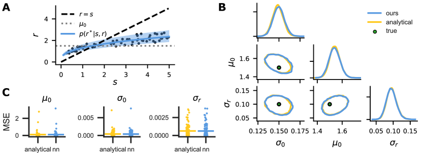
Figure 3: A Simulated data from the Bayesian actor model with quadratic cost function are shown as a scatter plot. The posterior predictive distribution (mean and 94% CI) obtained using our method is shown as a blue line with shaded region. B Posterior distributions of parameters obtained using the analytical solution or the neural network to compute optimal actions. Ground truth parameter values are shown for comparison. C Evaluation (MSE between posterior mean and ground truth) for multiple runs with uniformly sampled ground truth parameters.

We first evaluate our method on a case for which we know the analytical solution for the optimal action: the quadratic cost function (Section 5.1). We generated a dataset of 60 pairs of stimuli $s_{i}$ and responses $r_{i}$ using the analytical solution for the optimal action with ground truth parameters $\mu_{0}=1.5,\sigma_{0}=0.15,\sigma=0.2,\sigma_{r}=0.1$. The simulated data are shown in Fig. 3 A, with a characteristic pattern of signal-dependent increase in variability, an overshot for low stimulus values and an undershot for higher stimulus values due to the prior. We then computed posterior distributions for the model parameters using the analytical solution for the optimal action and using the neural network. We drew 20,000 samples from the posterior distribution in 4 chains, each warmed up with 5,000 burn-in steps. Note that, because the concrete values of $\sigma$ and $\sigma_{0}$ are unidentifiable even when using the analytical solution for the optimal action (see Section D.1), we kept $\sigma$ fixed to its true value during inference. This was done to evaluate our method on a version of the model, for which the analytical solution as a gold standard produces reliable results. Fig. 3 B shows that both versions recover the true parameters, and the contours of both posteriors align well. The posterior predictive distribution generated from the neural network posterior reproduces the pattern of variability and bias in the data (shaded region in Fig. 3 A).

To ensure and quantitatively assess that the method works for a wide range of parameter settings, we then simulated 100 sets of parameters sampled uniformly (see Section C.1 for the choice of prior distributions). For each set of parameters, we simulated a dataset consisting of 60 trials. We then computed posterior distributions for each dataset in two ways: using the analytical solution for the optimal action and using the neural network to approximate the optimal action. In both cases, we drew 20,000 samples (after 5,000 warm-up steps) from the posterior distribution in 4 chains and assessed convergence by checking that the R-hat statistic [58] was below 1.05. The mean squared errors between the posterior mean and the ground truth parameter value in Fig. 3 C show that the inference method using the neural network recovers the ground truth parameters just as well as the analytical version. Fig. D.2 A&B additionally show the error as a function of the ground truth parameter value and Table D.1 shows the results from Fig. 3 C numerically.

5.3 Limits of identifiability of costs and priors

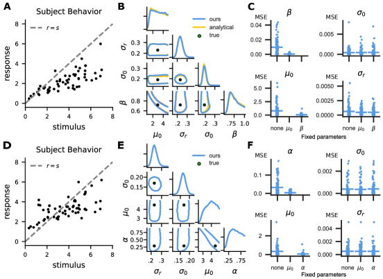
Figure 4: A Example of behavior simulated from the quadratic cost function with effort cost (Eq. 3). The responses exhibit undershots, which could either be due to the prior or due to the cost. B Posteriors with the analytical model versus the neural network model over the parameter set from panel A. For each pair of parameters, the plot shows the contours of the 94%-HDI. Our method approximates the posterior with the analytical solution quite well and mimics its behavior regarding the uncertainty over different parameters. The pairwise posterior between prior mean $\mu_{0}$ and effort cost parameter $\beta$ shows a strong correlation. C MSE between ground truth and posterior mean when fixing no parameters, the effort parameter $\beta$ or the prior parameter $\mu_{0}$. Fixing one of the confounding variables results in a considerable improvement of accuracy in the inference of the non-fixed variable. The other parameters maintain their accuracy. D-F Same as A-C, but for asymmetric quadratic cost (Eq. 4), with no analytical solution. In the asymmetric quadratic cost function, parameter $\alpha$ controls the influence of effort cost and thus correlates with the prior parameter $\mu_{0}$.

We now apply our method to new cost functions, for which analytical solutions are not (readily) available. For example, we consider cost functions that incorporate the cost of the effort of actions. It is more costly to throw a ball at a longer distance due to the force needed to produce the movement, or it is more effortful to press a button for a longer duration. This can be achieved using a weighted sum of the squared distance to the target stimulus and the square of the response:

$$\ell(r,s)=\beta(s-r)^{2}+(1-\beta)r^{2}.$$ (3)

This cost function introduces another source of biases besides perceptual priors: people might undershoot stimuli at larger distances more (see Fig. 4). Using our method, we can turn to investigating whether we can tease these different sources of biases apart. Fig. 4 A shows a pattern of behavior with an undershot with ground truth parameters $\mu_{0}=2.95,\sigma_{0}=0.19,\sigma=0.14,\sigma_{r}=0.23,\beta=0.72$. The posterior distribution Fig. 4 B shows that the undershot can either be attributed to a subject trying to avoid the mental or physical strain of larger effort, or to biased perception due to a low prior mean. This is difficult to disentangle, and shows in a correlated posterior for the effort cost parameter $\beta$ and the prior mean $\mu_{0}$. Over 100 simulated datasets with a range of different ground truth parameter values, the MSE between the inferred posterior mean and the ground truth is high when both $\mu_{0}$ and $\beta$ are unknown. Once we fix one of the confounding parameters at their true value and exclude them from the set of inferred parameters, we observe a considerable increase in accuracy of the inferred parameters (see Fig. 4 C). Again, Fig. D.2 C&D show the error as a function of the ground truth parameter value and Table D.2 shows the results from Fig. 4 C numerically.

Nevertheless, this unidentifiability is a property of the model itself and not a shortcoming of the inference method. In fact, our method opens up the possibility to investigate these properties of Bayesian actor models in the first place. To demonstrate this, we derived an analytical solution for the quadratic cost with quadratic effort (see Section B.2) and showed that the posteriors obtained using the neural network match those obtained with the analytical solution (see Fig. 4 B).

We performed the same analysis for an asymmetric quadratic cost function, which can penalize overshots more than undershots, or vice versa:

$$\ell(r,s)=2|\alpha-\mathds{1}(r-s)|(r-s)^{2}\quad\text{with}\quad\mathds{1}(x)=\begin{cases}1&\quad\text{if}\quad x\geq 0\\ 0&\quad\text{else}\\ \end{cases}.$$ (4)

Fig. 4 D shows an example of behavior generated using this cost function with $\mu_{0}=4.47,\sigma_{0}=0.17,\sigma=0.22,\sigma_{r}=0.23$ and $\alpha=0.29$, which exhibits an undershot. There is no analytical solution for the Bayesian decision-making problem with this cost function known to us. Nevertheless, ground truth parameters are accurately inferred (see Fig. 4 E) and the same pattern of identifiability issues as for the previous cost function is observed (see Fig. 4 F and Table D.3).

5.4 Inference of human costs and priors

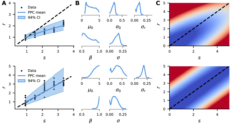
Figure 5: A Data from two subjects in a bean-bag throwing task [59], along with posterior predictive distributions (mean and 94% CI) obtained using our method. B Marginal posterior distributions (KDE) for both participants. C Posterior mean cost functions plotted as a color map in stimulus-response space (high cost to low cost from red to blue).

We applied our method to data of human participants from a previously published study of a bean bag throwing task [59]. 20 participants were asked to throw a bean bag at five different target distances from 3 to 11 feet (0.9 to 3.4 meters) with 2 feet increments (0.6 meters). The subjects received neither visual nor verbal feedback. Fig. 5 A shows data from two example participants from the study. The first participant’s behavior is characterized by a tendency to undershoot far targets. The second participant hits the target accurately on average, but has a higher variability.

We fit the model using the quadratic cost function with quadratic effort to the data by drawing 20,000 samples (after 5,000 warm-up steps) from the posterior distribution for both participants. The posterior distributions (Fig. 5 B) show that the first participant’s behavior can be either explained by an effort cost or a prior belief about targets (either low $\beta$ or low $\mu_{0}$), but we cannot conclusively say which of the two is the case (cf. Section 5.3). The second participant’s relatively unbiased behavior is attributed to a comparatively small effort cost, with $\beta$ being very close to 1. The action variability $\sigma_{r}$ is higher compared to the first participant.

The posterior mean cost function is visualized in the two-dimensional target-response space in Fig. 5 C, where the color indicates the cost of performing a response $r$ when the target is $s$. For the first participant, the cost function exhibits an asymmetry: for targets that are further away, the minimum of the cost function is shifted towards shorter responses. The second participant’s cost function, on the other hand, is symmetric around the target.

6 Discussion

First, we have presented a new framework for Bayesian inference about the parameters of Bayesian actor models. Computing optimal actions in these models is intractable for general cost functions and, therefore, previous work has often focused on cost functions with analytical solutions, or derived custom tools for specific tasks. We propose an unsupervised training scheme for neural networks to approximate Bayesian actor models with general parametric cost functions. The approach is extensible to cost functions with other functional forms suited to particular tasks. Second, performing inference about the parameters of Bayesian actor models given behavioral data is computationally very expensive because each evaluation of the likelihood requires solving the decision-making problem. By plugging in the neural network approximation, we can perform efficient inference. Third, a very large number of tasks involve continuous responses, including economic decision-making (‘how much would you wager in a bet?’), psychophysical production (‘hit the target’), magnitude reproduction (‘reproduce the duration of a tone’), sensorimotor tasks (‘reproduce the force you felt’), and cross-modality matching (‘adjust a sound to appear as loud as the brightness of this light’). Therefore we see very broad applicability of our method in the behavioral sciences including cognitive science, psychology, neuroscience, sensorimotor control, and behavioral economics. Fourth, over the last few years, a greater appreciation of the necessity for experiments with continuous responses has developed [60]. Such decision problems are closer to natural environments than discrete forced-choice decisions, which have historically been the dominant approach. We provide a statistical method for analyzing continuous responses. Finally, by inferring what a subject’s decisions were optimal for instead of postulating optimality, we conceptually reconcile normative and descriptive models of decision-making. Thus, we model the researcher’s uncertainty about the subject’s decision-making parameters explicitly.

Once we move beyond quadratic cost functions, identifiability issues between prior and cost parameters can arise. As recognized in other work as well [37, 36], these identifiability issues in Bayesian models have implications for how experiments should be designed. We have shown that, when either priors or costs are known, the identifiability issue vanishes. Based on our results, we recommend experiments with multiple conditions, between which one can assume either priors or costs to stay fixed, in order to disentangle their effects. Our methodology should prove particularly useful for investigating task configurations that lead to or avoid such unidentifiabilities.

Limitations

The strongest limitation we see with the present approach is that we require a model of the perceptual problem that allows drawing samples from the observer’s posterior distribution, which works for stimuli that can be described well by these assumptions, e.g. magnitude-like stimuli with log-normal distributions considered in our experiments. Ideally, we would like a method that can be applied to perceptual stimuli for which these assumptions do not hold (e.g. circular variables) or more complex cognitive reasoning tasks. We see a potential to extend our method by learning an approximate posterior distribution together with the action network. This idea is closely related to loss-calibrated inference [61, 62], an approach that learns variational approximations to posterior distribution adapted to loss functions. We will explore this connection more in future work.

Broader impacts

Methods for inferring beliefs and costs from behavioral data have potential for both positive and negative societal impact. We see a great benefit for behavioral research from methods that provide estimates of people’s perceptual, motor, and cognitive properties from continuous action data, particularly in clinical applications where such tasks are easier for patients than classical forced-choice tasks. On the other hand, methods to infer people’s uncertainties and costs could potentially be used in harmful ways, especially if they are used without the subjects’ consent. The inference methods presented here are applicable to controlled experiments, and are far from scenarios with harmful societal outcomes. Still, applications of these methods should of course take place with the subjects’ informed consent and the oversight of ethical review boards.

Appendix A Algorithm

0:  Trained neural network $f_{\psi}({\bm{\theta}},m)\approx\operatorname*{\arg\min}_{a}\operatorname{\mathbb{E}}_{p(s\>|\>m)}\left[\operatorname{\mathbb{E}}_{p(r\>|\>a)}\left[\ell(r,s)\right]\right]$

0:  Researcher’s prior distribution for training the neural network $p({\bm{\theta}})$,
Subject’s perceptual model $p_{\bm{\theta}}(m\>|\>s)$ and $p_{\bm{\theta}}(s)$,
Subject’s response model $p_{\bm{\theta}}(r\>|\>a)$,
Subject’s cost function $\ell_{\bm{\theta}}(r,s)$

1:  while test error $>$ desired test error do

2:     Draw ${\bm{\theta}}\sim p({\bm{\theta}})$

3:     Compute expected loss $\mathcal{L}(\psi)=\operatorname{\mathbb{E}}_{p_{\bm{\theta}}(s\>|\>m)}\left[\operatorname{\mathbb{E}}_{p(\epsilon)}\left[\ell_{\bm{\theta}}\left(r,s\right)\right]\right]\approx\frac{1}{K}\frac{1}{N}\sum_{k=1}^{K}\sum_{n=1}^{N}\ell_{\bm{\theta}}(r_{n},s_{k})$

4:     Perform gradient descent step with $\nabla_{\psi}\mathcal{L}(\psi)\approx\frac{1}{K}\frac{1}{N}\sum_{k=1}^{K}\sum_{n=1}^{N}\nabla_{\psi}\ell_{\bm{\theta}}(r_{n},s_{k})$

5:     Evaluate error of optimal actions on an evaluation set (see Section C.2)

6:  end while

Algorithm 1 Train neural network to approximate a Bayesian actor model

0:  Samples from posterior distribution $p({\bm{\theta}}\>|\>\mathcal{D})$

0:  Researcher’s prior distribution $p({\bm{\theta}})$,
Data $\mathcal{D}=\{s_{i},r_{i}:i=1,\dots,n\}$,
Subject’s perceptual model $p_{\bm{\theta}}(m\>|\>s)$ and $p_{\bm{\theta}}(s)$,
Subject’s response model $p_{\bm{\theta}}(r\>|\>a)$,
Subject’s cost function $\ell_{\bm{\theta}}(r,s)$

1:  Obtain pre-trained neural network $a=f_{\psi}({\bm{\theta}},m)$ from Algorithm 1

2:  Sample from the posterior $p({\bm{\theta}}\>|\>\mathcal{D})$ defined by the graphical model Fig. 1 C using NUTS

Algorithm 2 Bayesian inference about the parameters of a Bayesian actor model

Appendix B Derivations of optimal actions

B.1 Quadratic cost

One cost function for which the Bayesian decision-making problem under a log-normal observation model and a log-normal response model (Section 5.1) can be solved in closed form is the quadratic function. In that case, we can write the expected loss as

$$\operatorname{\mathbb{E}}\left[\ell(r,s)\right] =\operatorname{\mathbb{E}}\left[(s-r)^{2}\right]$$

$$=\operatorname{\mathbb{E}}\left[s^{2}\right]-2\operatorname{\mathbb{E}}\left[s\right]\operatorname{\mathbb{E}}\left[r\right]+\operatorname{\mathbb{E}}\left[r^{2}\right],$$

assuming independence between $s$ and $r$.

Using the moment-generating function of the log-normal distribution, we can evaluate these expectations as

$$\operatorname{\mathbb{E}}\left[\ell(r,s)\right] =e^{2\ln\mu_{\text{post}}+2\sigma_{\text{post}}^{2}}-2e^{\ln\mu_{\text{post}}+\frac{\sigma_{\text{post}}^{2}}{2}}e^{\ln a+\frac{\sigma_{r}^{2}}{2}}+e^{2\ln a+2\sigma_{r}^{2}}.$$

By differentiating with respect to $a$

$$\frac{\partial}{\partial a}\operatorname{\mathbb{E}}\left[\ell(r,s)\right]=2e^{2\sigma_{r}^{2}}a-2\mu_{\text{post}}e^{\frac{1}{2}(\sigma_{r}^{2}+\sigma_{\text{post}}^{2})}$$

and setting to zero, we obtain the optimal action

$$a^{*}=\mu_{\text{post}}\,\exp\left(\frac{1}{2}\left(\sigma_{\text{post}}^{2}-3\sigma_{r}^{2}\right)\right).$$

Inserting the posterior mean (Eq. 2), we obtain

$$\begin{split}a^{*}&=\exp\left(\sigma_{\text{post}}^{2}\left(\frac{\ln\mu_{0}}{\sigma_{0}^{2}}+\frac{\ln m}{\sigma^{2}}\right)\right)\,\exp\left(\frac{1}{2}\left(\sigma_{\text{post}}^{2}-3\sigma_{r}^{2}\right)\right)\\ &=\mu_{0}^{\frac{\sigma_{\text{post}}^{2}}{\sigma_{0}^{2}}}\exp\left(\frac{1}{2}\left(\sigma_{\text{post}}^{2}-3\sigma_{r}^{2}\right)\right)\,m^{\frac{\sigma_{\text{post}}^{2}}{\sigma^{2}}}\end{split}$$ (5)

B.2 Quadratic cost with quadratic action effort

We now consider a class of cost functions of the form

$$\ell(r,s)=\beta(s-r)^{2}+(1-\beta)r^{2}.$$

This allows us to write the expected cost as

$$\operatorname{\mathbb{E}}\left[\ell(r,s)\right] =\operatorname{\mathbb{E}}\left[\beta(s-r)^{2}+(1-\beta)r^{2}\right]$$

$$=\beta\operatorname{\mathbb{E}}\left[(s-r)^{2}\right]+(1-\beta)\operatorname{\mathbb{E}}\left[r^{2}\right]$$

Using the previously obtained result of Section B.1, we can write this as

$$\operatorname{\mathbb{E}}\left[\ell(r,s)\right] =\beta\left(e^{2\ln\mu_{\text{post}}+2\sigma_{\text{post}}^{2}}-2e^{\ln\mu_{\text{post}}+\frac{\sigma_{\text{post}}^{2}}{2}}e^{\ln a+\frac{\sigma_{r}^{2}}{2}}+e^{2\ln a+2\sigma_{r}^{2}}\right)+(1-\beta)e^{2\ln a+2\sigma_{r}^{2}}.$$

Differentiating

$$\frac{\partial}{\partial a}\operatorname{\mathbb{E}}\left[\ell(r,s)\right]=2e^{2\sigma_{r}^{2}}a-2\beta\mu_{\text{post}}e^{\frac{1}{2}(\sigma_{r}^{2}+\sigma_{\text{post}}^{2})}$$

and setting to zero as well as inserting the posterior mean (Eq. 2) yields

$$a =\beta\mu_{\text{post}}\exp\left(\frac{1}{2}\left(\sigma_{\text{post}}^{2}-3\sigma_{r}^{2}\right)\right)$$

$$=\beta\exp\left(w_{0}\ln\mu_{0}+\frac{\sigma_{\text{post}}^{2}}{2}-\frac{3\sigma_{r}^{2}}{2}\right)\,m^{w_{m}}$$

with $w_{0}=\frac{\sigma_{\text{post}}^{2}}{\sigma_{0}^{2}}$ and $w_{m}=\frac{\sigma_{\text{post}}^{2}}{\sigma^{2}}$.

Appendix C Hyperparameters and other methods details

C.1 Parameter prior distributions

We use relatively wide priors to generate the training data for the neural networks to ensure that they accurately approximate the optimal action over a wide range of possible parameter values:

• $\sigma\sim\mathcal{U}(0.01,0.5)$

• $\sigma_{r}\sim\mathcal{U}(0.01,0.5)$

• $\sigma_{0}\sim\mathcal{U}(0.01,0.5)$

• $\mu_{0}\sim\mathcal{U}(0.1,7.0)$

During inference, we use narrower, but still relatively uninformed prior distributions, to avoid the regions of the parameter space on which the neural network has not been trained:

• $\sigma\sim\text{Half-Normal}(.25)$

• $\sigma_{r}\sim\text{Half-Normal}(.25)$

• $\sigma_{0}\sim\text{Half-Normal}(.25)$

• $\mu_{0}\sim\mathcal{U}(0.1,5.0)$

To evaluate the inference procedure, we use parameters sampled from priors, which correspond to the actual parameter values that we would in expect in a behavioral experiment:

• $\sigma\sim\mathcal{U}(0.1,0,25)$

• $\sigma_{r}\sim\mathcal{U}(0.1,0,25)$

• $\sigma_{0}\sim\mathcal{U}(0.1,0,25)$

• $\mu_{0}\sim\mathcal{U}(2.0,5.0)$

In contrast to the sensorimotor parameters, we kept the same priors for cost parameters during training of the neural network, inference and evaluation:

• Quadratic cost with linear effort: $\beta\sim\mathcal{U}(0.5,1.0)$

• Quadratic cost with quadratic effort: $\beta\sim\mathcal{U}(0.5,1.0)$

• Asymmetric quadratic cost: $\alpha\sim\mathcal{U}(0.1,0.9)$

C.2 Evaluation dataset

To assess convergence of the neural networks, we generated an evaluation dataset consisting of 100,000 parameter sets and optimal solutions of the Bayesian decision-making problem for each cost function. If an analytical solution was available (e.g. quadratic cost), we computed the optimal action analytically. If there was no analytical solution known to us, we solved the Bayesian decision-making problem numerically. Specifically, we computed Monte Carlo approximations of the posterior expected loss

$$\mathcal{L}(a) =\operatorname{\mathbb{E}}_{p(s\>|\>m)}\left[\operatorname{\mathbb{E}}_{p(r\>|\>a))}\left[\ell(r,s)\right]\right]$$

$$\approx\frac{1}{K}\frac{1}{N}\sum_{k=1}^{K}\sum_{n=1}^{N}\ell(r_{n},s_{k})$$

with $N=K=10,000$ and used the BFGS optimizer (implemented in jax.scipy) to solve for the optimal action $a^{*}$.

C.3 Inductive bias for the neural network

We know the closed-form solution for the optimal action $a^{*}$ as a function of the parameters ${\bm{\theta}}$ for the quadratic cost function (Section B.1). Therefore, we assume that the parametric form of the optimal action as a function of the sensory measurement $m$ will not be substantially different for other cost functions, although the specific dependence on the parameters will vary. We rewrite the optimal action for the quadratic loss (Eq. 5) as

$$a^{*}=f_{1}({\bm{\theta}})m^{f_{2}({\bm{\theta}})}+f_{3}({\bm{\theta}}).$$

To allow for additive biases as well, we have added an additive term, which is zero for the quadratic cost function.

Appendix D Additional results

D.1 Inference with both perceptual and prior uncertainty as free parameters

During evaluation of our method, we found identifiability issues inherent to Bayesian actor models between the prior uncertainty $\sigma_{0}$ and the sensory variability $\sigma$. In order to produce the same behavior as the one observed, only the ratio $\frac{\sigma_{0}}{\sigma}$ needs to be inferred correctly (see diagonal correlation in the joint posterior of the two parameters in Fig. D.1 A) – the absolute magnitude of each of the two parameters does not substantially influence the resulting behavior and thus the solution to the true values conditioned on the observed behavior is an underdetermined problem. This intuitively makes sense, since the resulting behavior is largely shaped by how much influence prior and sensory information have, which is weighted by $\sigma_{0}$ and $\sigma$, respectively.

We were able to considerably improve accuracy in the inference of these two confounding parameters by fixing one of them at their true value (see Fig. D.1 B). Therefore, we decided to keep the perceptual uncertainty $\sigma$ fixed when probing our method since this corresponds to psychophysically measuring $\sigma$ prior to applying our method and fixing it at the measure value.

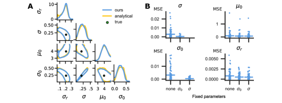
Figure D.1: A Posteriors with the analytical model versus the neural network model for an arbitrary, synthetically generated data set that captures the identifiability problem between $\sigma$ and $\sigma_{0}$ quite clearly. Our method approximates the posterior with the analytical solution quite well and mimics its behavior regarding the uncertainty over different parameters. The pairwise posterior between prior uncertainty $\sigma_{0}$ and perceptual uncertainty $\sigma$ shows a strong correlation. B MSE when fixing no parameters, the perceptual uncertainty $\sigma_{0}$ or the prior parameter $\sigma$. Fixing one of the confounding variables results in a considerable improvement of accuracy in the inference of the non-fixed parameter. The prior parameter $\mu_{0}$ maintains its accuracy while the errors for the response variability $\sigma_{r}$ also slightly decrease.

D.2 Accuracy of inference with amortized optimal actions

D.2.1 Comparison of posterior means and standard deviations

To assess the accuracy of the inference with amortized optimal actions, we used the data sets also shown in Fig. 3 C and Fig. 4 C. We compared means and standard deviations of the posteriors obtained with the analytical solutions for the optimal actions $a^{*}$ or with the neural network as approximation for the subject’s decision-making. The neurally amortized inference accurately produces very similar posteriors to the ones obtained using the analytical solution, as shown in Fig. D.2.

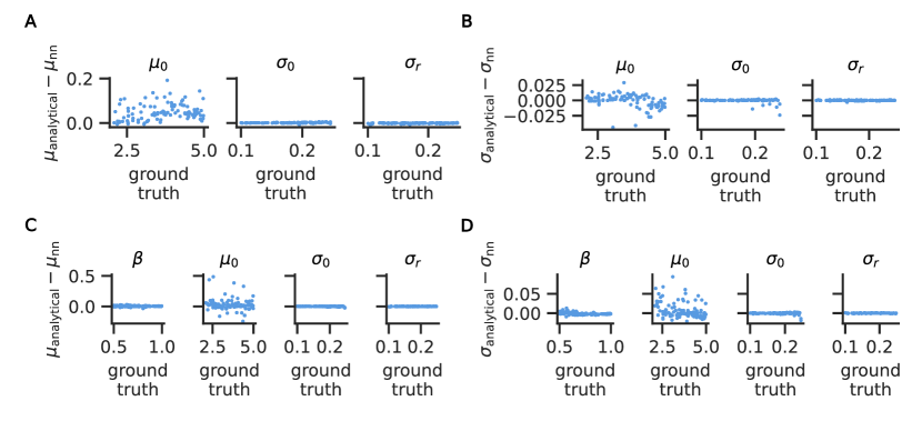
Figure D.2: Error between posteriors as a function of ground truth parameter values. For each simulated data set in our evaluation (Fig. 3 C and Fig. 4 C), we computed the difference between posterior means and standard deviations for posterior distributions obtained using analytical optimal actions and our neural network approximations. A Difference between posterior means for quadratic cost. B Difference between posterior standard deviations for quadratic cost. C Difference between posterior means for quadratic cost with quadratic effort. D Difference between posterior standard deviations for quadratic cost with quadratic effort.

D.2.2 Mean squared errors

We additionally summarize the mean squared errors visualized in Fig. 3 C (Table D.1), Fig. 4 C (Table D.2), and Fig. 4 F (Table D.3).

	MSE
Parameter	analytical	NN
$\mu_{0}$	0.10	0.10
$\sigma_{0}$	$3.98\times 10^{-4}$	$3.77\times 10^{-4}$
$\sigma_{r}$	$6.23\times 10^{-4}$	$6.13\times 10^{-4}$

Table D.1: Summary of results for quadratic cost function from Fig. 3 C. Each entry shows the mean squared error (MSE) between the posterior means and ground truth parameters, obtained using the analytical vs. neural network optimal action.

	MSE
Parameter	analytical	NN
$\mu_{0}$	0.74	0.77
$\sigma_{0}$	$3.63\times 10^{-4}$	$4.08\times 10^{-4}$
$\sigma_{r}$	$4.87\times 10^{-4}$	$4.86\times 10^{-4}$
$\beta$	$8.97\times 10^{-4}$	$8.97\times 10^{-3}$

Table D.2: Summary of results for quadratic cost with quadratic effort from 4 C. Each entry shows the mean squared error (MSE) between the posterior means and ground truth parameters, obtained using the analytical vs. neural network optimal action.

Parameter	MSE (NN)
$\mu_{0}$	0.34
$\sigma_{0}$	$3.87\times 10^{-4}$
$\sigma_{r}$	$5.05\times 10^{-4}$
$\alpha$	$3.23\times 10^{-2}$

Table D.3: Summary of results for asymmetric quadratic cost 4 F. Each entry shows the mean squared error (MSE) between the posterior means and ground truth parameters, obtained using the neural network optimal action.

References

- Ma [2019] Wei Ji Ma. Bayesian decision models: A primer. Neuron, 104(1):164–175, 2019.
- Weiss et al. [2002] Yair Weiss, Eero P Simoncelli, and Edward H Adelson. Motion illusions as optimal percepts. Nature neuroscience, 5(6):598–604, 2002.
- Ernst and Banks [2002] Marc O Ernst and Martin S Banks. Humans integrate visual and haptic information in a statistically optimal fashion. Nature, 415(6870):429–433, 2002.
- Wei and Stocker [2015] Xue-Xin Wei and Alan A Stocker. A bayesian observer model constrained by efficient coding can explain’anti-bayesian’percepts. Nature neuroscience, 18(10):1509–1517, 2015.
- Kersten et al. [2004] Daniel Kersten, Pascal Mamassian, and Alan Yuille. Object perception as bayesian inference. Annu. Rev. Psychol., 55:271–304, 2004.
- Körding and Wolpert [2004] Konrad P Körding and Daniel M Wolpert. Bayesian integration in sensorimotor learning. Nature, 427(6971):244–247, 2004.
- Todorov and Jordan [2002] Emanuel Todorov and Michael I Jordan. Optimal feedback control as a theory of motor coordination. Nature neuroscience, 5(11):1226–1235, 2002.
- Griffiths and Tenenbaum [2006] Thomas L Griffiths and Joshua B Tenenbaum. Optimal predictions in everyday cognition. Psychological science, 17(9):767–773, 2006.
- Xu and Tenenbaum [2007] Fei Xu and Joshua B Tenenbaum. Word learning as bayesian inference. Psychological Review, 114(2):245, 2007.
- Behrens et al. [2007] Timothy EJ Behrens, Mark W Woolrich, Mark E Walton, and Matthew FS Rushworth. Learning the value of information in an uncertain world. Nature neuroscience, 10(9):1214–1221, 2007.
- Berkes et al. [2011] Pietro Berkes, Gergő Orbán, Máté Lengyel, and József Fiser. Spontaneous cortical activity reveals hallmarks of an optimal internal model of the environment. Science, 331(6013):83–87, 2011.
- Van Beers et al. [2004] Robert J. Van Beers, Patrick Haggard, and Daniel M. Wolpert. The Role of Execution Noise in Movement Variability. Journal of Neurophysiology, 91(2):1050–1063, 2004.
- Trommershäuser et al. [2008] Julia Trommershäuser, Laurence T Maloney, and Michael S Landy. Decision making, movement planning and statistical decision theory. Trends in cognitive sciences, 12(8):291–297, 2008.
- Harris and Wolpert [1998] Christopher M Harris and Daniel M Wolpert. Signal-dependent noise determines motor planning. Nature, 394(6695):780–784, 1998.
- Weber [1831] Ernst Heinrich Weber. De Pulsu, resorptione, auditu et tactu: Annotationes anatomicae et physiologicae. Koehler, 1831.
- Körding and Wolpert [2004] Konrad Paul Körding and Daniel M. Wolpert. The loss function of sensorimotor learning. Proceedings of the National Academy of Sciences, 101(26):9839–9842, 2004.
- Sims [2015] Chris R Sims. The cost of misremembering: Inferring the loss function in visual working memory. Journal of vision, 15(3):2–2, 2015.
- Lewis et al. [2014] Richard L Lewis, Andrew Howes, and Satinder Singh. Computational rationality: Linking mechanism and behavior through bounded utility maximization. Topics in cognitive science, 6(2):279–311, 2014.
- Lieder and Griffiths [2020] Falk Lieder and Thomas L Griffiths. Resource-rational analysis: Understanding human cognition as the optimal use of limited computational resources. Behavioral and brain sciences, 43:e1, 2020.
- Gershman et al. [2015] Samuel J Gershman, Eric J Horvitz, and Joshua B Tenenbaum. Computational rationality: A converging paradigm for intelligence in brains, minds, and machines. Science, 349(6245):273–278, 2015.
- Hoppe and Rothkopf [2016] David Hoppe and Constantin A Rothkopf. Learning rational temporal eye movement strategies. Proceedings of the National Academy of Sciences, 113(29):8332–8337, 2016.
- Straub and Rothkopf [2022] Dominik Straub and Constantin A Rothkopf. Putting perception into action with inverse optimal control for continuous psychophysics. Elife, 11:e76635, 2022.
- Feldman [2013] Jacob Feldman. Tuning your priors to the world. Topics in cognitive science, 5(1):13–34, 2013.
- Simon [1955] Herbert A Simon. A behavioral model of rational choice. The quarterly journal of economics, pages 99–118, 1955.
- Anderson [1991] John R Anderson. Is human cognition adaptive? Behavioral and brain sciences, 14(3):471–485, 1991.
- Aitchison et al. [2015] Laurence Aitchison, Dan Bang, Bahador Bahrami, and Peter E Latham. Doubly bayesian analysis of confidence in perceptual decision-making. PLoS computational biology, 11(10):e1004519, 2015.
- Houlsby et al. [2013] Neil MT Houlsby, Ferenc Huszár, Mohammad M Ghassemi, Gergő Orbán, Daniel M Wolpert, and Máté Lengyel. Cognitive tomography reveals complex, task-independent mental representations. Current Biology, 23(21):2169–2175, 2013.
- Rothkopf and Ballard [2013] Constantin A Rothkopf and Dana H Ballard. Modular inverse reinforcement learning for visuomotor behavior. Biological cybernetics, 107:477–490, 2013.
- Muelling et al. [2014] Katharina Muelling, Abdeslam Boularias, Betty Mohler, Bernhard Schölkopf, and Jan Peters. Learning strategies in table tennis using inverse reinforcement learning. Biological cybernetics, 108:603–619, 2014.
- Kwon et al. [2020] Minhae Kwon, Saurabh Daptardar, Paul R Schrater, and Xaq Pitkow. Inverse rational control with partially observable continuous nonlinear dynamics. Advances in neural information processing systems, 33:7898–7909, 2020.
- Schultheis et al. [2021] Matthias Schultheis, Dominik Straub, and Constantin A Rothkopf. Inverse optimal control adapted to the noise characteristics of the human sensorimotor system. Advances in Neural Information Processing Systems, 34:9429–9442, 2021.
- Green et al. [1966] David Marvin Green, John A Swets, et al. Signal detection theory and psychophysics, volume 1. Wiley New York, 1966.
- Tversky and Kahneman [1992] Amos Tversky and Daniel Kahneman. Advances in prospect theory: Cumulative representation of uncertainty. Journal of Risk and uncertainty, 5:297–323, 1992.
- Girshick et al. [2011] Ahna R Girshick, Michael S Landy, and Eero P Simoncelli. Cardinal rules: visual orientation perception reflects knowledge of environmental statistics. Nature neuroscience, 14(7):926–932, 2011.
- Stocker and Simoncelli [2006] Alan A Stocker and Eero P Simoncelli. Noise characteristics and prior expectations in human visual speed perception. Nature neuroscience, 9(4):578–585, 2006.
- Sohn and Jazayeri [2021] Hansem Sohn and Mehrdad Jazayeri. Validating model-based bayesian integration using prior–cost metamers. Proceedings of the National Academy of Sciences, 118(25):e2021531118, 2021.
- Acerbi et al. [2014] Luigi Acerbi, Wei Ji Ma, and Sethu Vijayakumar. A framework for testing identifiability of bayesian models of perception. Advances in neural information processing systems, 27, 2014.
- Neupärtl and Rothkopf [2021] Nils Neupärtl and Constantin A Rothkopf. Inferring perceptual decision making parameters from behavior in production and reproduction tasks. arXiv preprint arXiv:2112.15521, 2021.
- Fengler et al. [2021] Alexander Fengler, Lakshmi N Govindarajan, Tony Chen, and Michael J Frank. Likelihood approximation networks (lans) for fast inference of simulation models in cognitive neuroscience. Elife, 10:e65074, 2021.
- Greenberg et al. [2019] David Greenberg, Marcel Nonnenmacher, and Jakob Macke. Automatic posterior transformation for likelihood-free inference. In International Conference on Machine Learning, pages 2404–2414. PMLR, 2019.
- Govindarajan et al. [2022] Lakshmi Narasimhan Govindarajan, Jonathan S Calvert, Samuel R Parker, Minju Jung, Radu Darie, Priyanka Miranda, Elias Shaaya, David A Borton, and Thomas Serre. Fast inference of spinal neuromodulation for motor control using amortized neural networks. Journal of neural engineering, 19(5):056037, 2022.
- Radev et al. [2020] Stefan T Radev, Ulf K Mertens, Andreas Voss, Lynton Ardizzone, and Ullrich Köthe. Bayesflow: Learning complex stochastic models with invertible neural networks. IEEE transactions on neural networks and learning systems, 33(4):1452–1466, 2020.
- Berger [1985] James O Berger. Statistical Decision Theory and Bayesian Analysis. Springer Science & Business Media, 1985.
- Kingma and Welling [2014] Diederik P Kingma and Max Welling. Auto-encoding variational bayes. arXiv preprint arXiv:1312.6114, 2014.
- Elfwing et al. [2018] Stefan Elfwing, Eiji Uchibe, and Kenji Doya. Sigmoid-weighted linear units for neural network function approximation in reinforcement learning. Neural networks, 107:3–11, 2018.
- Hoffman et al. [2014] Matthew D Hoffman, Andrew Gelman, et al. The no-u-turn sampler: adaptively setting path lengths in hamiltonian monte carlo. J. Mach. Learn. Res., 15(1):1593–1623, 2014.
- Frostig et al. [2018] Roy Frostig, Matthew James Johnson, and Chris Leary. Compiling machine learning programs via high-level tracing. Systems for Machine Learning, 4(9), 2018.
- Kidger and Garcia [2021] Patrick Kidger and Cristian Garcia. Equinox: neural networks in JAX via callable PyTrees and filtered transformations. Differentiable Programming workshop at Neural Information Processing Systems 2021, 2021.
- Phan et al. [2019] Du Phan, Neeraj Pradhan, and Martin Jankowiak. Composable effects for flexible and accelerated probabilistic programming in numpyro. arXiv preprint arXiv:1912.11554, 2019.
- Fechner [1860] Gustav Theodor Fechner. Elemente der psychophysik, volume 2. Breitkopf u. Härtel, 1860.
- Yi [2009] Linlin Yi. Do rats represent time logarithmically or linearly? Behavioural Processes, 81(2):274–279, 2009.
- Roberts [2006] William A. Roberts. Evidence that pigeons represent both time and number on a logarithmic scale. Behavioural Processes, 72(3):207–214, 2006.
- Longo and Lourenco [2007] Matthew R. Longo and Stella F. Lourenco. Spatial attention and the mental number line: Evidence for characteristic biases and compression. Neuropsychologia, 45(7):1400–1407, 2007.
- Sun et al. [2012] John Z. Sun, Grace I. Wang, Vivek K Goyal, and Lav R. Varshney. A framework for Bayesian optimality of psychophysical laws. Journal of Mathematical Psychology, 56(6):495–501, 2012.
- Dehaene [2003] Stanislas Dehaene. The neural basis of the Weber –Fechner law: a logarithmic mental number line. TRENDS in Cognitive Sciences, 7(4):145–147, 2003.
- Sutton and Sykes [1967] GG Sutton and K Sykes. The variation of hand tremor with force in healthy subjects. The Journal of physiology, 191(3):699–711, 1967.
- Schmidt et al. [1979] Richard A Schmidt, Howard Zelaznik, Brian Hawkins, James S Frank, and John T Quinn Jr. Motor-output variability: a theory for the accuracy of rapid motor acts. Psychological review, 86(5):415, 1979.
- Gelman and Rubin [1992] Andrew Gelman and Donald B Rubin. Inference from iterative simulation using multiple sequences. Statistical science, 7(4):457–472, 1992.
- Willey and Liu [2018] Chéla R Willey and Zili Liu. Long-term motor learning: Effects of varied and specific practice. Vision research, 152:10–16, 2018.
- Yoo et al. [2021] Seng Bum Michael Yoo, Benjamin Yost Hayden, and John M Pearson. Continuous decisions. Philosophical Transactions of the Royal Society B, 376(1819):20190664, 2021.
- Lacoste-Julien et al. [2011] Simon Lacoste-Julien, Ferenc Huszár, and Zoubin Ghahramani. Approximate inference for the loss-calibrated bayesian. In Proceedings of the Fourteenth International Conference on Artificial Intelligence and Statistics, pages 416–424. JMLR Workshop and Conference Proceedings, 2011.
- Kuśmierczyk et al. [2019] Tomasz Kuśmierczyk, Joseph Sakaya, and Arto Klami. Variational bayesian decision-making for continuous utilities. Advances in Neural Information Processing Systems, 32, 2019.