Random sampling of permutations through quantum circuits

Abstract. In this paper, we introduce classical algorithms for random sampling of permutations, drawing inspiration from the Steinhaus-Johnson-Trotter algorithm. Our approach takes a comprehensive view of permutation sampling by expressing them as products of adjacent transpositions. Building on this, we develop a quantum analogue of these classical algorithms using a quantum circuit model for random sampling of permutations for $n$-qubit systems. As an application, we present a quantum algorithm for the two-sample randomization test to assess the difference of means in classical data, utilizing a quantum circuit model. Finally, we propose a nested corona product graph generative model for symmetric groups, which facilitates random sampling of permutations from specific sets of permutations through a quantum circuit model.

Keywords. Symmetric group, Coxeter group, quantum circuits, corona product of graphs

1 Introduction

Random sampling of permutations is one of the fundamental problems in combinatorics and computer science that have found applications in many areas including statistical testing, cryptography, and algorithm design. According to [1], generating all permutations on a set is “one of the first nontrivial nonnumeric problems to be attacked by computer”. A great many algorithms are proposed in the literature for generating permutations of distinct objects, see [2] for a list with historical notes. Some well-known algorithms include: Fisher-Yates (Knuth) Shuffle algorithm, Steinhaus-Johnson-Trotter Algorithm, and the Heap’s Algorithm. Besides, there are certain recursive algorithms, and randomized algorithms based on Fisher-Yates shuffle are proposed for specific contexts or additional constraints.

The Fisher-Yates algorithm works by iterating through a list of $N\geq 2$ elements and swaps each element with another (uniformly) randomly chosen element that comes after it (or itself). This method runs in $O(N)$ time, making it highly efficient [2]. The Steinhaus-Johnson-Trotter algorithm, also known as the plain changes algorithm, generates all permutations on a set written as an array with transposing adjacent elements successively [2]. While the time complexity for generating all permutations is $O(N!)$, each permutation can be obtained from the previous one in $O(1)$ amortized time. The Heap’s algorithm is another systematic method for generating permutations which works by recursively swapping elements to generate permutations, ensuring that each permutation is produced exactly once, which can be adapted for random sampling by randomly selecting the next element to swap during the recursion. The time complexity for generating all permutations with this algorithm is $O(N!)$, however like the Steinhaus-Johnson-Trotter algorithm, each permutation can be generated with minimal changes from the previous one that requires additional operations to randomize the order.

In the recent developments of extending classical methods into the quantum computing domain, leading to the design of quantum algorithms that leverage the principles of quantum mechanics to several real world applications, there are no quantum algorithms for random sampling of permutations in the literature. This is indeed necessary since the permutations for $n$-qubit systems is defined by permutations on $N$ elements with $N=2^{n}$ and hence the best classical random sampling methods take exponential time due to the size of the set. This paper aims to make a contribution in this area. Sampling random permutations is utilized in the construction of numerous algorithms within the realm of post-quantum cryptography, see [3] and the references therein. Besides, generation of permutations on $2^{n}$ elements through quantum circuits could contribute to the implementation of quantum permutation pad, which defines a protocol of universal quantum safe cryptography [4].

In the context of quantum computation, when classical data is encoded through probability amplitudes of an $n$-qubit quantum state, the permutations should be performed on $N=2^{n}$ elements to generate permutationally equivalent quantum states that result in a permutation of the classical data [5]. Here, an $n$-qubit quantum state defined by $\ket{\psi}_{N}=\sum_{j=0}^{N-1}a_{j}\,\ket{j}_{N},$ $\sum_{j=0}^{N}|a_{j}|^{2}=1$ when evolved under a permutation $\pi$ on $\{0,1,\ldots,N-1\}$, the resulting quantum state is given by $\pi\ket{\psi}_{N}=\sum_{j=0}^{N-1}a_{\pi(j)}\,\ket{j}_{N},$ which is permutationally equivalent to $\ket{\psi}_{N}$. Thus, permutations on $N$ elements whose corresponding permutation matrices are unitary matrices of order $N\times N,$ can be utilized for quantum state preparation through a quantum circuit which implements a permutation matrix. We mention here that, in another direction of research, permuting certain qubits in an $n$-qubit system is employed as a tool to define permutationlly symmetric states [6] [7]. Such permutation matrices are also known as qubit permutation matrices, which is a subset of the set of all permutation matrices of order $N\times N,$ such as the SWAP operator [8]. We denote $\mathcal{S}_{k}$ as the symmetric group of order $k$ i.e. the set of all permutations on $k\geq 2$ elements. In particular, when $k=2^{n}$ we denote it as $\mathcal{S}_{2^{n}}$ or $\mathcal{S}_{N}.$

Several approaches are investigated in the literature to design quantum circuits for specific permutation matrices, including estimates for number of quantum gates for quantum circuit design of permutation matrices. In the past, quantum circuit design from the perspective of reversible logic synthesis attracted a lot of interest, such as synthesis of combinational reversible circuits, see [9] for a survey. Decomposition of permutations into tensor products has shown to be an important step in deriving fast algorithms and circuits for digital signal processing [10]. In [11], some fundamental results are proved concerning the synthesis of permutations in $\mathcal{S}_{2^{n}}$ with or without the use of ancillary qubits in the circuits. For instance, it established that every even permutation is $CNT$-constructible, and there are $\frac{1}{2}(2^{n}-n-1)!$ $T$-constructible permutations in $\mathcal{S}_{2^{n}}.$ Here, $C$ stands for CNOT, $N$ for NOT (or $X$ gate), and $T$ stands for Toffoli gate. In [8], efficient quantum circuits for certain permutation matrices are developed which play a pivotal role in the factorization of the unitary operators that arise in the wavelet transforms and quantum Fourier transform. These wavelet transforms, in turn the permutation matrices are likely to be useful for quantum image processing and quantum data compression.

Among recent advancements, in [12], the authors consider the quantum compilation of permutation matrices which utilizes Young-subgroup based reversible logic synthesis in existing physical hardware of superconducting transmon qubits. They find a sequence of $2n-1$ so-called single-target gates, which describe quantum operations to alter the quantum $n$-qubit state with respect to a Boolean function. A family of recursive methods for the synthesis of qubit permutations on quantum computers with limited qubit connectivity are proposed in [13]. The permutation group that can be obtained from quantum circuits of CNOT gates is explored in [14]. In [15], quantum circuits for permutations which are expressed as products of some specific adjacent transpositions are also obtained.

In contrast to the fact that Steinhaus-Johnson-Trotter algorithm is not typically used directly for random sampling of a single permutation in the literature, in this paper, we reveal a salient feature of this algorithm which enables us to develop a systematic framework to write every permutation as a product of adjacent transpositions that can be efficiently used for random sampling of permutations. From Coxeter geometry, we know that the Coxeter graph representation of the symmetric group $\mathcal{S}_{k}$ is given by the path graph on $k-1$ vertices, each vertex represents the adjacent transposition $s_{j}=(j,j+1),$ where $j=0,\ldots,k-2,$ [16]. Thus the set of adjacent transpositions generates $\mathcal{S}_{k}$. Then we show how each element of $\mathcal{S}_{k+1}$ can be derived from the elements of $\mathcal{S}_{k}$ as product of adjacent transpositions. Then we prove that any element of $\mathcal{S}_{k}$ can be written as product of at most $k(k-1)/2$ of $s_{j}$’s. Consequently, we develop a recursive method for generation of all the elements of the symmetric groups. Further, we demonstrate this decomposition procedure through the formation of a binary tree for $\mathcal{S}_{k},$ $k\geq 2,$ that describes a process of obtaining all the elements of $\mathcal{S}_{k}$ as product of adjacent transpositions represented by the terminal nodes of the binary tree of depth $k-1.$ Finally, a method for random sampling of permutations from $\mathcal{S}_{k}$ based on this binary tree representation is obtained with worst-case time complexity of $O(k(k-1)/2).$

Next we delve into developing a quantum circuit model for quantum analogue of the proposed classical algorithm for random sampling of permutations through quantum circuit implementation of adjacent transpositions. Note that, a permutation in the quantum context is defined on the set $\{0,1,\ldots,2^{n}-1\}$ and there are $2^{n}!$ permutations for $n$-qubit systems. First we show that the generalized Toffoli gates implement the adjacent transpositions $s_{j},$ when $j$ is even, which establishes a combinatorial perspective of the Toffoli gates. Further we demonstrate the circuit construction of any generalized Toffili gate using a string of at most $(n-1)$ $X$ gates and one standard Toffoli gate for $n$-qubit systems, which essentially provide implementation of adjacent transpositions $s_{j}$, when $j$ is even with the use of atmost $(n-1)$ $X$ gates and one standard Toffoli gate. Then we provide an explicit quantum circuit implementation procedure for $s_{j}$ when $j$ is odd. This shows that it needs one generalized Toffoli gate, and either $2$ CNOT gates or $2h$ CNOT gates depending on the fact that $x$ is even or odd respectively, where $j=(x,1)$ is the $n$-bit binary representation of $j$, and $h$ is the Hamming distance between $x$ and $x+1.$

Building upon the quantum circuit representations of adjacent transpositions and the proposed classical algorithms for random sampling of permutations, we develop a quantum circuit model for sampling random permutations for $n$-qubit systems. Since there are $N!=2^{n}!$ permutations for $n$-qubit systems, the circuit should be able to generate permutations for all symmetric groups $\mathcal{S}_{k}\subseteq\mathcal{S}_{N},$ $2\leq k\leq N,$ treating the elements of $\mathcal{S}_{k}$ as permutation on first $k$ of $N$ elements. The proposed quantum circuit model utilizes the implicit structure of writing permutations as product of adjacent transpositions which are elements of some specific sets of $k+2$ permutations which form a fundamental building block of the proposed classical algorithms, denoted as $\Pi_{k}$ (see equation (1)) for $0\leq k\leq N-2$. Indeed, since any permutation can be written as product of elements from $\Pi_{k}$ choosing exactly one elemnet from each $\Pi_{k},$ an ancillary quantum state of dimension $k+2$ is defined for each $\Pi_{k},$ and simultaneous quantum measurement of all the ancillary quantum states implements a permutation on an $n$-qubit register thorough controlled adjacent transposition gates. Though there are no classical data processing involved for executing the computation, the model requires a significant amount of quantum resources for generation of uniform superposition of canonical qudit states for $2\leq d\leq N$ for physical implementation of the ancillary quantum states. Besides, the quantum circuit model facilitates the implementation of any desired permutation on an $n$-qubit register, utilizing its decomposition in terms of adjacent transpositions. It is worthy to mention that the implementation of a random permutation through quantum circuit does not require any classical computations.

There are immense applications of permutations in randomization test, see [17] and the references therein. In this paper, we propose a quantum algorithm through a quantum circuit model for performing the two-sample randomization test for the difference of means of the samples, see [18]. The hypothesis test is performed by comparing difference of mean values of two samples from a population of $N$ data points. The sample data sets are obtained using permutations, with two samples of sizes $K$ and $N-K$ data points. Since there are ${N\choose K}$ such permutations and for each sample the difference of their means should be computed, the complexity of perforing the entire procedure is $O(N\cdot{N\choose K}).$ We propose a quantum algorithm for two-sample randomization test thorough the implementation of the proposed quantum circuit model for random sampling of permutations. The quantum model is implemented on an $n$-qubit register such that the probability amplitudes of the input state encode the given population of $N=2^{n}$ data points. The proposed circuit needs an ancillary qubit, which we call the First qubit and a standard Toffoli gate acting on $(m+1)$-qubits whose control qubits are the first $m$-qubits of the $n$-qubit register and the target qubit is the First qubit of the total $(n+1)$-qubit register. The two samples will be of size $K=2^{n-m}$ and $N-K$, and the mean for each sample can be obtained through the probability values for observing the state of the First qubit as $\ket{0}$ or $\ket{1}.$ Thus after performing the measurement of the First qubit for each random sample of permutation and application of the Toffoli gate, the complexity of testing the hypothesis performing the classical computations for the $p$-value computation is $O(K\cdot{N\choose K}).$ Thus we observe an advantage of $O(2^{m})$ in time complexity. Without loss of generality, $K<N-K,$ and setting $m\approx n/2$ we can observe an advantage of approximately $O(\sqrt{2^{n}})$ due to the proposed quantum algorithm.

Recall that there are graph structures proposed in the literature for graph representations of the symmetric groups such as Cayley graphs and Sigma-Tau graph [2] [19]. In this paper, we define a corona product based graph generative model, which we call nested corona product graph for a graph representation of symmetric groups. We further develop a quantum circuit model, based on the quantum circuit model for random sampling of permutations for $n$-qubit systems, for sampling from specific sets of permutations defined by specific subgraphs (or vertices) of the nested corona product graph.

The rest of the paper is organized as follows. In Section 2, we propose new classical algorithms for random sampling of permutations. The Section 3 includes quantum circuit constructions of adjacent transpositions, which are used in Section 4 to define a quantum circuit model for random sampling of permutations for $n$-qubit systems. A quantum algorithm for two-sample randomization test is also included in 4. Finally, in Section 5, we introduce a corona product graph representation of symmetric groups and a quantum circuit model for random sampling from its specific subgraphs.

2 Generation of permutations through adjacent transpositions

In this section we devise a method to drive explicit decomposition of a permutation on a set $\{0,1,\ldots,N\},N\geq 2$ as a product of adjacent transpositions. This proposed method is based on the popular Steinhaus-Johnson-Trotter algorithm, which can be implemented in time $O(1)$ per visited permutation [2], see also [20] [21] [22] [23] [24].

2.1 Steinhaus-Johnson-Trotter algorithm

In general, a transposition ordering is concerned with any two consecutive permutations differ in a swap of two entries of the permutation. In particular, Steinhaus-Johnson-Trotter ordering generation of permutations is performed by adjacent transpositions inductively. Assuming the permuatations known for $N-1,$ say $\pi_{j},$ $1\leq j\leq(N-1)!,$ a permuation for $N$ symbols is constructed by replacing $\pi_{j}$ by a sequence of permutations obtained by inserting the new symbol $N$ in all positions in $\pi_{j}$ from right to left for each $j$. For example, the permutations for $N=2$ are obtained as $[0,{\color[rgb]{1,0,0}1}]_{1}$ and $[{\color[rgb]{1,0,0}1},0]_{1}$ by placing the new symbol $1$ to the right and left of $0.$ Then for $N=3$ we obtain $[0,1,{\color[rgb]{1,0,0}2}]_{1}$, $[0,{\color[rgb]{1,0,0}2},1]_{1},$ $[{\color[rgb]{1,0,0}2},0,1]_{1},$ $[1,0,{\color[rgb]{1,0,0}2}]_{2},$ $[1,{\color[rgb]{1,0,0}2},0]_{2},$ $[{\color[rgb]{1,0,0}2},1,0]_{2}.$ Next, for $N=4$, we have $[0,1,2,{\color[rgb]{1,0,0}3}]_{1},$ $[0,1,{\color[rgb]{1,0,0}3},2]_{1}$, $[0,{\color[rgb]{1,0,0}3},1,2]_{1},$ $[{\color[rgb]{1,0,0}3},0,1,2]_{1},$ $[0,2,1,{\color[rgb]{1,0,0}3}]_{2},$ $[0,2,{\color[rgb]{1,0,0}3},1]_{2},$ $[0,{\color[rgb]{1,0,0}3},2,1]_{2}$, $[{\color[rgb]{1,0,0}3},0,2,1]_{2},$ $[2,0,1,{\color[rgb]{1,0,0}3}]_{3},$ $[2,0,{\color[rgb]{1,0,0}3},1]_{3},$ $[2,{\color[rgb]{1,0,0}3},0,1]_{3},$ $[{\color[rgb]{1,0,0}3},2,0,1]_{3},$ $[1,0,2,{\color[rgb]{1,0,0}3}]_{4},$ $[1,0,{\color[rgb]{1,0,0}3},2]_{4},$ $[1,{\color[rgb]{1,0,0}3},0,2]_{4}$, $[{\color[rgb]{1,0,0}3},1,0,2]_{4}$, $[1,2,0,{\color[rgb]{1,0,0}3}]_{5}$, $[1,2,{\color[rgb]{1,0,0}3},0]_{5},$ $[1,{\color[rgb]{1,0,0}3},2,0]_{5},$ $[{\color[rgb]{1,0,0}3},1,2,0]_{5},$ $[2,1,0,{\color[rgb]{1,0,0}3}]_{6},$ $[2,1,{\color[rgb]{1,0,0}3},0]_{6}$, $[2,{\color[rgb]{1,0,0}3},1,0]_{6},$ $[{\color[rgb]{1,0,0}3},2,1,0]_{6}.$ Here the index $j$ for $[x_{1},\ldots,x_{N}]_{j}$, $x_{k}\in\{0,\ldots,N\}$ signifies that this permutation is obtained from the $j$-th permutation on $N-1$ symbols in the Steinhaus-Johnson-Trotter ordering. The red colored symbol indicates the movement of the $N$-th symbol from right to left. Also, note that we write this permutation in third bracket since it should not be mistaken as the standard notation of cycle permutation, which we denote using first bracket. Thus $[x_{0},x_{1},\ldots,x_{N-1}]=\pi$ if $\pi(j)=x_{j},$ $j\in\{0,\ldots,N-1\};$ whereas $(x_{j_{1}},x_{j_{2}},\ldots,x_{j_{k}})$ represents the permutation $\pi$ defined by $x_{j_{l+1}}=\pi(x_{j_{l}}),$ $1\leq l\leq k-1$ and $\pi(x_{j_{k}})=x_{j_{1}},$ $\{j_{1},\ldots,j_{k}\}\subseteq\{0,1,\ldots,N-1\}.$

Figure 1: Coxeter graph of $\mathcal{S}_{k}$.

Recall that the symmetric group $\mathcal{S}_{N}$ is a Coxeter group with the generating set of all adjacent traspositions $s_{j}=(j,j+1)$. The Coxeter graph of $\mathcal{S}_{N}$ is a path on $N-1$ vertices, each of which represents $s_{j},$ $j=0,\ldots,N-1$ from left to right, see Figure 1. Now, we reveal an inherent pattern in the Steinhaus-Johnson-Trotter ordering of permutations that enabled us to decompose any permutation as a product of $s_{j}$’s explicitly. First, we illustrate our observation through examples. We denote $I$ as the identity permutation.

In Table 1 and Table 2 (in Appendix 2) we present the decomposition of all permutations on $2,3$ and $4$ symbols as product of adjacent transpositions. These decompositions are obtained applying the following theorem.

Theorem 2.1.

Let $s_{0},s_{1},\ldots,s_{N-2}$ denote the adjacent transpositions on $\{0,1,\ldots,N-1\}$, where $s_{j}=(j,j+1),$ $0\leq j\leq N-2.$ Suppose $\pi=[x_{0},\,x_{2},\,\ldots,x_{k-1},x_{k},x_{k+1},\ldots,x_{N-2},\,(N-1)]$ is a permutation obtained through the Steinhaus-Johnson-Trotter algorithm from the permutation $[x_{0},\,\ldots,x_{N-2}]$ on $\{0,1,\ldots,N-2\}$ where $x_{j}=\pi(j)\in\{0,1,\ldots,N-2\},$ $0\leq j\leq N-2$ and $\pi(N-1)=N-1.$ Then

$$[x_{0},\ldots,x_{k-1},(N-1),x_{k+1},\ldots,x_{N-2}]=[x_{0},\,\ldots,x_{N-2}]s_{N-2}s_{N-3}\ldots s_{k}.$$

Proof: Note that $[x_{1},\,\ldots,x_{N-2},N-1]=[x_{1},\,\ldots,x_{N-2}]=\left(\begin{matrix}0&1&\ldots&N-2&N-1\\ x_{0}&x_{1}&\ldots&x_{N-2}&N-1\end{matrix}\right).$ and $s_{j}=\left(\begin{matrix}j&j+1\\ j+1&j\end{matrix}\right),$ $0\leq j\leq N-2.$ Then multiplying $s_{j}$ from write of $[x_{1},\,\ldots,x_{N-2},N-1]$ makes the position of $j$-th entry and $(i+1)$-th entry interchanged. This completes the proof. $\square$

While writing a permutation $\pi$ as product of adjacent transpositions, the length of $\pi$, denoted as $l(\pi)$ is defined as the number of transpositions whose product gives $\pi.$ We denote $l_{\max}(\mathcal{S}_{k})=\max\{l(\pi):\pi\in\mathcal{S}_{k}\}.$

Theorem 2.2.

$l_{\max}(\mathcal{S}_{N})=N(N-1)/2$, which is attained by the permutation $[N-1,N-2,\ldots,0].$

Proof: From Theorem 2.1, note that a permutation in $\mathcal{S}_{k-1}$ generates $k$ elements of $\mathcal{S}_{k}$, $k\geq 3$. If $\pi$ is an element of $\mathcal{S}_{k-1}$ then the elements of $\mathcal{S}_{k}$ that stem from $\pi$ are obtained given by multiplying the adjacent transposition corresponding to each node of the Coxeter graph of $S_{k-1}$ from right to left to $\pi$ sequentially. Thus, if $\pi$ denotes an element $\mathcal{S}_{k-1}$ then the length of a permutation $\tau\in\mathcal{S}_{k}$ obtained from $\pi$ is given by $l(\tau)=l(\pi)+i,$ where $i\in\{0,1,\ldots,k-1\}$ and $\tau\in\{\pi,\pi s_{k-2},\pi s_{k-2}s_{k-3},\ldots,\pi s_{k-2}s_{k-3}\ldots s_{0}\}.$ Consequently, the maximum length of an element of $S_{k}$ is maximum length of an element in $\mathcal{S}_{k-1}$ plus $k-1.$

The length of non-identity permutation in $\mathcal{S}_{2}$ is $1,$ and hence the maximum length of a permutation in $\mathcal{S}_{3}$ is $l_{\max}(\mathcal{S}_{2})+2=1+2=3.$ Proceeding this way, we obtain

$$l_{\max}(\mathcal{S}_{k})=1+2+\ldots+(k-1)=\frac{k(k-1)}{2}.$$

Finally, from Theorem 2.1 it follows that the maximum length is obtained by the last permutation obtained through the Steinhaus-Johnson-Trotter algorithm. $\square$

Next we describe the elements of $\mathcal{S}_{N},$ $N\geq 2$ through a binary tree such that the nodes up to order $k\leq N$ represents the permutations in terms of product of the adjacent transpositions $s_{j},$ $j=0,1,\ldots,N-2.$ There are $k-1$ nodes of order $k$ stem from a node of order $k-1,$ such that if $\pi$ is the permutations corresponding to the node of order $k-1$ then each node of order $k$ is obtained by multiplying the transpositions $s_{k-2},\ldots,s_{0}$ sequentially one after one. The binary trees of $\mathcal{S}_{N}$ for up to $N=4$ is depicted in Figure 2.

Figure 2: $\mathfrak{P}_{n}:$ the binary tree representation of the process of generating all the permutations in terms of product of adjacent transpositions for $n=2,3,4$.

Thus the $\mathcal{S}_{N}$ can be generated by the adjacent transpositions following a recursive procedure described below. Let

$$\Pi_{k}=\left\{I,s_{k},s_{k}s_{k-1},s_{k}s_{k-1}s_{k-2},\ldots,s_{k}s_{k-1}s_{k-2}\ldots s_{0}\right\},$$ (1)

$0\leq k\leq N-2,$ $|\Pi_{k}|=k+2.$ The formation of the set $\Pi_{k}$ can be described using the Coxeter graph $P_{k+1}$ of the symmetric group $\mathcal{S}_{k+2}$ given by Figure 1. Indeed, for any $k,$ the set $\Pi_{k}$ represent the weights of all the directed paths of consecutive lengths from $0$ (representing both the initial and terminal vertex as $s_{k}$) to $k+1$ with initial vertex $s_{k}$ to the terminal vertex $s_{0}$, along with the identity permutation. The weight of such a path is defined as product of all the weights (the adjacent transpositions associated with the vertices) of all the vertices in the path.

Recursive procedure: Generation of elements of the symmetric group $S_{k},$ $k\geq 2$

$$\mathcal{S}_{2}=\{I,s_{0}\}=\Pi_{2}$$

$$\mbox{For}\,\,k>2,\,\,\mathcal{S}_{k}=\bigcup_{\pi\in\mathcal{S}_{k-1}}\pi\Pi_{k-2},\,\,\mbox{where}\,\,\pi\,\Pi_{k-2}=\{\pi s:s\in\Pi_{k-2}\}.$$ (2)

This recursive procedure for generation of all the elements of $\mathcal{S}_{N}$ using the generating set $S$ can further be demonstrated by a binary tree representation, denoted by $\mathfrak{P}_{N}$. The root of the tree is considered as the node of order $0$ that denotes the identity permutation on a set with only one symbol. Then there would be $(k+2)$ nodes stem from a node of order $k\in\{0,1,\ldots,N-1\}.$ For $k=1$ i.e. first order nodes represents the identity permutation and $s_{0}=(0,1).$ In other words, the first-order nodes represent the elements of $\Pi_{0}.$ For $k\geq 2,$ the $k$-th order nodes of $\mathfrak{P}_{N}$ represent the elements of $\{\pi\Pi_{k-1}:\pi\in\mathcal{S}_{k}\}=\mathcal{S}_{k+1}.$ The tree representation of $\mathcal{S}_{N},2\leq N\leq 4$ is exhibited in Figure 2. Algorithm 1 provides algorithmic procedure for generation of all the elements of $\mathcal{S}_{N}.$

Algorithm 1 Generation of $\mathcal{S}_{N},$ $N\geq 3$

Input: $\Pi_{k},$ $0\leq k\leq N-2$, $\mathcal{S}_{2}=\Pi_{0}$
Output: Permutations as product of adjacent transpositions

for $k=3$ to $N$ do

     $\mathcal{S}_{k}=\{\pi\Pi_{k-2}:\pi\in\mathcal{S}_{k-1}\}$

End For

Return $\mathcal{S}_{N}$

2.2 Classical algorithms for random sampling of permutations

Now using the tree representation $\mathfrak{P}_{N}$, we propose an algorithm for sampling a random permutation on $N$ symbols. Note that there are $(k+2)$ nodes that stem from a $k$-th order node of $\mathfrak{P}_{N},$ $0\leq k\leq N-1.$ Now we assign a probability $1/(k+2)$ for choosing a node that are originated from of a $k$-th order node. Since there are exactly $N(N-1)(N-2)\cdots 2=N!$ such sequences, each of the distinct sequence produces a different permutation. Moreover, the probability of choosing a sequence is $\frac{1}{2}\cdot\frac{1}{3}\cdots\frac{1}{N}=1/N!.$ Obviously, the first-order nodes of $\mathfrak{P}_{N}$ represent the nodes $I$ and $s_{0}$, which form the set $\{\pi\Pi_{0}:\pi\in\mathcal{S}_{1}\}=\mathcal{S}_{2},$ where $S_{1}$ is the trivial symmetric group on the set containing one symbol only. Similarly, for each node of order $k,$ which represents an element $\pi\in\mathcal{S}_{k-1}$ there are $(k+1)$ nodes stem from each such $\pi$ and these nodes represent the elements of $\pi\Pi_{k-1},$ where for $k\geq 2.$ Thus choosing an element, say $\pi_{k}$ from $\Pi_{k}$ uniformly i.e. with probability $1/(k+2)$ for $0\leq k\leq N-2$, we obtain a random permutation $\pi=\pi_{0}\pi_{1}\cdots\pi_{N-2}.$ Consequently, we have the Algorithm 2, where $\pi\leftarrow U(A)$ denotes that the element $\pi$ is sampled uniformly at random from the set $A$. Obviously, there is a scope of simultaneously choosing $\pi_{k}$ from $\Pi_{k}$ uniformly in parallel for all $k.$

Now note that the elements of $\Pi_{k}$ is given in terms of product of adjacent transpositions, and due to Theorem 2.2, in the worst case scenario there would be $N(N-1)/2$ product of adjacent transpositions in the outcome $\pi$ of Algorithm 2. Essentially, the worst-case complexity of random sampling of permutations of $N$ elements due to Algorithm 2 is $O(N(N-1)/2)$ since the time complexity of multiplying $k$ transpositions in a sequence is $O(k)$, where each one requires $O(1)$ time.

Algorithm 2 Random sampling from $\mathcal{S}_{N},$ $N\geq 3$ through product of adjacent permutations

Input: $\Pi_{k},$ $0\leq k\leq N-2$,
Output: A permutation $\pi\in\mathcal{S}_{N}$

for $k=0$ to $N-2$ do

     $\pi_{k}\leftarrow U(\Pi_{k})$

     $\pi=\pi_{0}\pi_{1}\ldots\pi_{N-2}$

End For

Return $\pi$

Now recall that any $0\leq k\leq N!-1$ can be written as

$$k=\sum_{j=0}^{N-1}a_{j}\,j!,\,\,a_{j}\in\{0,1,2,\ldots,j-1\}.$$

Since there are $N!$ permutations on a set of $N$ symbols, there is a natural way to associate an integer to a permutation, called a ranking function for the permutations [25] [26]. Then starting from $0$-th order node of $\mathfrak{P}_{N}$ the $j$-th order nodes can be represented by the the ordered numbers $0,1,\ldots,j-1$ that can be chosen with probability $1/j$ that corresponds to elements of the ordered set $\Pi_{j-1},$ $j\geq 1.$ Therefore, choosing a random permutation essentially boils down to choosing a number $a_{j}$ from the set $\{0,1,\ldots,j-1\}$ that can be done simultaneously for $1\leq j\leq N-1.$ Thus we have an alternative version of the Algorithm 2 as described in Algorithm 3. Note that the for loops in both the algorithms are not necessarily required and this step can be parallelized.

Algorithm 3 Random sampling of permutation as product of adjacent transpositions

Input: $K_{j}=\{0,1,\ldots,j-1\},1\leq j\leq N-1$,
Output: A permutation $\pi\in\mathcal{S}_{N}$

for $j=1$ to $N-1$ do

     $k_{j}\leftarrow U(K_{j})$

End For

Return $\prod_{j=1}^{N-1}\Pi_{j-1}[k_{j}]$

However, a primary obstruct for fast execution of these algorithms is the complexity of multiplying $N-1$ elements from $\Pi_{k}$’s, one for each $k$ with a total of at most $N(N-1)/2$ adjacent transpositions to obtain the final output when $N$ is large. In particular, for $n$-qubit quantum systems, the value of $N=2^{n},$ which involves exponential (of $n$) number of multiplications, which makes the classical execution of this algorithm inefficient.

3 Quantum circuit implementation of adjacent transpositions for $n$-qubit systems

First we recall the Quantum binary Tree, henceforth ${\texttt{QT}}_{n},$ proposed in [27] to visualize the canonical basis elements of an $i\leq n$-qubit subsystem in an $n$-qubit system through a combinatorial procedure. The terminal nodes (from left to right) of ${\texttt{QT}}_{n}$ represent the ordered canonical basis elements $\ket{k_{n-1}\ldots k_{0}}_{n},$ $k_{j}\in\{0,1\}$ corresponding to the $k$-th basis element of an $n$-qubit system, where $k=\sum_{j=0}^{n-1}k_{j}2^{j}$ provides the binary representation $k=(k_{n-1},\ldots,k_{1},k_{0})$ of $k\in\{0,1,\ldots,N-1\},$ $N=2^{n}.$ The $\ket{k_{j}}$ in $\ket{k_{n-1}\ldots k_{0}}_{n}$ represents the state of the $(n-j)$-th qubit, $0\leq j\leq n-1.$ The nodes of order $i$ in ${\texttt{QT}}_{n}$ represent the canonical ordered basis elements of an $i$-qubit system, $1\leq i\leq n$. For example, ${\texttt{QT}}_{3}$ is given in Figure 3.

Figure 3: The quantum binary tree $\texttt{QT}_{3}.$ The $i$-th order nodes are labelled by $\ket{{\color[rgb]{0,0,1}k}}_{i}=\ket{k_{i-1}\ldots k_{1}k_{0}}_{i}$, where $0\leq k\leq 2^{i}-1,$ $1\leq i\leq 3$ and $k=\sum_{j=0}^{i-1}k_{j}2^{j},k_{j}\in\{0,1\}.$

In what follows, we derive quantum circuit implementation of adjacent transpositions $s_{j}=(j,j+1)$, $j=0,1,\ldots,2^{n}-1$ on $2^{n}$ elements by utilizing the construcyion of ${\texttt{QT}}_{n}.$ The meaning of $s_{j}$ in quantum context is the following. Let $\ket{\psi}_{n}=\sum_{j=0}^{2^{n}-1}a_{j}\,\ket{j}_{n}$ be an $n$-qubit quanum state. Then

$$s_{j}\ket{\psi}_{n}=\sum_{l=0}^{j-1}a_{l}\,\ket{l}_{n}+a_{j+1}\ket{j}_{n}+a_{j}\ket{j+1}_{n}+\sum_{l=j+2}^{2^{n}-1}a_{j}\,\ket{l}_{n}.$$

Thus, applying an adjacent transposition $s_{j}$ on an $n$-qubit quantum state written as a linear combination of canonical quantum states interchanges the probability amplitudes corresponding to $\ket{j}_{n}$ and $\ket{j+1}_{n}.$ From the ${\texttt{QT}}_{n}$ perspective, the application of $s_{j}$ interchanges the probability amplitudes corresponding to a pair of consecutive terminal nodes and the others remain unchanged.

3.1 Quantum circuit for the transposition $s_{j}$ when $j$ is even

In this section, we show that when $j$ is even, $s_{j}$ is a generalized Toffoli gate. First we recall the definition of generalized Tofolli gates. Consider

$$\left\{\ket{k}_{n}=\ket{k_{n-1}\ldots k_{1}k_{0}}_{n}:k=0,1,\ldots 2^{n}-1,k=\sum_{j=0}^{n-1}k_{j}2^{j},k_{j}\in\{0,1\}\right\}$$ (3)

as the canonical ordered basis of ${\mathbb{C}}^{2^{n}}.$

Then given $x\in\{0,1,\ldots,2^{n-1}-1\}$ with $(n-1)$-bit binary representation $x=(x_{n-2}\ldots x_{1},x_{0}),$ the Toffoli gate $T^{(n)}_{x}:{\mathbb{C}}^{2^{n}}\rightarrow{\mathbb{C}}^{2^{n}}$ is defined as

$$T^{(n)}_{x}\ket{k_{n-1}\ldots k_{1}k_{0}}_{n}=\begin{cases}\ket{k_{n-1}\ldots k_{1}}_{n-1}(X\ket{k_{0}}_{1})\,\,\mbox{if}\,\,(x_{n-2}\ldots x_{0})=(k_{n-1}\ldots k_{1})\\ \ket{k_{n-1}\ldots k_{0}}_{n}\,\,\mbox{otherwise.}\end{cases}$$ (4)

We also use the alternative notation $T^{(n)}_{(x_{n-2},\cdots,x_{0})}$ for $T^{(n)}_{x}.$ If $x=\boldsymbol{1}_{n-1},$ the all-one $(n-1)$-bit string, $T^{(n)}_{\boldsymbol{1}_{n-1}}$ represents the standard $n$-qubit Toffoli gate. Otherwise, it is called generalized Tofolli gate. Then for any $x\in\{0,1,\ldots,2^{n-1}-1\},$ the quantum state $\ket{x}_{n-1}=\ket{x_{n-2}\ldots x_{0}}_{n-1}$ represents a vertex of order $n-1$ in ${\texttt{QT}}_{n}.$ The quantum states $\ket{x}_{n-1}\ket{0}_{1}=\ket{x0}_{n}$ and $\ket{x}_{n-1}\ket{1}_{1}=\ket{x1}_{n}$ are the terminal vertices of ${\texttt{QT}}_{n}$ that stem from $\ket{x}_{n-1}.$ Further, for such $x$, $T^{(n)}_{x}(\ket{x0}_{n})=\ket{x1}_{n}$ and $T^{(n)}_{x}(\ket{x1}_{n})=\ket{x0}_{n}$, and the other canonical basis elements of ${\mathbb{C}}^{N}$ remain invariant under $T^{(n)}_{x}$. Then we have the following theorem.

Theorem 3.1.

Let $x\in\{0,1,\ldots,2^{n-1}-1\}.$ Then $T^{(n)}_{x}$ represents the adjacent transposition $(2x,2x+1).$

Proof: For $x\in\{0,1,\ldots,2^{n-1}-1\}$ with the binary representation $(x_{n-2},\ldots,x_{1},x_{0})$ such that $x=\sum_{j=0}^{n-2}x_{j}2^{j},$ the indices corresponding to the basis states $\ket{x0}_{n}$ and $\ket{x1}_{n}$ are given by

$$x_{n-2}2^{n}+x_{n-3}2^{n-1}+\ldots+x_{0}2^{1}+02^{0}=\sum_{j=1}^{n-1}x_{j-1}2^{j}=2\left(\sum_{j=1}^{n}x_{j-1}2^{j-1}\right)=2\left(\sum_{j=0}^{n-2}x_{j}2^{j}\right)=2x$$

and

$$x_{n-2}2^{n}+x_{n-3}2^{n-1}+\ldots+x_{0}2^{1}+12^{0}=\sum_{j=1}^{n-1}x_{j-1}2^{j}+1=2\left(\sum_{j=1}^{n}x_{j-1}2^{j-1}\right)+1=2x+1,$$

respectively. Consequently, for any $x\in\{0,1,\ldots,2^{n-1}-1\}$ $T^{(n)}_{x}(\ket{2x}_{n})=\ket{2x+1}_{n}$ and $T^{(n)}_{x}(\ket{2x+1}_{n})=\ket{2x}_{n}$, and other basis states in ${\mathbb{C}}^{N}$ remain invariant under $T^{(n)}_{x}$. This completes the proof. $\square$

Thus the generalized Toffoli gates directly implements $s_{j},$ when $j$ is even. Now we derive quantum circuit implementation of generalized Toffoli gates with NOT gate and the standard Toffoli gate.

Let $S_{I_{2},X}^{(n)}=\{\otimes_{j=n-1}^{0}\sigma_{j}:\sigma_{j}\in\{I_{2},X\}\}$ denote set of $n$-qubit quantum gates that are tensor product of $I_{2}$ and the Pauli matrix $X.$ Then for $b\in\{0,1,\ldots,2^{n}-1\}$ with $b=(b_{n-1},b_{n-2},\ldots,b_{0})\in\{0,1\}^{n}$ as the binary string representation of $b,$ we can associate an element $\sigma_{b}=\otimes_{j=n-1}^{0}\sigma_{j}\in S_{I_{2},X}^{(n)}$, where

$$\sigma_{j}=\begin{cases}X\,\,\mbox{if}\,\,b_{j}=1\\ I_{2}\,\,\mbox{if}\,\,b_{j}=0\end{cases}.$$

Consequently, the map $\{0,\ldots,2^{n}-1\}\rightarrow S^{(n)}_{I_{2},X}$ defined as $b\mapsto\sigma_{b}$ is bijective. Now in what follows, we show that $T^{(n)}_{x}$ for any $x\in\{0,1,\ldots,2^{n-1}-1\}$ can be constructed by using $T^{(n)}_{\boldsymbol{1}_{n-1}}$ and elements of $S_{I_{2},X}^{(n)}$ in the following theorem.

Theorem 3.2.

Let $b\in\{0,1,\ldots,2^{n}-1\}$ be an integer with $n$-bit representation $(b_{n-1},\ldots,b_{1},b_{0}).$ The $\sigma_{b}T^{(n)}_{\boldsymbol{1}_{n-1}}\sigma_{b}=T^{(n)}_{\sum_{j=1}^{n-1}\overline{b_{j}}2^{j}}=T^{(n)}_{\overline{b_{n-1}}\ldots\overline{b_{2}}\,\overline{b_{1}}},$ which corresponds to the adjacent transposition $(2x,2x+1)$ for the set $\{0,1,\ldots,2^{n}-1\}$ where $x=\sum_{j=1}^{n-1}\overline{b_{j}}2^{j}.$

Proof: First we show that for any $\sigma_{b},$ $\sigma_{b}T^{(n)}_{\boldsymbol{1}_{n-1}}\sigma_{b}\in\{T_{x}^{(n)}:0\leq x\leq 2^{n-1}-1\}.$ Observe that $\sigma_{b}T^{(n)}_{\boldsymbol{1}_{n-1}}\sigma_{b}$ non-trivially acts on a basis element $\ket{k}_{n}=\ket{k_{n-1}\ldots k_{1}}_{n-1}\ket{k_{0}}_{1}$ of ${\mathbb{C}}^{2^{n}}$ given by equation (3), if and only if $k_{j}=0$ when $b_{j}=1$ and $k_{j}=1$ when $b_{j}=0$, $1\leq j\leq n-1,$ and

$$\sigma_{b}T^{(n)}_{\boldsymbol{1}_{n-1}}\sigma_{b}\ket{k_{n-1}\ldots k_{1}k_{0}}_{n} = \sigma_{b}T^{(n)}_{\boldsymbol{1}_{n-1}}\ket{\boldsymbol{1}_{n-1}}_{n-1}(\sigma_{0}\ket{k_{0}}_{1})$$

$$= (\sigma_{n-1}\ket{1}_{1})\cdots(\sigma_{1}\ket{1}_{1})(\sigma_{0}X\sigma_{0}\ket{k_{0}}_{1})$$

$$= \ket{k_{n-1}\ldots k_{1}}_{n-1}(\sigma_{0}X\sigma_{0}\ket{k_{0}}_{1})$$

$$= \ket{k_{n-1}\ldots k_{1}}_{n-1}\ket{k_{0}\oplus 1}_{1}.$$

This yields $\sigma_{b}T^{(n)}_{\boldsymbol{1}_{n-1}}\sigma_{b}\ket{k}_{n}=\ket{k+1}_{n}$ if $k_{0}=0,$ and $\sigma_{b}T^{(n)}_{\boldsymbol{1}_{n-1}}\sigma_{b}\ket{k}_{n}=\ket{k-1}_{n}$ if $k_{0}=1$ for any $k\in\{0,1,\ldots,2^{n}-1\}.$ Therefore, $\sigma_{b}T^{(n)}\sigma_{b}$ represents an adjacent transposition for any given $b\in\{0,1,\ldots,2^{n}-1\}$.

Moreover, $\sigma_{b}T^{(n)}_{\boldsymbol{1}_{n-1}}\sigma_{b}$ transforms the basis element $\ket{\sum_{\begin{subarray}{c}j:b_{j}=0\\ j=1\end{subarray}}^{n-1}2^{j}+k_{0}}_{n}$ into $\ket{\sum_{\begin{subarray}{c}j:b_{j}=0\\ j=1\end{subarray}}^{n-1}2^{j}+(k_{0}\oplus 1)}_{n},$ $k_{0}\in\{0,1\}$ and vice-versa, whereas the remaining basis elements remain invariant. Let $\emptyset\neq J=\{j_{1},\ldots,j_{l}\}\subseteq\{1,\ldots,n-1\}$ such that $b_{j}=0$ if $j\in J.$ Then the adjacent transposition $\left(\sum_{j\in J}2^{j},\sum_{j\in J}2^{j}+1\right)$ is described by the Tofolli gate $T^{(n)}_{\sum_{j=1}^{n-1}\overline{b_{j}}2^{j}},$ where $\overline{b_{j}}=b_{j}\oplus 1,$ $\oplus$ denotes the modulo-$2$ addition. If $J=\emptyset$ i.e. $b_{j}=1$ for $1\leq j\leq n-1$ then set $\sum_{j\in J}2^{j}=0.$ This concludes the proof. $\square$

Algorithm 4 Circuit construction of generalized Toffoli gates for $n$-qubit systems

1:Let $x\in\{0,1,\ldots,2^{n-1}-1\}$ and we want to construct the circuit for $T^{(n)}_{x}$ (see equation (4)).

2:Find the $(n-1)$-bit representation $(x_{n-2}\cdots x_{0})$ of $x.$

3:Define an $n$-bit representation $(b_{n-1},b_{n-2},\cdots,b_{0})$ for the integer $b$ such that $b_{j}=x_{j-1}\oplus 1,$ $1\leq j\leq n-1$, and $b_{0}\in\{0,1\}.$

4:Define the quantum gate $\sigma_{b}=\sigma_{n-1}\otimes\sigma_{n-2}\otimes\cdots\otimes\sigma_{1}\otimes\sigma_{0}$ such that $\sigma_{j}=X$ if $b_{j}=1$ and $\sigma_{j}=I_{2}$ if $b_{j}=0.$

5:Then $\sigma_{b}T^{(n)}_{\boldsymbol{1}_{n-1}}\sigma_{b}$ implements the generalized gate Toffoli gate $T^{(n)}_{x}.$

We provide the Algorithm 4 which describes the circuit construction of a generalized Toffoli gate using $X$ or NOT gate and the standard Toffoli gate using Theorem 3.2. It should be noted that there are two choices of $\sigma_{b}$ for a given $x$ with either $b_{0}=0$ or $b_{0}=1.$ However, for both the choices it gives the same generalized Tofolli gate. The following remark emphasizes on the number of generalized Toffoli gates. In particular, we demonstrate the construction of generalized Toffoli gates for a $3$-qubit system which is further illustrated by explicit circuit representations in Figure LABEL:fig:Togates.

Remark 3.3.

Note that corresponding to two $n$-bit strings, $(b_{n-1},\ldots,b_{1},0):=\beta_{0}$ and $(b_{n-1},\ldots,b_{1},1):=\beta_{1}$ there are two strings of $X$-gates, say $\sigma_{\beta_{0}}$ and $\sigma_{\beta_{1}},$ respectively. However, $\sigma_{\beta_{0}}T^{(n)}_{\boldsymbol{1}_{n-1}}\sigma_{\beta_{0}}=\sigma_{\beta_{1}}T^{(n)}_{\boldsymbol{1}_{n-1}}\sigma_{\beta_{1}}$, that is, $(\otimes_{n-1}^{1}\sigma_{j}\otimes I_{2})T^{(n)}_{\boldsymbol{1}_{n-1}}(\otimes_{n-1}^{1}\sigma_{j}\otimes I_{2})=(\otimes_{n-1}^{1}\sigma_{j}\otimes X)T^{(n)}_{\boldsymbol{1}_{n-1}}(\otimes_{n-1}^{1}\sigma_{j}\otimes X).$ Hence the total number of $\sigma_{b}$’s is $2^{n-1}$ which is the total number of (generalized) Toffoli gates on $n$-qubits corresponding to $(b_{n-1},\ldots,b_{1}),$ $b_{j}\in\{0,1\},$ $1\leq j\leq n-1$ obtained through the above derivation.

For example, consider $n=3.$ Then for $b\in\{0,1,\ldots,7\}$ there are eight binary strings. Then the $2^{3-1}=4$ Toffoli gates on $3$-qubit system can be obtained as follows.

$$\begin{cases}b=(\underline{00}0)\\ b=(\underline{00}1)\end{cases}\mapsto\begin{cases}\sigma_{b}=I_{2}I_{2}I_{2}\\ \sigma_{b}=I_{2}I_{2}X\end{cases}\mapsto T_{2^{1}+2^{0}}=T_{3:=x}=T_{(1,1)}=(2x,2x+1)=(6,7)$$

$$\begin{cases}b=(\underline{01}0)\\ b=(\underline{01}1)\end{cases}\mapsto\begin{cases}\sigma_{b}=I_{2}XI_{2}\\ \sigma_{b}=I_{2}XX\end{cases}\mapsto T_{2^{1}}=T_{2:=x}=T_{(1,0)}=(2x,2x+1)=(4,5)$$

$$\begin{cases}b=(\underline{10}0)\\ b=(\underline{10}1)\end{cases}\mapsto\begin{cases}\sigma_{b}=XI_{2}I_{2}\\ \sigma_{b}=XI_{2}X\end{cases}\mapsto T_{2^{0}}=T_{1:=x}=T_{(0,1)}=(2x,2x+1)=(2,3)$$

$$\begin{cases}b=(\underline{11}0)\\ b=(\underline{11}1)\end{cases}\mapsto\begin{cases}\sigma_{b}=XXI_{2}\\ \sigma_{b}=XXX\end{cases}\mapsto T_{0:=x}=T_{(0,0)}=(2x,2x+1)=(0,1).$$

Thus we prove that, each transposition of the form $(j,j+1),$ when $i\in\{0,1,\ldots,2^{n}-1\}$ is even, can be obtained using the standard Toffoli gate and a string of one-qubit $X$-gates $\sigma_{b}.$ Next, we devise quantum circuit implementation of the transpositions $(j,j+1)$ when $i$ is odd as follows.

3.2 Quantum circuit for the transposition $s_{j}$ when $j$ is odd

First note that, for any given odd integer $j\in\{0,1,\ldots,2^{n}-1\},$ the corresponding basis state is given by $\ket{j}_{n}=\ket{x1}_{n},$ which represents a terminal node of ${\texttt{QT}}_{n}$ that stems from the $(n-1)$-th order node in ${\texttt{QT}}_{n}$ representing the quantum state $\ket{x}_{n-1}$ (see Figure 7 for $n=3$). Then for $j\in\{0,1,\ldots,2^{n}-3\},$ consider the basis state $\ket{j+2}_{n}=\ket{(x+1)1}_{n}$ which stems from the $(n-1)$-th order node of ${\texttt{QT}}_{n},$ represented by $\ket{x+1}_{n-1}.$ If $(x_{n-2},\ldots,x_{0})$ is the $(n-1)$-bit representation of $x$ then $\ket{x}_{n-1}=\ket{x_{n-2}\ldots x_{1}x_{0}}_{n-1}$. If $x$ is an even then $x_{0}=0$, and $x_{0}=1$ if $x$ is odd. Consequently, if $x=(x_{n-2},\ldots,x_{1},0)$ is even then $x+1$ is odd with $(n-1)$-bit representation $(x_{n-2},\ldots,x_{1},1)$ and hence $\ket{j}_{n}=\ket{x1}_{n}=\ket{x_{n-2}\ldots x_{1}01}_{n}$ and $\ket{j+2}_{n}=\ket{(x+1)1}_{n}=\ket{x_{n-2}\ldots x_{1}11}_{n}.$ Further, if $x=(x_{n-2}\ldots x_{1}1)$ is odd then there exists $l\in\{1,\ldots,n-1\}$ number of bit-places where the binary representations of $x$ and $x+1$ differ, and $l$ is called the Hamming distance of $x$ and $x+1$. For example, if $x=(011)=3$ then $x+1=(100)=4$, and hence the Hamming distance between $x$ and $x+1$ is $3$ in a $3$ bit-system. Now, since $j=(x_{n-2},\ldots,x_{0},1)$ and $j+2=(y_{n-2},\ldots,y_{0},1)$ are odd integers, the last bit in their binary representations are $1$ and the Hamming distance between $j$ and $j+2$ is $l\in\{1,\ldots,n-1\}$ with $y_{i}=x_{i}\oplus 1$ at $l$ indices $i$, and otherwise $y_{i}=x_{i}.$

Now we define quantum gates that transform $\ket{j}_{n}=\ket{x1}_{n}$ to $\ket{j+2}_{n}=\ket{(x+1)1}_{n}$ and vice-versa in an $n$-qubit system, when $j$ is odd. We exploit the last bit of $j$ and $j+1$ being $1$ in their binary representations. Indeed, a quantum gate $U_{x}$ which performs this task is given by

$$U_{x}=\begin{cases}X_{n(n-1)}\,\,\mbox{if}\,\,x\,\,\mbox{is even}\\ \prod_{j\in\mathcal{I}}X_{n(n-i+1)}\,\,\mbox{if}\,\,x\,\,\mbox{is odd,}\end{cases}$$ (5)

where $\mathcal{I}=\{i:y_{i}\neq x_{i}\}$, $\ket{j}_{n}=\ket{x1}_{n}=\ket{x_{n-2},\ldots,x_{0},1}_{n}$ and $\ket{j+2}_{n}=\ket{(x+1)1}_{n}=\ket{y_{n-2},\ldots,y_{0},1}_{n}$ with $x=(x_{n-2},\ldots,x_{0}),$ $x+1=(y_{n-2},\ldots,y_{0}),$ $x_{j},y_{j}\in\{0,1\},$ $j=0,\ldots,n-2.$ Here $X_{kl}$ denotes the CNOT gate with $k$-th qubit as control and $l$-th qubit as the target qubit. Obviously, $|\mathcal{I}|$ equals the Hamming distance between $x$ and $x+1.$ For example, in the $3$-qubit system, if $j=5=(101)$ and hence $j+2=7=(111)$ then $U_{x}=X_{32}$, whereas $U_{x}=X_{31}X_{32}$ if $j=3=(011)$ and $j+2=5=(101)$ such that $U_{x}\ket{j}_{3}=\ket{j+2}_{3}$ and $U_{x}\ket{j+2}_{3}=\ket{j}_{3}.$ Note that the $(n-i+1)$-th qubit in $\ket{x1}_{n}$ is given by $x_{n-i}$ in $x=(x_{n-2},\ldots,x_{0}).$

We emphasis here that the unitary gate $U_{x}$ given by equation (5) not only non-trivially acts on $\ket{j}_{n}$ and $\ket{j+1}_{n}$ but also on other basis states of the $n$-qubit system, but in what follows we will see that those actions will be nullified by repeating the action of $U_{x}$ again towards the circuit representation of $s_{j}=(j,i+1),$ as shown in the following theorem.

Figure 7: The $n$-th and $(n-1)$-th order basis states and their combinatorial connectivity through the quantum binary tree $\texttt{QT}_{3}.$ The labeling in blue for the $n$-th order nodes represents the coefficient for any quantum state $\ket{\psi}=\sum_{j=0}^{2^{n}-1}{\color[rgb]{0,0,1}a_{j}}\ket{j}$ with respect to the canonical ordering of the basis states in ${\mathbb{C}}^{2\otimes n}.$ The $n$-th qubit corresponding to odd indexed basis states of ${\mathbb{C}}^{2\otimes n}$ are colored red.

Theorem 3.4.

Suppose $j=(x,1)$ be the $n$-bit representation of an odd integer $j\in\{0,1,\ldots,2^{n}-1\},$ $x=(x_{n-2},\ldots,x_{0})\in\{0,1\}^{n-1}$ and $x\neq\boldsymbol{1}_{n-1}.$ Then the quantum circuit for the adjacent transposition $s_{j}=(j,j+1)$ for the set $\{0,1,\ldots,2^{n}-2\}$ is given by the unitary gate $U_{x}T^{(n)}_{x+1}U_{x},$ where $U_{x}$ is given by equation (5) and $T^{(n)}_{x+1}$ is the $n$-qubit quantum (generalized) Toffoli gate corresponding to the integer $x+1\in\{1,\ldots,2^{n-1}-1\}.$

Proof: Note that the action of $U_{x}$ on a quantum state $\ket{\psi}_{n}=\sum_{j=0}^{2^{n}-1}a_{j}\ket{j}_{n}$ makes the coefficients corresponding to the basis elements $\ket{j}_{n}$ and $\ket{j+2}_{n}$ are interchanged. Indeed, the coefficients corresponding to the terminal nodes $\ket{j+1}_{n}=\ket{(x+1)0}_{n}$ and $\ket{j+2}_{n}=\ket{(x+1)1}_{n}$ in ${\texttt{QT}}_{n}$ are given by $a_{j+1}$ and $a_{j}$ respectively, after application of $U_{x}$ to $\ket{\psi}_{n}.$ Next we apply the quantum (generalized) Toffoli gate $T^{(n)}_{x+1}$ on $U_{x}\ket{\psi}_{n},$ where $\ket{j+1}_{n}=\ket{(x+1)0}_{n}$ and $\ket{j+2}_{n}=\ket{(x+1)1}_{n}$ are the terminal nodes that stem from the $(n-1)$-qubit state $\ket{x+1}_{n-1}$ in ${\texttt{QT}}_{n}.$

Then observe that $T^{(n)}_{x+1}$ acts non-trivially only on the basis states $\ket{j+1}_{n}=\ket{(x+1)0}_{n}$ and $\ket{j+2}_{n}=\ket{(x+1)1}_{n}$, and since it represents the transposition $(j+1,j+2)$ (from Section 3.1) for the set $\{0,1,\ldots,2^{n}-1\},$ it’s actions only interchanges the coefficients corresponding to the basis states $\ket{j+1}_{n}$ and $\ket{j+2}_{n}$ which are $a_{j+1}$ and $a_{j}$ in $U_{x}\ket{\psi}_{n}.$ Thus the coefficients of $\ket{j}_{n}$, $\ket{j+1}_{n}$ and $\ket{j+2}$ are given by $a_{j+2},$ $a_{j}$, and $a_{j+1}$ respectively. Finally, applying $U_{x}$ on $T^{(n)}U_{x}\ket{\psi}_{n},$ the coefficients corresponding to the basis states $\ket{j}_{n}$ and $\ket{j+2}_{n}$ interchange, and the other coefficients in $\ket{\psi}_{n}$ that were replaced due to the action of $U_{x}$ at the first step, regains its positions. Hence, finally we have

$$\ket{\psi}_{n}=\sum_{i=0}^{2^{n}-1}a_{i}\ket{i}_{n}\boldsymbol{\mapsto}\sum_{i=0}^{j-1}a_{i}\ket{i}_{n}+a_{j+1}\ket{j}_{n}+a_{j}\ket{j+1}_{n}+\sum_{i=j+2}^{2^{n}-1}a_{i}\ket{i}_{n}=U_{x}T^{(n)}_{x+1}U_{x}\ket{\psi}_{n},$$

which implements $s_{j}=(j,j+1),$ where $j=(x,1)$ and $j+1=(x+1,0)$ are the binary representation of $j$ and $j+1$ respectively, $x\in\{0,1\}^{n-1}.$ This completes the proof. $\square$

Figure 8: Construction of quantum circuit for the transposition $(5,6)=X_{32}T_{11}X_{32}$ in $3$-qubit system.

In Figure 8, we illustration the quantum circuit formation of the transposition $(5,6)$ in a $3$-qubit system. In Figure LABEL:fig:oegates we exhibit the quantum circuits for transpositions $s_{j}=(j,j+1)$, $j$ is odd for $3$-qubit system.

3.3 Circuit complexity of adjacent transpositions

Since a generalized Toffoli gate $T^{(n)}_{x},$ $x\in\{0,1,\ldots,2^{n-1}-1\}$ directly implements an adjacent transposition $s_{j}$ when $j$ is even (including $j=0$), the number of quantum gates needed to implement such a $s_{j}$ is at most $2(n-1)$ $X$ gates and one standard Toffoli gate, as described in Algorithm 4. To be explicit, the number of $X$ gates required is $2k,$ when $k$ is the number of $0$s in the $(n-1)$-bit representation of $x.$ For circuit representation of $s_{j}$, when $j$ is odd, it requires a generalized Toffoli gate $T^{(n)}_{x},$ where $j=(x,1)$ is the binary representation of $j$ with $x=(x_{n-2},\ldots,x_{0}).$ It also requires $2$ CNOT gates if $x$ is even or $2h$ CNOT gates when $x$ is odd, and $h$ is the Hamming distance between the $(n-1)$-bit binary representations of $x$ and $x+1.$

Finally, since any permutation in $\mathcal{S}_{N}$, $N=2^{n}$ can be expressed as a product of at most $N(N-1)/2$ adjacent transpositions, we can calculate the number of $X$ gates, CNOT gates and the standard Toffoli gates to be used for circuit implementation of any permutation through the decomposition of adjacent transpositions as described in Algorithm 1.

4 Quantum circuit model for random sampling of permutations

Based on the classical procedure for generation of permutations as described in Section 2 and employing quantum circuits of adjacent transpositions as discussed in Section 3, in this section, we develop a quantum circuit based model for generation of a random permutation on $n$-qubit systems. Indeed, the algorithm is a quantum implementation of the Algorithm 2 via quantum circuits with the use of ancillary quantum states. In this section we denote a $d$ dimensional quantum state as $\ket{\psi}_{d}.$

First recall from Algorithm 2 that, in order to generation a random uniformly distributed permutation from $\mathcal{S}_{N},$ $N\geq 3$, we need to pick uniformly randomly a permutation from the set $\Pi_{k},$ $0\leq k\leq N-2$ for a given $N.$ For $n$-qubit system, $N=2^{n}.$ In the proposed circuit model of the quantum algorithm, we associate an ancillary quantum state of dimension $k+2$ for each $\Pi_{k}$ in order to pick an element from $\Pi_{k}$ in the main circuit.

Recall from equation (1) that

$$\Pi_{k}=\left\{I,s_{k},s_{k}s_{k-1},s_{k}s_{k-1}s_{k-2},\ldots,s_{k}s_{k-1}s_{k-2}\ldots s_{0}\right\},$$

for $0\leq k\leq N-2,$ where $s_{j}=(j,j+1),$ the adjacent transposition, and every element in $\mathcal{S}_{N}$ can be expressed as product of elements from $\Pi_{k}.$ Considering $\Pi_{k}$ as an ordered set, we define a $(k+2)$-dimensional quantum state belonging to the Hilbert space ${\mathbb{C}}^{k+2}$,

$$\ket{\Pi_{k}}_{k+2}=\frac{1}{\sqrt{k+2}}\left(\sum_{j=0}^{k+1}\ket{j}_{k+2}\right).$$ (6)

Here $\{\ket{j}_{k+2}:0\leq j\leq k+2\}$ denotes the canonical basis of ${\mathbb{C}}^{k+2}.$ Then we introduce a controlled-$\Pi_{k}[j]$ gate for the $j$-th element of $\Pi_{k}$ corresponding to $\ket{j}_{k+2}$ with $\Pi_{k}[0]=I_{N}$, for the ordered elements $\Pi_{k}[j]\in\Pi_{k}.$

Thus for the main quantum circuit for sampling a random permutation, we need $N-1=2^{n}-1$ ancillary quantum states $\ket{\Pi_{k}}_{k+2},$ $0\leq k\leq N-2.$ The total composite ancilla quantum state is given by

$$\otimes_{k=0}^{N-2}\ket{\Pi_{k}}_{k+2} = \ket{\Pi_{0}}_{2}\otimes\ket{\Pi_{1}}_{3}\otimes\cdots\otimes\ket{\Pi_{N-2}}_{N}$$

$$= \frac{1}{\sqrt{2}}\left(\ket{0}_{2}+\ket{1}_{2}\right)\otimes\frac{1}{\sqrt{3}}\left(\ket{0}_{3}+\ket{1}_{3}+\ket{2}_{3}\right)\otimes\cdots\otimes\frac{1}{\sqrt{N}}\left(\ket{0}_{N}+\ket{1}_{N}+\cdots+\ket{N-1}_{N}\right)$$

$$= \frac{1}{\sqrt{N!}}\sum_{j=0}^{N!-1}\ket{j}_{23\cdots N},$$

where $\{\ket{j}_{23\cdots N}:0\leq j\leq N!-1\}$ denotes the canonical basis of the Hilbert space ${\mathbb{C}}^{2}\otimes{\mathbb{C}}^{3}\otimes\cdots\otimes{\mathbb{C}}^{N}.$

Now performing a simultaneous quantum measurement to all the ancillary quantum states $\ket{\Pi_{k}}_{k+2},$ $0\leq k\leq N-2$ with respect to computation basis of their respective Hilbert spaces, we obtain a random permutation as a product of adjacent permutations from $\Pi_{k}$ that correspond to the measurement outcome of the basis state $\ket{j}_{23\cdots N}.$ This random permutation should be then acted on the input state $\ket{\Psi}_{N}.$

Figure 11: Quantum circuit for sampling random permutation on $n$-qubit system. The orange box indicates the permutations from the ordered set $\Pi_{k},$ $0\leq k\leq N-1.$

Further, note that choosing the first $k-1$ ancillary quantum states $\ket{\Pi_{i}}_{i+2},$ $0\leq i\leq k-2$ for simultaneous measurements, it implements a random sampling from the symmetric group $\mathcal{S}_{k}$ for $k\geq 2,$ treating the permutations on $N$ elements while the permutation nontrivially acts only on the first $k$ elements. Thus the quantum circuit model can be employed to sample from any symmetric group $\mathcal{S}_{k}$ where $2\leq k\leq N=2^{n}$ on an $n$-qubit system. Besides, we show in Section 5 that a similar circuit can be defined for sampling from specific subsets of $\mathcal{S}_{N}.$

The advantage of using the quantum circuit model for sampling permutations over the classical algorithms proposed in Section 2 is that, it does not involve performing any classical computation. The product of adjacent transpositions is implemented by the controlled gates defined by the ancillary quantum states due to the mechanism of quantum circuit. However, it should be noted that the sampling of permutation from $\Pi_{j}$ or $K_{j}$ (as dictated by Algorithm 2 and Algorithm 3) whose parallel in the quantum algorithm is the measurement of of high-dimensional states $\ket{\Pi_{k}}_{k+2}$ is an issue. However, these measurement steps can be performed by a classical sampling from the set $\{0,1,\ldots,k+1\}$ replacing the quantum measurement of the states $\ket{\Pi_{k}}_{k+2}$, where an ancillary state can be chosen as $\ket{j}_{k+2}$ to define the control gate when the classical sampling outcome is $j\in\{0,1,\ldots,k+1\}.$

4.1 Quantum two-sample randomization test for classical data

In this section, we introduce a quantum analogue of the classical Randomization Test (RT) in randomization model used in nonparametric statistics for comparing two populations with minimal assumptions, see [28] [29] [30]. In particular, the two-sample RT is often demonstrated in the context of evaluation of a new treatment for post-surgical recovery against a standard treatment by comparing the recovery times of patients undergoing each treatment [18]. If $N$ subjects are available for the study, the objects are divided into two sets randomly to receive the new treatment. Suppose $K$ and $N-K$ objects are selected in first set and the second set, respectively. Then the null hypothesis and an alternative hypothesis for the test is defined by $H_{0}$: There is no difference between the treatments, and $H_{1}$: The new treatment decreases recovery times, respectively. If the recovery times for the standard and new treatments are given by $X_{1},\ldots,X_{K}$ and $Y_{1},\ldots,Y_{N-K}$ respectively, then a usual measure to calculate the difference between the treatments is given by the test statistic $T=\overline{X}-\overline{Y},$ i.e. the difference of the means of the recovery times. It should be noted that the recovery times are not random but the assignment of the objects to the treatments is random. Therefore, the probability distribution of $T$ can be given by the randomization of the available subjects to the treatments. Moreover, $p$-value of the test of $H_{0}$ is calculated as the probability of getting a test statistic as extreme as, or more extreme than (in favor of $H_{1}$), the observed test statistic $t^{*}$. Since there are ${N\choose K}$ randomization that are equally likely under $H_{0}$, the $p$-value is given by

$$p=P(T\leq t^{*}|H_{0})=\frac{\sum_{i=1}^{{N\choose K}}\mathbb{I}(t_{i}\leq t^{*})}{{N\choose K}},$$

where $t_{i}$ is the value of the test statistic $T$ for the $i$-th randomization and $\mathbb{I}(\cdot)$ is the indicator function. Obviously, the time complexity of calculating the means of ${N\choose K}$ two-samples is $O(N\cdot{N\choose K}).$

In what follows, we propose to perform the randomization test using a quantum algorithm that can give an advantage to speed up the execution of the test. First we encode the given classical $2^{n}=N$ data points into an $n$-qubit quantum state. Then we perform a quantum measurement to an ancillary qubit which provides the means of two samples consisting of $K=2^{n-m}$ and $N-K$ data points for a choice of $1\leq m<n.$ Given a collection of $N=2^{n}$ positive data points $a_{j}\geq 0$, the Algorithm 5 describes a quantum circuit model based algorithm for performing the two-sample randomization test. The quantum circuit which implements the algorithm is given by Figure 12.

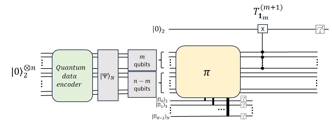
Figure 12: Quantum circuit implementation of randomization test

First recall that, any $n$-qubit state can be written as $\ket{\psi}_{N}=\sum_{j=0}^{N-1}x_{j}\ket{j}_{N},$ $N=2^{n}$ where $\{\ket{j}_{N}:0\leq j\leq N-1\}$ denotes the canonical computational basis for the $n$-qubit system. Then for a permutation gate $\pi\in\mathcal{S}_{N},$ we have

$$\pi\ket{\psi}_{N}=\sum_{j=0}^{N-1}x_{\pi(j)}\ket{j}_{N}.$$ (7)

It is needless to say that an $n$-qubit register carries a probability distribution. Besides, from equation (7) it follows that when a permutation $\pi$ acts on an $n$-qubit state, it preserves the probability distribution described by the quantum measurement wrt the canonical basis, since $\{|x_{j}|^{2}:0\leq j\leq N-1\}=\{|x_{\pi(j)}|^{2}:0\leq j\leq N-1\}.$

Algorithm 5 Quantum algorithm for two-sample randomization test

1:Create a distribution $p_{j},$ $0\leq j\leq 2^{n}-1$ where $p_{j}=a_{j}/(\sum_{j=0}^{2^{n}-1}a_{j})$ and implement it through a quantum data loader with an $n$-qubit quantum state

$$\ket{\Psi}_{N}=\sum_{j=0}^{2^{n}-1}\sqrt{p_{j}}\ket{j}_{N}.$$

2:Apply a random permutation $\pi$ on $\ket{\Psi}_{N}$ through the aforementioned procedure by performing simultaneous quantum measurements on the ancillary quantum states $\ket{\Pi_{l}}_{l+2},$ $0\leq l\leq N.$

3:Record the measurement outcome of ancillary quantum state $\ket{\Pi_{l}}_{l+2}$ for classical data analysis.

4:Then apply the $(m+1)$-qubit Toffoli gate $T_{\boldsymbol{1}_{m}}^{(m+1)}$ with control qubits as the first $m$ qubits of the $n$-qubit register and the target qubit as the ancillary qubit $\ket{0}_{2}$ (the first qubit of the entire $(n+1)$-qubit register, which we call the ‘First qubit’).

5:Perform a quantum measurement with respect to the Pauli $Z$ matrix on the First qubit, .

6:Record the outcome of the First qubit measurement.

7:Repeat the steps $2$ to $6$.

Analysis of the algorithm: One iteration of the algorithm would give us a pair of outcomes to keep in record for classical analysis of these outcomes for calculation of the means of the two samples of $K=2^{n-m}$ and $N-K=2^{n}-2^{n-m}$ data points. First observe that the permutation $\pi$ is obtained as $\prod_{s_{l}\in\Pi_{l}}s_{l},$ where each $s_{l}$ is observed after measuring $\ket{\Pi_{l}}_{l+2},$ $0\leq l\leq N-2$ wrt the computational basis measurement. Next, observe that the Toffoli gate $T_{\boldsymbol{1}_{m}}^{(m+1)}$ with control qubits as the first $m$ qubits of the $n$-qubit register is acted on the quantum state

$$\pi\ket{\Psi}_{N}\ket{0}_{2}=\sum_{j=0}^{2^{n}-1}\sqrt{p_{\pi(j)}}\ket{j}_{N}\ket{0}_{2}=\sum_{\begin{subarray}{c}j=(j_{n-1},\ldots,j_{0})\\ j_{l}\in\{0,1\}\end{subarray}}\sqrt{p_{\pi(\sum_{l=0}^{n-1}j_{l}2^{l})}}\ket{j_{n-1}j_{n-2}\ldots j_{0}}_{N}\ket{0}_{2}.$$

Then the output quantum state after applying the Toffoli gate is given by

$$T_{\boldsymbol{1}_{m}}^{(m+1)}\pi\ket{\Psi}_{N}\ket{0}_{2} = \sum_{\begin{subarray}{c}j_{l}\in\{0,1\}\\ (j_{m-1},\ldots,j_{0})={\bf 1}_{m}\end{subarray}}\sqrt{p_{\pi(\sum_{l=0}^{n-1}j_{l}2^{l})}}\ket{j_{n-1}j_{n-2}\ldots j_{0}}_{N}\ket{1}_{2}+$$ (8)

$$\sum_{\begin{subarray}{c}j_{l}\in\{0,1\}\\ (j_{m-1},\ldots,j_{0})\neq{\bf 1}_{m}\end{subarray}}\sqrt{p_{\pi(\sum_{l=0}^{n-1}j_{l}2^{l})}}\ket{j_{n-1}j_{n-2}\ldots j_{0}}_{N}\ket{0}_{2},$$

where ${\bf 1}_{m}$ is the all-one vector of dimension $m.$

It follows from the expression of the right-hand side of equation (8) that there are $K=2^{n-m}$ quatum states with First qubit state $\ket{1}_{2}$, and $N-K=2^{n}-2^{n-m}$ quantum states with First qubit state $\ket{0}_{2}.$ Obviously, the the probability that $\ket{1}_{2}$ or $\ket{0}_{2}$ is obtained after $Z$-axis measurement to the First qubit is given by

$$p=P\left(\mbox{First qubit}=\ket{1}_{2}\right) = \sum_{\begin{subarray}{c}j_{l}\in\{0,1\}\\ (j_{m-1},\ldots,j_{0})={\bf 1}_{m}\end{subarray}}p_{\pi(\sum_{l=0}^{n-1}j_{l}2^{l})}\,\,\mbox{and}$$

$$q=P\left(\mbox{First qubit}=\ket{0}_{2}\right) = 1-p=\sum_{\begin{subarray}{c}j_{l}\in\{0,1\}\\ (j_{m-1},\ldots,j_{0})\neq{\bf 1}_{m}\end{subarray}}p_{\pi(\sum_{l=0}^{n-1}j_{l}2^{l})},$$ (9)

respectively.

Now note that corresponding to the control qubits, which are the first $m$ qubits of the $n$-qubit register, for the Toffoli gate $T_{\boldsymbol{1}_{m}}^{(n)}$, the $K$ basis elements of the $n$-qubit system in the rhs of equation (8) are fixed whose corresponding coefficients determine $p$ and $q$ for any permutation $\pi$. These basis elements are given by $\ket{k},$ where

$$k=\sum_{j=0}^{m-1}2^{j}+\sum_{\begin{subarray}{c}l=m\\ j_{l}\in\{0,1\}\end{subarray}}^{n-1}j_{l}2^{j_{l}},$$ (10)

which we collect to denote the set $K$ for brevity. Each permutation assigns coefficients to these basis elements and there will be $K!\times(N-K)!$ permutations which will place the same set of coefficients in different permutations which will essentially be be used to compute $p$ and hence $q=1-p.$ While recording the permutation in each iteration, whether two different permutations, say $\pi$ and $\tau$ assign the same set of $K$ coefficients can be checked if and only if $\{\pi(j)|j\in K\}=\{\tau(j)|j\in K\}.$ Consequently, there are ${N\choose K}$ number of different sets of the coefficients which is equivalent to a partition of the permutation group $\mathcal{S}_{N}$ into ${N\choose K}$ classes, each of which contains $K!\times(N-K)!$ permutations.

Classical processing of the data obtained from the quantim circuit: Thus after generation of a random permutation $\pi$ through quantum circuits as a subroutine, it needs to be decided, which class it should belong to out of ${N\choose K}$ classes, which can be performed classically by determining the set $K_{\pi}=\{\pi(j):j\in K\},$ where $K$ is composed of all $k$ given by equation (10). The time complexity of obtaining the set $K_{\pi}$ for a $\pi$ is $O(1).$ Writing the set $K_{\pi}$ as an array $[K_{\pi}],$ the worst-case complexity of checking whether two arrays corresponding to two permutations $\pi,\tau$ obtained from the quantum random sampling method are identical is $O(K).$ Since there are ${N\choose K}$ sets of classes of permutations, and each randomly generated permutation belongs to one of these classes, upon quantum measurement of the First qubit, a classical register corresponding to each class will record the statistics of measurement outcomes either $0$ or $1$ according to the outcome $\ket{0}_{2}$ and $\ket{1}_{2}$ respectively. Thus the worst-case complexity up to this step is $O(K\cdot{N\choose K}).$ Now from the statistics of $0$ and $1$ in each class $C$ the probability value $p_{c}$ can be computed in $O(1)$ (which will be the same as described in equation (9)). It should be note that the value of $p_{c}$ is obtained from a collection of at least $K!\times(N-K)!$ $0$ and $1,$ when all the $N!$ permutations (at least once) are obtained through the quantum circuit generation.

Finally, for a given class $C$ of the set of permutations, we have

$$p_{c}=\sum_{k\in K}p_{k}=\sum_{k\in K}\frac{a_{k}^{c}}{\sum_{j=0}^{2^{n}-1}a_{j}}=\frac{\sum_{k\in K}a_{k}^{c}}{\sum_{j=0}^{2^{n}-1}a_{j}}=\mbox{Mean}\{a_{k}^{c}:k\in K\}\times\frac{K}{\sum_{j=0}^{2^{n}-1}a_{j}}$$ (11)

where $a_{k}^{c}$ is the set of data points belong to the class $C.$ Thus the mean of the sample data points corresponding to a class is obtained by multiplying $p$ with $\frac{\sum_{j=0}^{2^{n}-1}a_{j}}{K}.$ Thus the mean value for each sample can be estimated in $O(1)$ time from $p_{c}$. This concludes that the time complexity of processing the classical data obtained from the Algorithm 5 is given by $O(K\cdot{N\choose K}),$ which shows a $O(2^{m})$ improvement than the classical approach. For instance, if $m\approx n/2$ then $O(\sqrt{2^{n}})$ improvement can be observed.

The advantage of the proposed quantum algorithm is that, the mean values of the two samples for a class $C$ of permutations can be obtained from estimation of the probability values $p_{c}$ and $q_{c}=1-p_{c},$ which are obtained by measurement of the ancillary First qubit for each random sampling of permutations. Finally, the $p$-value of the test can be calculated using these probability values to test the null hypothesis.

We have the following remarks about the proposed algorithm.

Remark 4.1.

1. The choice of the $m$ control qubits to apply the Toffoli gate can be chosen as any of the $m$ qubits from the $n$ qubits. Here we choose the first $m$ qubits.

2. Note that the algorithm need not be continued till all permutations are generated through the random sampling of permutation generation using the quantum circuit. When $N$ is large, the number $K!\times(N-K)!$ is also a large number, and we do not need that many measurements to estimate the $p_{c}$ value for a class. Instead, a minimal number can be decided for the number of observations for each class to estimate $p_{c}$, and when it is reached the entire process can be stopped for classical processing of the data.

5 Random sampling from a specific set of permutations

It is well known that a certain set of permutations is needed to perform various permutation tests [31]. In this section, we propose a quantum measurement based procedure for sampling permutations from a desired set of permutations, which is decided by the choice of the ancillary quantum states for simultaneous measurement. We give a combinatorial perspective of the sampling method by introducing a nested corona product representation of symmetric groups.

5.1 Nested corona product graph representation of symmetric groups

First we recall the definition of corona product of graphs, which was introduced in the context of wreath product of the groups, in particular, symmetric groups [32].

Definition 5.1.

(Corona product of two graphs) Let $G$ and $H$ be two graphs on $n$ and $k$ vertices respectively. Then the corona of $G$ and $H,$ denoted by $G\circ H$ is formed by taking one copy of $G$ and $n$ copies of $H$ such that $i$-th vertex of $G$ is joined by an edge of every vertex of the $i$-th copy of $H.$

Following Definition 5.1, if $V(G)$ and $V(H)$ denote the vertex sets of $G$ and $H$ respectively, then $G\circ H$ has $|V(G)|+(|V(G)|\times|V(H)|)$ number of vertices, whereas number of edges of $G\circ H$ is $|E(G)|+(|V(G)|\times|V(H)|)+(|V(G)|\times|E(G)|)=|E(G)|+|V(G)|(|V(H)|+|E(G)|),$ where $E(X)$ denotes number of edges of the graph $X.$ Further, given a graph $G$ on $n$ vertices, and a collection of graphs $H_{1},\ldots,H_{n},$ the generalized corona graph, denoted by $G\circ\wedge_{i=1}^{n}H_{i}$ is defined as taking one copies of $G,$ $H_{1},\ldots,H_{n}$ join the $i$-th vertex of $G$ to all the vertices of $H_{i}$ by an edge [33]. Further, given a graph $G^{(0)},$ the corona graphs are introduced in [34] for the proposal of a large graph generative model by taking the corona product of $G^{(0)}$ iteratively. Indeed, for a given positive integer $m\geq 1,$ the corona graph $G^{(m)}$ is defined as $G^{(m)}=G^{(m-1)}\circ G^{(0)}.$

In what follows, we introduce nested corona product for an ordered set of simple graphs $\{G_{0},G_{1},\ldots,G_{N-2}\}.$ By simple graph, we mean a graph with no loops and only one edge can exist between two vertices.

Definition 5.2.

(Nested corona product of an ordered set of graphs) Let $\{G_{0},G_{1},\ldots,G_{N-2}\}$ be an ordered set of simple graphs. Then the nested corona product graph is defined as

$$\circledwedge_{j=0}^{N-2}G_{j}:=(\cdots((G_{0}\circ G_{1})\circ G_{2})\cdots)\circ G_{N-2}.$$

Let $G^{\circledwedge N-1}:=\circledwedge_{j=0}^{N-2}G_{j},$ $N\geq 3$ with $|V(G_{j})|=n_{j}$ and $|E(G_{j})|=m_{j}.$ Then there is a recurrence relation for the number of vertices for the nested corona product graphs given by

$$\left|V\left(G^{\circledwedge k}\right)\right|=\left|V\left(G^{\circledwedge k-1}\right)\right|+\left(\left|V\left(G^{\circledwedge k-1}\right)\right|\times\left|V\left(G_{k-1}\right)\right|\right),k\geq 2.$$ (12)

Before proceeding to derive the number of vertices and edges in a nested corona product graph, we recall the following from [35].

The elementary symmetric polynomials for a given set of $n$ variables $x_{1},\ldots,x_{n}$ are given by

1. $e_{0}(x_{1},\ldots,x_{n})=1$ (by convention)

2. $e_{1}(x_{1},\ldots,x_{n})=\sum_{j=1}x_{j}$

3. $e_{2}(x_{1},\ldots,x_{n})=\sum_{1\leq i<j\leq n}x_{i}x_{j}$

4. $\vdots$

5. $e_{n}(x_{1},\ldots,x_{n})=x_{1}x_{2}\cdots x_{n}.$

Further,

$$\sum_{k=0}^{n}e_{k}(x_{1},\ldots,x_{n})=(1+x_{1})(1+x_{2})\cdots(1+x_{n}).$$ (13)

Theorem 5.3.

$G^{\circledwedge N-1}:=\circledwedge_{j=0}^{N-2}G_{j},$ $N\geq 3$ with $|V(G_{j})|=n_{j}$ and $|E(G_{j})|=m_{j}.$ Then

$$\left|V(G^{\circledwedge N-1})\right| = n_{0}(1+n_{1})(1+n_{2})\cdots(1+n_{N-2}),$$

$$\left|E(G^{\circledwedge N-1})\right| = m_{0}+\sum_{j=0}^{N-3}(n_{0}+\ldots+n_{j})(n_{j+1}+m_{j+1}).$$

Proof: The proof for $\left|V(G^{\circledwedge N-1})\right|$ follows from repeated application of the recurrence relation given by equation (12). Indeed, from the definition of nested corona product graph, it follows that

$$\left|V(G^{\circledwedge N-1})\right|=n_{0}\left(1+\sum_{l=1}^{N-2}n_{l}+\sum_{\begin{subarray}{c}l_{1}\neq l_{2}\\ l_{1},l_{2}=1\end{subarray}}^{N-2}n_{l_{1}}n_{l_{2}}+\sum_{\begin{subarray}{c}l_{1}\neq l_{2}\neq l_{3}\\ l_{1},l_{2},l_{3}=1\end{subarray}}^{N-2}n_{l_{1}}n_{l_{2}}n_{l_{3}}+\ldots+\sum_{\begin{subarray}{c}l_{1}\neq l_{2}\neq l_{3},\ldots,\neq l_{N-3}\\ l_{1},l_{2},l_{3},\ldots,l_{N-3}=1\end{subarray}}^{N-2}n_{l_{1}}n_{l_{2}}n_{l_{3}}\cdots n_{l_{N-3}}+\prod_{l=1}^{N-2}n_{l}\right).$$

Then note that each term of the sum is a symmetric polynomial for $N-2$ variables, which are the number of vertices $n_{1},\ldots,n_{N-2}.$ Then the result follows from equation (13).

For the number of edges, the proof follows from the formation of the nested corona product graph, which is given by

$$\left|E(G^{\circledwedge N-1})\right|=m_{0}+n_{0}(n_{1}+m_{1})+(n_{0}+n_{1})(n_{2}+m_{2})+\ldots+(n_{0}+\ldots+n_{N-3})(n_{k-1}+m_{N-2}).$$

This completes the proof. $\square$

Now we derive certain characteristics of $G^{\circledwedge N-1},$ $N\geq 3$ that will be used in sequel. First, observe that the number of copies of a $G_{j},$ $2\leq j\leq N-2$ that gets attached during the formation of $G^{\circledwedge N-1}$ is given by $\left|V(G^{\circledwedge j})\right|=n_{0}(1+n_{1})(1+n_{2})\ldots(1+n_{j-1}),$ where $G^{\circledwedge j}=(\cdots((G_{0}\circ G_{1})\circ G_{2})\circ\cdots G_{j-1}).$ Obviously, number of copies of $G_{1}$ that gets attached is $n_{0}=|V(G_{0})|.$ We denote the $i$-th copy of $G_{j}$ as $G_{j}^{(i)}$ with the vertex set $\{v^{j}_{i,1},\ldots,v^{j}_{i,n_{j}}\},$ $1\leq i\leq n_{0}(1+n_{1})\cdots(1+n_{j-1}).$ Besides, denote the vertices of $G_{0}$ in $G^{\circledwedge N-1}$ as $\{v^{0}_{0,1},\cdots,v^{0}_{0,n_{0}}\},$ and the vertices of $i$-th copy of $G_{1}$ is given by $\{v^{1}_{i,1},\ldots,v^{1}_{i,n_{1}}\}$ for $1\leq i\leq n_{0}.$ Finally, the vertex set of $G^{\circledwedge N-1}$ is given by

$$V^{\circledwedge N-1} = \left\{v^{0}_{0,1},\cdots,v^{0}_{0,n_{0}}\right\}\bigcup\left\{v^{1}_{i,l}:1\leq i\leq n_{0},1\leq l\leq n_{1}\right\}\bigcup$$ (14)

$$\left\{v^{j}_{i,1},\cdots,v^{j}_{i,n_{j}}:2\leq j\leq N-2,1\leq i\leq n_{0}(1+n_{1})\cdots(1+n_{j-1})\right\}.$$

Now let $d^{(j)}_{1},\ldots,d^{(j)}_{n_{j}}$ denote the degree of the vertices $v^{(j)}_{i,1},\ldots,v^{(j)}_{i,n_{j}}$ of the $i$-th copy of the graph $G_{j},$ respectively, $0\leq j\leq N-2.$ Then the degree of a vertex $v^{(j)}_{i,s}$ after formation of the nested corona product graph is given by $1+d_{s}^{(j)}+\sum_{l=j+1}^{N-2}n_{l},$ $1\leq s\leq n_{j}$, where $1$ appears due to the attachment of $G_{j}^{(i)}$ to an existing vertex of the graph $G^{\circledwedge j}$, and the term $\sum_{l=j+1}^{N-2}n_{l}$ appears due to the definition of nested corona product graph $G^{\circledwedge N-1}.$

Now, we consider a path graph representation of $\Pi_{0}=\{I,s_{0}\}$ and $\overline{\Pi}_{k}=\Pi_{k}\setminus\{I\}=\{s_{k},s_{k}s_{k-1},\ldots,s_{k}s_{k-1}\cdots s_{0}\},$ $1\leq k\leq N-2,$ where $\Pi_{0}^{G}$ represents path (an edge) with two vertices labelled as $I$ and $s_{0},$ whereas $\overline{\Pi}_{k}^{G}$ denotes the path graph on $k+1$ vertices labelled as $s_{k}=v^{(k)}_{1},s_{k}s_{k-1}=v^{(k)}_{2},\ldots,s_{k}s_{k-1}\cdots s_{0}=v^{(k)}_{k+1}$ with edges between $v^{(k)}_{l}$ and $v^{(k)}_{l+1},$ $1\leq l\leq k.$ See Figure LABEL:Fig:gforsym for $\overline{\Pi}^{G}_{k},$ $k=1,2,$ and $\Pi^{G}_{0}.$ Now we propose a nested corona product graph representation of the symmetric group.

Indeed, the number of vertices of $\circledwedge_{j=0}^{N-2}G_{j},\,G_{0}=\Pi_{0},G_{j}=\overline{\Pi}_{j},j\geq 1$ is $N!$ as described by the following corollary.

Corollary 5.4.

Let $G=\circledwedge_{j=0}^{N-2}G_{j},\,G_{0}=\Pi_{0}^{G},G_{j}=\overline{\Pi}_{j}^{G},j\geq 1.$ Then $\left|V(G)\right|=N!.$

Proof: Setting $n_{0}=2$, $n_{1}=2$ and $n_{l}=l+1$ for $l\geq 3$ the desired result follows from Theorem 5.3. Indeed

$$n_{0}(1+n_{1})(1+n_{2})+\cdots+(1+n_{N-2})=2(1+2)(1+3)\cdots(1+N-1)=2\cdot 3\cdot 4\cdots N=N!.$$

This completes the proof. $\square$

Now we describe the graph $G$ defined in Corollary 5.4 as the graph representation of the symmetric group $\mathcal{S}_{k}$ by assigning the labelling of the vertices as permutations as per the following procedure.

Algorithm 6 Nested corona product graph generative model $\mathcal{S}_{N}^{G}$ for symmetric group on $N\geq 3$ elements

1:The graph representation of $\mathcal{S}_{2}$ is $\Pi_{0}^{G},$ denoted as $\mathcal{S}^{G}_{2}.$

2:Label the vertices of $\overline{\Pi}_{k}^{G},$ $k\geq 1$ as the permutations $s_{k},s_{k}s_{k-1},\ldots,s_{k}s_{k-1}\cdots s_{0}.$

3:When a copy of $\overline{\Pi}_{k}^{G}$ is attached to an existing vertex labelled with a permutation $\pi$ in the nested corona product graph then the labelling of the vertices of that $\overline{\Pi}_{k}^{G}$ are assigned as $\pi s_{k},$ $\pi s_{k}s_{k-1},$ $\ldots,$ $\pi s_{k}s_{k-1}\cdots s_{0}.$

4:For $N\geq 3,$

$$\mathcal{S}_{N}^{G}=\circledwedge_{j=0}^{N-2}G_{j},\,G_{0}=\Pi_{0}^{G},G_{j}=\overline{\Pi}_{j}^{G},j\geq 1.$$

In Figure LABEL:Fig:gforsym we provide the nested corona product graph representation of the symmetric groups $\mathcal{S}_{k}$ for $k=2,3,4.$

Remark 5.5.

It should be noted that the choice of representing the set of permutations $\Pi_{0}$ and $\overline{\Pi}_{k},$ $k\geq 1$ by path graphs is ad-hoc, and indeed it can be represented by any (simple) graph on $|\Pi_{0}|$ and $|\overline{\Pi}_{k}|$ vertices, such as star graph, complete graph or even the null graph with no edges. We justify our choice of the graphs $\Pi_{0}^{G}$ and $\overline{\Pi}_{k}^{G},$ $k\geq 1$ as follows:

1. If the graph representing $\Pi_{0}=\{I,s_{0}\}$ is disconnected then the graph $S^{G}_{k}$ would be disconnected for all $k,$ hence the only option to consider an edge graph for $\Pi_{0}$ so that the resulting graphs remain connected.

2. The least number of a edges in a connected graph on a set of vertices is the path graph, so the choice of path graph for $\overline{\Pi}_{k}$, $k\geq 1$ does not explode with a large number of edges in $S^{G}_{N}.$ Secondly, since the vertices are represented by permutations in $\overline{\Pi}_{k},$ the choice of path graph has an algebraic interpretation: any two vertices $\pi$ and $\tau$ are linked by an edge if and only if $\pi=s\tau$ for some adjacent transposition $s.$

Obviously, it follows from the Corollary 5.4 and Algorithm 6 that the number of vertices of $\mathcal{S}_{N}^{G}$ is $N!,$ which equals the number of permutations on $N$ elements. An interesting property of $S^{G}_{N}$ is that it is union of two the two isomorphic subgraphs, one originated at $I$ and the other originated at $s_{0}$, which are joined by the edge $(I,s_{0}).$

5.2 Quantum circuit methods for sampling permutations from $\mathcal{S}_{N}^{G}$

In this section, we show that the circuit model of random sampling of permutations for $n$-qubit systems as discussed in Section 4 and the nested corona product graph representation of symmetric groups enable us to sample permutations from specific sets of permutations. Note that permutations on $n$-qubit systems are vertices of the graph $S_{2^{n}}^{G}.$ Thus in this section, we set $N=2^{n}.$

From equation (14) and Algorithm 6 it follows that each vertex of $S_{N}^{G}$ represents a permutation and any such permutation is decided by a copy of $\overline{\Pi}_{j}^{G},$ $1\leq j\leq N-2$ which gets attached to an existing vertex. On the other hand, modifying the quantum circuit given by Figure 11 with each ancillary quantum state $\ket{\Pi_{k}}_{k+2},$ $k\geq 1$ replaced by $\ket{\overline{\Pi}_{k}}_{k+1}=\sum_{j=0}^{k}\frac{1}{\sqrt{k+1}}\ket{j}_{k+1}$ defined as follows, drives a technique for efficient sampling of permutations.

Figure 20: Quantum circuit for sampling of specific permutations

Below we list how to perform random sampling of permutations through the quantum circuit given by Figure 20 from some specific subsets of vertices of $\mathcal{S}_{N}^{G}.$

1. Sampling from $\Pi_{0}$ and $\overline{\Pi}_{k},$ $k\geq 1:$ Note that sampling from $\Pi_{0}$ can be done by measuring $\ket{\Pi_{0}}_{2}.$ Note that the permutations in $\overline{\Pi}_{k}$ for any $k\geq 1$ are represented by the vertices when a copy of $\overline{\Pi}_{k}^{G}$ is attached to the vertex $I$ of $\Pi_{0}^{G}.$ Thus sampling from nontrivial permutations in $\Pi_{k}$ can be done by performing a measurement to the state $\ket{\overline{\Pi}_{k}}.$

2. Sampling from $\overline{\Pi}_{l}\overline{\Pi}_{m}=\{\pi\tau:\pi\in\overline{\Pi}_{k},\tau\in\overline{\Pi}_{l}\}$, $l<m\leq N-2$: The permutations in $\overline{\Pi}_{l}\overline{\Pi}_{m}$ are represented by the vertices which are the vertices of all the copies of $\overline{\Pi}_{m}$ when each of which gets attached to all the vertices of a copy of $\overline{\Pi}^{G}_{l}$, which is attached to $I$ (a vertex in $\Pi_{0}^{G}$) during the formation of $S^{G}_{k}.$ Thus making make a simultaneous measurement of both $\ket{\overline{\Pi}_{l}}_{l+1}$ and $\ket{\overline{\Pi}_{m}}_{m+1}$ gives the desired result.

3. Sampling from the set of permutations which are represented by vertices in a copy of $\overline{\Pi}_{j}^{G}$ for some $1\leq j\leq N-2$ in $\mathcal{S}_{N}^{G}:$ The permutations corresponding to the vertices of a copy of $\overline{\Pi}_{j}^{G}$ are of the form $\pi\tau,$ where $\tau\in\overline{\Pi}_{j}=\{s_{j},s_{j}s_{j-1},\ldots,s_{j}s_{j-1}\cdots s_{0}\}$ and $\pi$ is the permutation corresponding to the vertex to which $\overline{\Pi}_{j}^{G}$ is attached due to the definition of $\mathcal{S}_{N}^{G}.$ Now observe that $\pi$ is a vertex of $\overline{\Pi}_{l}^{G}$ for some $l<j,$ and it continues to obtain $\pi=\pi_{1}\pi_{2}\cdots\pi_{m}$ such that $\pi_{i}\in V(\Pi^{G}_{k_{i}})$ for some $k_{1}<k_{2}<\ldots<k_{m}<j$ with $\pi_{1}\in\{I,s_{0}\}=V(\Pi_{0}^{G}).$ Besides, if the vertex corresponding to $\pi_{k_{i}}$ in $\overline{\Pi}_{k_{i}}^{G}$ represents the $l_{i}$-th element of $\overline{\Pi}_{k}^{G}$ then setting the states $\ket{\overline{\Pi}_{k_{i}}}_{k_{i}+1}$ as $\ket{l_{i}}_{k_{i}+1}$ in the quantum circuit (Figure 20) for $i=1,2,\ldots,m$, the measurement of $\ket{\overline{\Pi}_{j}}_{j+1}$ will generate a sample from the desired set of permutations. Obviously, any permutation from the desired set will be sampled with probability $\frac{1}{j+1}.$

   The equivalent combinatorial interpretation of this method is to identify the shortest path from the vertex $I$ or $s_{0}$ to the set of vertices chosen for sampling the permutations from.

From the above procedures, it is clear that the graph theoretic interpretation of sampling a set of $k+1,$ $1\leq k\leq N-2$ permutations represented by the set of vertices $\{v^{j}_{i,1},v^{j}_{i,2},\ldots,v^{j}_{i,n_{j}}\},$ as discussed in equation (14) (here $n_{j}=j+1$ since $G_{j}=\overline{\Pi}_{j}^{G}$) is the identification of the shortest path either from $I$ or $s_{0},$ the vertices of $\Pi_{0}^{G}$ to the vertex to which the copy of $G_{j}$ is attached due to the formation of the corona product. Identification of the intermediate vertices of the graphs $\overline{\Pi}_{k}^{G},$ $k<j$ graphs would essentially decide the ancillary states $\ket{\overline{\Pi}_{k}}_{k+1}$ for executing the circuit simulation for the sampling.

Conclusion. In this paper, we proposed new classical algorithms for random sampling of permutations on $k\geq 2$ elements by finding a way to express them as products of at most $k(k-1)/2$ adjacent transpositions. This algorithm is further implemented in a quantum circuit model for permutations on $n$-qubit systems. This is achieved by constructing quantum circuit representations of adjacent permutations using $X$ gate, CNOT gate, and standard $n$-qubit Toffoli gate. Thus a quantum circuit model with $N-1$ ancillary qudit states $2\leq d\leq 2^{n}$ is developed for random sampling from the symmetric groups $\mathcal{S}_{2^{n}},$ $n\geq 1$ through quantum measurement of these qudits. Next, this circuit is applied to develop a quantum algorithm for the two-sample randomization test. Finally, a nested corona product graph generative model is defined to provide graph representation of symmetric groups, which is further used to define a quantum circuit model for random sampling from specific sets of permutations of $2^{n}$ elements.

This work gives rise to several open problems, two of which are listed below.

1. The product of adjacent transpositions that belong to a $\Pi_{k}$ can be represented by alternative circuits which may not need use of any Toffoli gate but a collection of CNOT gates, since any CNOT gate $X_{ij}$ represents a permutation matrix on $n$-qubit systems. Thus minimization of number of quantum gates to define the quantum circuit model for random sampling circuit is a potential problem that can be investigated to reduce the number of gates in use.

2. Considering the symmetric group as a Coxeter group, it is fascinating to systematically obtain the elements of the group as products of its generators, specifically adjacent transpositions, derived from the corresponding Coxeter graph. This combinatorial approach prompts the question: can this method be extended to other Coxeter groups?

6 Appendix

N	Permutations	Decomposition
2	$[0,{\color[rgb]{1,0,0}1}]_{1}=\left(\begin{matrix}0&1\\ 0&1\end{matrix}\right)$	$I$
	$[{\color[rgb]{1,0,0}1},0]_{1}=\left(\begin{matrix}0&1\\ 1&0\end{matrix}\right)=(0,1)$	$s_{0}$
3	$[0,1,{\color[rgb]{1,0,0}2}]_{1}=\left(\begin{matrix}0&1&2\\ 0&1&2\end{matrix}\right)$	$I$
	$[0,{\color[rgb]{1,0,0}2},1]_{1}=\left(\begin{matrix}0&1&2\\ 0&2&1\end{matrix}\right)=(1,2)$	$Is_{1}=s_{1}$
	$[{\color[rgb]{1,0,0}2},0,1]_{1}=\left(\begin{matrix}0&1&2\\ 2&0&1\end{matrix}\right)=(0,2,1)$	$Is_{1}s_{0}=s_{1}s_{0}$
	$[1,0,{\color[rgb]{1,0,0}2}]_{2}=\left(\begin{matrix}0&1&2\\ 1&0&2\end{matrix}\right)=(0,1)$	$s_{0}$
	$[1,{\color[rgb]{1,0,0}2},0]_{2}=\left(\begin{matrix}0&1&2\\ 1&2&0\end{matrix}\right)=(0,1,2)$	$s_{0}s_{1}$
	$[{\color[rgb]{1,0,0}2},1,0]_{2}=\left(\begin{matrix}0&1&2\\ 2&1&0\end{matrix}\right)=(0,2)$	$s_{0}s_{1}s_{0}$

Table 1: Writing permutations in $\mathcal{S}_{k},$ $k=2,3$ obtained from Steinhaus-Johnson-Trotter algorithm as product of adjacent transpositions

N	Permutations	Decomposition
4	$[0,1,2,{\color[rgb]{1,0,0}3}]_{1}=\left(\begin{matrix}0&1&2&3\\ 0&1&2&3\end{matrix}\right)$	$I$
	$[0,1,2,{\color[rgb]{1,0,0}3}]_{1}=\left(\begin{matrix}0&1&2&3\\ 0&1&2&3\end{matrix}\right)=(2,3)$	$Is_{2}=s_{2}$
	$[0,{\color[rgb]{1,0,0}3},1,2]_{1}=\left(\begin{matrix}0&1&2&3\\ 0&3&1&2\end{matrix}\right)=(1,3,2)$	$Is_{2}s_{1}=s_{2}s_{1}$
	$[{\color[rgb]{1,0,0}3},0,1,2]_{1}=\left(\begin{matrix}0&1&2&3\\ 3&0&1&2\end{matrix}\right)=(0,3,2,1)$	$Is_{2}s_{1}s_{0}=s_{2}s_{1}s_{0}$
	$[0,2,1,{\color[rgb]{1,0,0}3}]_{2}=\left(\begin{matrix}0&1&2&3\\ 0&2&1&3\end{matrix}\right)=(1,2)$	$s_{1}$
	$[0,2,{\color[rgb]{1,0,0}3},1]_{2}=\left(\begin{matrix}0&1&2&3\\ 0&2&3&1\end{matrix}\right)=(1,2,3)$	$s_{1}s_{2}$
	$[0,{\color[rgb]{1,0,0}3},2,1]_{2}=\left(\begin{matrix}0&1&2&3\\ 0&3&2&1\end{matrix}\right)=(1,3)$	$s_{1}s_{2}s_{1}$
	$[{\color[rgb]{1,0,0}3},0,2,1]_{2}=\left(\begin{matrix}0&1&2&3\\ 3&0&2&1\end{matrix}\right)=(0,3,1)$	$s_{1}s_{2}s_{1}s_{0}$
	$[2,0,1,{\color[rgb]{1,0,0}3}]_{3}=\left(\begin{matrix}0&1&2&3\\ 2&0&1&3\end{matrix}\right)=(0,2,1)$	$s_{1}s_{0}$
	$[2,0,{\color[rgb]{1,0,0}3},1]_{3}=\left(\begin{matrix}0&1&2&3\\ 2&0&3&1\end{matrix}\right)=(0,2,3,1)$	$s_{1}s_{0}s_{2}$
	$[2,{\color[rgb]{1,0,0}3},0,1]_{3}=\left(\begin{matrix}0&1&2&3\\ 2&3&0&1\end{matrix}\right)=(0,2)(1,3)$	$s_{1}s_{0}s_{2}s_{1}$
	$[{\color[rgb]{1,0,0}3},2,0,1]_{3}=\left(\begin{matrix}0&1&2&3\\ 3&2&0&1\end{matrix}\right)=(0,3,1,2)$	$s_{1}s_{0}s_{2}s_{1}s_{0}$
	$[1,0,2,{\color[rgb]{1,0,0}3}]_{4}=\left(\begin{matrix}0&1&2&3\\ 1&0&2&3\end{matrix}\right)=(0,1)$	$s_{0}$
	$[1,0,{\color[rgb]{1,0,0}3},2]_{4}=\left(\begin{matrix}0&1&2&3\\ 1&0&3&2\end{matrix}\right)=(0,1)(2,3)$	$s_{0}s_{2}$
	$[1,{\color[rgb]{1,0,0}3},0,2]_{4}=\left(\begin{matrix}0&1&2&3\\ 1&3&0&2\end{matrix}\right)=(0,1,3,2)$	$s_{0}s_{2}s_{1}$
	$[{\color[rgb]{1,0,0}3},1,0,2]_{4}=\left(\begin{matrix}0&1&2&3\\ 3&1&0&2\end{matrix}\right)=(0,3,2)$	$s_{0}s_{2}s_{1}s_{0}$
	$[1,2,0,{\color[rgb]{1,0,0}3}]_{5}=\left(\begin{matrix}0&1&2&3\\ 1&2&0&3\end{matrix}\right)=(0,1,2)$	$s_{0}s_{1}$
	$[1,2,{\color[rgb]{1,0,0}3},0]_{5}=\left(\begin{matrix}0&1&2&3\\ 1&2&3&0\end{matrix}\right)=(0,1,2,3)$	$s_{0}s_{1}s_{2}$
	$[1,{\color[rgb]{1,0,0}3},2,0]_{5}=\left(\begin{matrix}0&1&2&3\\ 1&3&2&0\end{matrix}\right)=(0,1,3)$	$s_{0}s_{1}s_{2}s_{1}$
	$[{\color[rgb]{1,0,0}3},1,2,0]_{5}=\left(\begin{matrix}0&1&2&3\\ 3&1&2&0\end{matrix}\right)=(0,3)$	$s_{0}s_{1}s_{2}s_{1}s_{0}$
	$[2,1,0,{\color[rgb]{1,0,0}3}]_{6}=\left(\begin{matrix}0&1&2&3\\ 2&1&0&3\end{matrix}\right)=(0,2)$	$s_{0}s_{1}s_{0}$
	$[2,1,{\color[rgb]{1,0,0}3},0]_{6}=\left(\begin{matrix}0&1&2&3\\ 2&1&3&0\end{matrix}\right)=(0,2,3)$	$s_{0}s_{1}s_{0}s_{2}$
	$[2,{\color[rgb]{1,0,0}3},1,0]_{6}=\left(\begin{matrix}0&1&2&3\\ 2&3&1&0\end{matrix}\right)=(0,2,1,3)$	$s_{0}s_{1}s_{0}s_{2}s_{1}$
	$[{\color[rgb]{1,0,0}3},2,1,0]_{6}=\left(\begin{matrix}0&1&2&3\\ 3&2&1&0\end{matrix}\right)=(0,3)(1,2)$	$s_{0}s_{1}s_{0}s_{2}s_{1}s_{0}$

Table 2: Writing permutations in $\mathcal{S}_{4}$ obtained from Steinhaus-Johnson-Trotter algorithm as product of adjacent transpositions

References

• [1] Robert Sedgewick. Permutation generation methods. ACM Computing Surveys (CSUR), 9(2):137โ€“164, 1977.
• [2] Donaldย E Knuth. The art of computer programming, volume 4A: combinatorial algorithms, part 1. Pearson Education India, 2011.
• [3] Alessandro Budroni, Isaacย A Canales-Martรญnez, and Lucasย Pandolfo Perin. Sok: Methods for sampling random permutations in post-quantum cryptography. Cryptology ePrint Archive, 2024.
• [4] Randy Kuang and Michel Barbeau. Quantum permutation pad for universal quantum-safe cryptography. Quantum Information Processing, 21(6):211, 2022.
• [5] Jamie Heredge, Charles Hill, Lloyd Hollenberg, and Martin Sevior. Permutation invariant encodings for quantum machine learning with point cloud data. Quantum Machine Intelligence, 6(1):1โ€“14, 2024.
• [6] Tobias Moroder, Philipp Hyllus, Gรฉza Tรณth, Christian Schwemmer, Alexander Niggebaum, Stefanie Gaile, Otfried Gรผhne, and Harald Weinfurter. Permutationally invariant state reconstruction. New Journal of Physics, 14(10):105001, 2012.
• [7] Gรฉza Tรณth and Otfried Gรผhne. Entanglement and permutational symmetry. Physical review letters, 102(17):170503, 2009.
• [8] Amir Fijany and Colinย P Williams. Quantum wavelet transforms: Fast algorithms and complete circuits. In Quantum Computing and Quantum Communications: First NASA International Conference, QCQCโ€™98 Palm Springs, California, USA February 17โ€“20, 1998 Selected Papers, pages 10โ€“33. Springer, 1999.
• [9] Mehdi Saeedi and Igorย L Markov. Synthesis and optimization of reversible circuitsโ€”a survey. ACM Computing Surveys (CSUR), 45(2):1โ€“34, 2013.
• [10] Sebastian Egner, Markus Pรผschel, and Thomas Beth. Decomposing a permutation into a conjugated tensor product. In Proceedings of the 1997 international symposium on Symbolic and algebraic computation, pages 101โ€“108, 1997.
• [11] Vivekย V Shende, Adityaย K Prasad, Igorย L Markov, and Johnย P Hayes. Synthesis of reversible logic circuits. IEEE Transactions on Computer-Aided Design of Integrated Circuits and Systems, 22(6):710โ€“722, 2003.
• [12] Mathias Soeken, Fereshte Mozafari, Bruno Schmitt, and Giovanni Deย Micheli. Compiling permutations for superconducting qpus. In 2019 Design, Automation & Test in Europe Conference & Exhibition (DATE), pages 1349โ€“1354. IEEE, 2019.
• [13] Cynthia Chen, Bruno Schmitt, Helena Zhang, Levย S Bishop, and Ali Javadi-Abhar. Optimizing quantum circuit synthesis for permutations using recursion. In Proceedings of the 59th ACM/IEEE Design Automation Conference, pages 7โ€“12, 2022.
• [14] Marc Bataille. Quantum circuits of cnot gates: optimization and entanglement. Quantum Information Processing, 21(7):269, 2022.
• [15] Rohitย Sarma Sarkar and Bibhas Adhikari. A quantum neural network framework for scalable quantum circuit approximation of unitary matrices. arXiv preprint arXiv:2405.00012, 2024.
• [16] Anders Bjรถrner and Francesco Brenti. Combinatorics of Coxeter groups, volume 231. Springer, 2005.
• [17] Phillip Good. Permutation tests: a practical guide to resampling methods for testing hypotheses. Springer Science & Business Media, 2013.
• [18] Michaelย D Ernst. Permutation methods: a basis for exact inference. Statistical Science, pages 676โ€“685, 2004.
• [19] Joe Sawada and Aaron Williams. Solving the sigma-tau problem. ACM Transactions on Algorithms (TALG), 16(1):1โ€“17, 2019.
• [20] Markย B Wells. Generation of permutations by transposition. Mathematics of Computation, 15(74):192โ€“195, 1961.
• [21] Haleย F Trotter. Algorithm 115: perm. Communications of the ACM, 5(8):434โ€“435, 1962.
• [22] Selmerย M Johnson. Generation of permutations by adjacent transposition. Mathematics of computation, 17(83):282โ€“285, 1963.
• [23] Hugo Steinhaus. One hundred problems in elementary mathematics. Courier Corporation, 1979.
• [24] Jean Cardinal, Hungย P Hoang, Arturo Merino, Ondล™ej Miฤka, and Torsten Mรผtze. Combinatorial generation via permutation languages. v. acyclic orientations. SIAM Journal on Discrete Mathematics, 37(3):1509โ€“1547, 2023.
• [25] Guy deย Balbine. Note on random permutations. Mathematics of Computation, 21(100):710โ€“712, 1967.
• [26] Wendy Myrvold and Frank Ruskey. Ranking and unranking permutations in linear time. Information Processing Letters, 79(6):281โ€“284, 2001.
• [27] Bibhas Adhikari and Aryan Jha. Local hamiltonian decomposition and classical simulation of parametrized quantum circuits. arXiv preprint arXiv:2401.13156, 2024.
• [28] Ronaldย Aylmer Fisher. The comparison of samples with possibly unequal variances. Annals of Eugenics, 9(2):174โ€“180, 1939.
• [29] Erichย Leo Lehmann and Howardย JM Dโ€™Abrera. Nonparametrics: statistical methods based on ranks, volume 464. Springer New York, 2006.
• [30] Jamesย J Higgins. An introduction to modern nonparametric statistics. Brooks/Cole Pacific Grove, CA, 2004.
• [31] Aaditya Ramdas, Rinaย Foygel Barber, Emmanuelย J Candรจs, and Ryanย J Tibshirani. Permutation tests using arbitrary permutation distributions. Sankhya A, 85(2):1156โ€“1177, 2023.
• [32] Roberto Frucht and Frank Harary. On the corona of two graphs. 1970.
• [33] ARย Fiuj Laali, Hย Hajย Seyyed Javadi, and Dariush Kiani. Spectra of generalized corona of graphs. Linear Algebra and its Applications, 493:411โ€“425, 2016.
• [34] Rohan Sharma, Bibhas Adhikari, and Abhishek Mishra. Structural and spectral properties of corona graphs. Discrete Applied Mathematics, 228:14โ€“31, 2017.
• [35] David Cox, John Little, Donal Oโ€™shea, and Moss Sweedler. Ideals, varieties, and algorithms, volumeย 3. Springer, 1997.