Geometry of the cumulant series in neuroimaging

Abstract

Water diffusion gives rise to micrometer-scale sensitivity of diffusion MRI (dMRI) to cellular-level tissue structure. The advent of precision medicine and quantitative imaging hinges on revealing the information content of dMRI, and providing its parsimonious basis- and hardware-independent “fingerprint”. Here we reveal the geometry of a multi-dimensional dMRI signal, classify all 21 invariants of diffusion and covariance tensors in terms of irreducible representations of the group of rotations, and relate them to tissue properties. Previously studied dMRI contrasts are expressed via 7 invariants, while the remaining 14 provide novel complementary information. We design acquisitions based on icosahedral vertices guaranteeing minimal number of measurements to determine 3–4 most used invariants in only 1–2 minutes for the whole brain. Representing dMRI signals via scalar invariant maps with definite symmetries will underpin machine learning classifiers of brain pathology, development, and aging, while fast protocols will enable translation of advanced dMRI into clinical practice.

Introduction

Diffusion NMR or MRI (dMRI) measures a propagator of micrometer-scale displacements of water molecules in an NMR sample or an imaging voxel [1, 2]. Mapping the lowest-order cumulant, the voxel-wise diffusion tensor $\mathsf{D}$, via diffusion tensor imaging (DTI) [3], has become an integral part of most human brain MRI clinical protocols and research studies. The information-rich signal beyond DTI forms the foundation of tissue microstructure imaging [4, 5, 6, 7, 8, 9, 10] — a combination of biophysics, condensed matter physics and bioengineering, that allows MRI to become specific to disease processes at the scale of cells and organelles, and to provide non-invasive markers of development, aging and pathology [11, 2, 12].

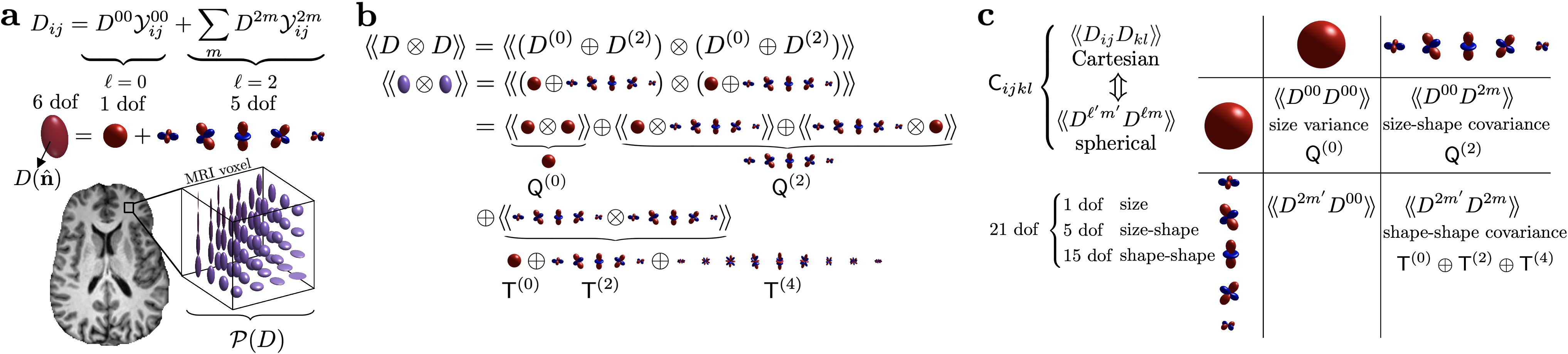
Figure 1: Outline: (a) An MRI voxel as a distribution $\mathcal{P}({D})$ of compartment diffusion tensors ${D}$ decomposed in the spherical tensor basis. (b) The QT decomposition of the covariance tensor $\mathsf{C}$ arises from the addition of “angular momenta”, Eq. (5): Central moments (2) of compartment tensors ${D}$ correspond to tensor products, subsequently averaged over the voxel-wise distribution $\mathcal{P}({D})$. (c) Irreducible components of the QT decomposition represent 1 size-size, 5 size-shape, and $1+5+9$ shape-shape covariances in the 21 dof of $\mathsf{C}$.

Our goal here is to study the geometry of the muti-dimensional dMRI signal beyond the diffusion tensor ellipsoid $\mathsf{D}(\hat{\mathbf{n}})\!=\!\mathsf{D}_{ij}n_{i}n_{j}$. (Einstein’s convention of summation over repeated Cartesian indices is assumed hereon.) We will construct the map between terms of the diffusion cumulant series [13, 14, 15] and the addition of “angular momenta” corresponding to the diffusion tensors of sub-voxel spin populations. While we study in detail the 4th-order covariance tensor $\mathsf{C}$, also relevant in materials science, elasticity and geology, our methodology can be further extended onto higher-order tensors.

The information content of the dMRI signal depends on the degree of coarse-graining [5, 7] over the diffusion length controlled by the diffusion time $t$. With sufficiently long $t\gtrsim 50\,\mathrm{ms}$ used in the clinic, each tissue compartment (a non-exchanging water population, e.g., intra-axonal space, extra-axonal space, etc) can be asymptotically considered as fully coarse-grained, such that diffusion in it becomes Gaussian [16, 17, 5]. Assuming (anisotropic) Gaussian diffusion in each compartment drastically simplifies the analysis. Indeed, the signal $S=\exp(-\mathop{\text{tr}}\mathsf{B}{D})$ (normalized to 1 in the absence of diffusion weighting) from any such “Gaussian compartment” defined by its diffusion tensor ${D}$, becomes fully encoded by a $3\times 3$ symmetric $\mathsf{B}$-tensor [18, 19, 20, 21, 15, 22]. The signal from a distribution $\mathcal{P}({D})$ of Gaussian compartments is then represented by the cumulant expansion [13, 14, 15]

$$\ln S=-\mathsf{B}_{ij}\,\mathsf{D}_{ij}+\tfrac{1}{2}\mathsf{B}_{ij}\mathsf{B}_{kl}\mathsf{C}_{ijkl}+{\cal O}(b^{3})\,,$$ (1)

where $b=\mathop{\text{tr}}\mathsf{B}$ is the $b$-value, cf. Materials and Methods, and

$$\mathsf{D}_{ij} =\left<{D}_{ij}\right>\,,$$ (2)

$$\mathsf{C}_{ijkl} =\left<\!\left<{D}_{ij}\,{D}_{kl}\right>\!\right>\equiv\left<\vphantom{a^{2}}\!\left({D}_{ij}-\langle{D}_{ij}\rangle\right)\left(\vphantom{\left<{D}_{ij}\right>}{D}_{kl}-\left<{D}_{kl}\right>\right)\right>$$

are components of the overall diffusion and covariance tensors $\mathsf{D}$ and $\mathsf{C}$ in an imaging voxel. Brackets $\left<\dots\right>$ denote averages over the diffusion tensor distribution $\mathcal{P}({D})$ that characterizes tissue in a given voxel, while double brackets $\left<\!\left<\dots\right>\!\right>$ denote cumulants [13]. Tensor $\mathsf{D}$ has 6 independent parameters, or “degrees of freedom” (dof), and $\mathsf{C}$ has 21 dof (Fig. 1).

A fundamental problem is to classify symmetries of the cumulant tensors in Eq. (1), and define tensor invariants, i.e., combinations of tensor components independent of the choice of basis (such as the trace $\mathsf{D}_{ii}$). With the advent of precision medicine and quantitative imaging [23], tensor invariants form a basis- and hardware-independent “fingerprint” of MRI signals [24, 25, 26, 27, 28, 29, 30]; their information content will underpin classifiers of pathology, development and aging [31]. A practical problem is to relate tensors and their invariants to tissue properties, and to design fast unbiased measurements.

Here we provide full classification of rotational invariants of the cumulant expansion (RICE) by decomposing tensors $\mathsf{D}$ and $\mathsf{C}$ according to irreducible representations of the SO(3) group of rotations. This reveals the cumulant tensors’ symmetries and geometric meaning, and connects with tissue biophysics embodied by the distribution $\mathcal{P}({D})$. All dMRI contrasts up to ${\cal O}(b^{2})$ (mean diffusivity (MD), fractional anisotropy (FA), mean, radial and axial kurtosis (MK, RK, AK), and microscopic FA ($\upmu$FA)), are expressed via just 7 RICE. Besides uncovering the 14 unexplored invariants, constructing RICE according to symmetries makes them “orthogonal”, and thereby potentially more specific to distinct microstructure changes.

Our geometric approach applies to hundreds of thousands publicly available human brain datasets [32, 33, 34, 35, 36]. We also derive the shortest iRICE protocols for mapping MD, FA, MK in 1 minute, and MD, FA, MK, $\upmu$FA in 2 minutes on a clinical scanner, making advanced dMRI clinically feasible.

Results

Warm-up: Irreducible decomposition of the diffusion tensor

Our main method of investigation will be the representation theory of SO(3) group applied to cumulant tensors (2). To set the stage, recall that a $3\times 3$ symmetric matrix, such as a diffusion tensor ${D}_{ij}$, splits into an isotropic component, $D^{(0)}_{ij}$, and a symmetric trace-free (STF) component, $D^{(2)}_{ij}$:

$${D}_{ij} =D^{(0)}_{ij}+D^{(2)}_{ij}={D}^{00}\mathcal{Y}^{00}_{ij}+\sum_{m=-2}^{2}{D}^{2m}\mathcal{Y}^{2m}_{ij}\,,$$ (3)

where $\mathcal{Y}^{\ell m}$ is a standard STF tensor basis such that $Y^{\ell m}(\hat{\mathbf{n}})=\mathcal{Y}^{\ell m}_{ij}n_{i}n_{j}$ are the spherical harmonics (SH) defined on a unit sphere $|\hat{\mathbf{n}}|=1$ [37]. Since $\sqrt{4\pi}\,\mathcal{Y}^{00}_{ij}=\delta_{ij}$ (unit matrix), the $\ell=0$ component yields the trace: ${D}^{00}/\sqrt{4\pi}=\tfrac{1}{3}\mathop{\text{tr}}{D}$. The $\ell=2$ sector contains 5 spherical tensor components ${D}^{2m}$ responsible for the shape and orientations of the diffusion tensor ellipsoid ${D}_{ij}n_{i}n_{j}$, while the single $\ell=0$ component ${D}^{00}$ (a scalar) sets its overall size.

Upon rotations, the spherical tensor components ${D}^{\ell m}$ with different $\ell$ do not mix: ${D}^{2m}$ transform amongst themselves; ${D}^{00}$ is an invariant. Mathematically, they belong to different irreducible representations of the SO(3) group [37, 38, 39]. Hence, Eq. (3) realizes the irreducible decomposition

$${D}=D^{(0)}\oplus D^{(2)}\,,\quad{D}^{(\ell)}\,=\,\{{D}^{\ell m}\}\,,\quad m=-\ell,\ldots,\ell\,,\ \$$ (4)

where each irreducible component of degree $\ell$ has $2\ell+1$ dof, such that the 6 dof of a symmetric $3\times 3$ matrix ${D}$ splits into $6=1+5$, cf. Fig. 1a. Spherical tensors will be our workhorse as they provide the natural way to represent tensors using the minimal number of dof. Furthermore, different transformation properties often point at distinct physical origins.

The diffusion tensor in Eq. (3) may describe a microscopic tissue compartment. Consider the invariants of ${D}$: the ellipsoid’s shape is defined by 3 semi-axes (the eigenvalues). The remaining 3 dof define its orientation in space (e.g., 3 Euler’s angles), and depend on the coordinate frame. The irreducible decomposition (4) allows one to construct tensor invariants symmetric with respect to the eigenvalues, and to assign the degree $\ell$ to them. The simplest, $\ell=0$ invariant, is the trace $\mathop{\text{tr}}D\propto D^{00}$. The remaining two independent $\ell=2$ invariants are also given by traces: $\mathop{\text{tr}}(D^{(2)})^{2}$ is proportional to the variance of the eigenvalues, and $\mathop{\text{tr}}(D^{(2)})^{3}=3\,\det D^{(2)}$ — to their product (readily seen in the eigenbasis of $D^{(2)}$).

The overall diffusion tensor $\mathsf{D}_{ij}$ is the mean of the compartment tensors (3) over $\mathcal{P}({D})$, cf. Eq. (2). Invariants of $\mathsf{D}$ give rise to common DTI metrics, such as MD, $\bar{\mathsf{D}}=\tfrac{1}{3}\mathop{\text{tr}}\mathsf{D}$ ($\ell=0$), and FA (from both $\ell=0$ and $\ell=2$ sectors, cf. Eq. (20) below).

The covariance tensor $\mathsf{C}$ involves averages of the direct tensor products ${D}\otimes{D}$, Eq. (2). To find the irreducible decomposition and the invariants of $\mathsf{C}$, in what follows we will construct a formal mapping onto the addition of quantum angular momenta with $\ell=0$ or $2$. This will relate the irreducible components of $\mathsf{C}$ to tissue properties via $\mathcal{P}({D})$, and to all previously studied model-independent dMRI metrics. We will then construct all invariants of $\mathsf{C}$ keeping track of their symmetries, relate them to dMRI measurements, and find ways of fast estimation of the most common invariants.

Size and shape covariances: QT decomposition

Using the irreducible decomposition (4) in Eq. (2) results in

$$\mathsf{C} =\left<\!\left<{D}\otimes{D}\right>\!\right>=\left<\!\left<\left(D^{(0)}\oplus D^{(2)}\right)\otimes\left(D^{(0)}\oplus D^{(2)}\right)\right>\!\right>$$ (5)

$$=\mathsf{Q}^{(0)}\oplus\mathsf{Q}^{(2)}\oplus\mathsf{T}^{(0)}\oplus\mathsf{T}^{(2)}\oplus\mathsf{T}^{(4)},$$

where

$$\mathsf{Q}^{(0)} =\left<\!\left<D^{(0)}\otimes D^{(0)}\right>\!\right>,$$ (6a)

$$\mathsf{Q}^{(2)} =2\left<\!\left<D^{(0)}\otimes D^{(2)}\right>\!\right>,$$ (6b)

$$\mathsf{T} =\left<\!\left<D^{(2)}\otimes D^{(2)}\right>\!\right>=\mathsf{T}^{(0)}\oplus\mathsf{T}^{(2)}\oplus\mathsf{T}^{(4)}.$$ (6c)

Formally, this corresponds to the addition of two quantum angular momenta with $\ell=0$ or $\ell=2$, see graphical representation in Fig. 1b. As it is known from quantum mechanics [38], addition of angular momenta $\vec{\ell_{1}}$ and $\vec{\ell_{2}}$ yields all possible states with momenta $\vec{L}$ between $|\ell_{1}-\ell_{2}|$ and $\ell_{1}+\ell_{2}$. Mathematically speaking [39], the tensor product $\ell_{1}\otimes\ell_{2}$ of representations labeled by $\ell_{1}$ and $\ell_{2}$ is reducible, and splits into a direct sum of irreducible representations with $L=|\ell_{1}-\ell_{2}|,\ \dots,\ \ell_{1}+\ell_{2}$. Successive terms in Eq. (5) symbolically yield the representations with the following angular momenta: $0\otimes 0=0$; $(0\otimes 2+2\otimes 0)=2$; and $2\otimes 2=0\oplus 2\oplus 4$. This yields the dof count for $\mathsf{C}$ tensor: $21=1+5+1+5+9$. In the $2\otimes 2$ case, we did not include representations with $\ell=1$ and $3$, forbidden by parity, $(-1)^{\ell}=+1$, coming from the time-reversal invariance of the Brownian motion.

Physically speaking, in a distribution $\mathcal{P}(D)$ of compartmental diffusion tensors of Fig. 1a, each ellipsoid (4) has an isotropic (“size”) part $D^{(0)}$ and trace-free anisotropic (“shape”) part $D^{(2)}$. Thus, the direct products in Eq. (6) define the size variance $\mathsf{Q}^{(0)}$, the size-shape covariance $\mathsf{Q}^{(2)}$, and the shape-shape covariance $\mathsf{T}$, Fig. 1b,c. The shape-shape covariance is reducible and further splits into three irreducible spherical tensors $\mathsf{T}^{(0)}$, $\mathsf{T}^{(2)}$ and $\mathsf{T}^{(4)}$.

Besides the explicit classification based on symmetries, the benefit of using spherical tensors is in having the minimal number of dof in each of them, as compared to the highly redundant Cartesian objects such as $\mathsf{C}_{ijkl}$. Therefore, one expects that the covariances $\left<\!\left<{D}^{\ell m}{D}^{\ell^{\prime}m^{\prime}}\right>\!\right>$ of the spherical-tensor components (4) of compartmental diffusivities should be related to the corresponding spherical-tensor components of $\mathsf{Q}$ and $\mathsf{T}$, Fig. 1c. We derive these explicit relations based on the spherical tensor algebra in Supplementary Section S3. In brief, the relations for $\mathsf{Q}$,

$$\mathsf{Q}^{00}=\tfrac{1}{\sqrt{4\pi}}\left<\!\left<({D}^{00})^{2}\right>\!\right>,\quad\mathsf{Q}^{2M}=\tfrac{2}{\sqrt{4\pi}}\left<\!\left<{D}^{00}{D}^{2M}\right>\!\right>$$ (7)

follow trivially from Eqs. (6a) and (6b). However, Eq. (6c)

$$\mathsf{T}^{LM} =\tfrac{5}{\sqrt{4\pi(2L+1)}}\braket{2,0,2,0}{L,0}$$ (8)

$$\times\sum_{m+m^{\prime}=M}\left<\!\left<{D}^{2m}{D}^{2m^{\prime}}\right>\!\right>\braket{2,m,2,m^{\prime}}{L,M}$$

involves the Clebsch-Gordan coefficients [38] $\braket{\ell,m,\ell^{\prime},m^{\prime}}{L,M}$ which obey the selection rule $M=m+m^{\prime}$ (and vanish otherwise). This rule makes the linear system (7)–(8) so sparse that it can be inverted by hand, see Supplementary Eq. (S11). This provides a full analytical solution for the tissue properties $\left<\!\left<{D}^{\ell m}{D}^{\ell^{\prime}m^{\prime}}\right>\!\right>$ in terms of the spherical components of $\mathsf{T}$ and $\mathsf{Q}$ tensors, i.e., the irreducible components of the covariance tensor $\mathsf{C}$. We call the above Eqs. (5)–(6) the QT decomposition of the covariance tensor.

Figure 2: Irreducible decompositions of $\mathsf{D}$ and $\mathsf{C}$ tensors, Eqs. (4), (6), and (13), for two white matter voxels: (a) corpus callosum — highly aligned fibers, and (b) longitudinal superior fasciculus — crossing fibers. Glyphs are rescaled to a similar size. They are color-coded by the sign (red = positive), while the radius represents the absolute value. (c) Representation of the eigentensor decomposition, Eq. (44) in Materials and Methods, of $\mathsf{T}^{(4)}$ for the crossing fiber voxel shown in (b). The 6 invariants of $\mathsf{T}^{(4)}=\mathsf{S}^{(4)}$ (cf. Fig. 3) correspond to 4 dof from $\lambda_{a}$ (here $\lambda_{4}=0$, $\mathsf{E}_{ij}^{(4)}\propto\delta_{ij}$, and $\sum_{a=1}^{6}\lambda_{a}=0$), and 2 dof defining the relative orientations among any pair of eigentensors $\mathsf{E}_{ij}^{(a)}$.

dMRI measurement: SA decomposition

dMRI parameter estimation is conventionally performed in a Cartesian basis. In what follows, we will construct the SA decomposition that is most natural for the dMRI acquisition, and derive how to proceed from SA to QT — i.e., from the acquisition to the tissue properties.

Historically, diffusion weightings in MR have been performed in a single direction using pulsed gradients [40], such that $\mathsf{B}_{ij}=b\,n_{i}n_{j}$ where $b=q^{2}t$; this so-called linear tensor encoding (LTE) corresponds to $\mbox{rank}\,\mathsf{B}=1$. As $\mathsf{B}_{ij}\mathsf{B}_{kl}\to b^{2}n_{i}n_{j}n_{k}n_{l}$ becomes symmetric in all indices, Eq. (1) becomes the diffusion kurtosis imaging (DKI) signal representation [41]:

$$\ln S=-b\,n_{i}n_{j}\,\mathsf{D}_{ij}+\tfrac{1}{2}b^{2}n_{i}n_{j}n_{k}n_{l}\,\mathsf{S}_{ijkl}+{\cal O}(b^{3})\,,$$ (9)

where $\mathsf{S}$, the fully symmetric part of $\mathsf{C}$, is proportional to the kurtosis tensor $\mathsf{W}$:

$$\mathsf{S}_{ijkl} \equiv\mathsf{C}_{(ijkl)}=\tfrac{1}{3}(\mathsf{C}_{ijkl}+\mathsf{C}_{iljk}+\mathsf{C}_{ikjl}),$$ (10)

$$\mathsf{W}_{ijkl} =\tfrac{3}{\bar{\mathsf{D}}^{2}}\,\mathsf{S}_{ijkl}\,,$$

and symmetrization over tensor indices between (…) is assumed henceforth [37]. Note the kurtosis tensor is made dimensionless by normalizing $\mathsf{S}$ with mean diffusivity squared.

Tensor $\mathsf{S}$ (likewise $\mathsf{W}$) splits into irreducible components with $\ell=0,\ 2,\ 4$. Their Cartesian components can be constructed by subtracting the corresponding traces [37]; equivalently, their spherical tensor components are found using Eqs. (33) in Materials and Methods. Thus, $\mathsf{S}^{(0)}$ is isotropic ($\ell=0$) and defined by 1 dof (the full trace $\mathsf{S}_{iijj}$ of $\mathsf{S}$), whereas $\mathsf{S}^{(2)}$ and $\mathsf{S}^{(4)}$ are STF tensors that are parametrized by $2\ell+1=5$ and $9$ dof, respectively, totalling $1+5+9=15$ dof for the kurtosis tensor.

The remaining $21-15=6$ dof of $\mathsf{C}$ are contained in the asymmetric (not antisymmetric!) part $\mathsf{A}$ of $\mathsf{C}$:

$$\mathsf{A}_{ijkl}=\mathsf{C}_{ijkl}-\mathsf{C}_{(ijkl)}\,=\tfrac{1}{3}(2\mathsf{C}_{ijkl}-\mathsf{C}_{iljk}-\mathsf{C}_{ikjl})\,.$$ (11)

To measure $\mathsf{A}$, the necessary (but not sufficient) condition is to use $\mbox{rank}\,\mathsf{B}>1$ [15]. Although $\mathsf{A}$ is a fourth-order tensor, it has 6 dof, and thus it is equivalent to a symmetric $3\times 3$ tensor [42, 43]:

$$\mathsf{A}_{pq} =\epsilon_{ikp}\epsilon_{jlq}\mathsf{A}_{ijkl}$$ (12a)

$$=\delta_{pq}(\mathsf{A}_{iikk}-\mathsf{A}_{ikik})+2(\mathsf{A}_{pkqk}-\mathsf{A}_{pqkk})\,,$$ (12b)

$$\mathsf{A}_{ijkl} =\tfrac{1}{6}(\epsilon_{ikp}\epsilon_{jlq}+\epsilon_{ilp}\epsilon_{jkq})\mathsf{A}_{pq}\,,$$ (12c)

where $\epsilon_{ijk}$ is the fully antisymmetric Levi-Civita tensor. Thus, analogously to Eq. (4), $\mathsf{A}$ splits into the irreducible components with $\ell=0$ and $2$.

To summarize, we can write the SA decomposition as:

$$\mathsf{C} =\mathsf{S}\oplus\mathsf{A}\,,$$ (13a)

$$\mathsf{S} =\mathsf{S}^{(0)}\oplus\mathsf{S}^{(2)}\oplus\mathsf{S}^{(4)}\,,$$ (13b)

$$\mathsf{A} =\mathsf{A}^{(0)}\oplus\mathsf{A}^{(2)}\,,$$ (13c)

where the dof count holds: $21_{\mathsf{C}}=(1+5+9)_{\mathsf{S}}+(1+5)_{\mathsf{A}}$. Due to this natural separation of information accessible through LTE ($\mathsf{S}$) vs non-LTE accessible ($\mathsf{A}$), we say the SA decomposition is acquisition-driven. Hundreds of thousands datasets acquired with LTE and moderate diffusion weightings are available [32, 33, 34, 35, 36] and thus, sensitive to the information present in $\mathsf{S}$ only.

The number of nonzero eigenvalues of the $\mathsf{B}$ tensor reflects how many dimensions of the diffusion process are being probed simultaneously. The requirement $\mbox{rank}\,\mathsf{B}>1$ means probing the diffusion along more than one dimension. In what follows, without the loss of generality, we focus on axially symmetric $\mathsf{B}$:

$$\mathsf{B}_{ij}(b,\beta,\hat{\mathbf{g}})=b\,\Big{(}\,\beta\,g_{i}g_{j}+\tfrac{1-\beta}{3}\,\delta_{ij}\Big{)}\,,$$ (14)

parametrized by its trace $b$ giving the overall scale; the unit vector $\hat{\mathbf{g}}$ along its symmetry axis; and the dimensionless shape parameter $\beta$ [44]. Compared to conventional LTE ($\beta=1$), varying $\beta$ changes the $\mathsf{B}$-tensor shape, e.g., $\beta=0$ for spherical tensor encoding (STE, isotropic $\mathsf{B}$-tensor), and $\beta=-\tfrac{1}{2}$ for planar encoding (PTE, two equal nonzero eigenvalues) [18, 19, 20, 21, 15, 22]. Non-axially symmetric $\mathsf{B}$-tensors are not necessary for accessing $\mathcal{O}(b^{2})$ information, and are typically not employed.

Non-LTE $\mathsf{B}$-tensors (14) probe the $\mathsf{A}$ tensor. Specifically, its contribution to the $b^{2}$ term in the cumulant expansion (1) can be expressed as

$$\tfrac{1}{2}\mathsf{B}_{ij}\mathsf{B}_{kl}\mathsf{A}_{ijkl}=\tfrac{b^{2}(1-\beta)(1+2\beta)}{27}\,\mathsf{A}_{pp}-\tfrac{b^{2}\beta(1-\beta)}{9}\,\mathsf{A}_{pq}g_{p}g_{q}\,,$$ (15)

a scalar $\propto\mathsf{A}^{00}=\tfrac{\sqrt{4\pi}}{3}\mathsf{A}_{pp}=\tfrac{\sqrt{4\pi}}{2}\mathsf{A}_{iikk}$ (full trace), plus an ellipsoid of the tensor (12a). As expected, Eq. (15) vanishes for LTE ($\beta=1$). STE ($\beta=0$) is sensitive only to the isotropic ($\ell=0$) part $\mathsf{A}^{00}$ (the scalar term), whereas PTE ($\beta=-\frac{1}{2}$) is the cleanest encoding to probe the $\mathsf{A}$ tensor ellipsoid: the first term vanishes, and the second term yields $+\tfrac{b^{2}}{12}\mathsf{A}_{pq}g_{p}g_{q}$.

From measurements (SA) to tissue properties (TQ)

Extracting tissue properties from $\mathsf{C}$ requires transforming $\mathsf{C}_{ijkl}$ into $\left<\!\left<{D}^{\ell m}{D}^{\ell^{\prime}m^{\prime}}\right>\!\right>$. First, we split $\mathsf{C}$ into $\mathsf{S}$ and $\mathsf{A}$ following Eqs. (10)-(11). Then, according to Eqs. (13), we compute the irreducible components $\mathsf{S}^{(\ell)}$ and $\mathsf{A}^{(\ell)}$, see explicit Eqs. (33) in Materials and Methods. Finally, a linear transformation, derived in Eqs. (35)–(37), relates the irreducible components of $\mathsf{T}^{(\ell)}$, $\mathsf{Q}^{(\ell)}$ with $\mathsf{S}^{(\ell)}$, $\mathsf{A}^{(\ell)}$:

$$\mathsf{Q}^{(0)} =\tfrac{5}{9}\,\mathsf{S}^{(0)}+\tfrac{2}{9}\,\mathsf{A}^{(0)}\,,$$ (16a)

$$\mathsf{Q}^{(2)} =\tfrac{7}{9}\,\mathsf{S}^{(2)}-\tfrac{2}{9}\,\mathsf{A}^{(2)}\,,$$ (16b)

$$\mathsf{T}^{(0)} =\tfrac{4}{9}\,\mathsf{S}^{(0)}-\tfrac{2}{9}\,\mathsf{A}^{(0)}\,,$$ (16c)

$$\mathsf{T}^{(2)} =\tfrac{2}{9}\,\mathsf{S}^{(2)}+\tfrac{2}{9}\,\mathsf{A}^{(2)}\,,$$ (16d)

$$\mathsf{T}^{(4)} =\mathsf{S}^{(4)}\,.$$ (16e)

Note that since each representation with $\ell=0$ and $\ell=2$ enters Eq. (5) twice, any decomposition with two independent linear combinations of representations with $\ell=0$, and separately for $\ell=2$, is equally legitimate. Here, the two decompositions (6) and (13) are selected by their distinct physical meaning: The SA decomposition is motivated by the acquisition and conventional parameter estimation, while the QT decomposition is natural to describe tissue properties. Upon rotations of the basis, the components $\mathsf{S}^{(\ell)},\mathsf{A}^{(\ell)}$, or $\mathsf{T}^{(\ell)},\mathsf{Q}^{(\ell)}$, transform such that they do not mix with each other.

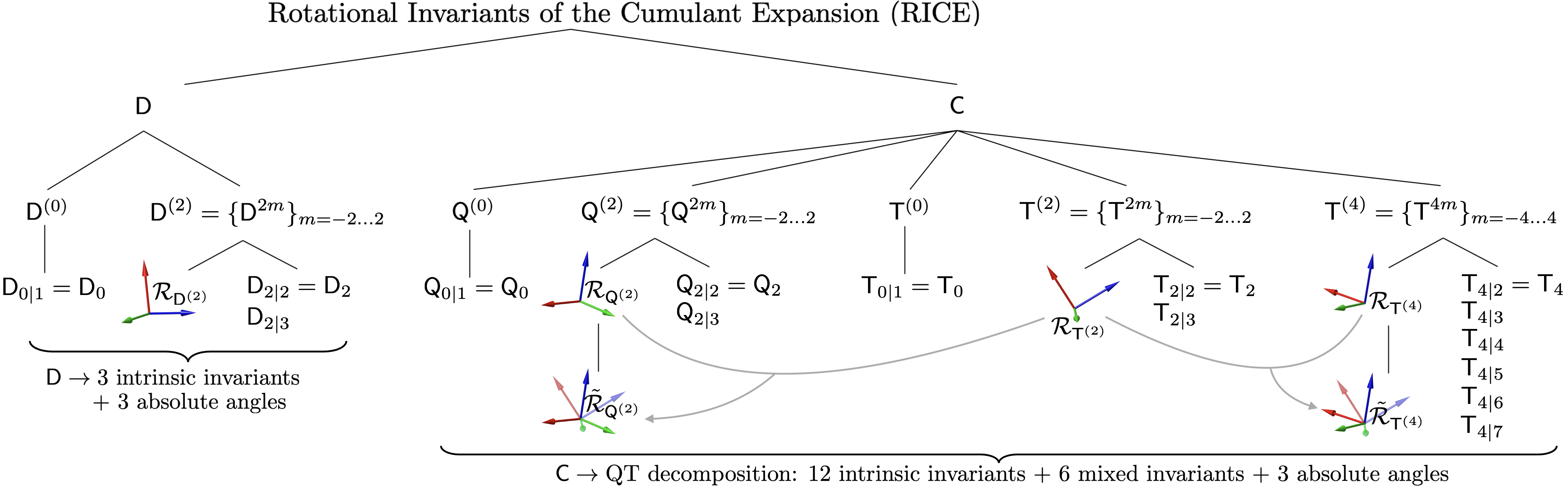
Figure 3: Irreducible decompositions of $\mathsf{D}$ and $\mathsf{C}$ (QT) tensors, Eqs. (4)–(5). Each irreducible component has its intrinsic invariants (1 for $\ell=0$; 2 for $\ell=2$; and 6 for $\ell=4$). Together with these $1+2+1+2+6=12$ intrinsic invariants, $\mathsf{C}$ has $3\cdot 3=9$ basis-dependent absolute angles defining the orientations of its $\mathsf{T}^{(2)}$, $\mathsf{T}^{(4)}$, and $\mathsf{Q}^{(2)}$ via the rotation matrices $\mathcal{R}_{\mathsf{Q}^{(2)}}$, $\mathcal{R}_{\mathsf{T}^{(2)}}$, and $\mathcal{R}_{\mathsf{T}^{(4)}}$, such that total dof count of $\mathsf{C}$ is $21=12+9$. Out of these 9 absolute angles, 6 dof are mixed invariants since they correspond to relative angles between $\mathsf{Q}^{(2)}$, $\mathsf{T}^{(2)}$ and $\mathsf{T}^{(4)}$. As an example, we take $\mathcal{R}_{\mathsf{T}^{(2)}}$ as a reference, and compute the relative rotations $\tilde{\mathcal{R}}_{\mathsf{T}^{(4)}}$ and $\tilde{\mathcal{R}}_{\mathsf{Q}^{(2)}}$. Maps of these invariants are shown in Fig. 4.

Geometric meaning

The geometric meaning of the irreducible decompositions such as (4), (6), and (13), comes from the correspondence between STF tensors and spherical harmonics (cf. Eq. (30) in Materials and Methods). For example, in the tensor glyphs of Fig. 2, $\mathsf{D}(\hat{\mathbf{n}})=\mathsf{D}_{ij}\,n_{i}n_{j}$, $\mathsf{Q}(\hat{\mathbf{n}})=\mathsf{Q}_{ij}\,n_{i}n_{j}$ and $\mathsf{T}(\hat{\mathbf{n}})=\mathsf{T}_{ijkl}\,n_{i}n_{j}n_{k}n_{l}$, where $\hat{\mathbf{n}}$ is a unit vector, the $\ell=0$ parts give directional averages. The $\ell=2$ parts are responsible for a glyph parametrized by five $Y^{2m}(\hat{\mathbf{n}})$, turning the corresponding ball into an ellipsoid, such as $\mathsf{D}(\hat{\mathbf{n}})=\mathsf{D}_{ij}n_{i}n_{j}$ in DTI [2].

The $\ell=0$ and $\ell=2$ parts can capture a single fiber tract (a single pair of opposite lobes on a sphere, both at the ${\cal O}(b)$ and ${\cal O}(b^{2})$ level), but cannot represent geometries with multiple pairs of lobes, such as in fiber crossings. The $\mathsf{T}^{(4)}=\mathsf{S}^{(4)}$ part, parametrized by nine $Y^{4m}(\hat{\mathbf{n}})$, is the only part of $\mathsf{C}$ that captures multiple pairs of lobes coming from fiber crossings, see Fig. 2c for an example. Interestingly, the beyond-LTE $\mathsf{A}$-tensor part of $\mathsf{C}$ can only accommodate an ellipsoidal glyph shape — albeit physically distinct from that of the diffusion tensor.

Irreducible components, such as $\mathsf{T}^{(\ell)}$ and $\mathsf{Q}^{(\ell)}$, have some dof whose values do not change upon rotations of the basis, i.e. are rotational invariant. The following subsection discusses how many rotational invariants we can find in $\mathsf{D}$ and $\mathsf{C}$ and how to compute them.

Invariants: intrinsic and mixed

We now construct all invariants of $\mathsf{C}$ in either QT or SA decomposition, by splitting them into the ones intrinsic to a given irreducible representation, and the ones mixing representations. Let us define intrinsic invariants as those that belong purely to a single irreducible component, such as $\mathsf{Q}^{(\ell)}$ and $\mathsf{T}^{(\ell)}$ in Eq. (6), or $\mathsf{S}^{(\ell)}$ and $\mathsf{A}^{(\ell)}$ in Eq. (13). Conversely, mixed invariants determine the relative orientations between different irreducible components with $\ell>0$, such as between $\mathsf{T}^{(2)}$ and $\mathsf{T}^{(4)}$. In what follows, we will focus on the invariants of the QT decomposition, Fig. 3, with all maps for a human brain shown in Fig. 4. An identical treatment yields the corresponding $\mathsf{S}$ and $\mathsf{A}$ invariants, cf. Supplementary Fig. S1.

Figure 4: RICE maps for a normal brain (33 y.o. male). Intrinsic invariants for each irreducible decomposition of $\mathsf{D}$, $\mathsf{T}$ and $\mathsf{Q}$ are shown as powers of corresponding traces, to match units of $\mathsf{D}$ and $\mathsf{C}$. The 6 mixed invariants correspond to Euler angles of eigenframes of $\mathsf{T}^{(4)}$ and $\mathsf{Q}^{(2)}$ relative to that of $\mathsf{T}^{(2)}$ (see text). The underlying tissue microstructure introduces correlations between invariants: e.g. small relative angles $\tilde{\beta}$ in white matter tracts exemplify the alignment of eigenframes of different representations of SO(3) with the tract.

How many intrinsic and mixed invariants exist? First note that the total number of invariants for any tensor equals its number of dof minus $3$ angles defining its overall orientation [45], yielding 3 for $\mathsf{D}$ (DTI), 12 for $\mathsf{S}$ or $\mathsf{W}$ (DKI), and 18 for $\mathsf{C}$. Applying this argument to each irreducible representation, the number of intrinsic invariants is 1 for $\ell=0$, and $(2\ell+1)-3=2(\ell-1)=2,\ 6,\ \dots$ for $\ell=2,\ 4,\ \dots\,$. This yields $(1+2+6)+(1+2)=12$ intrinsic invariants of $\mathsf{C}$, Fig. 3.

The isotropic, $\ell=0$ component of a symmetric tensor is a rotational invariant, which we normalize to its spherical mean:

$$\mathsf{D}_{0} =\mathsf{D}^{(0)}(\hat{\mathbf{n}})=\tfrac{1}{3}\,\mathrm{tr}\,\mathsf{D}=\tfrac{1}{3}\mathsf{D}_{ii}=C_{0}\,\mathsf{D}^{00}=\bar{\mathsf{D}}\,,$$ (17)

$$\mathsf{Q}_{0} =\mathsf{Q}^{(0)}(\hat{\mathbf{n}})=C_{0}\,\mathsf{Q}^{00}=\tfrac{5}{9}\,\mathsf{S}_{0}+\tfrac{2}{9}\,\mathsf{A}_{0}\,,$$

$$\mathsf{T}_{0} =\mathsf{T}^{(0)}(\hat{\mathbf{n}})=C_{0}\,\mathsf{T}^{00}=\tfrac{4}{9}\,\mathsf{S}_{0}-\tfrac{2}{9}\,\mathsf{A}_{0}\,,$$

where $C_{\ell}=\sqrt{\tfrac{2\ell+1}{4\pi}}$ and Eqs. (16a) and (16c) define relations between $\mathsf{A}_{0}\!=\tfrac{1}{3}\mathop{\text{tr}}\mathsf{A}=C_{0}\mathsf{A}^{00}$, $\mathsf{S}_{0}\!=\tfrac{1}{5}\mathop{\text{tr}}\mathsf{S}=C_{0}\mathsf{S}^{00}$, $\mathsf{Q}_{0}$, and $\mathsf{T}_{0}$.

Consider now the irreducible components with $\ell=2$. Among the 5 dof of tensors such as $\mathsf{D}^{(2)}$, $\mathsf{T}^{(2)}$ or $\mathsf{Q}^{(2)}$, 3 angles define the orientation (and are not invariants). The remaining 2 dof parametrize the three eigenvalues that sum up to zero trace. The corresponding 2 independent invariants can be written as:

$$\mathsf{D}_{2|{n}} =\left(\tfrac{2}{3}\,\mathrm{tr}(\mathsf{D}^{(2)})^{n}\right)^{1/n},\quad\,\,n=2,3,$$ (18)

and the same definition can be applied to $\mathsf{T}^{(2)}$, $\mathsf{Q}^{(2)}$, $\mathsf{S}^{(2)}$, and $\mathsf{A}^{(2)}$. For brevity, we dropped the $n=1$ index that indicates the power of the trace for $\ell=0$ in Eq. (17), and will from now on drop the $n=2$ index ($L_{2}$-norm) for $\ell\geq 2$. Thereby, the 3 invariants of $\mathsf{D}$: $\mathsf{D}_{0}=\mathsf{D}_{0|{1}}$, $\mathsf{D}_{2}\equiv\mathsf{D}_{2|{2}}$, and $\mathsf{D}_{2|{3}}$ (equivalent to its eigenvalues) determine the semi-axes of the corresponding ellipsoid; the same applies for $\mathsf{Q}^{(0)}\oplus\mathsf{Q}^{(2)}$, $\mathsf{T}^{(0)}\oplus\mathsf{T}^{(2)}$, and any second-order tensor.

For the $\ell=4$ components $\mathsf{T}^{(4)}=\mathsf{S}^{(4)}$, the picture is more complex. The 3 absolute angles determine the orientation of the glyph $\mathsf{T}^{(4)}(\hat{\mathbf{n}})$, while the remaining 6 dof are the invariants determining its shape (Fig. 2a,b). We construct these 6 intrinsic invariants in Materials and Methods and denote them

$$\mathsf{T}_{4|{n}} =\left(\tfrac{8}{35}\,\mathrm{tr}(\mathsf{T}^{(4)})^{n}\right)^{1/n},\quad n=2\dots 5\,;$$ (19)

$$\mathsf{T}_{4|{6}} ={\mathop{\text{tr}}}^{1/3}\mathsf{E}^{3}\,,\qquad\mathsf{T}_{4|{7}}={\mathop{\text{tr}}}^{1/3}\tilde{\mathsf{E}}^{3},$$

where $\mathsf{E}$ and $\tilde{\mathsf{E}}$ are defined in Eq. (46). The normalization coefficients $\tfrac{2}{3}$ and $\tfrac{8}{35}$ in Eqs. (18)–(19) are chosen to match the $L_{2}$-norms of their spherical components, as explained in Materials and Methods.

The relative angles between irreducible components of a given tensor do not change upon rotations (the tensor transforms as a whole). Hence, $18-12=6$ dof define the two sets of mixed invariants of $\mathsf{C}$ that parametrize the relative rotations between the frames of $\mathsf{T}^{(4)}$, $\mathsf{Q}^{(2)}$, and $\mathsf{T}^{(2)}$. Here, without the loss of generality, we take them as the Euler angles that define active rotations $\tilde{\mathcal{R}}_{\mathsf{T}}^{(4)}(\tilde{\alpha}_{\mathsf{T}}^{(4)},\tilde{\beta}_{\mathsf{T}}^{(4)},\tilde{\gamma}_{\mathsf{T}}^{(4)})$ and $\tilde{\mathcal{R}}_{\mathsf{Q}}^{(2)}(\tilde{\alpha}_{\mathsf{Q}}^{(2)},\tilde{\beta}_{\mathsf{Q}}^{(2)},\tilde{\gamma}_{\mathsf{Q}}^{(2)})$ of the $\mathsf{T}^{(2)}$ frame along $z$ by $\tilde{\alpha}$, then along new $x^{\prime}$ by $\tilde{\beta}$, and along new $z^{\prime\prime}$ by $\tilde{\gamma}$ to obtain the $\mathsf{T}^{(4)}$ and $\mathsf{Q}^{(2)}$ frames. Such mixed invariants are mapped for the human brain in the bottom row of Fig. 4 (cf. Supplementary Fig. S1 for $\mathsf{S}$ and $\mathsf{A}$ invariants).

Interestingly, $\mathsf{C}$ has the same symmetries of the elasticity tensor in continous media. However, our identification of invariants through irreducible representations and their corresponding symmetries makes our treatment distinct from that employed in the elasticity theory [46, 47, 48, 49, 50], and later in the dMRI context [51, 52, 53]. These previous works used Cartesian representations of $\mathsf{C}$ as a symmetric $6\times 6$ matrix (Kelvin or Voigt notation, cf. Eq. (42) in Materials and Methods). Here, the invariants were evaluated as coefficients of the generalized characteristic polynomial of two variables in the $6\times 6$ matrix representation of $\mathsf{C}$ [48, 51], or of the kurtosis tensor (10) [52], or through Hilbert’s theorem on non-negative ternary quartics to construct the invariants of $\mathsf{S}$ [53]. While formally yielding a number of invariants, these methods so far provided limited intuition for their geometric or physical meaning.

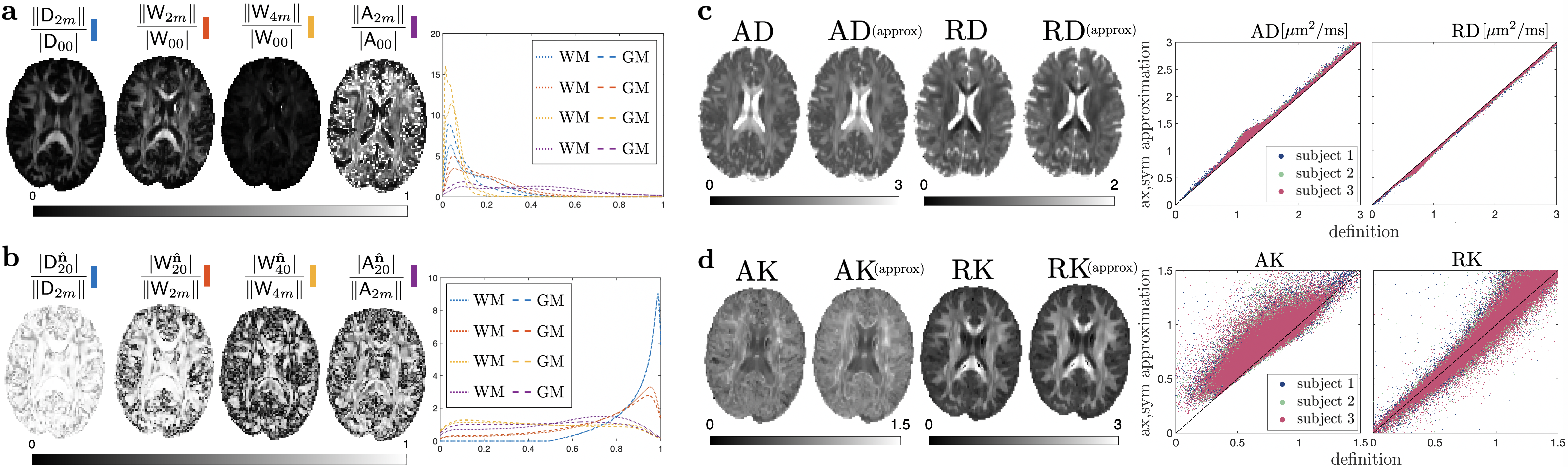
Figure 5: Significance of $\ell>0$ and axial symmetry in healthy brains. (a) Maps of the $L_{2}$-norms for degree-$\ell$ components of $\mathsf{D}$, $\mathsf{W}\propto\mathsf{S}$, and $\mathsf{A}$, and their histograms for white and gray matter voxels, normalized by $\ell=0$ components. $\mathsf{W}^{4m}$ elements are $5-10\times$ smaller than $\mathsf{W}^{00}$. (b) Relative contribution of the $m=0$ tensor components along the principal fiber axis $\hat{\mathbf{n}}$, normalized by the $L_{2}$-norm of all components with a given degree $\ell$; such ratio $=1$ for perfect axial symmetry. (c,d): Axial and radial projections of the diffusion (c) and kurtosis (d) tensors onto the principal fiber axis, with exact Eq. (52), and Eq. (53) relying on axial symmetry approximation.

Previously used dMRI contrasts from RICE

The 4 most widely used scalar dMRI contrasts can be expressed in terms of only 4 invariants. Two from DTI ($\mathsf{D}_{0}$, $\mathsf{D}_{2}$):

$$\text{MD}=\mathsf{D}_{0},\quad\text{FA}=\sqrt{\frac{3{\mathsf{D}_{2}}^{2}}{4{\mathsf{D}_{0}}^{2}+2{\mathsf{D}_{2}}^{2}}}\,,\\$$ (20)

and two from $\mathsf{C}$ ($\mathsf{S}_{0}$, $\mathsf{T}_{0}$):

$$\text{MK}=\frac{3\mathsf{S}_{0}}{{\mathsf{D}_{0}}^{2}},\quad\upmu\mathrm{FA}=\sqrt{\frac{15\mathsf{T}_{0}+3{\mathsf{D}_{2}}^{2}}{10\mathsf{T}_{0}+2{\mathsf{D}_{2}}^{2}+12{\mathsf{D}_{0}}^{2}}}\,,$$ (21)

where any pair of $\{\mathsf{T}_{0},\,\mathsf{Q}_{0},\,\mathsf{S}_{0},\,\mathsf{A}_{0}\}$ suffices, see Eq. (16).

Recently introduced isotropic [22, 15] and anisotropic [54, 55] variances

$$\mathbb{V}_{\mathrm{I}}=\mathsf{Q}_{0}\quad\text{and}\quad\mathbb{V}_{\mathrm{A}}=\mathsf{T}_{0}+\tfrac{1}{5}{\mathsf{D}_{2}}^{2}\,,$$ (22)

are expressed very naturally via $\mathsf{Q}_{0}$ and $\mathsf{T}_{0}$, respectively. As their names suggest, $\mathbb{V}_{\mathrm{I}}$ is related to the heterogeneity of isotropic compartmental tensor components $D^{(0)}$, whereas its counterpart $\mathbb{V}_{\mathrm{A}}$ is related to the heterogeneity of anisotropic compartmental components $D^{(2)}$. Both variances rely only on the $\ell=0$ invariants of $\mathsf{C}$. For a derivation of Eqs. (20)–(22) see Materials and Methods.

Empirically, the reason why $\ell=0$ invariants are the only ones explored so far, could be because the $\ell>0$ invariants are relatively smaller. Figure 5a shows “energy” ratios maps of $\ell=2,\,4$ invariants relative to $\ell=0$, together with histograms of gray and white matter voxels. It is evident that the contribution of high-order information in $\mathsf{D}$, $\mathsf{W}\propto\mathsf{S}$, and $\mathsf{A}$ decreases with the degree $\ell$ for both tissues. This is more pronounced in gray matter and less so in crossing fibers or highly aligned WM regions, e.g., the corpus callosum. In the kurtosis tensor, the 9 elements of $\ell=4$ are $\sim 5-10$ times smaller than MK.

For an axially-symmetric fiber tract, two more invariants are sometimes considered — axial and radial projections of $\mathsf{D}$ and $\mathsf{W}$ [56] (along and transverse to the fiber axis). In Eq. (53) of Materials and Methods, we express them via the above $\mathsf{D}_{0}$, $\mathsf{D}_{2}$, $\mathsf{S}_{0}$, together with $\mathsf{S}_{2}\equiv\mathsf{S}_{2|{2}}$ and $\mathsf{S}_{4}\equiv\mathsf{S}_{4|{2}}$, without the need to rotate to the basis aligned with the tract.

How good is the axial symmetry assumption for cumulant tensors? In Fig. 5b, we rotate all voxels’ principal fiber axes $\hat{\mathbf{n}}$ to $\hat{\mathbf{z}}$, and compute the relative fraction of “energy” along it. This is a measure of axial symmetry for each degree $\ell$, since axially symmetric tensors satisfy $|\mathsf{F}^{\ell 0}_{\hat{\mathbf{n}}}|/\|\mathsf{F}^{\ell m}\|\equiv 1$ for any $\ell$. This shows that $\mathsf{D}^{(2)}$ and $\mathsf{W}^{(2)}$ have a high axial symmetry, while the opposite holds for $\mathsf{W}^{(4)}$ and $\mathsf{A}^{(2)}$. Figures 5c and 5d show typical projections of the diffusion and kurtosis tensors onto the principal fiber basis, Eq. (52). These have a clear physical meaning when there is a predominant fiber direction in a voxel, in which case it makes sense to refer to them as axial or radial. Both figures show approximations that do not involve projecting onto the principal fiber basis, Eq. (53). These expressions are exact for axially symmetric tensors and show good agreement in the whole brain. This happens because, although $\mathsf{W}^{4m}$ may not be always axially symmetric, they are much smaller than $\mathsf{W}^{00}$ and $\mathsf{W}^{2m}$.

New invariants

Overall, just 6 independent invariants: $\mathsf{D}_{0}$ and $\mathsf{D}_{2}$; $\mathsf{S}_{0}$ and $\mathsf{A}_{0}$ (equivalently, $\mathsf{Q}_{0}$ and $\mathsf{T}_{0}$); and $\mathsf{S}_{2}$ and $\mathsf{S}_{4}$, are enough to synthesize all previously used dMRI contrasts up to ${\cal O}(b^{2})$ and hence clinically feasible. Since individual DTI eigenvalues may be used as contrasts, the total number of previously studied ${\cal O}(b^{2})$ invariants (explicitly or implicitly) is at most 3 from $\mathsf{D}$ ($\mathsf{D}_{0}$, $\mathsf{D}_{2}$, $\mathsf{D}_{2|{3}}$), and at most 4 from $\mathsf{C}$ ($\mathsf{A}_{0}$, $\mathsf{S}_{0}$, $\mathsf{S}_{2}$, $\mathsf{S}_{4}$).

The remaining 14 invariants of the $\mathsf{C}$ tensor contain essentially unexplored information. Their definition, symmetries, and geometric meaning constitute the main results of the present comprehensive group theory-based approach. For example, the size-shape correlation index of compartmental tensors, proportional to the norm of $\left<\!\left<{D}^{00}{D}^{2m}\right>\!\right>$ (Fig. 1e), introduced in Eq. (60) of Materials and Methods, involves invariants $\mathsf{Q}_{2}$, $\mathsf{Q}_{0}$ and $\mathsf{T}_{0}$. The $\ell=2$ and $\ell=4$ sectors of $\mathsf{T}$ have not been looked upon at all. The six mixed invariants relate to the underlying fiber tract geometry, quantifying correlations between eigenframes of different irreducible components.

The significance of these and other remaining RICE will be elucidated in future studies. Such a large set of complementary tissue contrasts is well suited for machine learning algorithms to study human development, aging and disease. Much like RGB pictures containing $N=3$ colors, the invariant maps with $N=21$ contrasts can be viewed as a large-$N$ generalization of computer vision data, prompting the development of large-$N$ classifiers.

For invariants not involving the $\mathsf{A}$ tensor, one can explore hundreds of thousands human data sets from imaging consortia such as the Alzheimer’s Disease Neuroimaging Initiative (ADNI) [32], Human Connectome Project [33], UK Biobank [35], and Adolescent Brain Cognitive Development (ABCD) [36], which are all compatible with the DKI signal representation. A comprehensive $\mathsf{B}$-tensor encoding human dataset has been recently made publicly available [57], from which all SA and QT invariants can be determined and studied.

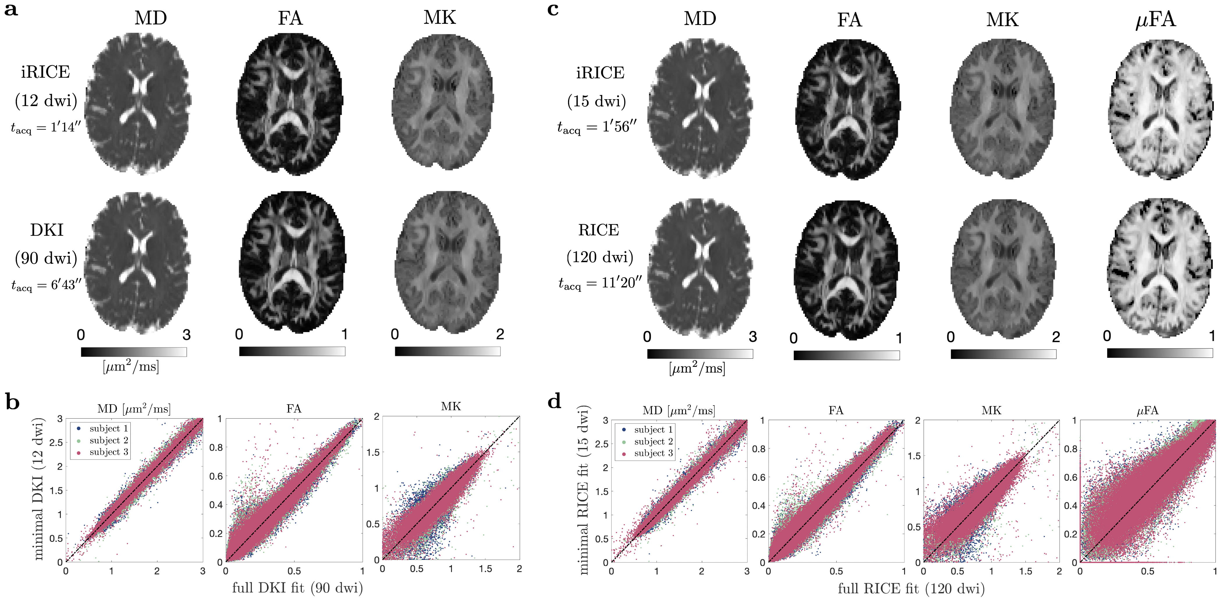
Figure 6: Comparison of iRICE (1-2 minutes) with fully sampled acquisitions (6-11 minutes). (a,c): iRICE maps (top) vs fully sampled DKI maps (bottom) for a healthy volunteer. Panels (b) and (d) show scatter plots for all brain voxels in 3 normal volunteers (3 colors).

Table 1: Comparison of existing and proposed fast protocols. Theoretically minimal protocols contain the minimum unique number of directions and distinct $b$-values (specific exemplary $b$-values can be altered). For STE, more than 1 direction implies rotation of the waveform for accuracy. All protocols include a non-diffusion weighted image ($b=0$).

Fast protocols comparison, $b$-values are in $\mathrm{ms}/\mathrm{\upmu m^{2}}$
Output maps	MD+MK	MD+FA+MK
Theoretical minimum	$6\!\times\!\mathrm{LTE}_{b=2}$	$6\!\times\!\mathrm{LTE}_{b=1};\,6\!\times\!\mathrm{LTE}_{b=2}$
	$1\!\times\!\mathrm{STE}_{b=1}$
iRICE (MD+FA+MK)		$6\!\times\!\mathrm{LTE}_{b=1};\,6\!\times\!\mathrm{LTE}_{b=2}$
Ref. [58]	$3\!\times\!\mathrm{LTE}_{b=1};\,9\!\times\!\mathrm{LTE}_{b=2}$
Output maps	MD+MK+$\bm{\upmu}$FA	MD+FA+MK+$\bm{\upmu}$FA
Theoretical minimum	$6\!\times\!\mathrm{LTE}_{b=2}$	$6\!\times\!\mathrm{LTE}_{b=1};\,6\!\times\!\mathrm{LTE}_{b=2}$
	$1\!\times\!\mathrm{STE}_{b=1};\,1\!\times\!\mathrm{STE}_{b=1.5}$	$1\!\times\!\mathrm{STE}_{b=1.5}$
iRICE (MD+FA+MK+$\upmu$FA)		$6\!\times\!\mathrm{LTE}_{b=1};\,6\!\times\!\mathrm{LTE}_{b=2}$
		$3\!\times\!\mathrm{STE}_{b=1.5}$
Ref. [59]	$3\!\times\!\mathrm{LTE}_{b=0.1};\,3\!\times\!\mathrm{LTE}_{b=0.7};\,6\!\times\!\mathrm{LTE}_{b=1.4};\,6\!\times\!\mathrm{LTE}_{b=2}$
	$6\!\times\!\mathrm{STE}_{b=0.1};\,6\!\times\!\mathrm{STE}_{b=0.7};\,10\!\times\!\mathrm{STE}_{b=1.4};\,16\!\times\!\mathrm{STE}_{b=2}$

Minimal protocols: iRICE

Table 1 shows the proposed minimal iRICE protocols to obtain MD, FA, MK, based on measurements with only 12 $\mathsf{B}$ tensors; and MD, FA, MK, $\upmu$FA with only 15 $\mathsf{B}$ tensors. These numbers are notably fewer than $21=6+15$ or $27=6+21$ necessary to determine all tensor components. These acquisition schemes involve fewer measurements than was previously anticipated [58]. Fast protocols from previous literature are shown for comparison.

In Materials and Methods we use spherical designs (special directions on a sphere) which guarantee that relevant tensor components are estimated, whereas components that do not contribute to the four invariants in Eq. (20)-(21) are canceled. In Supplementary Section S5 we prove that for the minimal protocols based on icosahedral directions, the tensor elements not involved in MD, FA, MK, $\upmu$FA explicitly cancel.

Minimal and fully sampled acquisitions were thoroughly compared. Maps for MD, FA, MK are shown in Fig. 6a and maps for MD, FA, MK, $\upmu$FA are shown in Fig. 6c. In both cases, minimal maps show a near-identical contrast to fully sampled maps despite having 8-fold fewer measurements and not estimating full tensors. Scatter plots, Figs. 6b,c, do not show biases. Regions where $\mathsf{W}_{4m}$ elements are larger, e.g., WM fiber crossings, show good correspondence in all maps.

Outlook

This work demonstrates how representation theory yields all symmetries and invariants of the diffusion and covariance tensors, and their geometric meaning. The generality of this approach extends our results to all fourth-order tensors with minor and major symmetries such as elasticity tensor in continuous media [46, 47, 48, 49, 50], yielding applications in mechanics, geology, materials science, and soft condensed matter physics. Higher-order cumulants [60], relevant for larger $b$ approaching the cumulant series’ convergence radius [61], are not used in clinic or clinical research so far. However, they can be classified using the present framework, by mapping onto the addition of 3 or more angular momenta, expanding on Eq. (8).

For diffusion NMR/MRI, we uncovered 14 invariants in addition to 7 previously used in the life sciences context of diagnostic MRI. Publicly available consortia dMRI datasets provide a place where the information of novel contrasts presented here can be exploited at a population level. RICE maps belong to distinct irreducible representations of rotations, and thereby represent “orthogonal” contrasts up to $b^{2}$. We hypothesize that this mutual independence may provide improved sensitivity and higher specificity to detect independent tissue microstructure changes in disease, aging and development. Additionally, we proposed two economic acquisition protocols (iRICE) requiring a minimal number of measurements for estimating MD, FA, MK, and $\upmu$FA. These minimal protocols have the potential to enable clinical translation of beyond-DTI diffusion metrics typically hampered due to long acquisition times.

Materials and Methods

Notations

Throughout this work, sans serif font refers to voxel-wise tensors, such as $\mathsf{D}$, $\mathsf{C}$, $\mathsf{A}$, $\mathsf{S}$, $\mathsf{Q}$, $\mathsf{T}$, whereas italic font refers to tensors ${D}$ of the microscopic compartments. These may have either Cartesian components such as $\mathsf{D}_{ij}$ and ${D}_{ij}$, or spherical tensor components such as $\mathsf{D}^{\ell m}$ and ${D}^{\ell m}$. We refer to irreducible components, such as $\mathsf{S}^{(\ell)}$, both as a collection of $\mathsf{S}^{\ell m}$ spherical tensor elements, or Cartesian ones $\mathsf{S}^{(\ell)}_{i_{1}\ldots i_{\ell}}$. Unless specified otherwise, the order $\ell$ of the latter will coincide with the number of Cartesian subindices since this is the most natural representation. We assume Einstein’s convention of summation over repeated Cartesian indices $ijkl...$.

Brackets $\left<\dots\right>$ denote averages over the compartmental diffusion tensor distribution $\mathcal{P}({D})$, and double brackets $\left<\!\left<\dots\right>\!\right>$ denote cumulants of $\mathcal{P}({D})$. Finally, for readability, we omit outer parentheses when referring to tensor traces, e.g., $\mathop{\text{tr}}\mathsf{B}=\mathop{\text{tr}}(\mathsf{B})$, $\mathop{\text{tr}}\mathsf{B}\mathsf{D}=\mathop{\text{tr}}(\mathsf{B}\mathsf{D})$, and $\mathop{\text{tr}}^{\nu}\mathsf{B}=\big{(}\mathop{\text{tr}}(\mathsf{B})\big{)}^{\nu}$.

Multiple Gaussian compartments

The dMRI signal from a given voxel

$$S=\langle e^{i\phi}\rangle_{\mathrm{paths+spins}}\,,\quad\phi=-\int_{0}^{t}\!\mathrm{d}\tau\,{\mathbf{g}}(\tau)\cdot\mathbf{r}(\tau)$$ (23)

is the transverse magnetization $e^{i\phi}$ in the rotating frame, averaged over all spins traveling along all possible Brownian paths $\mathbf{r}(\tau)$ between $\tau=0$ and measurement time $t$. Experiments are performed under the condition $\int_{0}^{t}{\mathbf{g}}(\tau)\,\mathrm{d}\tau=0$ on the applied Larmor frequency gradient ${\mathbf{g}}(\tau)$ [2, 17, 5]. In general, the dMRI signal is a functional of ${\mathbf{g}}(t)$, or, equivalently, of the encoding function ${\mathbf{q}}(t)=\int_{0}^{t}{\mathbf{g}}(t^{\prime})\,\mathrm{d}t^{\prime}$: $S=S[{\mathbf{q}}(t)]$. Even for a conventional pulsed-gradient diffusion sequence [40], one obtains a multi-dimensional phase diagram in the space of sequence parameters [8, 7].

However, after coarse-graining the dynamics over sufficiently long $t$, the microstructure-induced temporal velocity correlations become forgotten, such that the distribution of spin phase $\phi=\int_{0}^{t}\!\mathrm{d}\tau\,{\mathbf{q}}(\tau)\cdot\mathbf{v}(\tau)$ becomes asymptotically Gaussian, defined by its velocity autocorrelation function $\left<\!\left<v_{i}(\tau)v_{j}(\tau^{\prime})\right>\!\right>=2D_{ij}\,\delta(\tau-\tau^{\prime})$ [17, 5, 7]. The averaging in Eq. (23) is then represented in terms of the second cumulant of the phase, $S=e^{-\mathsf{B}_{ij}D_{ij}}$, and the measurement is determined by specifying the $\mathsf{B}$-tensor with elements

$$\mathsf{B}_{ij}=\int_{0}^{t}\!\mathrm{d}\tau\,q_{i}(\tau)\,q_{j}(\tau)$$ (24)

calculated based on ${\mathbf{q}}(t)$. The distribution $\mathcal{P}(D)$ of compartment diffusion tensors in a given voxel gives rise to the overall signal [62, 63, 64]

$$S(\mathsf{B})=\int\!\mathrm{d}D\,\mathcal{P}(D)\,e^{-\mathop{\text{tr}}\mathsf{B}D}=\sum_{\alpha}f_{\alpha}\,e^{-\mathop{\text{tr}}\mathsf{B}D^{\alpha}}\,.$$ (25)

Normalization $\int\!\mathrm{d}D\,\mathcal{P}(D)\!=\!1$ implies that the fractions add up to unity, $\sum_{\alpha}f_{\alpha}\!=\!1$.

Equation (25) is the most general form of a signal from multiple Gaussian compartments. It is valid when the transient processes have played out, such that compartmental diffusion tensors $D$ have all become time-independent, and thereby higher-order cumulants in each compartment are negligible [5]. In this case, the signal (25) is a function of the $\mathsf{B}$-tensor: $S[{\mathbf{q}}(t)]\to S(\mathsf{B})$, while tissue is fully represented by the voxelwise distribution $\mathcal{P}(D)$. This long-$t$ picture of multiple Gaussian compartments (anisotropic and non-exchanging) underpins a large number of dMRI modeling approaches, in particular, the Standard Model (SM) of diffusion [5] and its variants [65, 66, 67, 68, 69, 70]. Furthermore, this picture contains the SM extension onto different fiber populations in a voxel, lifting the key SM assumption of a single-fascicle “kernel” (response).

Given the forward model (25), an inverse problem is to restore $\mathcal{P}(D)$ from measurements with different $\mathsf{B}$. This problem is a matrix version of the inverse Laplace transform and is therefore ill-conditioned. Since in clinical settings, typical encodings are moderate ($\mathop{\text{tr}}\mathsf{B}\mathsf{D}\sim 1$), the inverse problem can be formulated term-by-term for the cumulant expansion (1) of the signal (25).

Parameter count in the cumulant series

The higher-order signal terms in Eq. (1) couple to successive cumulants of $\mathcal{P}(D)$. The inverse problem maps onto finding the cumulants $\left<\!\left<D_{i_{1}j_{1}}\dots D_{i_{n}j_{n}}\right>\!\right>$ (tensors of even order $2n$) from a set of measurements. This becomes obvious by noting the analogy $\mathsf{B}\to i\lambda$ with the standard cumulant series [13] $\ln p(\lambda)=\sum_{n=1}^{\infty}{(-i\lambda)^{n}\over n!}\left<\!\left<x^{n}\right>\!\right>$ for the characteristic function $p(\lambda)=\int\!\mathrm{d}x\,e^{-i\lambda x}p(x)$ of a probability distribution $p(x)$, such that the $n$-th term in Eq. (1) is $\frac{(-)^{n}}{n!}\mathsf{B}_{i_{1}j_{1}}\dots\mathsf{B}_{i_{n}j_{n}}\left<\!\left<D_{i_{1}j_{1}}\dots D_{i_{n}j_{n}}\right>\!\right>$.

Hence, the introduction of the $\mathsf{B}$-tensor, enabled by the Gaussian diffusion assumption, lowers the order by half: The $2n$-th cumulant of the phase (23) (the $2n$-th order term from expanding $\ln S[{\bf q}(t)]$ in ${\bf q}(t)$) maps onto the $n$-th cumulant $\left<\!\left<D_{i_{1}j_{1}}\dots D_{i_{n}j_{n}}\right>\!\right>$ of $\mathcal{P}(D)$ corresponding to the $n$-th order of expansion of $\ln S(\mathsf{B})$ in $\mathsf{B}$. The number of dof for this cumulant equals to that for a fully symmetric order-$n$ tensor of dimension $d=6$, which is a number of assignments of $n$ indistinguishable objects into $d$ distinguishable bins: $\binom{n+d-1}{n}=(n+5)!/(n!5!)=6,\ 21,\ 56,\ 126,\ \dots$ for $n=1,\ 2,\ 3,\ 4,\ \dots$ .

Irreducible representations of SO(3)

Here we remind key aspects from representation theory of SO(3) [38, 39] used throughout this work. A $d$-dimensional representation of a group is a mapping of each element (rotation) onto a $d\times d$ matrix that acts on a $d$-dimensional vector space. Representation theory provides a way to split a complex object (such as tensor $\mathsf{D}$ or $\mathsf{C}$) into a set of independent simpler ones with certain symmetries, on which a group acts. In particular, the elements of an irreducible representation transform among themselves, and hence can be studied separately.

All irreducible representations of SO(3) are labeled by their integer degree $\ell=0,\ 1,\ 2,\ \dots$, and have dimension $2\ell+1$. Each representation is formed, equivalently, by:

• $2\ell+1$ linearly independent Cartesian tensors $\mathsf{F}^{(\ell)}_{i_{1}\ldots i_{\ell}}$ of order $\ell$, which for $\ell>0$ are STF tensors. This means they are fully symmetric with respect to all $\ell!$ permutations of indices $i_{1}\ldots i_{\ell}$, and are trace-free, i.e., trace over arbitrary pair of indices is zero: $\mathsf{F}^{(\ell)}_{i_{1}\ldots i_{\ell}}\delta_{i_{n}i_{n^{\prime}}}\equiv 0$, $1\leq n,n^{\prime}\leq\ell$. The case of $\ell=0$ corresponds to a (generally nonzero) scalar;

• $2\ell+1$ spherical tensors $\mathsf{F}^{\ell m}$, $m=-\ell\dots\ell$, which are related to their STF counterparts via

  $$\mathsf{F}^{(\ell)}_{i_{1}\ldots i_{\ell}}=\sum_{m=-\ell}^{\ell}\mathsf{F}^{\ell m}\,\mathcal{Y}^{\ell m}_{i_{1}\ldots i_{\ell}}\,,$$ (26)

  where $\mathcal{Y}^{\ell m}_{i_{1}\ldots i_{\ell}}$ form the standard complex STF tensor basis [37] with Condon-Shortley phase [71]. Note that ${\mathsf{F}^{\ell m}}^{*}=(-1)^{m}\mathsf{F}^{\ell-m}$ for real-valued $\mathsf{F}^{(\ell)}_{i_{1}\ldots i_{\ell}}$.

Following Eq. (26), any arbitrary symmetric tensor can be represented as a sum of spherical tensors of different degrees:

$$\mathsf{F}_{i_{1}\ldots i_{L}} =\sum_{\ell=0}^{L}\mathsf{F}^{(\ell)}_{i_{1}\ldots i_{L}}=\sum_{\ell=0}^{L}\sum_{m=-\ell}^{\ell}\mathsf{F}^{\ell m}\,\mathcal{Y}^{\ell m}_{i_{1}\ldots i_{L}}\,,$$ (27)

where components of degree $\ell<L$ are uniquely mapped to an $L$-th order Cartesian tensor through symmetrization of the corresponding STF basis elements with sufficient number of kronecker symbols

$$\mathcal{Y}^{\ell m}_{i_{1}\ldots i_{L}}=\mathcal{Y}^{\ell m}_{(i_{1}\ldots i_{\ell}}\delta_{i_{\ell+1}i_{\ell+2}}\ldots\delta_{i_{L-1}i_{L)}}\,,\quad L\geq\ell\,.$$ (28)

As $\mathcal{Y}^{\ell m}_{i_{1}\ldots i_{\ell}}$ generate the set of $2\ell+1$ spherical harmonics

$$Y^{\ell m}(\hat{\mathbf{n}})=\mathcal{Y}^{\ell m}_{i_{1}\ldots i_{\ell}}\,n_{i_{1}}\ldots n_{i_{\ell}}=\mathcal{Y}^{\ell m}_{i_{1}\ldots i_{L}}n_{i_{1}}\ldots n_{i_{L}}\,,$$ (29)

for $m=-\ell\dots\ell$, the spherical tensor components transform upon SO(3) rotations as the SH components [37]. Both STF and SH representations generate identical “glyphs” (Fig. 2):

$$\mathsf{F}^{(\ell)}(\hat{\mathbf{n}})=\mathsf{F}^{(\ell)}_{i_{1}\ldots i_{\ell}}\,n_{i_{1}}\ldots n_{i_{\ell}}=\mathsf{F}^{\ell m}\,Y^{\ell m}(\hat{\mathbf{n}})\,.$$ (30)

Every degree $\ell$ in dMRI context are even due to time-reversal invariance of the Brownian motion dictating even parity $Y^{\ell m}(-\hat{\mathbf{n}})=Y^{\ell m}(\hat{\mathbf{n}})$. Hence, each cumulant or moment tensor, as in Eq. (1), can be split into a direct sum of irreducible representations with even $\ell$, connecting it with the orientation dispersion in the SH basis [29, 72].

Decomposition into irreducible representations

To find irreducible representations of $\mathsf{D}$ and $\mathsf{C}$, we need first to identify their symmetric components and subtract the traces. $\mathsf{D}$ is symmetric but $\mathsf{C}$ is not; thus, $\mathsf{C}$ must be first split into $\mathsf{S}$, its fully symmetric part, and $\mathsf{A}$, the remaining asymmetric part, following Eq. (10)-(11):

$$\mathsf{C}_{ijkl} =\mathsf{S}_{ijkl}+\mathsf{A}_{ijkl}\,,$$ (31a)

$$\mathsf{S}_{ijkl} =\mathsf{C}_{(ijkl)}=\tfrac{1}{3}(\mathsf{C}_{ijkl}+\mathsf{C}_{iljk}+\mathsf{C}_{ikjl})\,,$$ (31b)

$$\mathsf{A}_{ijkl} =\mathsf{C}_{ijkl}-\mathsf{C}_{(ijkl)}=\tfrac{1}{3}(2\mathsf{C}_{ijkl}-\mathsf{C}_{iljk}-\mathsf{C}_{ikjl})\,.$$ (31c)

To decompose $\mathsf{A}$, we use Eq. (12) from the main text, where Eq. (12a) is $\mathsf{A}_{pq}=4\Delta_{pq}$ from Eqs. (45)–(46) in [42]; here we use the same symbol $\mathsf{A}$ for 2nd and 4th order tensors, as they are isomorphic (and represent the same geometric object). Eq. (12b) is obtained by using the identity $\epsilon_{ijk}\epsilon_{lmn}=\delta_{il}\delta_{jm}\delta_{kn}+\delta_{im}\delta_{jn}\delta_{kl}+\delta_{in}\delta_{jl}\delta_{km}-\delta_{il}\delta_{jn}\delta_{km}-\delta_{in}\delta_{jm}\delta_{kl}-\delta_{im}\delta_{jl}\delta_{kn}$. Eq. (12c) (the inverse relation) follows from $\epsilon_{ijn}\epsilon_{kln}=\delta_{ik}\delta_{jl}-\delta_{il}\delta_{jk}$ and from the property $\mathsf{A}_{i(jkl)}\equiv 0$ that is a consequence of Eq. (11).

We now deal with fully symmetric Cartesian tensors $\mathsf{D}_{ij}$, $\mathsf{S}_{ijkl}$, and $\mathsf{A}_{ij}$, which can be represented as combinations of spherical tensors, cf. Eq. (27). To extract their spherical tensor components we rely on the orthogonality of such basis and project the Cartesian tensor onto the STF basis

$$\mathsf{F}^{\ell m}=\tfrac{4\pi\,L!}{(L+\ell+1)!!(L-\ell)!!}\,\mathsf{F}_{i_{1}\ldots i_{L}}\,\mathcal{Y}^{\ell m^{*}}_{i_{1}\ldots i_{\ell}}\delta_{i_{\ell+1}i_{\ell+2}}\ldots\delta_{i_{L-1}i_{L}}\,,\\$$ (32)

where $\ell!\equiv\ell(\ell-1)\cdot\cdot\cdot 2\cdot 1$, $\ell!!\equiv\ell(\ell-2)(\ell-4)\cdot\cdot\cdot(2\text{ or }1)$, and ^∗ denotes complex conjugation. The above normalization factor is derived in Supplementary Section S1, which agrees with [37] for $L=\ell$ since

$${\mathcal{Y}^{\ell m}_{i_{1}\ldots i_{\ell}}}^{*}\mathcal{Y}^{\ell m^{\prime}}_{i_{1}\ldots i_{\ell}}=\frac{(2\ell+1)!!}{4\pi\,\ell!}\,\delta_{mm^{\prime}}\,.$$

Applying Eq. (32) to obtain the spherical tensor elements $\mathsf{D}^{\ell m}$, $\mathsf{A}^{\ell m}$, and $\mathsf{S}^{\ell m}$ gives us

$$\mathsf{D}^{00} =\tfrac{4\pi}{3}\,C_{0}\,\mathsf{D}_{ii}\,\quad \mathsf{D}^{2m}=\tfrac{2\cdot 4\pi}{15}\,{\mathcal{Y}^{2m}_{ij}}^{*}\,\mathsf{D}_{ij}\,;$$ (33)

$$\mathsf{A}^{00} =\tfrac{4\pi}{3}\,C_{0}\,\mathsf{A}_{ii}\,,\quad \mathsf{A}^{2m}=\tfrac{2\cdot 4\pi}{15}\,{\mathcal{Y}^{2m}_{ij}}^{*}\,\mathsf{A}_{ij}\,;$$

$$\mathsf{S}^{00} =\tfrac{4\pi}{5}\,C_{0}\,\mathsf{S}_{iijj}\,,\quad \mathsf{S}^{2m}=\tfrac{4\cdot 4\pi}{35}\,{\mathcal{Y}^{2m}_{ij}}^{*}\,\mathsf{S}_{ijkk}\,,$$

$$\mathsf{S}^{4m} =\tfrac{8\cdot 4\pi}{315}\,{\mathcal{Y}^{4m}_{ijkl}}^{*}\,\mathsf{S}_{ijkl}\,.$$

Here we find it useful to define coefficients

$$C_{\ell}=\sqrt{\tfrac{2\ell+1}{4\pi}}\,.$$ (34)

From the above, one can compute the spherical tensor components of the QT decomposition following Eq. (16).

From tissue diffusivities to QT decomposition

We begin from the irreducible decomposition of compartmental diffusion tensors (3) used in $\mathsf{D}$ and $\mathsf{C}$, Eqs. (2):

$$\mathsf{D}_{ij} =\left<D^{00}\right>\mathcal{Y}_{ij}^{00}+\sum_{m}\left<D^{2m}\right>\mathcal{Y}_{ij}^{2m},$$ (35)

$$\mathsf{C}_{ijkl} =\left<\!\left<({D}^{00})^{2}\right>\!\right>\,\mathcal{Y}^{00}_{ij}\mathcal{Y}^{00}_{kl}$$

$$+\sum_{m}\left<\!\left<D^{00}D^{2m}\right>\!\right>\Big{(}\mathcal{Y}_{ij}^{00}\mathcal{Y}^{2m}_{kl}+\mathcal{Y}_{ij}^{2m}\mathcal{Y}^{00}_{kl}\Big{)}\,$$

$$+\sum_{m,m^{\prime}}\left<\!\left<D^{2m}D^{2m^{\prime}}\right>\!\right>\,\mathcal{Y}_{ij}^{2m}\mathcal{Y}_{kl}^{2m^{\prime}}\,.$$

Here the averages are taken over the distribution of compartmental diffusion tensors $\mathcal{P}({D})$. The $\ell=0$ component represents the trace of the compartmental tensors (size) and the $\ell=2$ components represent their shapes in a given reference frame, see Fig. 1a.

Next, Eqs. (10)-(11) enable us to compute the irreducible decompositions of $\mathsf{D}$ (trivial), $\mathsf{S}$, and $\mathsf{A}$, and group them according to their degree $\ell$:

$$\mathsf{D}^{00} =\left<\!\left<{D}^{00}\right>\!\right>\,,$$ (36)

$$\mathsf{S}^{00} =C_{0}\left<\!\left<({D}^{00})^{2}\right>\!\right>+C_{0}\textstyle\sum_{m}\left<\!\left<{{D}^{2m}}^{*}{D}^{2m}\right>\!\right>\,,$$

$$\mathsf{A}^{00} =2C_{0}\left<\!\left<({D}^{00})^{2}\right>\!\right>-\tfrac{5}{2}\,C_{0}\textstyle\sum_{m}\left<\!\left<{{D}^{2m}}^{*}{D}^{2m}\right>\!\right>\,,$$

$$\mathsf{D}^{2m} =\left<\!\left<D^{2m}\right>\!\right>\,,$$

$$\mathsf{S}^{2m} =2C_{0}\left<\!\left<D^{00}D^{2m}\right>\!\right>\!$$

$$+\!\tfrac{8}{21{C_{2}}^{2}}\textstyle\sum_{m^{\prime},m^{\prime\prime}}\left<\!\left<D^{2m^{\prime}}D^{2m^{\prime\prime}}\right>\!\right>\!\mathcal{Y}_{ij}^{2m^{\prime}}\mathcal{Y}_{jk}^{2m^{\prime\prime}}\mathcal{Y}_{ki}^{2m^{*}}\,,$$

$$\mathsf{A}^{2m} =\shortminus 2C_{0}\left<\!\left<D^{00}D^{2m}\right>\!\right>\!$$

$$+\!\tfrac{4}{3{C_{2}}^{2}}\textstyle\sum_{m^{\prime},m^{\prime\prime}}\left<\!\left<D^{2m^{\prime}}D^{2m^{\prime\prime}}\right>\!\right>\!\mathcal{Y}_{ij}^{2m^{\prime}}\mathcal{Y}_{jk}^{2m^{\prime\prime}}\mathcal{Y}_{ki}^{2m^{*}}\,,$$

$$\mathsf{S}^{4m} =\tfrac{8}{35{C_{4}}^{2}}\textstyle\sum_{m^{\prime},m^{\prime\prime}}\left<\!\left<D^{2m^{\prime}}D^{2m^{\prime\prime}}\right>\!\right>\mathcal{Y}_{ij}^{2m^{\prime}}\mathcal{Y}_{kl}^{2m^{\prime\prime}}\mathcal{Y}_{ijkl}^{4m^{*}}\,.$$

Equation (36) motivates $\mathsf{Q}$ and $\mathsf{T}$ definitions in Eq. (6), these cleanly separate the sources of different covariances:

$$\mathsf{Q}^{00} =C_{0}\left<\!\left<({D}^{00})^{2}\right>\!\right>\,,$$ (37)

$$\mathsf{Q}^{2m} =2C_{0}\left<\!\left<{D}^{00}{D}^{2m}\right>\!\right>\!\,,$$

$$\mathsf{T}^{00} =C_{0}\textstyle\sum_{m}\left<\!\left<{D}^{2m}{{D}^{2m}}^{*}\right>\!\right>\,,$$

$$\mathsf{T}^{2m} =\tfrac{8}{21{C_{2}}^{2}}\textstyle\sum_{m^{\prime},m^{\prime\prime}}\left<\!\left<{D}^{2m^{\prime}}{D}^{2m^{\prime\prime}}\right>\!\right>\!\mathcal{Y}_{ij}^{2m^{\prime}}\mathcal{Y}_{jk}^{2m^{\prime\prime}}\mathcal{Y}_{ki}^{2m^{*}}\,,$$

$$\mathsf{T}^{4m} =\tfrac{8}{35{C_{4}}^{2}}\textstyle\sum_{m^{\prime},m^{\prime\prime}}\left<\!\left<{D}^{2m^{\prime}}{D}^{2m^{\prime\prime}}\right>\!\right>\mathcal{Y}_{(ij}^{2m^{\prime}}\mathcal{Y}_{kl)}^{2m^{\prime\prime}}\mathcal{Y}_{ijkl}^{4m^{*}}\,.$$

It is straightforward to derive Eq. (16) from Eqs. (36)–(37). In particular, in the complex STF basis ${{D}^{\ell m}}^{*}=(-1)^{m}{D}^{\ell-m}$ since ${D}_{ij}$ is real-valued. Furthermore, $\mathcal{Y}_{ij}^{2m^{\prime}}\mathcal{Y}_{jk}^{2m^{\prime\prime}}{\mathcal{Y}_{ki}^{2m}}^{*}$ and $\mathcal{Y}_{ij}^{2m^{\prime}}\mathcal{Y}_{kl}^{2m^{\prime\prime}}{\mathcal{Y}_{ijkl}^{4m}}^{*}$ become proportional to the Clebsch-Gordan coefficients $\left<2,m^{\prime},2,m^{\prime\prime}|2,m\right>$ and $\left<2,m^{\prime},2,m^{\prime\prime}|4,m\right>$, see Supplementary Eq. (S9). This highlights how the relation between the $\mathsf{C}$ tensor and the covariances of compartmental diffusion tensors maps onto the addition of angular momenta (cf. Supplementary Section S3 for a detailed explanation).

Although the full QT system has 21 independent linear equations for 21 unknown covariances, it is sparse in two ways. First, $\ell=0$ equations are decoupled from $\ell>0$ ones. Thus, we do not need to fully measure $\mathsf{T}$ and $\mathsf{Q}$ to generate some of the typical diffusion contrasts that only depend on $\mathsf{T}^{00}$ and $\mathsf{Q}^{00}$. Second, most Clebsch-Gordan coefficients are zero due to the selection rule $m=m^{\prime}+m^{\prime\prime}$. This greatly simplifies Eq. (37), allowing for a clean analytical inversion of this system, see Supplementary Eq. (S11).

Intrinsic invariants

Degree $\ell=0$

For an arbitrary symmetric tensor $\mathsf{F}$ as in Eq. (27), we define its intrinsic $\ell=0$ invariant via either its $Y^{00}$ component in Eq. (30), or its full trace $\mathop{\text{tr}}\mathsf{F}=\mathsf{F}_{i_{1}i_{2}\ldots i_{\ell}}\delta_{i_{1}i_{2}}\ldots\delta_{i_{\ell-1}i_{\ell}}$:

$$\mathsf{F}_{0}\equiv\mathsf{F}_{0|1}=C_{0}\,\mathsf{F}^{00}=\tfrac{1}{\ell+1}\mathop{\text{tr}}\mathsf{F}\,,$$ (38)

since $\delta_{(i_{1}i_{2}}\ldots\delta_{i_{\ell-1}i_{\ell})}\delta_{i_{1}i_{2}}\ldots\delta_{i_{\ell-1}i_{\ell}}=\ell+1$. This normalization ensures $\mathsf{F}_{0}$ equals the average of $\mathsf{F}(\hat{\mathbf{n}})$ over the unit sphere.

Degree $\ell=2$

We focus on the invariants of $\mathsf{S}^{(2)}$, since $\mathsf{D}^{(2)}$, $\mathsf{A}^{(2)}$, $\mathsf{Q}^{(2)}$, and $\mathsf{T}^{(2)}$ can be treated analogously. The two intrinsic invariants for $\ell\!=\!2$ can be obtained from the characteristic equation [48]

$$\det(\mathsf{S}^{(2)}-\lambda\mathsf{I})=0\,,\quad\mathsf{I}_{ij}=\delta_{ij}\,,$$ (39)

since the coefficients of this cubic polynomial are rotationally invariant (note that $\mathop{\text{tr}}\mathsf{S}^{(2)}=0$). Using Eq. (18),

$$\mathsf{S}_{2} \equiv\mathsf{S}_{2|{2}}=\left(\tfrac{2}{3}\mathop{\text{tr}}(\mathsf{S}^{(2)})^{2}\right)^{1/2}\!=C_{2}(\mathsf{S}^{2m}{\mathsf{S}^{2m}}^{*})^{1/2}$$ (40)

$$={C_{2}}\left({|\mathsf{S}_{2-2}|}^{2}\!+\!{|\mathsf{S}_{2-1}|}^{2}\!+\!{|\mathsf{S}_{20}|}^{2}\!+\!{|\mathsf{S}_{21}|}^{2}\!+\!{|\mathsf{S}_{22}|}^{2}\right)^{1/2}\!,$$

$${\mathsf{S}_{2|{3}}} =\left(\tfrac{2}{3}\mathop{\text{tr}}(\mathsf{S}^{(2)})^{3}\right)^{1/3}\!=\left(2\,\mathrm{det}\mathsf{S}^{(2)}\right)^{1/3}$$

$$=\left(2\,\epsilon_{ijk}\mathsf{S}^{2m}\mathsf{S}^{2n}\mathsf{S}^{2p}\mathcal{Y}^{2m}_{1i}\mathcal{Y}^{2n}_{2j}\mathcal{Y}^{2p}_{3k}\right)^{1/3},$$

which have a 1-to-1 mapping to the eigenvalues of the matrix $\mathsf{S}^{(2)}_{ij}$ and $C_{2}$ is defined in Eq. (34). In the second equation above we used $\mathop{\text{tr}}(\mathsf{S}^{(2)})^{3}=3\,\det\mathsf{S}^{(2)}$ due to $\mathop{\text{tr}}\mathsf{S}^{(2)}=0$, which becomes obvious in the eigenbasis of $\mathsf{S}^{(2)}$. We discuss their normalization factor $\frac{2}{3}$ below, after $\ell=4$ invariants.

Degree $\ell=4$

Intrinsic invariants for fourth-order tensors are more intricate since we can write the characteristic equation with more dof than in the second-order case. For the covariance or elasticity tensor this can be written as [48]

$$\mathrm{det} \Big{(}\mathsf{C}-\mathsf{I^{(4)}}(\lambda,\mu)\Big{)}=0,$$ (41)

$$\mathsf{I}_{ijkl}^{(4)}(\lambda,\mu) =\tfrac{\lambda}{2}(\delta_{ik}\delta_{jl}+\delta_{il}\delta_{jk})+\mu\,\delta_{ij}\delta_{kl}.$$

To solve this problem, Refs. [48, 51] and others proposed to map the elasticity fourth-order 3D tensor to a second-order 6D tensor. For $\mathsf{C}\rightarrow\mathsf{C}_{6\times 6}$ one uses the mapping [51]:

$$\left(\begin{array}[]{cccccc}\!\!{\scriptstyle\mathsf{C}_{1111}}&{\scriptstyle\mathsf{C}_{1122}}&{\scriptstyle\mathsf{C}_{1133}}&{\scriptstyle\sqrt{2}\,\mathsf{C}_{1112}}&{\scriptstyle\sqrt{2}\,\mathsf{C}_{1113}}&{\scriptstyle\sqrt{2}\,\mathsf{C}_{1123}\vspace{0.1cm}}\\ \vspace{0.1cm}{\scriptstyle\mathsf{C}_{1122}}&{\scriptstyle\mathsf{C}_{2222}}&{\scriptstyle\mathsf{C}_{2233}}&{\scriptstyle\sqrt{2}\,\mathsf{C}_{2212}}&{\scriptstyle\sqrt{2}\,\mathsf{C}_{2213}}&{\scriptstyle\sqrt{2}\,\mathsf{C}_{2223}}\\ \vspace{0.1cm}{\scriptstyle\mathsf{C}_{1133}}&{\scriptstyle\mathsf{C}_{2233}}&{\scriptstyle\mathsf{C}_{3333}}&{\scriptstyle\sqrt{2}\,\mathsf{C}_{3312}}&{\scriptstyle\sqrt{2}\,\mathsf{C}_{3313}}&{\scriptstyle\sqrt{2}\,\mathsf{C}_{3323}}\\ \vspace{0.1cm}{\scriptstyle\sqrt{2}\,\mathsf{C}_{1112}}&{\scriptstyle\sqrt{2}\,\mathsf{C}_{2212}}&{\scriptstyle\sqrt{2}\,\mathsf{C}_{3312}}&{\scriptstyle 2\,\mathsf{C}_{1212}}&{\scriptstyle 2\,\mathsf{C}_{1213}}&{\scriptstyle 2\,\mathsf{C}_{1223}}\\ \vspace{0.1cm}{\scriptstyle\sqrt{2}\,\mathsf{C}_{1113}}&{\scriptstyle\sqrt{2}\,\mathsf{C}_{2213}}&{\scriptstyle\sqrt{2}\,\mathsf{C}_{3313}}&{\scriptstyle 2\,\mathsf{C}_{1312}}&{\scriptstyle 2\,\mathsf{C}_{1313}}&{\scriptstyle 2\,\mathsf{C}_{1323}}\\ \vspace{0.1cm}{\scriptstyle\sqrt{2}\,\mathsf{C}_{1123}}&{\scriptstyle\sqrt{2}\,\mathsf{C}_{2223}}&{\scriptstyle\sqrt{2}\,\mathsf{C}_{3323}}&{\scriptstyle 2\,\mathsf{C}_{2312}}&{\scriptstyle 2\,\mathsf{C}_{2313}}&{\scriptstyle 2\,\mathsf{C}_{2323}}\end{array}\!\!\right).$$ (42)

The characteristic polynomial in Eq. (41) has degree 6 in $\lambda$ and degree 3 in $\mu$ [48]. From these coefficients, one can extract $\mathsf{C}$ invariants; however, they mix different irreducible representations.

In this work, to keep track of distinct symmetries, we propose to use Eq. (41) to solve a more constrained problem: finding the intrinsic invariants of $\mathsf{S}^{(4)}$, which has only 9 independent parameters. The corresponding $6\times 6$ equation ${\mathsf{S}^{(4)}}_{6\times 6}$ is spelled out in Section S6 of Supplementary Material. The characteristic polynomial is sixth-order in $\lambda$ and first-order in $\mu$. Remarkably, it has only 4 nonzero independent roots, which can be found by setting $\mu=0$. These have a 1-to-1 mapping with the eigenvalues of $\mathsf{\mathsf{S}^{(4)}}_{6\times 6}$, or equivalently, $\mathop{\text{tr}}(\mathsf{S}^{(4)})^{n},\,n=1,\ldots,6$. Thus, the natural way of constructing the invariants is to consider the traces $\mathop{\text{tr}}(\mathsf{S}^{(4)})^{n}$. Note that

$$\mathop{\text{tr}}(\mathsf{S}^{(4)})^{n}=\mathsf{S}^{(4)}_{i_{1}j_{1}i_{2}j_{2}}\ldots\mathsf{S}^{(4)}_{i_{n}j_{n}i_{1}j_{1}}=\mathop{\text{tr}}(\mathsf{S}^{(4)}_{6\times 6})^{n}.$$ (43)

Since by Cayley–Hamilton theorem, each matrix satisfies its characteristic equation (in this case, of the order 6), and $\mathop{\text{tr}}\mathsf{S}^{(4)}=0$, the traces $\mathop{\text{tr}}(\mathsf{S}^{(4)})^{2}$, $\mathop{\text{tr}}(\mathsf{S}^{(4)})^{3}$, $\mathop{\text{tr}}(\mathsf{S}^{(4)})^{4}$, and $\mathop{\text{tr}}(\mathsf{S}^{(4)})^{5}$ determine all traces of higher powers of $\mathsf{S}^{(4)}$. They are normalized in Eq. (19) of the main text according to Eq. (47).

The remaining 2 intrinsic invariants of $\mathsf{S}^{(4)}$ can be obtained from its eigentensor decomposition [51]

$$\mathsf{S}_{ijkl}^{(4)}=\sum_{a=1}^{6}\lambda_{a}\mathsf{E}_{ij}^{(a)}\mathsf{E}_{kl}^{(a)},$$ (44)

where $\lambda_{a}$ and $\mathsf{E}_{ij}^{(a)}$ are the eigenvalues and eigentensors of $\mathsf{S}^{(4)}$. This is analogous to an eigenvalue decomposition of ${\mathsf{S}^{(4)}}_{6\times 6}$ akin to Eq. (41) with $\mu=0$. Here, $\lambda_{a}$ are the eigenvalues and $\hat{\mathbf{v}}^{(a)}=[v^{(a)}_{xx},\,v^{(a)}_{yy},\,v^{(a)}_{zz},\,v^{(a)}_{xy},\,v^{(a)}_{xz},\,v^{(a)}_{yz}]$ are the normalized eigenvectors, from which we build

$$\mathsf{E}_{ij}^{(a)}=\left(\begin{array}[]{ccc}v_{xx}^{(a)}&\frac{1}{\sqrt{2}}v_{xy}^{(a)}&\frac{1}{\sqrt{2}}v_{xz}^{(a)}\\ \frac{1}{\sqrt{2}}v_{xy}^{(a)}&v_{yy}^{(a)}&\frac{1}{\sqrt{2}}v_{yz}^{(a)}\\ \frac{1}{\sqrt{2}}v_{xz}^{(a)}&\frac{1}{\sqrt{2}}v_{yz}^{(a)}&v_{zz}^{(a)}\end{array}\right).$$ (45)

Eigentensors satisfy $\mathsf{E}^{(a)}_{ij}\mathsf{E}^{(b)}_{ij}=\delta_{ab}$. From direct inspection of ${\mathsf{S}^{(4)}}_{6\times 6}$ (cf. Supplementary Section S6) it can be seen that the eigentensor associated with a zero eigenvalue, $\lambda_{a_{0}}\!=\!0$, is $\mathsf{E}^{(a_{0})}_{ij}=\tfrac{1}{\sqrt{3}}\delta_{ij}$, $\hat{\mathbf{v}}^{(a_{0})}=\tfrac{1}{\sqrt{3}}\,(1,\,1,\,1,\,0,\,0,\,0)^{t}$. Furthermore, $\mathop{\text{tr}}\mathsf{E}^{(a)}=0$ for all other five eigentensors $a\neq a_{0}$.

To obtain the remaining two invariants of $\mathsf{S}^{(4)}$, one must utilize the eigentensors. We define

$$\mathsf{E}_{ij}=\sum_{a}\lambda_{a}\mathsf{E}_{ij}^{(a)},\quad\text{and}\quad\tilde{\mathsf{E}}_{ij}=\sum_{a\neq a_{0}}\mathsf{E}_{ij}^{(a)}.$$ (46)

Traces of powers of $\mathsf{E}$ and $\tilde{\mathsf{E}}$ are rotationally invariant. As for any second-order tensor, only traces of linear, quadratic and cubic powers of these matrices are algebraically independent. Further, by construction, $\mathop{\text{tr}}\mathsf{E}=\mathop{\text{tr}}\tilde{\mathsf{E}}=0$. One can also check that $\mathop{\text{tr}}\mathsf{E}^{2}=\mathop{\text{tr}}(\mathsf{S}^{(4)})^{2}$ and $\mathop{\text{tr}}\tilde{\mathsf{E}}^{2}=5$, which is given by one of the previously found invariants. Therefore, we identify the two remaining independent intrinsic invariants of $\mathsf{S}^{(4)}$ with $\mathop{\text{tr}}\mathsf{E}^{3}$ and $\mathop{\text{tr}}\tilde{\mathsf{E}}^{3}$. We denoted these six intrinsic invariants $\mathsf{S}_{4|{n}},\,n=2\dots 7$, in Eq. (19).

It is fairly natural to assign meaning to $\mathsf{S}_{4|{n}},\,n=2\ldots 5$, since these can be seen as shape tensor metrics of increasing order. For $\mathsf{S}_{4|{6}}=\mathop{\text{tr}}\mathsf{E}^{3}$ and $\mathsf{S}_{4|{7}}=\mathop{\text{tr}}\tilde{\mathsf{E}}^{3}$ this is less intuitive. Thus, one alternative is to take any pair of eigentensors, say $\mathsf{E}_{ij}^{(6)}$ and $\mathsf{E}_{ij}^{(5)}$ (where $\lambda_{6}$ is the largest and $\lambda_{5}$ is the second largest eigenvalue), and compute the 3d rotation matrix between their bases, $\mathcal{R}_{5,6}$, see Supplementary Fig. 2. Such rotation matrix has three important aspects: (i) it contains independent information to that provided by the eigenvalues (although it is affected by $\{\lambda_{a}\}$); (ii) it is invariant to overall rotations of $\mathsf{S}^{(4)}$; (iii) even though it seems to have 3 free parameters, after fixing $\{\lambda_{a}\}$ values we can observe that $\mathcal{R}_{5,6}$ is parametrized by two degrees of freedom $\varphi$ and $\psi$. These have a nontrivial relation with $\mathsf{S}_{4|{6}}$ and $\mathsf{S}_{4|{7}}$.

Normalization

Intrinsic invariants are defined such that their units match those of tensor elements, except for $\mathsf{S}_{4|{7}}=\mathop{\text{tr}}\tilde{\mathsf{E}}^{3}$ that is dimensionless. Normalization coefficients for $n$-th power traces, $\mathop{\text{tr}}(\mathsf{S}^{(\ell)})^{n}$ with $\ell>0$, depend on $\ell$, e.g. $\tfrac{2}{3}$ for $\ell=2$ in Eq. (18). These factors are chosen such that $n=2$ invariants match the $L_{2}$-norms over $m$ for $\mathsf{S}^{\ell m}$:

$${\mathsf{S}_{\ell}}^{2}\equiv{\mathsf{S}_{\ell|2}}^{2}\equiv C_{\ell}^{2}\!\sum_{m=-\ell}^{\ell}\!|\mathsf{S}^{\ell m}|^{2}=\frac{\ell!}{(2\ell-1)!!}\mathop{\text{tr}}(\mathsf{S}^{(\ell)})^{2}\,,$$ (47)

where $\mathop{\text{tr}}(\mathsf{S}^{(\ell)})^{2}=\mathsf{S}^{(\ell)}_{i_{1}\ldots i_{\ell/2}j_{\ell/2+1}\ldots j_{\ell}}\mathsf{S}^{(\ell)}_{j_{\ell/2+1}\ldots j_{\ell}i_{1}\ldots i_{\ell/2}}$. Equations (17)–(19) correspond to specific cases of $\ell=0,2,4$.

Conventional contrasts from RICE

MD, FA, and MK

Interestingly, the first four equations in Eq. (36) are decoupled from the others. Forming the $\mathsf{D}_{0}$ and $\mathsf{D}_{2}$ invariants as in Eq. (17)-(18), we can compute:

MD $$\equiv\bar{\mathsf{D}}=\tfrac{1}{4\pi}\int_{\mathbb{S}^{2}}\!\mathsf{D}(\hat{\mathbf{n}})\,\mathrm{d}\hat{\mathbf{n}}=\tfrac{1}{3}\mathop{\text{tr}}\mathsf{D}=\mathsf{D}_{0},$$ (48a)

$$\text{FA}^{2} =\frac{3}{2}\frac{{\mathbb{V}_{\lambda}(\mathsf{D})}}{{\mathbb{V}_{\lambda}(\mathsf{D})}+3\bar{\mathsf{D}}^{2}}=\frac{3{\mathsf{D}_{2}}^{2}}{4{\mathsf{D}_{0}}^{2}+2{\mathsf{D}_{2}}^{2}},$$ (48b)

where $\mathsf{D}(\hat{\mathbf{n}})=\mathsf{D}_{ij}n_{i}n_{j}$ and

$$\mathbb{V}_{\lambda}(\mathsf{D})\equiv\tfrac{1}{3}\sum_{i=1}^{3}(\lambda_{i}-\bar{\mathsf{D}})^{2}=\tfrac{1}{2}{C_{2}}^{2}\textstyle\sum_{m}\mathsf{D}^{2m}\,{\mathsf{D}^{2m}}^{*}=\tfrac{1}{2}{D_{2}}^{2}$$ (49)

is the variance of the set of 3 eigenvalues of any second-order tensor in 3 dimensions, such as $\mathsf{D}$. The relation for FA becomes evident if we realize that in the eigenbasis, $\mathsf{D}^{(2)}=\mathrm{diag}(\lambda_{1}-\bar{\mathsf{D}},\lambda_{2}-\bar{\mathsf{D}},\lambda_{3}-\bar{\mathsf{D}})$. Thus, the rotational invariant ${\mathsf{D}_{2}}^{2}=2\mathbb{V}_{\lambda}(\mathsf{D})$ [29]. Although the dimensionless ratio $\mathsf{D}_{2}/\mathsf{D}_{0}$ would be perhaps a more natural way to quantify the anisotropy of $\mathsf{D}$, historically FA has been the preferred way to do so due to bounding it to $[0,1]$ interval by placing $\mathbb{V}_{\lambda}(\mathsf{D})$ in the denominator, which however makes its statistical properties less transparent.

The definition of mean kurtosis is ambiguous in the dMRI literature. In this work we define MK as the angular average of the dimensionless cumulant tensor $\mathsf{W}(\hat{\mathbf{n}})$ [73, 58, 74]:

$$\mathrm{MK}\equiv\bar{\mathsf{W}}=\!\tfrac{1}{4\pi}\!\int_{\mathbb{S}^{2}}\!\!\mathsf{W}(\hat{\mathbf{n}})\mathrm{d}\hat{\mathbf{n}}\!=\!\tfrac{1}{5}\mathsf{W}_{iijj}\!=\!\tfrac{1}{5}\mathop{\text{tr}}\mathsf{W}\!=\!\mathsf{W}_{0},$$ (50)

where $\mathsf{W}(\hat{\mathbf{n}})=\mathsf{W}_{ijkl}n_{i}n_{j}n_{k}n_{l}$. $\bar{\mathsf{W}}$ can be computed fast and precisely from the estimated $\mathsf{W}$ tensor by simply taking a full trace which is proportional to the principal invariant $\mathsf{W}_{0}$.

The original DKI paper [41] defined mean kurtosis as the angular average of the directional kurtosis $K({\bf\hat{n}})$:

$$K({\bf\hat{n}})=\frac{\bar{\mathsf{D}}^{2}\mathsf{W}(\hat{\mathbf{n}})}{\mathsf{D}^{2}(\hat{\mathbf{n}})},\,\,\bar{K}=\tfrac{1}{4\pi}\!\int_{\mathbb{S}^{2}}\!\!\mathrm{d}\hat{\mathbf{n}}\,K(\hat{\mathbf{n}})=\tfrac{\bar{\mathsf{D}}^{2}}{4\pi}\!\int_{\mathbb{S}^{2}}\!\!\mathrm{d}\hat{\mathbf{n}}\,\frac{\mathsf{W}(\hat{\mathbf{n}})}{\mathsf{D}^{2}(\hat{\mathbf{n}})}.$$ (51)

Note that both $\bar{\mathsf{W}}$ and $\bar{K}$ are dimensionless and have qualitatively similar contrasts. While perhaps more intuitive, $\bar{K}$ suffers from two drawbacks. First, unlike $\bar{\mathsf{W}}$, $\bar{K}$ cannot be compactly represented as a trace of a certain tensor (e.g., analogously to Eq. (48)) — due to a nontrivial directional dependence of the denominator. Furthermore, fundamentally, the directional kurtosis $K(\hat{\mathbf{n}})$ cannot be represented via a convolution of direction $\hat{\mathbf{n}}$ with a fourth-order tensor, and requires an infinite series in the powers of $\hat{\mathbf{n}}$ due to the expansion of the denominator in its definition. Second, practically, this definition leads to a relatively low precision and is strongly affected by outliers, which come from directions where diffusivity $\mathsf{D}(\hat{\mathbf{n}})\ll\bar{\mathsf{D}}$ is small.

Projecting on the fiber basis

Often a voxel corresponds to a single dominant fiber tract. In this case, $\mathsf{D}$ and $\mathsf{W}$ can be projected onto the principal fiber direction $\hat{\mathbf{v}}_{1}$, and onto the plane transverse to it. This yields axial and radial diffusivities and kurtoses, respectively:

AD $$=\mathsf{D}_{\|}=\mathsf{D}(\hat{\mathbf{v}}_{1}),$$ (52a)

RD $$=\mathsf{D}_{\perp}=\frac{1}{2\pi}\int_{\mathbb{S}^{2}}\mathsf{D}(\hat{\mathbf{n}})\,\delta(\hat{\mathbf{n}}\cdot\hat{\mathbf{v}}_{1})\,\mathrm{d}\hat{\mathbf{n}},$$ (52b)

AK $$=\frac{\bar{\mathsf{D}}^{2}}{\mathsf{D}_{\|}^{2}}\,\mathsf{W}_{\|}=\frac{\bar{\mathsf{D}}^{2}}{\mathsf{D}_{\|}^{2}}\,\mathsf{W}(\hat{\mathbf{v}}_{1}),$$ (52c)

RK $$=\frac{\bar{\mathsf{D}}^{2}}{\mathsf{D}_{\perp}^{2}}\,\mathsf{W}_{\perp}=\frac{\bar{\mathsf{D}}^{2}}{\mathsf{D}_{\perp}^{2}}\,\frac{1}{2\pi}\int_{\mathbb{S}^{2}}\mathsf{W}(\hat{\mathbf{n}})\,\delta(\hat{\mathbf{n}}\cdot\hat{\mathbf{v}}_{1})\,\mathrm{d}\hat{\mathbf{n}}.$$ (52d)

If $\mathsf{D}$ and $\mathsf{W}$ possess axial symmetry around the main fiber population, we can choose a coordinate frame with the z-axis parallel to the fibers where it is evident that for any $\ell$ only $m=0$ elements are nonzero. This implies that $\mathsf{D}_{\ell}=C_{\ell}\mathsf{D}^{\ell 0}$ and $\mathsf{W}_{\ell}=C_{\ell}\mathsf{W}^{\ell 0}$. Thus, in this coordinate frame, we can compute the maps in (52) by evaluating $Y^{\ell 0}(\hat{\mathbf{z}})$ and integrating $Y^{\ell 0}(\hat{\mathbf{n}})$ over the xy-plane directly from principal invariants:

$$\mathsf{D}_{\|}^{\text{ax,sym}} =\mathsf{D}_{0}+\mathsf{D}_{2},$$ (53a)

$$\mathsf{D}_{\perp}^{\text{ax,sym}} =\mathsf{D}_{0}-\tfrac{1}{2}\mathsf{D}_{2},$$ (53b)

$$\mathsf{W}_{\|}^{\text{ax,sym}} =\mathsf{W}_{0}+\mathsf{W}_{2}+\mathsf{W}_{4},$$ (53c)

$$\mathsf{W}_{\perp}^{\text{ax,sym}} =\mathsf{W}_{0}-\tfrac{1}{2}\mathsf{W}_{2}+\tfrac{3}{8}\mathsf{W}_{4}.$$ (53d)

Kurtosis anisotropy

To quantify the anisotropy of the kurtosis tensor, the kurtosis fractional anisotropy (KFA) [58, 75] has been proposed:

$$\mathrm{KFA} =\frac{||\mathsf{W}-\bar{\mathsf{W}}\delta_{(ij}\delta_{kl)}||_{\mathrm{F}}}{||\mathsf{W}||_{\mathrm{F}}}$$ (54)

$$=\sqrt{\frac{14\mathsf{W}_{2}^{2}+35\mathsf{W}_{4}^{2}}{40\mathsf{W}_{0}^{2}+14\mathsf{W}_{2}^{2}+35\mathsf{W}_{4}^{2}}},$$

which can be expressed using $\mathsf{W}$ rotational invariants using the properties derived in Supplementary Section S1. Akin to FA, KFA is normalized to values between 0 and 1.

$\upmu$FA and diffusivity variances

We can extract the variance of the eigenvalues of $D$ averaged over the diffusion tensor distribution $\mathcal{P}(D)$. For this, we repeat the process outlined above for FA but for each compartment and then take the average with respect to $\mathcal{P}(D)$:

$$\left<\mathbb{V}_{\lambda}(D)\right> =\textstyle\tfrac{1}{2}{C_{2}}^{2}\textstyle\sum_{m}\left<D^{2m}\,{D^{2m}}^{*}\right>$$ (55)

$$=\textstyle\tfrac{1}{2}{C_{2}}^{2}\textstyle\sum_{m}\big{(}\left<\!\left<D^{2m}{D^{2m}}^{*}\right>\!\right>+\left<\!\left<D^{2m}\right>\!\right>\!\left<\!\left<{D^{2m}}^{*}\right>\!\right>\big{)}$$

$$=\textstyle\tfrac{5}{2}\mathsf{T}_{0}+\tfrac{1}{2}{\mathsf{D}_{2}}^{2},$$

since $\mathsf{T}_{0}=\tfrac{1}{5}\mathop{\text{tr}}\mathsf{T}={C_{0}}^{2}\textstyle\sum_{m}\left<\!\left<D^{2m}{D^{2m}}^{*}\right>\!\right>$ from Eq. (37). We can then use it to compute $\upmu$FA [76, 15, 54] without the need to assume axial symmetry in $D_{ij}$ or assuming a functional form for $\mathcal{P}(D)$ ([22] assumes axially symmetric ${D}$):

$$\text{{\hbox{\upmu}}FA}^{2}\!=\!\frac{3}{2}\frac{\left<\mathbb{V}_{\lambda}(D)\right>}{\left<\mathbb{V}_{\lambda}(D)\right>+3\bar{\mathsf{D}}^{2}}\!=\!\frac{15\mathsf{T}_{0}+3{\mathsf{D}_{2}}^{2}}{10\mathsf{T}_{0}+2{\mathsf{D}_{2}}^{2}+12{\mathsf{D}_{0}}^{2}}.$$ (56)

Note that this definition of $\upmu$FA is inconsistent: the averages are taken in the numerator and denominator separately; $\upmu$FA is not defined as averaged FA(${D}$) over $\mathcal{P}(D)$. This is because, unfortunately, such information is not available in the $\mathcal{O}(b^{2})$ signal [77], which makes $\upmu$FA interpretation less transparent.

Old and new information in $\mathsf{Q}$ and $\mathsf{T}$

The QT decomposition is motivated by the separation of different sources of covariances of compartmental diffusivities. While the isotropic parts of $\mathsf{T}$ and $\mathsf{Q}$ have been studied in the dMRI literature under different names, their anisotropic complements have not. These provide access to novel rotationally invariant tissue contrasts.

We also note that acquiring the signal at high $b$, beyond $b^{2}$ in the cumulant expansion, can be used to estimate binned parametrizations of the full $\mathcal{P}({D})$ through a multi-dimensional inverse Laplace transform [78, 22, 79], perhaps under some constraints on its functional form. In this way, one is sensitive to not only the covariance information, but also to higher-order cumulants. However, this typically requires much more extensive acqusitions; also, no rotationally invariant variance metrics have been derived from these binned distributions.

Diffusivity variances

Here we place $\mathsf{C}$ components pertaining to variances of compartmental diffusivities into a broader context by relating them to the general formalism of irreducible representations. Inverting the complete system in Eq. (37), see Supplementary Eq. (S11), enables finding the covariances of STF components starting from the conventional Cartesian ones, Eq. (2), $\mathsf{C}_{ijkl}\rightarrow\left<\!\left<D^{\ell m}D^{\ell^{\prime}m^{\prime}}\right>\!\right>$. Unlike the Cartesian expressions of $\mathsf{C}$ [51, 15, 79], irreducible representations enable a deeper understanding of the rotationally invariant information. See Fig. 1c for a diagram, where 3 different types of information are immediately available:

• size variance, contained in $\left<\!\left<{D_{00}}^{2}\right>\!\right>$, a scalar previously referred to as isotropic variance $\mathbb{V}_{\mathrm{I}}$ [22, 15]:

  $$\mathbb{V}_{\mathrm{I}}=\mathbb{V}(\bar{{D}})={C_{0}}^{2}\left<\!\left<({D}^{00})^{2}\right>\!\right>=\mathsf{Q}_{0}\,,$$ (57)

  where $\mathbb{V}(\bar{{D}})$ refers to the conventional variance of the scalar compartmental mean diffusivity, $\bar{{D}}$, over $\mathcal{P}(D)$. Note that $\mathsf{Q}_{0}=\tfrac{1}{3}\mathop{\text{tr}}\mathsf{Q}={C_{0}}^{2}\left<\!\left<({D}^{00})^{2}\right>\!\right>$ from Eq. (37).

• shape covariances contained in $\left<\!\left<{D}^{2m}{D}^{2m^{\prime}}\right>\!\right>$, a $5\times 5$ matrix that has never appeared in the dMRI literature. Its trace: $\textstyle\sum_{m}\left<\!\left<{D}^{2m}{{D}^{2m}}^{*}\right>\!\right>=\tfrac{1}{{C_{0}}^{2}}\mathsf{T}_{0}$ has previously been linked to the anisotropic variance $\mathbb{V}_{\mathrm{A}}$ [54, 55]:

  $$\mathbb{V}_{\mathrm{A}}=\tfrac{2}{5}\left<\mathbb{V}_{\lambda}(D)\right>=\mathsf{T}_{0}+\tfrac{1}{5}{\mathsf{D}_{2}}^{2}.$$ (58)

  Note that $\mathbb{V}_{\mathrm{A}}\propto\textstyle\sum_{m}\left<{D}^{2m}{{D}^{2m}}^{*}\right>$ rather than to $\textstyle\sum_{m}\left<\!\left<{D}^{2m}{{D}^{2m}}^{*}\right>\!\right>$ and thus it depends on ${D_{2}}^{2}$, Eq. (55).

• size-shape covariance, contained in $\left<\!\left<{D}^{00}{D}^{2m}\right>\!\right>$, a $1\times 5$ vector that has been overlooked in the literature.

Out of all the invariants one can extract from $\mathsf{T}$ and $\mathsf{Q}$, only $\mathsf{T}_{0}$ and $\mathsf{Q}_{0}$ have been exploited with the meaning highlighted above. Conventional kurtosis maps conflate $\mathsf{T}_{0}$, $\mathsf{T}_{2}$, $\mathsf{T}_{4}$, $\mathsf{Q}_{0}$, and $\mathsf{Q}_{2}$, cf. Eqs. (52)–(54).

Size-shape correlation (SSC)

Size-shape covariances have not been exploited. Following the $\ell=2$ part of the system (37), we can determine the $1\times 5$ covariances $\left<\!\left<{D}^{00}{D}^{2m}\right>\!\right>$:

$$\left<\!\left<{D}^{00}\,{D}^{2m}\right>\!\right>=\tfrac{1}{2C_{0}}\,\mathsf{Q}^{2m}=\tfrac{7}{18C_{0}}\mathsf{S}^{2m}-\tfrac{1}{9C_{0}}\mathsf{A}^{2m}.$$ (59)

We may define a novel invariant with size-shape correlation (SSC) information, complementary to DTI-DKI-$\upmu$FA:

$$\mathrm{SSC}=\frac{\left\|\left<\!\left<{D}^{00}\,{D}^{2m}\right>\!\right>\right\|}{\sqrt{\left<\!\left<({D}^{00})^{2}\right>\!\right>\cdot\textstyle\sum_{m}\left<\!\left<{D}^{2m}{{D}^{2m}}^{*}\right>\!\right>}}=\frac{1}{2\sqrt{5}}\frac{{\mathsf{Q}_{2}}}{\sqrt{\mathsf{Q}_{0}\,\mathsf{T}_{0}}}.$$ (60)

This contrast shows the correlation of the sizes and shapes of the microscopic compartments in a voxel. The normalization is chosen akin to correlation coefficients, such that $\mathrm{SSC}\in[0,\,1]$, where SSC=0 for independent shapes and sizes and SSC=1 for a linear relationship. Due to the norm taken over $m$ on the numerator, SSC can only take only positive values.

Spherical designs

Spherical designs [80] are sets of $N$ points on the unit sphere $\{\hat{\mathbf{n}}^{i}\}_{i=1}^{N}\in\mathbb{S}^{2},\,\|\hat{\mathbf{n}}\|=1$ that for any rotation of the set satisfy

$$\tfrac{1}{N}\sum_{i=1}^{N}f^{(L)}(\hat{\mathbf{n}}^{i})=\tfrac{1}{4\pi}\int_{\mathbb{S}^{2}}f^{(L)}(\hat{\mathbf{n}})\,\mathrm{d}\hat{\mathbf{n}}=\tfrac{1}{\sqrt{4\pi}}f^{00}=C_{0}f^{00},$$ (61)

where $C_{0}f^{00}$ is the spherical mean of $f^{(L)}(\hat{\mathbf{n}})$, which is any function with finite degree $L$ when expanded in SH:

$$f^{(L)}(\hat{\mathbf{n}})=\sum_{\ell=0}^{L}\sum_{m=-\ell}^{\ell}f^{\ell m}Y^{\ell m}(\hat{\mathbf{n}}).$$ (62)

The smallest spherical designs for $L\!=\!2$ and $L\!=\!4$ are provided by tetrahedron and icosahedron vertices, $N\!=\!4$ and $N\!=\!12$, respectively. For functions with $f^{(L)}(\hat{\mathbf{n}})=f^{(L)}(-\hat{\mathbf{n}})$ one can further reduce $N$ to half of the octahedron vertices for $L\!=\!2$ (the $N\!=\!3$ cyclic permutations of $\hat{\mathbf{n}}=(1,0,0)$), and half of the icosahedron vertices for $L\!=\!4$ (the $N\!=\!6$ cyclic permutations of $\hat{\mathbf{n}}=\tfrac{1}{\sqrt{1+\varphi^{2}}}(1,\pm\varphi,0)$, where $\varphi=(1+\sqrt{5})/2$). See Supplementary Section S5 for a proof.

Note that the number of measurements of the minimal spherical designs is much smaller than the total number of degrees of freedom in $f^{(L)}(\hat{\mathbf{n}})$. $f^{(4)}(\hat{\mathbf{n}})$ has 15 degrees of freedom but only 6 measurements suffice for an unbiased computation of their spherical average. Thus, we can use spherical designs as a minimal way to measure the isotropic part of $f^{(L)}(\hat{\mathbf{n}})$, $f^{00}$, since they cancel $f^{\ell m}$ contributions for $0<\ell\leq L$.

Table 2: Description of the four protocols (rows) acquired for each volunteer. Imaging parameters were kept constant for all protocols and numbers denote the different directions sampled on each shell. All b-values are in microstructure units $\mathrm{ms}/\mathrm{\mu m^{2}}$.

$\text{Res}=2\times 2\times 2\,\mathrm{mm}^{3}$, $\text{PF}=6/8$, $R_{\text{GRAPPA}}=2$, $68$ slices, MB=2, TE=90ms, TR=4.2s
Protocol	$b=0$	$b_{\text{LTE}}=1$	$b_{\text{LTE}}=2$	$b_{\text{PTE}}={1.5}$	$b_{\text{STE}}={1.5}$	$t_{\text{acq}}$ [min’ sec”]
DKI	1	30	60	-	-	6’ 43”
iRICE (MD+FA+MK)	1	6	6	-	-	1’ 14”
RICE	2	30	60	30	-	11’ 20”
iRICE (MD+FA+MK+$\upmu$FA)	2	6	6	-	3	1’ 56”

Minimal protocols

When all $b$-shells are acquired using spherical designs, we can represent the dependence on $\mathsf{B}_{ij}$ of the spherical mean signal using only the traces of the cumulant tensors: $\mathsf{D}^{00}$, $\mathsf{S}^{00}$, and $\mathsf{A}^{00}$, Eq. (33). If we are only interested in measuring MD and MK, then two LTE shells with 4-designs ($N\!=\!6$) will suffice. This also provides sufficient measurements to fit $\mathsf{D}^{2m}$ elements, enabling the computation of FA. The signal expression to be fit for such a protocol would be:

$$\ln S =\ln s_{0}-b\,g_{i}g_{j}\,(\mathsf{D}^{00}\,\mathcal{Y}^{00}_{ij}+\textstyle\sum_{m}\mathsf{D}^{2m}\,\mathcal{Y}^{2m}_{ij})$$ (63)

$$+\tfrac{b^{2}}{6}\overline{D}^{2}\,g_{i}g_{j}g_{k}g_{l}\,\mathsf{W}^{00}\,\mathcal{Y}^{00}_{ijkl},$$

which only has 8 free parameters and can be robustly estimated from one $b_{0}$ and two $N\!=\!6$ distinct b-shells, totaling 12 DWI. Thus, we can compute ($\mathsf{D}_{0}$, $\mathsf{W}_{0}$, $\mathsf{D}_{2}$), and obtain MD, FA, and MK following Eq. (48)-(50).

A similar procedure can be designed if we additionally want to measure $\upmu$FA. Here, a single STE measurement sensitive to $\mathcal{O}(b^{2})$ must be added to the previous protocol to provide simultaneous sensitivity to $\mathsf{A}^{00}$ and insensitivity to $\mathsf{A}^{2m}$. Hence, the signal becomes:

$$\ln S =\ln s_{0}-\mathsf{B}_{ij}\,(\mathsf{D}^{00}\,\mathcal{Y}^{00}_{ij}+\textstyle\sum_{m}\mathsf{D}^{2m}\,\mathcal{Y}^{2m}_{ij})$$ (64)

$$+\tfrac{1}{2}\mathsf{B}_{ij}\mathsf{B}_{kl}\,\mathsf{S}^{00}\,\mathcal{Y}^{00}_{ijkl}$$

$$+\tfrac{1}{2}\mathsf{B}_{ij}\mathsf{B}_{kl}\,\tfrac{1}{6}(\epsilon_{ikp}\epsilon_{jlq}+\epsilon_{ilp}\epsilon_{jkq})\,\mathsf{A}^{00}\mathcal{Y}^{00}_{pq},$$

which has 9 free parameters and can be estimated from one $b_{0}$ and 13 DWI. Here we access ($\mathsf{D}_{0}$, $\mathsf{D}_{2}$, $\mathsf{S}_{0}$, $\mathsf{A}_{0}$), and thus, MD, FA, MK, and $\upmu$FA. To avoid STE spurious time dependence we acquire 3 orthogonal rotations.

Note that in both scenarios we acquire more measurements than the number of parameters we estimate. However, being insensitive to high $\ell$ contributions greatly reduces the number of dof affecting the signal (which have to be estimated), thereby pushing down the limit of minimum directions needed. Here, no assumptions are made on the shapes of $\mathsf{D}$, $\mathsf{W}$, or $\mathsf{C}$. Table 1 contrasts theoretically minimal spherical designs against previous literature and our proposed protocols.

MRI experiments

After providing inform consent, three healthy volunteers (23 yo female, 25 yo female, 33 yo male) underwent MRI in a whole body 3T-system (Siemens, Prisma) using a 32-channel head coil. Maxwell-compensated free gradient diffusion waveforms [81] were used to yield linear, planar, and spherical $\mathsf{B}$-tensor encoding using a prototype spin echo sequence with EPI readout [82]. Four diffusion datasets were acquired according to Table 2, each with at least 1 non diffusion-weighted image. Imaging parameters: voxel size$\,=2\times 2\times 2\,$mm³, $T_{R}=4.2$s, $T_{E}=90$ms, bandwidth=1818Hz/Px, $R_{\text{GRAPPA}}=2$, partial Fourier$\,=6/8$, multiband$\,=2$. Total scan time was approximately 15 minutes per subject for all protocols.

Image pre-processing

All four protocols were processed identically and independently for each subject. Magnitude and phase data were reconstructed. Then, a phase estimation and unwinding step preceded the denoising of the complex images [83]. Denoising was done using the Marchenko-Pastur principal component analysis method [84] on the real part of the phase-unwinded data. An advantage of denoising before taking the magnitude of the data is that Rician bias is reduced significantly. We also processed this data considering only magnitude DWI were acquired. Here, magnitude denoising and rician bias correction were applied, see results in Supplementary Section S7. Data was subsequently processed with the DESIGNER pipeline [85]. Denoised images were corrected for Gibbs ringing artifacts accounting for the partial Fourier acquisition [86], based on re-sampling the image using local sub-voxel shifts. These images were rigidly aligned and then corrected for eddy current distortions and subject motion simultaneously [87]. A $b=0$ image with reverse phase encoding was included for correction of EPI-induced distortions [88]. Finally, MRI voxels were locally smoothed based on spatial and intensity similarity akin [89].

Parameter estimation

Four different variants of the cumulant expansion were fit to all four datasets described in Table 2. This depended on which parameters each protocol was sensitive to. The full DKI protocol was fit with a regular DKI expression. The minimal DKI using Eq. (63). The full RICE protocol with Eq. (1), and the minimal RICE protocol with Eq. (64). Weighted linear least squares were used for fitting [90] to highlight the gain achieved purely by acquisition optimization. Including positivity constraints to improve parameters robustness [91] is straightforward in STF parametrization but is outside of the scope of this work. All codes for RICE parameter estimation were implemented in MATLAB (R2021a, MathWorks, Natick, Massachusetts). These are publicly available as part of the RICE toolbox at https://github.com/NYU-DiffusionMRI/RICE.

Conflict of interest statement

SC, EF, DSN are co-inventors in technology related to this research; a PCT patent application has been filed and is pending. EF, DSN, and NYU School of Medicine are stock holders of Microstructure Imaging, Inc. — post-processing tools for advanced MRI methods. FS is an inventor of technology related to this research and has financial interest in patents related to the subject.

Supplementary material

S1 Generalized STF decomposition

Throughout this work, we add irreducible components that may refer to tensors of different order (number of indices). For simplicity of the notation we typically write $\mathsf{D}=\mathsf{D}^{(0)}\oplus\mathsf{D}^{(2)}$, where $\mathsf{D}^{(0)}$ and $\mathsf{D}^{(2)}$ a zeroth- and second-order spherical tensors. Strictly speaking, to add their components these should have the same order, such as $\mathsf{D}_{ij}=\mathsf{D}^{(0)}_{ij}+\mathsf{D}^{(2)}_{ij}$, where $\mathsf{D}^{(0)}\propto\delta_{ij}$ in the $\ell=0$ case. Here we argue that such overloaded notation is self-consistent because one can uniquely generate an $L$-th order symmetric Cartesian tensor from an $\ell$-th ($\ell<L$) order spherical counterpart using the STF basis, via symmetrization with $(L-\ell)/2$ kronecker symbols. To achieve this, we show that one can always extract the degree $\ell$ STF coefficients of an $L$-th order tensor, where $L>\ell$, by taking traces with Kroneker deltas and the complex-conjugate $\mathcal{Y}^{\ell m^{*}}_{i_{1}\ldots i_{\ell}}$, via the following

Lemma: Let $\mathsf{F}_{i_{1}\ldots i_{L}}$ be an $L$-th order symmetric Cartesian tensor defined like in Eq. (27):

$$\mathsf{F}_{i_{1}\ldots i_{L}} =\sum_{\ell=0}^{L}\mathsf{F}^{(\ell)}_{i_{1}\ldots i_{L}}=\sum_{\ell=0}^{L}\mathsf{F}^{\ell m}\,\mathcal{Y}^{\ell m}_{i_{1}\ldots i_{L}},\quad\text{where}\quad\mathcal{Y}^{\ell m}_{i_{1}\ldots i_{L}}=\mathcal{Y}^{\ell m}_{(i_{1}\ldots i_{\ell}}\delta_{i_{\ell+1}i_{\ell+2}}\ldots\delta_{i_{L-1}i_{L)}}\,,\quad\text{for }L\geq\ell.$$ (S1)

Degree $\ell\leq L$ spherical tensor coefficients $\mathsf{F}^{\ell m}$ are determined by taking full traces and successive projections on STF basis elements

$$\mathsf{F}^{\ell m}=\frac{4\pi\,L!}{(L+\ell+1)!!(L-\ell)!!}\,\mathsf{F}_{i_{1}\ldots i_{L}}\delta_{i_{\ell+1}i_{\ell+2}}\ldots\delta_{i_{L-1}i_{L}}\,\mathcal{Y}^{\ell m^{*}}_{i_{1}\ldots i_{\ell}}\,.\\$$ (S2)

Proof. To extract degree-$\ell$ spherical components from a symmetric tensor of order $L>\ell$ we need first to build an $\ell$-th order tensor, and then project it onto the desired STF basis element. For the first step, we must contract $L-\ell$ indices: $\mathsf{F}_{i_{1}\ldots i_{L}}\,\delta_{i_{\ell+1}i_{\ell+2}}\ldots\delta_{i_{L-1}i_{L}}$. Note that which specific indices is irrelevant since we are dealing with fully symmetric tensors. This procedure keeps only $\mathsf{F}^{(\ell)}$ components since $\ell^{\prime}>\ell$ information is removed when $L-\ell$ indices are contracted. Additionally, $\ell^{\prime}<\ell$ is removed when projecting onto $\mathcal{Y}^{\ell m^{*}}_{i_{1}\ldots i_{\ell}}$:

$$\mathsf{F}_{i_{1}\ldots i_{L}}\delta_{i_{\ell+1}i_{\ell+2}}\ldots\delta_{i_{L-1}i_{L}}\,{\mathcal{Y}^{\ell m}_{i_{1}\ldots i_{\ell}}}^{*}=\alpha\,\mathsf{F}^{\ell m},$$ (S3)

The proportionality coefficient $\alpha$ can be derived from noting that contracting a single pair of indices gives

$$\mathcal{Y}^{\ell m}_{i_{1}\ldots i_{L}}\delta_{i_{L-1}i_{L}}=\frac{(L+\ell+1)(L-\ell)}{L(L-1)}\,\mathcal{Y}^{\ell m}_{i_{1}\ldots i_{L-2}},\quad\text{for }\ell\leq(L-2),\text{ and }0\text{ for }\ell=L.$$ (S4)

Equation (S4) can be applied recursively until obtaining

$$\mathcal{Y}^{\ell m}_{i_{1}\ldots i_{L}}\delta_{i_{\ell+1}i_{\ell+2}}\ldots\delta_{i_{L-1}i_{L}}=\frac{(L+\ell+1)(L+\ell-1)\ldots(2\ell+3)(L-\ell)(L-\ell-2)\ldots 2}{L(L-1)(L-2)\ldots(\ell+1)}\,\mathcal{Y}^{\ell m}_{i_{1}\ldots i_{\ell}},$$ (S5)

which combined with Eq. (2.13b) in [37] that states $\mathcal{Y}^{\ell m}_{i_{1}\ldots i_{\ell}}{\mathcal{Y}^{\ell m^{\prime}*}_{i_{1}\ldots i_{\ell}}}=\frac{(2\ell+1)!!}{4\pi\,\ell!}\,\delta_{mm^{\prime}}\,,$ allow us to derive $\alpha=\frac{(L+\ell+1)!!(L-\ell)!!}{4\pi\,L!}$, which we move to the other side of the equality for Eq. (S2).

S2 SA irreducible decomposition: all rotational invariants

RICE maps for SA irreducible decomposition.

Figure S1: RICE maps for a normal brain (33 y.o. male). Intrinsic invariants for each irreducible decomposition of $\mathsf{D}$, $\mathsf{S}$ and $\mathsf{A}$ are shown as powers of corresponding traces, to match units of $\mathsf{D}$ and $\mathsf{C}$ tensors. Combinations of just 6 intrinsic invariants (out of $3+12$) generate all previously used model-independent dMRI contrasts, Eqs. (48)-(56). The 6 mixed invariants correspond to Euler angles of eigenframes of $\mathsf{S}^{(4)}$ and $\mathsf{A}^{(2)}$ relative to that of $\mathsf{S}^{(2)}$ (see text). The underlying tissue microstructure introduces correlations between invariants. For example, small relative angles $\tilde{\beta}$ in white matter tracts exemplify the alignment of eigenframes of different representations of SO(3) with the tract.

S3 Products of STF tensors and the Clebsch-Gordan coefficients

As the relation between the $\mathsf{C}$ tensor and the covariances of compartment diffusion tensors maps onto the addition of angular momenta, we remind that from the representation theory standpoint, addition of two angular momenta $\vec{\ell_{1}}$ and $\vec{\ell_{2}}$ corresponds to the tensor product of two SO(3) representations with dimensions $2\ell_{1}+1$ and $2\ell_{2}+1$. This tensor product of dimension $(2\ell_{1}+1)(2\ell_{2}+1)$ is reducible, and splits into a sum of irreducible representations with $L=|\ell_{1}-\ell_{2}|,\ \dots,\ \ell_{1}+\ell_{2}$. The basis elements of these irreducible representations

$$\ket{LM}=\sum\ket{\ell_{1}m_{1}\ell_{2}m_{2}}\braket{\ell_{1}m_{1}\ell_{2}m_{2}}{LM}$$ (S6)

are expanded in terms of the basis elements of $\ket{\ell_{1}m_{1}\ell_{2}m_{2}}$ of the tensor product, with the coefficients $\braket{\ell_{1}m_{1}\ell_{2}m_{2}}{LM}$ that are called Clebsch–Gordan coefficients.

When using the complex definition of the spherical harmonics basis, the following identity applies:

$$\int_{\mathbb{S}^{2}}Y^{\ell_{1}m_{1}}(\hat{\mathbf{n}})Y^{\ell_{2}m_{2}}(\hat{\mathbf{n}})Y^{LM*}(\hat{\mathbf{n}})\,\mathrm{d}\hat{\mathbf{n}}=\sqrt{\frac{\left(2\ell_{1}+1\right)\left(2\ell_{2}+1\right)}{4\pi(2L+1)}}\left\langle\ell_{1}0\,\ell_{2}0\mid L\,0\right\rangle\left\langle\ell_{1}m_{1}\ell_{2}m_{2}\mid LM\right\rangle,$$ (S7)

where $*$ indicates complex conjugate. Combining this with Eq. (29) and the following identity from [37]:

$$\int_{\mathbb{S}^{2}}n_{i_{1}}\ldots n_{i_{2\ell}}d\hat{\mathbf{n}}=\left(\frac{4\pi}{2\ell+1}\right)\delta_{(i_{1}i_{2}}\ldots\delta_{i_{2\ell-1}i_{2\ell})},$$ (S8)

allows us to simplify triple complex-basis STF products such as

$$\mathcal{Y}_{a_{1}a_{2}}^{2m_{1}}\mathcal{Y}_{a_{2}a_{3}}^{2m_{2}}\mathcal{Y}_{a_{3}a_{1}}^{2M*}\!=\!\frac{-105\sqrt{10}}{8\sqrt{7(4\pi)^{3}}}\left<2\,m_{1}\,2\,m_{2}|2\,M\right>,\quad\mathcal{Y}_{(a_{1}a_{2}}^{2m_{1}}\mathcal{Y}_{a_{3}a_{4})}^{2m_{2}}\mathcal{Y}_{a_{1}a_{2}a_{3}a_{4}}^{4M*}\!=\!\frac{315\sqrt{10}}{8\sqrt{7(4\pi)^{3}}}\left<2\,m_{1}\,2\,m_{2}|4\,M\right>,$$ (S9)

that connect Eq. (8) with Eq. (37).

Clebsch–Gordan coefficients are sparse since only the ones satisfying $m_{1}+m_{2}=M$ are nonzero (19 out of 125 for $\ell_{1}=\ell_{2}=L=2$ and 25 out of 225 for $\ell_{1}=\ell_{2}=2,\,L=4$). We can substitute these and rewrite Eq. (37):

$$\textstyle\mathsf{Q}^{00} =\tfrac{1}{\sqrt{4\pi}}\,\left<\!\left<({D}^{00})^{2}\right>\!\right>\,,$$ (S10)

$$\textstyle\mathsf{Q}^{2m} =\tfrac{2}{\sqrt{4\pi}}\,\left<\!\left<{D}^{00}{D}^{2m}\right>\!\right>\quad\text{for}\quad m=-2,-1,\ldots,2\,;$$

$$\textstyle\mathsf{T}^{00} =\tfrac{\sqrt{5}}{\sqrt{4\pi}}\,\Big{(}2\tfrac{1}{\sqrt{5}}\left<\!\left<{D}^{2-2}{D}^{22}\right>\!\right>-2\tfrac{1}{\sqrt{5}}\left<\!\left<{D}^{2-1}{D}^{21}\right>\!\right>+\tfrac{1}{\sqrt{5}}\left<\!\left<{{D}^{20}}^{2}\right>\!\right>\Big{)}\,,$$

$$\textstyle\mathsf{T}^{2-2} =\tfrac{-\sqrt{10}}{\sqrt{7\cdot 4\pi}}\,\Big{(}2\sqrt{\tfrac{2}{7}}\left<\!\left<{D}^{2-2}{D}^{20}\right>\!\right>-\sqrt{\tfrac{3}{7}}\left<\!\left<({{D}^{2-1}})^{2}\right>\!\right>\Big{)}\,,$$

$$\textstyle\mathsf{T}^{2-1} =\tfrac{-\sqrt{10}}{\sqrt{7\cdot 4\pi}}\,\Big{(}2\sqrt{\tfrac{3}{7}}\left<\!\left<{D}^{2-2}{D}^{21}\right>\!\right>-2\sqrt{\tfrac{1}{14}}\left<\!\left<{D}^{2-1}{D}^{20}\right>\!\right>\Big{)}\,,$$

$$\textstyle\mathsf{T}^{20} =\tfrac{-\sqrt{10}}{\sqrt{7\cdot 4\pi}}\,\Big{(}2\sqrt{\tfrac{2}{7}}\left<\!\left<{D}^{2-2}{D}^{22}\right>\!\right>+2\sqrt{\tfrac{1}{14}}\left<\!\left<{D}^{2-1}{D}^{21}\right>\!\right>-\sqrt{\tfrac{2}{7}}\left<\!\left<({{D}^{20}})^{2}\right>\!\right>\Big{)}\,,$$

$$\textstyle\mathsf{T}^{21} =\tfrac{-\sqrt{10}}{\sqrt{7\cdot 4\pi}}\,\Big{(}2\sqrt{\tfrac{3}{7}}\left<\!\left<{D}^{2-1}{D}^{22}\right>\!\right>-2\sqrt{\tfrac{1}{14}}\left<\!\left<{D}^{20}{D}^{21}\right>\!\right>\Big{)}\,,$$

$$\textstyle\mathsf{T}^{22} =\tfrac{-\sqrt{10}}{\sqrt{7\cdot 4\pi}}\,\Big{(}2\sqrt{\tfrac{2}{7}}\left<\!\left<{D}^{20}{D}^{22}\right>\!\right>-\sqrt{\tfrac{3}{7}}\left<\!\left<({{D}^{21}})^{2}\right>\!\right>\Big{)}\,,$$

$$\textstyle\mathsf{T}^{4-4} =\tfrac{\sqrt{10}}{\sqrt{7\cdot 4\pi}}\,\left<\!\left<({{D}^{2-2}})^{2}\right>\!\right>\,,$$

$$\textstyle\mathsf{T}^{4-3} =\tfrac{\sqrt{10}}{\sqrt{7\cdot 4\pi}}\,2\tfrac{1}{\sqrt{2}}\,\left<\!\left<{D}^{2-2}{D}^{2-1}\right>\!\right>\,,$$

$$\textstyle\mathsf{T}^{4-2} =\tfrac{\sqrt{10}}{\sqrt{7\cdot 4\pi}}\,\Big{(}2\sqrt{\tfrac{3}{14}}\left<\!\left<{D}^{2-2}{D}^{20}\right>\!\right>+\sqrt{\tfrac{4}{7}}\left<\!\left<({{D}^{2-1}})^{2}\right>\!\right>\Big{)}\,,$$

$$\textstyle\mathsf{T}^{4-1} =\tfrac{\sqrt{10}}{\sqrt{7\cdot 4\pi}}\,\Big{(}2\sqrt{\tfrac{1}{14}}\left<\!\left<{D}^{2-2}{D}^{21}\right>\!\right>+2\sqrt{\tfrac{3}{7}}\left<\!\left<{D}^{2-1}{D}^{20}\right>\!\right>\Big{)}\,,$$

$$\textstyle\mathsf{T}^{40} =\tfrac{\sqrt{10}}{\sqrt{7\cdot 4\pi}}\,\Big{(}2\sqrt{\tfrac{1}{70}}\left<\!\left<{D}^{2-2}{D}^{22}\right>\!\right>+2\sqrt{\tfrac{8}{35}}\left<\!\left<{D}^{2-1}{D}^{21}\right>\!\right>+\sqrt{\tfrac{18}{35}}\left<\!\left<({{D}^{20}})^{2}\right>\!\right>\Big{)}\,,$$

$$\textstyle\mathsf{T}^{41} =\tfrac{\sqrt{10}}{\sqrt{7\cdot 4\pi}}\,\Big{(}2\sqrt{\tfrac{1}{14}}\left<\!\left<{D}^{2-1}{D}^{22}\right>\!\right>+2\sqrt{\tfrac{3}{7}}\left<\!\left<{D}^{20}{D}^{21}\right>\!\right>\Big{)}\,,$$

$$\textstyle\mathsf{T}^{42} =\tfrac{\sqrt{10}}{\sqrt{7\cdot 4\pi}}\,\Big{(}2\sqrt{\tfrac{3}{14}}\left<\!\left<{D}^{20}{D}^{22}\right>\!\right>+\sqrt{\tfrac{4}{7}}\left<\!\left<({{D}^{21}})^{2}\right>\!\right>\Big{)}\,,$$

$$\textstyle\mathsf{T}^{43} =\tfrac{\sqrt{10}}{\sqrt{7\cdot 4\pi}}\,2\tfrac{1}{\sqrt{2}}\,\left<\!\left<{D}^{21}{D}^{22}\right>\!\right>\,,$$

$$\textstyle\mathsf{T}^{44} =\tfrac{\sqrt{10}}{\sqrt{7\cdot 4\pi}}\,\left<\!\left<({{D}^{22}})^{2}\right>\!\right>\,,$$

which shows how different covariances contribute to $\mathsf{T}$ and $\mathsf{Q}$ irreducible components. We can then solve for all the covariances:

$$\left<\!\left<({{D}^{00}})^{2}\right>\!\right> =\sqrt{4\pi}\,\mathsf{Q}^{00}\,,$$ (S11)

$$\left<\!\left<{D}^{00}{D}^{2m}\right>\!\right> =\tfrac{\sqrt{4\pi}}{2}\,\mathsf{Q}^{2m}\quad\text{for}\quad m=-2,-1,\ldots,2\,;$$

$$\left<\!\left<({{D}^{2-2}})^{2}\right>\!\right> =\sqrt{\tfrac{7\cdot 4\pi}{10}}\,\mathsf{T}^{4-4}\,,$$

$$\left<\!\left<{D}^{2-2}{D}^{2-1}\right>\!\right> =\sqrt{\tfrac{7\cdot 4\pi}{20}}\,\mathsf{T}^{4-3}\,,$$

$$\left<\!\left<{D}^{2-2}{D}^{20}\right>\!\right> =\sqrt{\tfrac{4\pi}{20}}\left(-2\,\mathsf{T}^{2-2}+\sqrt{3}\,\mathsf{T}^{4-2}\right)\,,$$

$$\left<\!\left<{D}^{2-2}{D}^{21}\right>\!\right> =\sqrt{\tfrac{4\pi}{120}}\left(-6\,\mathsf{T}^{2-1}+\sqrt{6}\,\mathsf{T}^{4-1}\right)\,,$$

$$\left<\!\left<{D}^{2-2}{D}^{22}\right>\!\right> =\tfrac{\sqrt{4\pi}}{10}\left(2\,\mathsf{T}^{00}-2{\sqrt{5}}\,\mathsf{T}^{20}+\mathsf{T}^{40}\right),\,$$

$$\left<\!\left<({{D}^{2-1}})^{2}\right>\!\right> =\sqrt{\tfrac{4\pi}{10}}\left(\sqrt{3}\,\mathsf{T}^{2-2}+2\,\mathsf{T}^{4-2}\right)\,,$$

$$\left<\!\left<{D}^{2-1}{D}^{20}\right>\!\right> =\sqrt{\tfrac{4\pi}{120}}\left(\sqrt{6}\,\mathsf{T}^{2-1}+6\,\mathsf{T}^{4-1}\right)\,,$$

$$\left<\!\left<{D}^{2-1}{D}^{21}\right>\!\right> =\tfrac{\sqrt{4\pi}}{10}\left(-2\,\mathsf{T}^{00}-{\sqrt{5}}\,\mathsf{T}^{20}+4\,\mathsf{T}^{40}\right),\,$$

$$\left<\!\left<{D}^{2-1}{D}^{22}\right>\!\right> =\sqrt{\tfrac{4\pi}{120}}\left(-6\,\mathsf{T}^{21}+\sqrt{6}\,\mathsf{T}^{41}\right)\,,$$

$$\left<\!\left<({{D}^{20}})^{2}\right>\!\right> =\tfrac{\sqrt{4\pi}}{5}\left(\mathsf{T}^{00}+\sqrt{5}\,\mathsf{T}^{20}+3\,\mathsf{T}^{40}\right),\,$$

$$\left<\!\left<{D}^{20}{D}^{21}\right>\!\right> =\sqrt{\tfrac{4\pi}{120}}\left(\sqrt{6}\,\mathsf{T}^{21}+6\,\mathsf{T}^{41}\right)\,,$$

$$\left<\!\left<{D}^{20}{D}^{22}\right>\!\right> =\sqrt{\tfrac{4\pi}{20}}\left(-2\,\mathsf{T}^{22}+\sqrt{3}\,\mathsf{T}^{42}\right)\,,$$

$$\left<\!\left<({{D}^{21}})^{2}\right>\!\right> =\sqrt{\tfrac{4\pi}{10}}\left(\sqrt{3}\,\mathsf{T}^{22}+2\,\mathsf{T}^{42}\right)\,,$$

$$\left<\!\left<{D}^{21}{D}^{22}\right>\!\right> =\sqrt{\tfrac{7\cdot 4\pi}{20}}\,\mathsf{T}^{43}\,,$$

$$\left<\!\left<({{D}^{22}})^{2}\right>\!\right> =\sqrt{\tfrac{7\cdot 4\pi}{10}}\,\mathsf{T}^{44}\,.$$

The sparsity of the QT decomposition is seen in all covariances depending on few $\mathsf{T}$ and $\mathsf{Q}$ elements. The simplicity of the above system relies on the usage of the complex STF basis. However, since we are interested in the real-valued $\mathsf{C}$ tensor, we can easily go back and forth from complex to real STF representations. Thus, the procedure to obtain $\left<\!\left<{D}^{\ell m}{D}^{\ell^{\prime}m^{\prime}}\right>\!\right>$ in real STF basis is simple: take $\mathsf{T}^{\ell m}$ and $\mathsf{Q}^{\ell m}$ in complex STF basis and compute $\left<\!\left<{D}^{\ell m}{D}^{\ell^{\prime}m^{\prime}}\right>\!\right>$ using Eq. (S11), then convert the later to real STF basis. See the following section for details.

S4 Relations between real and complex STF/SH

We use the standard complex STF tensor basis [37] with Condon-Shortley phase [71] since this allows us to write the system in Eq. (37) as Eq. (7-8). Solving it using the real STF basis is more cumbersome because it includes more than a single Clebsch-Gordan coefficient when rewriting Eq. (S9). This could be done using the relation between complex and real STF:

$$\mathcal{Y}_{\mathbb{C}}^{\ell m}=\begin{cases}\frac{1}{\sqrt{2}}\left(\mathcal{Y}^{\ell-m}_{\mathbb{R}}-i\,\mathcal{Y}^{\ell m}_{\mathbb{R}}\right)&\text{ if }m<0\\ \mathcal{Y}^{\ell 0}_{\mathbb{R}}&\text{ if }m=0\\ \frac{(-1)^{m}}{\sqrt{2}}\left(\mathcal{Y}^{\ell m}_{\mathbb{R}}+i\,\mathcal{Y}^{\ell-m}_{\mathbb{R}}\right)&\text{ if }m>0\end{cases},\quad\mathcal{Y}^{\ell m}_{\mathbb{R}}=\begin{cases}(-1)^{m}\sqrt{2}\,\mathrm{Im}(\mathcal{Y}_{\mathbb{C}}^{\ell-m})&\text{ if }m<0\\ \mathcal{Y}_{\mathbb{C}}^{\ell 0}&\text{ if }m=0\\ (-1)^{m}\sqrt{2}\,\mathrm{Re}(\mathcal{Y}_{\mathbb{C}}^{\ell m})&\text{ if }m>0\end{cases},$$ (S12)

and substituting $\mathcal{Y}_{\mathbb{C}}^{\ell m}$ into Eq. (S9) which will involve multiple combinations of $\left<2\pm\!m_{1}\,2\pm\!m_{2}|2\pm\!M\right>$. Here $\mathcal{Y}_{\mathbb{C}}^{\ell m}$ and $\mathcal{Y}_{\mathbb{R}}^{\ell m}$ are the complex and real STF basis tensors (identical relations apply to the SH basis). Note that, unlike the complex STF, the real STF basis is not defined with Condon-Shortley phase since this is the most conventional in the literature. Although compartmental diffusion tensors ${D}_{ij}$ are real-valued, it is simpler to first decompose $\mathsf{C}$ into complex-valued $\left<\!\left<{D}^{\ell m}{D}^{\ell^{\prime}m^{\prime}}\right>\!\right>$ and then map these to the corresponding real-basis coefficients for computing rotational invariants. To solve this we can use the following relations:

$${D}^{\ell m}_{\mathbb{R}}=\begin{cases}(-1)^{m+1}\sqrt{2}\,\mathrm{Im}({D}_{\mathbb{C}}^{\ell-m})&\text{ if }m<0\\ {D}_{\mathbb{C}}^{\ell 0}&\text{ if }m=0\\ (-1)^{m}\sqrt{2}\,\mathrm{Re}({D}_{\mathbb{C}}^{\ell m})&\text{ if }m>0\end{cases},\quad\text{and}\quad{{D}^{\ell m}_{\mathbb{C}}}^{*}=(-1)^{m}{{D}^{\ell-m}_{\mathbb{C}}},$$ (S13)

where ${D}^{\ell m}_{\mathbb{R}}$ and ${D}^{\ell m}_{\mathbb{C}}$ are STF coefficients using either real or complex basis. Thus, the mapping $\left<\!\left<{D}_{\mathbb{C}}^{\ell m}{D}_{\mathbb{C}}^{\ell^{\prime}m^{\prime}}\right>\!\right>\rightarrow\left<\!\left<{D}_{\mathbb{R}}^{\ell m}{D}_{\mathbb{R}}^{\ell^{\prime}m^{\prime}}\right>\!\right>$ becomes:

$$\left<\!\left<{D}_{\mathbb{R}}^{\ell m}{D}_{\mathbb{R}}^{\ell^{\prime}m^{\prime}}\right>\!\right>=\begin{cases}\left<\!\left<{D}_{\mathbb{C}}^{00}{D}_{\mathbb{C}}^{00}\right>\!\right>&\text{ if }\ell=0,\,m=0,\,\ell^{\prime}=0,\,m^{\prime}=0\,,\\ \sqrt{2}\,\mathrm{Im}\left(\left<\!\left<{D}_{\mathbb{C}}^{00}{D}_{\mathbb{C}}^{2m^{\prime}}\right>\!\right>\right)&\text{ if }\ell=0,\,m=0,\,\ell^{\prime}=2,\,m^{\prime}<0\,,\\ \left<\!\left<{D}_{\mathbb{C}}^{00}{D}_{\mathbb{C}}^{20}\right>\!\right>&\text{ if }\ell=0,\,m=0,\,\ell^{\prime}=2,\,m^{\prime}=0\,,\\ (-1)^{m^{\prime}}\sqrt{2}\,\mathrm{Re}\left(\left<\!\left<{D}_{\mathbb{C}}^{00}{D}_{\mathbb{C}}^{2m^{\prime}}\right>\!\right>\right)&\text{ if }\ell=0,\,m=0,\,\ell^{\prime}=2,\,m^{\prime}>0\,,\\ -\mathrm{Re}\left(\left<\!\left<{D}_{\mathbb{C}}^{2m}{D}_{\mathbb{C}}^{2m^{\prime}}\right>\!\right>\right)+(-1)^{m^{\prime}}\mathrm{Re}\left(\left<\!\left<{D}_{\mathbb{C}}^{2m}{D}_{\mathbb{C}}^{2-m^{\prime}}\right>\!\right>\right)&\text{ if }\ell=2,\,m<0,\,\ell^{\prime}=2,\,m^{\prime}<0\,,\\ \sqrt{2}\,\mathrm{Im}\left(\left<\!\left<D^{\mathbb{C}}_{2m}D^{\mathbb{C}}_{20}\right>\!\right>\right)&\text{ if }\ell=2,\,m<0,\,\ell^{\prime}=2,\,m^{\prime}=0\,,\\ (-1)^{m^{\prime}}\mathrm{Im}\left(\left<\!\left<{D}_{\mathbb{C}}^{2m}{D}_{\mathbb{C}}^{2m^{\prime}}\right>\!\right>\right)+\mathrm{Im}\left(\left<\!\left<{D}_{\mathbb{C}}^{2m}{D}_{\mathbb{C}}^{2-m^{\prime}}\right>\!\right>\right)&\text{ if }\ell=2,\,m<0,\,\ell^{\prime}=2,\,m^{\prime}>0\,,\\ \left<\!\left<{D}_{\mathbb{C}}^{20}{D}_{\mathbb{C}}^{20}\right>\!\right>&\text{ if }\ell=2,\,m=0,\,\ell^{\prime}=2,\,m^{\prime}=0\,,\\ (-1)^{m^{\prime}}\sqrt{2}\,\mathrm{Re}\left(\left<\!\left<{D}_{\mathbb{C}}^{20}{D}_{\mathbb{C}}^{2m^{\prime}}\right>\!\right>\right)&\text{ if }\ell=2,\,m=0,\,\ell^{\prime}=2,\,m^{\prime}>0\,,\\ (-1)^{m+m^{\prime}}\mathrm{Re}\left(\left<\!\left<{D}_{\mathbb{C}}^{2m}{D}_{\mathbb{C}}^{2m^{\prime}}\right>\!\right>\right)+(-1)^{m}\,\mathrm{Re}\left(\left<\!\left<{D}_{\mathbb{C}}^{2m}{D}_{\mathbb{C}}^{2-m^{\prime}}\right>\!\right>\right)&\text{ if }\ell=2,\,m>0,\,\ell^{\prime}=2,\,m^{\prime}>0\,.\\ \end{cases}$$ (S14)

S5 Minimal spherical designs for $L=2$ and $L=4$

Spherical designs fulfill Eq. (61). One can check that for $L\!=\!2$, $\{\hat{\mathbf{n}}\}=\{(1,0,0),(0,1,0),(0,0,1)\}$ satisfies

$$\tfrac{1}{3}\sum_{i=1}^{3}f^{(2)}(\hat{\mathbf{n}}^{i})=\tfrac{1}{3}\,f^{\ell m}\,\mathcal{Y}^{\ell m}_{ij}\,(n^{1}_{i}n^{1}_{j}+n^{2}_{i}n^{2}_{j}+n^{3}_{i}n^{3}_{j})=\tfrac{1}{3}\,f^{\ell m}\,\mathcal{Y}^{\ell m}_{ij}\,(\delta_{11}+\delta_{22}+\delta_{33})=\tfrac{1}{3}f^{\ell m}\mathcal{Y}^{\ell m}_{ij}\delta_{ij}=\tfrac{f^{00}}{\sqrt{4\pi}}.$$ (S15)

For $L\!=\!4$, $\{\hat{\mathbf{n}}\}=\tfrac{1}{\sqrt{1+\varphi^{2}}}\{(1,\varphi,0),(0,1,\varphi),(\varphi,0,1),(1,-\varphi,0),(0,1,-\varphi),(-\varphi,0,1)\}$, where $\varphi=(1+\sqrt{5})/2$:

$$\tfrac{1}{6}\sum_{i=1}^{6}f^{(4)}(\hat{\mathbf{n}}^{(i)}) =\tfrac{1}{6}\,f^{\ell m}\,\mathcal{Y}^{\ell m}_{ijkl}\,(n^{1}_{i}n^{1}_{j}n^{1}_{k}n^{1}_{l}+n^{2}_{i}n^{2}_{j}n^{2}_{k}n^{2}_{l}+n^{3}_{i}n^{3}_{j}n^{3}_{k}n^{3}_{l}+n^{4}_{i}n^{4}_{j}n^{4}_{k}n^{4}_{l}+n^{5}_{i}n^{5}_{j}n^{5}_{k}n^{5}_{l}+n^{6}_{i}n^{6}_{j}n^{6}_{k}n^{6}_{l})$$ (S16)

$$=\tfrac{1}{6}\,f^{\ell m}\,\mathcal{Y}^{\ell m}_{ijkl}\,\tfrac{6}{5}\Big{(}\delta_{11}\delta_{11}+\delta_{22}\delta_{22}+\delta_{33}\delta_{33}+2\,(\delta_{(11}\delta_{22)}+\delta_{(11}\delta_{33)}+\delta_{(22}\delta_{33)})\Big{)}$$

$$=\tfrac{1}{5}f^{\ell m}\mathcal{Y}^{\ell m}_{ijkl}\delta_{(ij}\delta_{kl)}=\tfrac{f^{00}}{\sqrt{4\pi}}.$$

S6 Second-order 6D representation for fully symmetric fourth-order 3D tensors

Direct inspection of $\mathsf{S}^{(4)}_{6\times 6}$ makes it evident that: (i) $\mathop{\text{tr}}\mathsf{S}^{(4)}=0$; (ii) One of the eigenvalues is zero ($\lambda_{a_{0}}=0$); and (iii) its associated eigenvector is $\hat{\mathbf{v}}^{(a_{0})}=\tfrac{1}{\sqrt{3}}\,(1,\,1,\,1,\,0,\,0,\,0)^{t}$.

S7 Minimal protocols validation with magnitude denoising preprocessed DWI

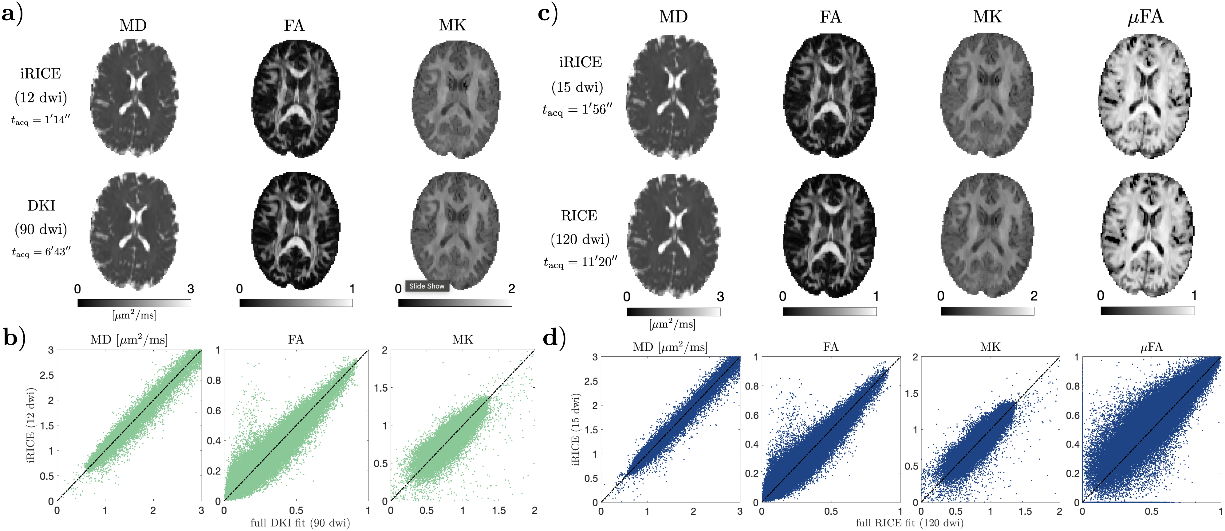
Figure S2: Comparison of iRICE (1-2 minutes) with fully sampled acquisitions (6-11 minutes) for magnitude-denoised data. (a,c): iRICE maps (top) vs fully sampled DKI maps (bottom) for a healthy volunteer. Panels (b) and (d) show scatter plots for all brain voxels in a normal volunteer.

References

- Callaghan [1991] P. T. Callaghan, Principles of Nuclear Magnetic Resonance Microscopy, Oxford Science Publications (Clarendon Press, 1991).
- Jones [2010] D. K. Jones, Diffusion MRI (Oxford University Press, 2010).
- Basser et al. [1994] P. J. Basser, J. Mattiello, and D. LeBihan, Estimation of the effective self-diffusion tensor from the NMR spin echo, Journal of Magnetic Resonance 103, 247 (1994).
- Jelescu and Budde [2017] I. O. Jelescu and M. D. Budde, Design and validation of diffusion MRI models of white matter, Frontiers in Physics 5, 61 (2017).
- Novikov et al. [2019] D. S. Novikov, E. Fieremans, S. N. Jespersen, and V. G. Kiselev, Quantifying brain microstructure with diffusion MRI: Theory and parameter estimation, NMR in Biomedicine , e3998 (2019).
- Alexander et al. [2019] D. C. Alexander, T. B. Dyrby, M. Nilsson, and H. Zhang, Imaging brain microstructure with diffusion MRI: practicality and applications, NMR in Biomedicine 32, e3841 (2019).
- Novikov [2021] D. S. Novikov, The present and the future of microstructure MRI: From a paradigm shift to normal science, Journal of Neuroscience Methods 351, 108947 (2021).
- Kiselev [2021] V. G. Kiselev, Microstructure with diffusion MRI: what scale we are sensitive to?, Journal of Neuroscience Methods 347, 108910 (2021).
- Weiskopf et al. [2021] N. Weiskopf, L. J. Edwards, G. Helms, S. Mohammadi, and E. Kirilina, Quantitative magnetic resonance imaging of brain anatomy and in vivo histology, Nature Reviews Physics 3, 570 (2021).
- Lampinen et al. [2023] B. Lampinen, F. Szczepankiewicz, J. Lätt, L. Knutsson, J. Mårtensson, I. M. Björkman-Burtscher, D. van Westen, P. C. Sundgren, F. Ståhlberg, and M. Nilsson, Probing brain tissue microstructure with mri: principles, challenges, and the role of multidimensional diffusion-relaxation encoding, NeuroImage 282, 120338 (2023).
- Assaf [2008] Y. Assaf, Can we use diffusion MRI as a bio-marker of neurodegenerative processes?, BioEssays 30, 1235 (2008).
- Nilsson et al. [2018] M. Nilsson, E. Englund, F. Szczepankiewicz, D. van Westen, and P. C. Sundgren, Imaging brain tumour microstructure, NeuroImage 182, 232 (2018), microstructural Imaging.
- van Kampen [1981] N. G. van Kampen, Stochastic Processes in Physics and Chemistry, 1st ed. (Elsevier, Oxford, 1981).
- Kiselev [2010] V. G. Kiselev, The cumulant expansion: an overarching mathematical framework for understanding diffusion NMR, in Diffusion MRI: Theory, Methods and Applications, edited by D. K. Jones (Oxford University Press, Oxford, 2010) Chap. 10, pp. 152–168.
- Westin et al. [2016] C.-F. Westin, H. Knutsson, O. Pasternak, F. Szczepankiewicz, E. Özarslan, D. van Westen, C. Mattisson, M. Bogren, L. J. O’Donnell, M. Kubicki, D. Topgaard, and M. Nilsson, q-space trajectory imaging for multidimensional diffusion MRI of the human brain, NeuroImage 135, 345 (2016).
- Novikov et al. [2014] D. S. Novikov, J. H. Jensen, J. A. Helpern, and E. Fieremans, Revealing mesoscopic structural universality with diffusion., Proceedings of the National Academy of Sciences of the United States of America 111, 5088 (2014).
- Kiselev [2017] V. G. Kiselev, Fundamentals of diffusion MRI physics, NMR in Biomedicine 30, 1 (2017).
- Cory et al. [1990] D. G. Cory, A. N. Garroway, and J. B. Miller, Applications of spin transport as a probe of local geometry, Polymer Preprints 31, 149 (1990).
- Mitra [1995] P. P. Mitra, Multiple wave-vector extensions of the NMR pulsed-field-gradient spin-echo diffusion measurement, Physical Review B 51, 15074 (1995).
- Mori and Van Zijl [1995] S. Mori and P. C. M. Van Zijl, Diffusion weighting by the trace of the diffusion tensor within a single scan, Magnetic Resonance in Medicine 33, 41 (1995).
- Shemesh et al. [2015] N. Shemesh, S. N. Jespersen, D. C. Alexander, Y. Cohen, I. Drobnjac, T. B. Dyrby, J. Finterbusch, M. A. Koch, T. Kuder, F. Laun, M. Lawrenz, H. Lundell, P. P. Mitra, M. Nilsson, E. Özarslan, D. Topgaard, and C.-F. Westin, Conventions and nomenclature for Double Diffusion Encoding NMR and MRI, Magnetic Resonance in Medicine 75, 82 (2015).
- Topgaard [2017] D. Topgaard, Multidimensional diffusion MRI, Journal of Magnetic Resonance 275, 98 (2017).
- Desmond-Hellmann [2012] S. Desmond-Hellmann, Toward precision medicine: A new social contract?, Science Translational Medicine 4, 129ed3 (2012).
- Kazhdan et al. [2003] M. Kazhdan, T. Funkhouser, and S. Rusinkiewicz, Rotation invariant spherical harmonic representation of 3d shape descriptors, in Proceedings of the 2003 Eurographics/ACM SIGGRAPH Symposium on Geometry Processing, SGP 03 (Eurographics Association, 2003) pp. 156–164.
- Gutman et al. [2007] B. Gutman, Y. Wang, L. M. Lui, T. F. Chan, and P. M. Thompson, Hippocampal surface discrimination via invariant descriptors of spherical conformals maps, in 2007 4th IEEE International Symposium on Biomedical Imaging: From Nano to Macro (2007) pp. 1316–1319.
- Mirzaalian et al. [2016] H. Mirzaalian, L. Ning, P. Savadjiev, O. Pasternak, S. Bouix, O. Michailovich, G. Grant, C. Marx, R. Morey, L. Flashman, M. George, T. McAllister, N. Andaluz, L. Shutter, R. Coimbra, R. Zafonte, M. Coleman, M. Kubicki, C. Westin, M. Stein, M. Shenton, and Y. Rathi, Inter-site and inter-scanner diffusion mri data harmonization, NeuroImage 135, 311 (2016).
- Reisert et al. [2017] M. Reisert, E. Kellner, B. Dhital, J. Hennig, and V. G. Kiselev, Disentangling micro from mesostructure by diffusion MRI: A Bayesian approach, NeuroImage 147, 964 (2017).
- Skibbe and Reisert [2017] H. Skibbe and M. Reisert, Spherical Tensor Algebra: A Toolkit for 3D Image Processing, Journal of Mathematical Imaging and Vision 58, 349 (2017).
- Novikov et al. [2018] D. S. Novikov, J. Veraart, I. O. Jelescu, and E. Fieremans, Rotationally-invariant mapping of scalar and orientational metrics of neuronal microstructure with diffusion MRI, NeuroImage 174, 518 (2018).
- Reisert et al. [2018] M. Reisert, V. A. Coenen, C. Kaller, K. Egger, and H. Skibbe, HAMLET: Hierarchical harmonic filters for learning tracts from diffusion mri (2018), arXiv:1807.01068 [cs.CV] .
- Smith et al. [2021] S. M. Smith, G. Douaud, W. Chen, T. Hanayik, F. Alfaro-Almagro, K. Sharp, and L. T. Elliott, An expanded set of genome-wide association studies of brain imaging phenotypes in UK Biobank, Nature Neuroscience 24, 737 (2021).
- Jack Jr. et al. [2008] C. R. Jack Jr., M. A. Bernstein, N. C. Fox, P. Thompson, G. Alexander, D. Harvey, B. Borowski, P. J. Britson, J. L. Whitwell, C. Ward, A. M. Dale, J. P. Felmlee, J. L. Gunter, D. L. Hill, R. Killiany, N. Schuff, S. Fox-Bosetti, C. Lin, C. Studholme, C. S. DeCarli, G. Krueger, H. A. Ward, G. J. Metzger, K. T. Scott, R. Mallozzi, D. Blezek, J. Levy, J. P. Debbins, A. S. Fleisher, M. Albert, R. Green, G. Bartzokis, G. Glover, J. Mugler, and M. W. Weiner, The alzheimer’s disease neuroimaging initiative (adni): Mri methods, Journal of Magnetic Resonance Imaging 27, 685 (2008).
- Jahanshad et al. [2013] N. Jahanshad, P. V. Kochunov, E. Sprooten, R. C. Mandl, T. E. Nichols, L. Almasy, J. Blangero, R. M. Brouwer, J. E. Curran, G. I. de Zubicaray, R. Duggirala, P. T. Fox, L. E. Hong, B. A. Landman, N. G. Martin, K. L. McMahon, S. E. Medland, B. D. Mitchell, R. L. Olvera, C. P. Peterson, J. M. Starr, J. E. Sussmann, A. W. Toga, J. M. Wardlaw, M. J. Wright, H. E. Hulshoff Pol, M. E. Bastin, A. M. McIntosh, I. J. Deary, P. M. Thompson, and D. C. Glahn, Multi-site genetic analysis of diffusion images and voxelwise heritability analysis: A pilot project of the enigma–dti working group, NeuroImage 81, 455 (2013).
- Glasser et al. [2016] M. F. Glasser, S. M. Smith, D. S. Marcus, J. L. R. Andersson, E. J. Auerbach, T. E. J. Behrens, T. S. Coalson, M. P. Harms, M. Jenkinson, S. Moeller, E. C. Robinson, S. N. Sotiropoulos, J. Xu, E. Yacoub, K. Ugurbil, and D. C. Van Essen, The human connectome project’s neuroimaging approach, Nature Neuroscience 19, 1175 (2016).
- Miller et al. [2016] K. L. Miller, F. Alfaro-Almagro, N. K. Bangerter, D. L. Thomas, E. Yacoub, J. Xu, A. J. Bartsch, S. Jbabdi, S. N. Sotiropoulos, J. L. R. Andersson, L. Griffanti, G. Douaud, T. W. Okell, P. Weale, I. Dragonu, S. Garratt, S. Hudson, R. Collins, M. Jenkinson, P. M. Matthews, and S. M. Smith, Multimodal population brain imaging in the UK Biobank prospective epidemiological study, Nature Neuroscience 19, 1523 (2016).
- Volkow et al. [2018] N. D. Volkow, G. F. Koob, R. T. Croyle, D. W. Bianchi, J. A. Gordon, W. J. Koroshetz, E. J. Perez-Stable, W. T. Riley, M. H. Bloch, K. Conway, B. G. Deeds, G. J. Dowling, S. Grant, K. D. Howlett, J. A. Matochik, G. D. Morgan, M. M. Murray, A. Noronha, C. Y. Spong, E. M. Wargo, K. R. Warren, and S. R. Weiss, The conception of the abcd study: From substance use to a broad nih collaboration, Developmental Cognitive Neuroscience 32, 4 (2018).
- Thorne [1980] K. S. Thorne, Multipole expansions of gravitational radiation, Rev. Mod. Phys. 52, 299 (1980).
- Tinkham [2003] M. Tinkham, Group Theory and Quantum Mechanics (Dover Books on Chemistry) (Dover Publications, 2003).
- Hall [2015] B. C. Hall, Lie Groups, Lie Algebras, and Representations (Springer, 2015).
- Stejskal and Tanner [1965] E. O. Stejskal and T. E. Tanner, Spin diffusion measurements: spin echoes in the presence of a time-dependent field gradient, The Journal of Chemical Physics 42, 288 (1965).
- Jensen et al. [2005] J. H. Jensen, J. A. Helpern, A. Ramani, H. Lu, and K. Kaczynski, Diffusional Kurtosis Imaging: The quantification of non-gaussian water diffusion by means of magnetic resonance imaging, Magnetic Resonance in Medicine 53, 1432 (2005).
- Itin and Hehl [2013] Y. Itin and F. W. Hehl, The constitutive tensor of linear elasticity: Its decompositions, cauchy relations, null lagrangians, and wave propagation, Journal of Mathematical Physics 54, 042903 (2013).
- Itin and Hehl [2015] Y. Itin and F. W. Hehl, Irreducible decompositions of the elasticity tensor under the linear and orthogonal groups and their physical consequences, in Journal of Physics: Conference Series, Vol. 597 (IOP Publishing, 2015) p. 012046.
- Eriksson et al. [2015] S. Eriksson, S. Lasic, M. Nilsson, C.-F. Westin, and D. Topgaard, NMR diffusion-encoding with axial symmetry and variable anisotropy: Distinguishing between prolate and oblate microscopic diffusion tensors with unknown orientation distribution, The Journal of Chemical Physics 142, 104201 (2015).
- Ghosh et al. [2012] A. Ghosh, T. Papadopoulo, and R. Deriche, Biomarkers for HARDI: 2nd & 4th order tensor invariants, in 2012 9th IEEE International Symposium on Biomedical Imaging (ISBI) (2012) pp. 26–29.
- Backus [1970] G. Backus, A geometrical picture of anisotropic elastic tensors, Reviews of Geophysics 8, 633 (1970).
- Betten [1987a] J. Betten, Irreducible invariants of fourth-order tensors, Mathematical Modelling 8, 29 (1987a).
- Betten [1987b] J. Betten, Invariants of fourth-order tensors, in Applications of tensor functions in solid mechanics, edited by J.-P. Boehler (Springer-Verlag, Vienna, Austria, 1987) Chap. 11, pp. 203–226.
- Bóna et al. [2004] A. Bóna, I. Bucataru, and M. Slawinski, Characterization of elasticity-tensor symmetries using su (2), Journal of Elasticity 75, 267 (2004).
- Moakher [2008] M. Moakher, Fourth-order cartesian tensors: old and new facts, notions and applications, The Quarterly Journal of Mechanics and Applied Mathematics 61, 181 (2008).
- Basser and Pajevic [2007] P. J. Basser and S. Pajevic, Spectral decomposition of a 4th-order covariance tensor: Applications to diffusion tensor MRI, Signal Processing 87, 220 (2007).
- Qi et al. [2009] L. Qi, D. Han, and E. X. Wu, Principal invariants and inherent parameters of diffusion kurtosis tensors, Journal of Mathematical Analysis and Applications 349, 165 (2009).
- Papadopoulo et al. [2014] T. Papadopoulo, A. Ghosh, and R. Deriche, Complete set of invariants of a 4thorder tensor: The 12 tasks of hardi from ternary quartics, in Medical Image Computing and Computer-Assisted Intervention – MICCAI 2014 (Springer International Publishing, Cham, 2014) pp. 233–240.
- Szczepankiewicz et al. [2016] F. Szczepankiewicz, D. van Westen, E. Englund, C.-F. Westin, F. Ståhlberg, J. Lätt, P. C. Sundgren, and M. Nilsson, The link between diffusion MRI and tumor heterogeneity: Mapping cell eccentricity and density by diffusional variance decomposition (DIVIDE), NeuroImage 142, 522 (2016).
- Lasič et al. [2014] S. Lasič, F. Szczepankiewicz, S. Eriksson, M. Nilsson, and D. Topgaard, Microanisotropy imaging: quantification of microscopic diffusion anisotropy and orientational order parameter by diffusion MRI with magic-angle spinning of the q-vector, Frontiers in Physics 2, 11 (2014).
- Hui et al. [2008] E. S. Hui, M. M. Cheung, L. Qi, and E. X. Wu, Towards better mr characterization of neural tissues using directional diffusion kurtosis analysis, NeuroImage 42, 122 (2008).
- Szczepankiewicz et al. [2019a] F. Szczepankiewicz, S. Hoge, and C.-F. Westin, Linear, planar and spherical tensor-valued diffusion mri data by free waveform encoding in healthy brain, water, oil and liquid crystals, Data in Brief 25, 104208 (2019a).
- Hansen et al. [2013] B. Hansen, T. E. Lund, R. Sangill, and S. N. Jespersen, Experimentally and computationally fast method for estimation of a mean kurtosis, Magnetic Resonance in Medicine 69, 1754 (2013).
- Nilsson et al. [2020] M. Nilsson, F. Szczepankiewicz, J. Brabec, M. Taylor, C.-F. Westin, A. Golby, D. van Westen, and P. C. Sundgren, Tensor-valued diffusion MRI in under 3 minutes: an initial survey of microscopic anisotropy and tissue heterogeneity in intracranial tumors, Magnetic Resonance in Medicine 83, 608 (2020).
- Ning et al. [2021] L. Ning, F. Szczepankiewicz, M. Nilsson, Y. Rathi, and C.-F. Westin, Probing tissue microstructure by diffusion skewness tensor imaging, Scientific Reports 135 (2021).
- Kiselev and Il’yasov [2007] V. G. Kiselev and K. A. Il’yasov, Is the “biexponential diffusion” biexponential?, Magnetic Resonance in Medicine 57, 464 (2007).
- Basser and Pajevic [2003] P. Basser and S. Pajevic, A normal distribution for tensor-valued random variables: applications to diffusion tensor MRI, IEEE Transactions on Medical Imaging 22, 785 (2003).
- Jian et al. [2007] B. Jian, B. C. Vemuri, E. Özarslan, P. R. Carney, and T. H. Mareci, A novel tensor distribution model for the diffusion-weighted mr signal, NeuroImage 37, 164 (2007).
- Glenn et al. [2015a] G. R. Glenn, J. A. Helpern, A. Tabesh, and J. H. Jensen, Quantitative assessment of diffusional kurtosis anisotropy, NMR in Biomedicine 28, 448 (2015a).
- Jespersen et al. [2007] S. N. Jespersen, C. D. Kroenke, L. Østergaard, J. J. H. Ackerman, and D. A. Yablonskiy, Modeling dendrite density from magnetic resonance diffusion measurements, NeuroImage 34, 1473 (2007).
- Jespersen et al. [2010] S. N. Jespersen, C. R. Bjarkam, J. R. Nyengaard, M. M. Chakravarty, B. Hansen, T. Vosegaard, L. Østergaard, D. Yablonskiy, N. C. Nielsen, and P. Vestergaard-Poulsen, Neurite density from magnetic resonance diffusion measurements at ultrahigh field: Comparison with light microscopy and electron microscopy, NeuroImage 49, 205 (2010).
- Fieremans et al. [2011] E. Fieremans, J. H. Jensen, and J. A. Helpern, White matter characterization with diffusional kurtosis imaging, NeuroImage 58, 177 (2011).
- Zhang et al. [2012] H. Zhang, T. Schneider, C. A. Wheeler-Kingshott, and D. C. Alexander, NODDI: Practical in vivo neurite orientation dispersion and density imaging of the human brain, NeuroImage 61, 1000 (2012).
- Sotiropoulos et al. [2012] S. N. Sotiropoulos, T. E. Behrens, and S. Jbabdi, Ball and rackets: Inferring fiber fanning from diffusion-weighted MRI, NeuroImage 60, 1412 (2012).
- Jensen et al. [2016] J. H. Jensen, G. Russell Glenn, and J. A. Helpern, Fiber ball imaging, NeuroImage 124, 824 (2016).
- Condon and Shortley [1964] E. U. Condon and G. H. Shortley, The theory of atomic spectra (The Cambridge University Press,, Cambridge, 1964.).
- Pozo et al. [2019] J. M. Pozo, S. Coelho, and A. F. Frangi, Tensorial formulation allowing to verify or falsify the microstructural standard model from multidimensional diffusion MRI, in Proceedings of the International Society of Magnetic Resonance in Medicine, Vol. 3560 (Wiley, 2019).
- Lu et al. [2006] H. Lu, J. Jensen, A. Ramani, and J. Helpern, Three-dimensional characterization of non-gaussian water diffusion in humans using diffusion kurtosis imaging, NMR in Biomedicine 19, 236 (2006).
- Jespersen et al. [2017] S. N. Jespersen, J. L. Olesen, B. Hansen, and N. Shemesh, Diffusion time dependence of microstructural parameters in fixed spinal cord, NeuroImage 182, 329 (2017).
- Glenn et al. [2015b] G. R. Glenn, J. A. Helpern, A. Tabesh, and J. H. Jensen, Quantitative assessment of diffusional kurtosis anisotropy, NMR in Biomedicine 28, 448 (2015b).
- Jespersen et al. [2013] S. N. Jespersen, H. Lundell, C. K. Sønderby, and T. B. Dyrby, Orientationally invariant metrics of apparent compartment eccentricity from double pulsed field gradient diffusion experiments, NMR in Biomedicine 26, 1647 (2013).
- Henriques et al. [2019] R. N. Henriques, S. N. Jespersen, and N. Shemesh, Microscopic anisotropy misestimation in spherical-mean single diffusion encoding MRI, Magnetic Resonance in Medicine 81, 3245 (2019).
- de Almeida Martins and Topgaard [2016] J. a. P. de Almeida Martins and D. Topgaard, Two-dimensional correlation of isotropic and directional diffusion using nmr, Phys. Rev. Lett. 116, 087601 (2016).
- Magdoom et al. [2021] K. N. Magdoom, S. Pajevic, G. Dario, and P. J. Basser, A new framework for mr diffusion tensor distribution, Scientific Reports 11, 2766 (2021).
- Seymour and Zaslavsky [1984] P. Seymour and T. Zaslavsky, Averaging sets: A generalization of mean values and spherical designs, Advances in Mathematics 52, 213 (1984).
- Szczepankiewicz et al. [2019b] F. Szczepankiewicz, C.-F. Westin, and M. Nilsson, Maxwell-compensated design of asymmetric gradient waveforms for tensor-valued diffusion encoding, Magnetic Resonance in Medicine 82, 1424 (2019b).
- Szczepankiewicz et al. [2019c] F. Szczepankiewicz, J. Sjölund, F. Ståhlberg, J. Lätt, and M. Nilsson, Tensor-valued diffusion encoding for diffusional variance decomposition (divide): Technical feasibility in clinical mri systems, PLOS ONE 14, 1 (2019c).
- Lemberskiy et al. [2019] G. Lemberskiy, S. Baete, J. Veraart, T. Shepherd, E. Fieremans, and D. S. Novikov, Achieving sub-mm clinical diffusion MRI resolution by removing noise during reconstruction using random matrix theory, In Proceedings 27th Scientific Meeting, 0770, International Society for Magnetic Resonance in Medicine, Montreal, Canada, 2019 (2019).
- Veraart et al. [2016] J. Veraart, E. Fieremans, and D. S. Novikov, Diffusion MRI noise mapping using random matrix theory, Magnetic Resonance in Medicine 76, 1582 (2016).
- Ades-Aron et al. [2018] B. Ades-Aron, J. Veraart, P. Kochunov, S. McGuire, P. Sherman, E. Kellner, D. S. Novikov, and E. Fieremans, Evaluation of the accuracy and precision of the diffusion parameter estimation with gibbs and noise removal pipeline, NeuroImage 183, 532 (2018).
- Lee et al. [2021] H.-H. Lee, D. S. Novikov, and E. Fieremans, Removal of partial fourier-induced gibbs (rpg) ringing artifacts in MRI, Magnetic Resonance in Medicine 86, 2733 (2021).
- Smith et al. [2004] S. M. Smith, M. Jenkinson, M. W Woolrich, C. F Beckmann, T. E J Behrens, H. Johansen-Berg, P. Bannister, M. Luca, I. Drobnjak, D. Flitney, R. Niazy, J. Saunders, J. Vickers, Y. Zhang, N. De Stefano, M. Brady, and P. Matthews, Advances in functional and structural mr image analysis and implementation as fsl, NeuroImage 23 Suppl 1, S208 (2004).
- Andersson et al. [2003] J. L. Andersson, S. Skare, and J. Ashburner, How to correct susceptibility distortions in spin-echo echo-planar images: application to diffusion tensor imaging, NeuroImage 20, 870 (2003).
- Wiest-Daesslé et al. [2007] N. Wiest-Daesslé, S. Prima, P. Coupé, S. P. Morrissey, and C. Barillot, Non-local means variants for denoising of diffusion-weighted and diffusion tensor MRI, in Medical Image Computing and Computer-Assisted Intervention (MICCAI), Vol. 10 (Springer, 2007) pp. 344—351.
- Veraart et al. [2013] J. Veraart, J. Sijbers, S. Sunaert, A. Leemans, and B. Jeurissen, Weighted linear least squares estimation of diffusion MRI parameters: Strengths, limitations, and pitfalls, NeuroImage 81, 335 (2013).
- Herberthson et al. [2021] M. Herberthson, D. Boito, T. D. Haije, A. Feragen, C.-F. Westin, and E. Özarslan, Q-space trajectory imaging with positivity constraints (QTI+), NeuroImage 238, 118198 (2021).