Cosmological constraints on anisotropic Thurston geometries

Abstract

Much of modern cosmology relies on the Cosmological Principle, the assumption that the Universe is isotropic and homogeneous on sufficiently large scales, but it remains worthwhile to examine cosmological models that violate this principle slightly. We examine a class of such spacetimes that maintain homogeneity but break isotropy through their underlying local spatial geometries. These spacetimes are endowed with one of five anisotropic model geometries of Thurston’s geometrization theorem, and their evolution is sourced with perfect fluid dust and cosmological constant. We show that the background evolution of these spacetimes induces fluctuations in the observed cosmic microwave background (CMB) temperature with amplitudes coupled to the curvature parameter $\Omega_{K}$. In order for these fluctuations to be compatible with the observed CMB angular power spectrum, we find $|\Omega_{K}|\lesssim 10^{-5}$ is required in all five geometries, with two geometries requiring $|\Omega_{K}|\lesssim 10^{-10}$. This strongly limits the cosmological consequences of these models.

1 Introduction

One of the main assumptions made in the current standard model of cosmology, $\Lambda$CDM, is that the Universe is spatially homogeneous and isotropic on large enough scales. Known as the Cosmological Principle, this assumption restricts the large-scale geometry of the Universe to one of three types, which can be presented simultaneously in a Friedmann-Lemaître-Robertson-Walker (FLRW) metric. Though the Cosmological Principle is well-corroborated by large-scale structure and other cosmological observables, hints of this postulate being violated have emerged in recent decades.

Among the strongest pieces of evidence for the Cosmological Principle has been the high degree of isotropy of the blackbody temperature of the cosmic microwave background (CMB) radiation, first reported by Penzias and Wilson [1]. More recently, the isotropy of the statistical properties of the very small amplitude fluctuations in the temperature and polarization of the CMB has been tested [2, 3], and several violations of isotropy have been reported. In particular, a handful of large-angle features in the observed CMB temperature [4] were discovered in the first WMAP data release [5] and were suggested to indicate significant deviation from statistical isotropy. These features have come to be known as the “large-angle anomalies,” and their significance has persisted in subsequent Planck datasets [6], with recent work arguing these anomalies jointly constitute a $>5\sigma$ violation of statistical isotropy [7].

This collection of evidence warrants consideration of cosmological models that deviate slightly from the Cosmological Principle, in particular by violating spatial isotropy. In this work, we investigate the consequences of breaking spatial isotropy through geometry – i.e., by equipping the Universe with a background metric that is homogeneous but anisotropic. Relaxing the requirement of isotropy allows the large-scale geometry of the Universe to be of a slightly more general class than the three FLRW geometries.

Historically, work on the cosmology of anisotropic spaces has centered around the Bianchi models (see [8] for review). These are 3+1 spacetimes whose homogeneous spatial part corresponds to a 3-dimensional real Lie algebra, falling into one of eleven types within a classification devised by Bianchi in 1898 [9]. A subset of the Bianchi models have been invoked as potential explanations of CMB anomalies [10, 11], but their deviation from isotropy is strongly constrained. This is because many Bianchi spaces require anisotropic expansion – i.e., multiple scale factors – if they are sourced by perfect fluid stress energies. This anisotropic expansion leaves potentially detectable imprints on cosmological observables, often characterized by the resulting “shear.” For instance, in the subset of Bianchi spaces that explicitly contain the three FLRW metrics as special cases, anisotropic expansion is strongly constrained by the anisotropies it induces in the CMB temperature [12, 13]. Constraints have also been derived from the imprint of shear on nucleosynthesis [14].

This work considers a more recently developed class of homogeneous but not necessarily isotropic geometries known as the Thurston geometries. These eight model geometries exhaust the possible local geometries of closed homogeneous 3-manifolds according to Thurston’s geometrization theorem [15]. Thurston’s classification schema is analogous to Bianchi’s, and all but one of the Thurston geometries fall within a Bianchi group [16]. Out of the eight Thurston geometries, three are the open, closed, and flat FLRW geometries, and the remaining five are anisotropic. These latter subset of spaces remain largely unconstrained within a cosmological context (although see [17, 18]).

The dynamics and distance measures of spacetimes with Thurston geometries as spatial parts, which we will dub Thurston spacetimes, have recently been investigated [18], albeit when equipped with a single scale factor. This requires invoking an anisotropic fluid fine-tuned to prohibit anisotropic expansion. The evolution of scale factors under isotropic dust and cosmological constant is provided for each Thurston spacetime in [18], but no accompanying constraints on curvature scales are derived.

In this paper, we provide strong constraints on the curvature of all five anisotropic Thurston spacetimes for the first time. After providing representations of each anisotropic Thurston geometry in Section 2, we review the dynamics of the corresponding spacetimes under the presence of perfect fluid dust and cosmological constant in Section 3, where we find anisotropic expansion is required. Consequently, when coupled with underlying geometric anisotropy, we find that the local flux of CMB photons is distorted, and a present-day observer interprets this flux as that of a blackbody with a non-uniform temperature. The amplitudes of the CMB temperature fluctuations induced in these geometries are coupled to the curvature parameter $\Omega_{K}$, which is therefore strongly constrained by the isotropy of the CMB. We derive this constraint for each of the five anisotropic Thurston spacetimes in Sections 4–6, finding that $|\Omega_{K}|\lesssim 10^{-5}$ in all five geometries, with two even requiring $|\Omega_{K}|\lesssim 10^{-10}$.

The GitHub repository associated with this study is publicly available at https://github.com/cwru-pat/ThurstonGeometry. Codes will be deposited there as publicly usable versions become available.

2 Thurston geometries

In 1982 Thurston conjectured [15] (and Perelman later proved [19, 20])

The interior of every compact 3-manifold has a canonical decomposition into pieces which have geometric structures.

In practice, this reduces to a set of eight local three-geometries – three being the well-known and well-studied isotropic FLRW geometries: flat ($\mathbb{R}^{3}$), spherical ($S^{3}$), and hyperbolic ($\mathbb{H}^{3}$). The remaining five anisotropic local three-geometries are less well-known and will be discussed below. Though the conjecture allows for a decomposition of the full space, in this work we restrict to the case where the observable Universe has just one of these eight local geometries. Without loss of generality, we take the topology to be the covering space of that geometry. We refer curious readers to the growing body of work on detecting nontrivial topology in the Universe, e.g., [21].

In the remainder of this section, we present metrics for each of the five anisotropic Thurston geometries. We adopt the representations of [18], where the parameter $\kappa$ found in the spatial part of each metric distinguishes between positive ($\kappa>0$) and negative ($\kappa<0$) spatial curvature. All of these local geometries can be made arbitrarily close to flat space in some finite neighborhood by taking $\kappa$ sufficiently close to zero.

2.1 $S^{2}\times\mathbb{R}$ and $\mathbb{H}^{2}\times\mathbb{R}$

The first two anisotropic geometries in Thurston’s classification system are $S^{2}\times\mathbb{R}$ and $\mathbb{H}^{2}\times\mathbb{R}$. In the literature, spacetimes equipped with $S^{2}\times\mathbb{R}$ spatial geometries are often referred to as Kantowski-Sachs spaces [22], and $\mathbb{H}^{2}\times\mathbb{R}$ falls under type III of the Bianchi classification.

$S^{2}\times\mathbb{R}$ and $\mathbb{H}^{2}\times\mathbb{R}$ are the most straightforward to understand among the five geometries we are considering: $S^{2}\times\mathbb{R}$ admits positive curvature ($\kappa>0$) along two spatial directions and zero curvature along one, while $\mathbb{H}^{2}\times\mathbb{R}$ is analogous but with its curved directions having negative curvature ($\kappa<0$). This description leads naturally to a spatial metric separated into a hyperspherical part and a flat part:

$$\mathrm{d}\Sigma_{3}^{2}=\mathrm{d}\chi^{2}+S_{\kappa}(\chi)^{2}\mathrm{d}\varphi^{2}+\mathrm{d}z^{2},$$ (2.1)

where $\chi\in[0,\infty)$, $\varphi\in[0,2\pi)$, $z\in\mathbb{R}$, and

$$S_{\kappa}(\chi)=\begin{cases}\sin(\chi\sqrt{\kappa})/\sqrt{\kappa},&\kappa>0,\\ \sinh(\chi\sqrt{-\kappa})/\sqrt{-\kappa},&\kappa<0.\end{cases}$$ (2.2)

2.2 $\widetilde{U(\mathbb{H}^{2})}$

The next anisotropic Thurston geometry is $\widetilde{U(\mathbb{H}^{2})}$, the universal cover of $U(\mathbb{H}^{2})$, the unit tangent bundle of the hyperbolic plane, and falls within Bianchi types III and VIII. We adopt the spatial metric derived in [16],

$$\mathrm{d}\Sigma_{3}^{2}=\mathrm{d}x^{2}+\cosh(2x\sqrt{-\kappa})\mathrm{d}y^{2}+\mathrm{d}z^{2}+2\sinh(x\sqrt{-\kappa})\mathrm{d}y\mathrm{d}z,$$ (2.3)

where $\kappa<0$ and $x,y,z\in\mathbb{R}$.

This geometry is often referred to as $\widetilde{\text{SL}(2,\mathbb{R})}$ in the literature since this space is diffeomorphic to $\widetilde{U(\mathbb{H}^{2})}$. However, these two spaces are not isomorphic so they are not interchangeable in a physical context.

2.3 Nil

The next anisotropic Thurston geometry is Nil, the geometry of the Heisenberg group. It can be thought of as twisted $E^{2}\times\mathbb{R}$ and falls within Bianchi type II. It can be represented with the spatial metric

$$\mathrm{d}\Sigma_{3}^{2}=\mathrm{d}x^{2}+(1+\kappa x^{2})\mathrm{d}y^{2}+\mathrm{d}z^{2}-2x\sqrt{-\kappa}\mathrm{d}y\mathrm{d}z,$$ (2.4)

where $x,y,z\in\mathbb{R}$.

2.4 Solv

The final anisotropic Thurston geometry is Solv, the geometry of solvable Lie groups. The Solv geometry falls within Bianchi type VI₀, and can be represented with the spatial metric

$$\mathrm{d}\Sigma_{3}^{2}=\mathrm{e}^{2z\sqrt{-\kappa}}\mathrm{d}x^{2}+\mathrm{e}^{-2z\sqrt{-\kappa}}\mathrm{d}y^{2}+\mathrm{d}z^{2},$$ (2.5)

where $x,y,z\in\mathbb{R}$.

3 Evolution of anisotropic Thurston spacetimes

According to general relativity, the evolution of any spacetime is governed by the stress energy content of the universe through Einstein’s field equations

$$\tensor{G}{{}^{\mu}_{\nu}}=8\pi G\tensor{T}{{}^{\mu}_{\nu}},$$ (3.1)

where our choice of $c=1$ units persists in all subsequent calculations. Thus the evolution of spacetimes with anisotropic Thurston spatial geometries is sensitive to the choice of stress energy. For example, it is possible to equip an anisotropic spacetime with a single scale factor, say $a(t)$, in what are commonly referred to as “shear-free” models in the literature [23, 24]. The stress energy tensor characteristic of the fluid required to achieve this scales like $a^{-2}$ and contains off-diagonal elements that are chosen precisely to prevent anisotropic expansion. The fine-tuning required for this cancellation to occur makes this approach less compelling from a theoretical perspective and requires the introduction of non-standard sources of stress energy.

Following [18], in this work we take the opposite approach of using known sources of isotropic stress energy and allowing anisotropic expansion. Here our isotropic stress energy contains perfect fluids in the form of dust (pressureless with energy density $\rho$) and a cosmological constant (with $\Lambda=8\pi G\rho_{\Lambda}$ and $p_{\Lambda}=-\rho_{\Lambda}$). With this content the stress-energy tensor takes the form

$$\tensor{T}{{}^{\mu}_{\nu}}=\rho u^{\mu}u_{\nu}-\frac{\Lambda}{8\pi G}\tensor{\delta}{{}^{\mu}_{\nu}},$$ (3.2)

where $u^{\mu}$ is the 4-velocity of the fluid. Working in the co-moving frame where $u^{\mu}=(1,0,0,0)$ yields the diagonal stress energy tensor commonly studied in $\Lambda$CDM cosmology

$$\tensor{T}{{}^{\mu}_{\nu}}=\operatorname{diag}\!\left(-\rho-\frac{\Lambda}{8\pi G},-\frac{\Lambda}{8\pi G},-\frac{\Lambda}{8\pi G},-\frac{\Lambda}{8\pi G}\right).$$ (3.3)

In general, the spatial metric of the Thurston geometries has the form

$$\mathrm{d}\Sigma_{3}^{2}=\gamma_{ij}\mathrm{d}x^{i}\mathrm{d}x^{j},$$ (3.4)

so that the spacetime metric is given by

$$\mathrm{d}s^{2}=-\mathrm{d}t^{2}+\gamma_{k\ell}\tensor{\alpha}{{}^{k}_{i}}\tensor{\alpha}{{}^{\ell}_{j}}\mathrm{d}x^{i}\mathrm{d}x^{j},$$ (3.5)

where we allow for (potentially independent) scale factors through the diagonal matrix

$$\tensor{\alpha}{{}^{k}_{i}}=\operatorname{diag}(a_{1}(t),a_{2}(t),a_{3}(t))\indices{{}^{k}_{i}}.$$ (3.6)

With anisotropic expansion introduced, the Einstein field equations for the stress energy tensor (3.3) are quite similar among the five anisotropic Thurston geometries. The diagonal elements of their Einstein field equations all have the form

$$\indices{{}^{0}_{0}} :\qquad\frac{\dot{a}_{1}\dot{a}_{2}}{a_{1}a_{2}} +\frac{\dot{a}_{2}\dot{a}_{3}}{a_{2}a_{3}} +\frac{\dot{a}_{3}\dot{a}_{1}}{a_{3}a_{1}} +\tensor{\Delta}{{}^{0}_{0}} {}=~{} \Lambda+\frac{k^{(0)}\kappa}{a_{\mathrm{dom}}^{2}}+8\pi G\rho,$$

$$\indices{{}^{1}_{1}} :\qquad\frac{\ddot{a}_{2}}{a_{2}} +\frac{\ddot{a}_{3}}{a_{3}} +\frac{\dot{a}_{2}\dot{a}_{3}}{a_{2}a_{3}} +\tensor{\Delta}{{}^{1}_{1}} {}=~{} \Lambda+\frac{k^{(1)}\kappa}{a_{\mathrm{dom}}^{2}},$$ (3.7)

$$\indices{{}^{2}_{2}} :\qquad\frac{\ddot{a}_{3}}{a_{3}} +\frac{\ddot{a}_{1}}{a_{1}} +\frac{\dot{a}_{3}\dot{a}_{1}}{a_{3}a_{1}} +\tensor{\Delta}{{}^{2}_{2}} {}=~{} \Lambda+\frac{k^{(2)}\kappa}{a_{\mathrm{dom}}^{2}},$$

$$\indices{{}^{3}_{3}} :\qquad\frac{\ddot{a}_{1}}{a_{1}} +\frac{\ddot{a_{2}}}{a_{2}} +\frac{\dot{a}_{1}\dot{a}_{2}}{a_{1}a_{2}} +\tensor{\Delta}{{}^{3}_{3}} {}=~{} \Lambda+\frac{k^{(3)}\kappa}{a_{\mathrm{dom}}^{2}}.$$

The dependence of (3) on the choice of geometry lies in the term proportional to $\kappa$, where the constants $k^{(\mu)}$ and accompanying scale factor $a_{\mathrm{dom}}$ are listed in Table 1, and in extra contributions $\tensor{\Delta}{{}^{\mu}_{\nu}}$ to the Einstein tensor. We define $\tensor{\Delta}{{}^{\mu}_{\nu}}$ to include all of the off-diagonal elements of the Einstein tensor, meaning the accompanying off-diagonal field equations are, given our insistence on a diagonal stress-energy tensor, simply

$$\tensor{\Delta}{{}^{\mu}_{\nu}}=0.$$ (3.8)

Geometry	$k^{(0)}$	$k^{(1)}$	$k^{(2)}$	$k^{(3)}$	$a_{\mathrm{dom}}$
$S^{2}\times\mathbb{R}$ and $\mathbb{H}^{2}\times\mathbb{R}$	-1	0	0	-1	$a_{1}\equiv a$
$\widetilde{U(\mathbb{H}^{2})}$	-5/4	1/4	1/4	-7/4	$a_{1}\equiv a$
Nil	-1/4	1/4	1/4	-3/4	$a_{1}\equiv a$
Solv	-1	-1	-1	1	$a_{3}\equiv b$

Table 1: Curvature coupling constants $k^{(i)}$ and the scale factor in the curvature term $a_{\mathrm{dom}}$ for each of the five anisotropic Thurston spacetimes.

The evolution of the scale factors are constrained by (3.8), since the off-diagonal elements of $\tensor{\Delta}{{}^{\mu}_{\nu}}$ will not necessarily be zero if all of the scale factors evolve independently. We will show that the solutions to the diagonal field equations (3) equate certain pairs of scale factors in a way that satisfies (3.8) in the limit that the spatial curvature is small, which is mandated by the Universe being approximately flat on large scales. To this end, we may define an average scale factor as the geometric mean

$$A(t)\equiv\left[a_{1}(t)a_{2}(t)a_{3}(t)\right]^{1/3},$$ (3.9)

the Hubble parameter associated with it

$$H(t)\equiv\frac{\dot{A}}{A}=\frac{1}{3}\left(\frac{\dot{a}_{1}}{a_{1}}+\frac{\dot{a}_{2}}{a_{2}}+\frac{\dot{a}_{3}}{a_{3}}\right),$$ (3.10)

and the dimensionless curvature fraction

$$\Omega_{K}\equiv\frac{k^{(0)}\kappa}{3H_{0}^{2}},$$ (3.11)

where $H_{0}\equiv H(t_{0})$ is the current ($t=t_{0}$) value of the Hubble expansion parameter. More precisely, then, the small curvature limit corresponds to $|\Omega_{K}|\ll 1$, ensuring the terms proportional to $\kappa$ on the right-hand side of (3) are subdominant.

With this, taking linear combinations of the spatial equations in Section 3, and following [18] we can expand the individual scale factors in powers $\Omega_{K}$ to find

$$a_{i}(t)=A(t)\left[1+\Omega_{K}K^{(i)}F(t)+\mathcal{O}(\Omega_{K}^{2})\right],$$ (3.12)

where

$$K^{(1)} \equiv\frac{k^{(2)}+k^{(3)}-2k^{(1)}}{k^{(0)}},$$

$$K^{(2)} \equiv\frac{k^{(3)}+k^{(1)}-2k^{(2)}}{k^{(0)}},$$ (3.13)

$$K^{(3)} \equiv\frac{k^{(1)}+k^{(2)}-2k^{(3)}}{k^{(0)}}$$

are given in Table 2 and

$$F[A(t)]\equiv\frac{2}{5\Omega_{m}}\int_{A(t_{0})}^{A(t)}\,\frac{\tensor[_{2}]{F}{{}_{1}}\!\left(\frac{1}{2},\frac{5}{6};\frac{11}{6};-a^{\prime 3}\frac{\Omega_{\Lambda}}{\Omega_{m}}\right)}{\sqrt{1+a^{\prime 3}\frac{\Omega_{\Lambda}}{\Omega_{m}}}}\,\mathrm{d}a^{\prime}\,.$$ (3.14)

Here $\tensor[_{2}]{F}{{}_{1}}$ is the hypergeometric function, the integral is from the time $t_{0}$, and we have made the standard definitions

$$\Omega_{m}\equiv\frac{8\pi G\rho(t_{0})}{3H_{0}^{2}}\,\mbox{ and }\Omega_{\Lambda}\equiv\frac{\Lambda}{3H_{0}^{2}}.$$ (3.15)

Geometry	$K^{(1)}$	$K^{(2)}$	$K^{(3)}$
$S^{2}\times\mathbb{R}$ and $\mathbb{H}^{2}\times\mathbb{R}$	$\hphantom{-}1$	$\hphantom{-}1$	$-2$
$\widetilde{U(\mathbb{H}^{2})}$	$\hphantom{-}8/5$	$\hphantom{-}8/5$	$-16/5$
Nil	$\hphantom{-}4$	$\hphantom{-}4$	$-8$
Solv	$-2$	$-2$	$\hphantom{-}4$

Table 2: Curvature coupling differences $K^{(i)}$ as defined in (3) for the five anisotropic Thurston spacetimes.

While these same solutions were obtained in [18] and we have followed a similar procedure, there is an important difference. Namely, in that work, $\tensor{\Delta}{{}^{\mu}_{\nu}}$ was set to zero by equating scale factors as necessary in each geometry before solving the field equations. In $\widetilde{U(\mathbb{H}^{2})}$ and Nil, this meant imposing the restriction $a_{1}=a_{2}=a_{3}$ and $a_{2}=a_{3}$, respectively. However, this is inconsistent with (3.12) given the values of $K^{(i)}$ in Table 2 which indicates that $a_{1}=a_{2}\neq a_{3}$ to order $\Omega_{K}$ in all geometries. To avoid this contradiction we instead use (3.12) along with the $K^{(i)}$ from Table 2 to determine which scale factors to equate. With these solutions, we find that $\tensor{\Delta}{{}^{\mu}_{\nu}}$ still vanishes to order $\Omega_{K}$ across all geometries. In $S^{2}\times\mathbb{R}$, $\mathbb{H}^{2}\times\mathbb{R}$, and Solv, this is because the only non-trivial entries of $\tensor{\Delta}{{}^{\mu}_{\nu}}$ exhibit the proportionality

$$\tensor{\Delta}{{}^{0}_{1}}=-a_{1}^{2}\tensor{\Delta}{{}^{1}_{0}}\propto\left(\frac{\dot{a_{1}}}{a_{1}}-\frac{\dot{a_{2}}}{a_{2}}\right),$$ (3.16)

which vanishes by the equivalence of $a_{1}$ and $a_{2}$ to this order. In the remaining two geometries, $\widetilde{U(\mathbb{H}^{2})}$ and Nil, the entries of $\tensor{\Delta}{{}^{\mu}_{\nu}}$ are less obviously zero to working order and take the form

$$\tensor{\Delta}{{}^{\mu}_{\nu}}=\sqrt{\Omega_{K}}f(a,b)\,.$$ (3.17)

Here $f(a,b)$ contains differences of scale factors $a_{1}=a_{2}\equiv a$ and $a_{3}\equiv b$. Thus $f$ must be at least $\mathcal{O}(\sqrt{\Omega_{K}})$ since it must disappear in the flat limit, i.e., when $\Omega_{K}\to 0$. In practice $f$ is found to be $\mathcal{O}(\Omega_{K})$ as shown in Appendix A, where more detailed expressions for (3.17) are listed. We proceed knowing that we may neglect $\tensor{\Delta}{{}^{\mu}_{\nu}}$ to working order in $\Omega_{K}$.

Turning to the evolution of the average scale factor $A(t)$, we may square Eq. 3.10 to find

$$H^{2}=\frac{1}{9}\sum_{i=1}^{3}\left(\frac{\dot{a}_{i}}{a_{i}}\right)^{2}+\frac{2}{9}\left(\Lambda+\frac{k^{(0)}\kappa}{a_{\mathrm{dom}}^{2}}+8\pi G\rho\right),$$ (3.18)

where we have used $\tensor{\Delta}{{}^{\mu}_{\nu}}=0$ to the required order and have used the ${}^{0}\text{}_{0}$ equation from (3) to simplify the second term. It follows from (3.12) that

$$\sum_{i=1}^{3}\left(\frac{\dot{a}_{i}}{a_{i}}\right)^{2}=3H^{2}+\Omega_{K}q(t)\sum_{i}K^{(i)}+\mathcal{O}(\Omega_{K}^{2}).$$ (3.19)

for a known function $q(t)$. The form of $q(t)$ is unimportant since from (3)

$$\sum_{i=1}^{3}K^{(i)}=0\,,$$ (3.20)

independent of geometry. Combining (3.18) and (3.19), we obtain the Friedmann equation

$$H^{2}=\left(\frac{\dot{A}}{A}\right)^{2}=H_{0}^{2}\left(\frac{\Omega_{m}}{A^{3}}+\Omega_{\Lambda}+\frac{\Omega_{K}}{A^{2}}\right)+\mathcal{O}(\Omega_{K}^{2}).$$ (3.21)

Expanding in powers of $\Omega_{K}$

$$A(t)=A^{(0)}(t)+\Omega_{K}A^{(1)}(t)+\mathcal{O}(\Omega_{K}^{2}),$$ (3.22)

and substituting into (3.21) we find the desired evolution. As expected, the zeroth order term is the FLRW expansion factor for a matter and cosmological-constant-dominated universe

$$A^{(0)}(t)=\left(\frac{\Omega_{m}}{\Omega_{\Lambda}}\right)^{1/3}\sinh^{2/3}\!\left(\frac{3\sqrt{\Omega_{\Lambda}}}{2}H_{0}t\right).$$ (3.23)

We can also obtain an explicit form for $A^{(1)}(t)$, however, it will not be needed in subsequent calculations. Finally, combining these results with Eq. 3.12 we arrive at the fully expanded time evolution for the scale factors

$$a_{i}(t)=A^{(0)}(t)+\Omega_{K}\left[A^{(1)}(t)+K^{(i)}A^{(0)}(t)F(A^{(0)}(t))\right]+\mathcal{O}(\Omega_{K}^{2}).$$ (3.24)

We have thus demonstrated that homogeneous spacetimes with anisotropic Thurston geometries are able to evolve under a perfect fluid stress energy to $\mathcal{O}(\Omega_{K})$ when multiple scale factors are introduced. The expansion, combined with geometric anisotropy, induces angular dependence in cosmological observables and distance measures. In particular, a completely isotropic CMB at last scattering will be observed to be anisotropic by a post-last-scattering observer, such as ourselves. In the following sections, we show that these fluctuations allow us to put strong bounds on $\Omega_{K}$ should our Universe possess these geometries.

4 $S^{2}\times\mathbb{R}$ and $\mathbb{H}^{2}\times\mathbb{R}$

We begin by constraining the curvature in spacetimes with $S^{2}\times\mathbb{R}$ and $\mathbb{H}^{2}\times\mathbb{R}$ spatial geometries, which have the metric

$$\mathrm{d}s^{2}=-\mathrm{d}t^{2}+a(t)^{2}\left[\mathrm{d}\chi^{2}+S^{2}_{\kappa}(\chi)\mathrm{d}\varphi^{2}\right]+b(t)^{2}\mathrm{d}z^{2},$$ (4.1)

where we use the identification $a_{1}(t)=a_{2}(t)\equiv a(t)$ and $a_{3}(t)\equiv b(t)$ in each geometry found in Section 3.

Recall for $\mathbb{H}^{2}\times\mathbb{R}$ that

$$S_{\kappa}(\chi)=\frac{\sinh(\sqrt{-\kappa}\chi)}{-\kappa}.$$ (4.2)

Since $\kappa$ has dimensions of inverse length squared, to expand the metric we require $\sqrt{-\kappa}\chi\ll 1$. Recalling (3.11) we have

$$\sqrt{-\kappa}\chi=\sqrt{3\Omega_{K}}H_{0}\chi\ll 1.$$ (4.3)

To simplify notation here and throughout we will write all distances in units of $H_{0}^{-1}$. With this, for $S^{2}\times\mathbb{R}$ and $\mathbb{H}^{2}\times\mathbb{R}$ we have

$$S_{\kappa}(\chi)=\begin{cases}\sin(\sqrt{-3\Omega_{K}}\chi)/\sqrt{-3\Omega_{K}},&\Omega_{K}<0,\\ \sinh(\sqrt{3\Omega_{K}}\chi)/\sqrt{3\Omega_{K}},&\Omega_{K}>0.\end{cases}$$ (4.4)

The photons emitted during recombination travel along null geodesics of the spacetime, which we compute in Section 4.1. These trajectories are warped by anisotropic curvature and spatial expansion, meaning that the local photon fluxes at recombination and today computed in Section 4.2 are different. A present-day observer interprets this photon flux as that of a blackbody with a temperature that is a function of solid angle in the sky, which we confront against the observed CMB angular power spectrum to derive bounds on $\Omega_{K}$ in Section 4.3.

4.1 Null geodesics

We start by computing the trajectories $x^{\mu}(\lambda)=\left(t(\lambda),\chi(\lambda),\varphi(\lambda),z(\lambda)\right)$, parameterized by the affine parameter $\lambda$, of photons emitted at recombination that are later detected by an observer at the present time $t(\lambda_{0})=t_{0}$ located at the origin of our coordinate system. Such trajectories obey the geodesic equation

$$\frac{\mathrm{d}^{2}x^{\mu}}{\mathrm{d}\lambda^{2}}+\Gamma^{\mu}_{\alpha\beta}\frac{\mathrm{d}x^{\alpha}}{\mathrm{d}\lambda}\frac{\mathrm{d}x^{\beta}}{\mathrm{d}\lambda}=0.$$ (4.5)

Much like spherical symmetry allows us to impose that CMB photons follow purely radial geodesics in FLRW spaces, rotational symmetry within the $(\chi,\varphi)$-plane in $S^{2}\times\mathbb{R}$ and $\mathbb{H}^{2}\times\mathbb{R}$ allows us to set $\mathrm{d}\varphi/\mathrm{d}\lambda\equiv\varphi^{\prime}(\lambda)=0$. Upon doing this, the geodesic equations for the remaining spatial coordinates read

$$\chi^{\prime\prime}+\frac{2a^{\prime}}{a}\chi^{\prime}=\frac{1}{a^{2}}\frac{\mathrm{d}}{\mathrm{d}\lambda}\!\left(a^{2}\chi^{\prime}\right) =0,$$

$$z^{\prime\prime}+\frac{2b^{\prime}}{b}z^{\prime}=\frac{1}{b^{2}}\frac{\mathrm{d}}{\mathrm{d}\lambda}\!\left(b^{2}z^{\prime}\right) =0,$$ (4.6)

which of course are solved by

$$\chi^{\prime}(\lambda)=\frac{c_{\chi}}{a(t(\lambda))^{2}}$$

$$z^{\prime}(\lambda)=\frac{c_{z}}{b(t(\lambda))^{2}}$$ (4.7)

where $c_{\chi}$ and $c_{z}$ are constants. By demanding the geodesics obey the null condition

$$g_{\alpha\beta}\frac{\mathrm{d}x^{\alpha}}{\mathrm{d}\lambda}\frac{\mathrm{d}x^{\beta}}{\mathrm{d}\lambda}=0,$$ (4.8)

one recovers the first order equation

$$t^{\prime 2}=(a\chi^{\prime})^{2}+(bz^{\prime})^{2},$$ (4.9)

which can in principle be solved for $t(\lambda)$. However, this derivative expression is sufficient for the subsequent analysis based on the 4-velocities of incoming photons.

4.2 CMB photon flux

With knowledge of these geodesics, we turn our attention to the distortions induced in the CMB. To do this, we first examine the local flux of CMB photons propagating through a point in space at the time of recombination, i.e., on the last scattering surface,

$$\Phi(E_{r})=\frac{\mathrm{d}N_{r}(E_{r})}{\mathrm{d}\Omega_{r}\mathrm{d}A_{r}\mathrm{d}t_{r}\mathrm{d}E_{r}},$$ (4.10)

where $\mathrm{d}N_{r}(E_{r})$ is the number of photons with energies between $E_{r}$ and $E_{r}+\mathrm{d}E_{r}$ received within a solid angle $\mathrm{d}\Omega_{r}=\mathrm{d}(\cos\theta_{r})\mathrm{d}\varphi_{r}$ in an area $\mathrm{d}A_{r}$ during a time $\mathrm{d}t_{r}$. As these photons propagate from the last scattering surface through an expanding anisotropic geometry, they experience a redshift that will be a function of their direction of propagation, and thus as a function of the direction on the sky from which an observer receives them. The flux of CMB photons observed today will differ from that present at recombination due to this effect. In particular, an isotropic flux at recombination will be observed today as anisotropic. This present-day flux can be obtained by performing a change of coordinates from $A_{r}$, $t_{r}$, and $E_{r}$ at recombination to $A_{0}$, $t_{0}$, and $E_{0}$, today. The effect on the flux is captured through the appropriate Jacobian factor, which simplifies to

$$\Phi(E_{0})=\Phi(E_{r})\left(\frac{\mathrm{d}\Omega_{r}}{\mathrm{d}\Omega_{0}}\right)\left(\frac{\mathrm{d}A_{r}\mathrm{d}t_{r}}{\mathrm{d}A_{0}\mathrm{d}t_{0}}\right)\left(\frac{\mathrm{d}E_{r}}{\mathrm{d}E_{0}}\right),$$ (4.11)

where the factorization of the Jacobian can be trivially confirmed. To express this flux in a more meaningful way, we must relate the geometric and energy elements at the time observation today with those at recombination. First, we identify $\theta$ as the angle between an incoming photon’s trajectory with respect to the $z$-axis as measured by a local observer. This is obtained by projecting a photon’s 3-velocity $v^{i}(\lambda)=(\chi^{\prime}(\lambda),\varphi^{\prime}(\lambda),z^{\prime}(\lambda))$ onto the unit vector pointing in the $z$-direction,

$$\cos\theta=\frac{g_{iz}v^{i}}{\sqrt{\tensor{g}{{}_{i}{}_{j}}v^{i}v^{j}}\sqrt{g_{zz}}},$$ (4.12)

where $\tensor{g}{{}_{i}{}_{j}}$ is the spatial part of the metric. For $S^{2}\times\mathbb{R}$ and $\mathbb{H}^{2}\times\mathbb{R}$, this reads

$$\cos\theta=\frac{bz^{\prime}}{\sqrt{(a\chi^{\prime})^{2}+(bz^{\prime})^{2}}}=\left[1+\left(\frac{a\chi^{\prime}}{bz^{\prime}}\right)^{2}\right]^{-1/2}.$$ (4.13)

since $\varphi^{\prime}(\lambda)=0$.

To evaluate this angle we first use the solutions to the spatial geodesic equations (4.1) to write

$$\cos\theta=\left[1+\left(\frac{b}{a}\right)^{2}\left(\frac{c_{\chi}}{c_{z}}\right)^{2}\right]^{-1/2}\,.$$ (4.14)

From the evolution of the scale factors (3.12) and the fact that (from Eq. 3.14) $F(\lambda_{0})=F[A^{(0)}(t_{0})]=0$, we have that $a(t_{0})=b(t_{0})$ so that today

$$\cos\theta_{0}=\left[1+\left(\frac{c_{\chi}}{c_{z}}\right)^{2}\right]^{-1/2}.$$ (4.15)

To evaluate $\cos\theta$ at recombination we, use the $K^{(i)}$ from Table 2 to find that

$$\left(\frac{b(t_{r})}{a(t_{r})}\right)^{2}\approx\left(\frac{A(t_{r})\left[1+2\Omega_{K}F(\lambda_{r})\right]}{A(t_{r})\left[1-\Omega_{K}F(\lambda_{r})\right]}\right)^{2}\approx 1+6\Omega_{K}F(\lambda_{r}),$$ (4.16)

where $\approx$ denotes equivalence to the displayed order in $\Omega_{K}$, which varies between geometries. For $S^{2}\times\mathbb{R}$ and $\mathbb{H}^{2}\times\mathbb{R}$, that is to $\mathcal{O}(\Omega_{K})$. Substituting this into (4.14) and using (4.15) to replace the constants we find

$$\cos\theta_{r}\approx\cos\theta_{0}\left[1+3\Omega_{K}F(\lambda_{r})\sin^{2}\theta_{0}\right].$$ (4.17)

Along a radial geodesic, $\varphi_{r}=\varphi_{0}$, so the solid angle Jacobian factor is found to be

$$\frac{\mathrm{d}\Omega_{r}}{\mathrm{d}\Omega_{0}}=\frac{\mathrm{d}(\cos\theta_{r})}{\mathrm{d}(\cos\theta_{0})}\approx 1-3\Omega_{K}F(\lambda_{r})\left(1-3\cos^{2}\theta_{0}\right)=1+\frac{3}{2}\Omega_{K}F(\lambda_{r})\left(1+3\cos 2\theta_{0}\right).$$ (4.18)

The remaining geometric factor arises from the expansion of space and is most easily written in terms of the average scale factor

$$\frac{\mathrm{d}A_{r}\mathrm{d}t_{r}}{\mathrm{d}A_{0}\mathrm{d}t_{0}}=\left[\frac{A(\lambda_{r})}{A(\lambda_{0})}\right]^{3}.$$ (4.19)

The energy of a photon measured by a comoving observer with $u^{\mu}=(1,0,0,0)$ is

$$E(\lambda)=\left|u_{\mu}\frac{\mathrm{d}x^{\mu}}{\mathrm{d}\lambda}\right|=t^{\prime}(\lambda).$$ (4.20)

From the null condition we know the time derivative (4.9) so that

$$E(\lambda)^{2}=(a\chi^{\prime})^{2}+(bz^{\prime})^{2}=\frac{c_{z}^{2}}{b^{2}}\left[1+\left(\frac{b}{a}\right)^{2}\left(\frac{c_{\chi}}{c_{z}}\right)^{2}\right]=\frac{c_{z}^{2}}{b^{2}\cos^{2}\theta},$$ (4.21)

where we have employed (4.14) in the final equality. With this, using expressions from above, and simplifying we can show that

$$\left(\frac{E(\lambda_{r})}{E(\lambda_{0})}\right)^{2}\approx\left[\frac{A(\lambda_{0})}{A(\lambda_{r})}\right]^{2}\left[1-\Omega_{K}F(\lambda_{r})(1+3\cos 2\theta_{0})\right]$$ (4.22)

Finally, this leads to

$$\frac{\mathrm{d}E_{r}}{\mathrm{d}E_{0}} \approx\frac{A(\lambda_{0})}{A(\lambda_{r})}\left[1-\frac{1}{2}\Omega_{K}F(\lambda_{r})(1+3\cos 2\theta_{0})\right]$$

$$\approx\frac{A(\lambda_{0})}{A(\lambda_{r})}\left(\frac{\mathrm{d}\Omega_{r}}{\mathrm{d}\Omega_{0}}\right)^{-1/3},$$ (4.23)

where we have used (4.18) to write this in a more suggestive form to simplify subsequent calculations.

The CMB photon flux at the last scattering surface is that of a blackbody with a uniform temperature $T_{r}$:

$$\Phi(E_{r})=\frac{pE_{r}^{2}}{\exp(E_{r}/T_{r})-1},$$ (4.24)

where $p\equiv 1/(2\pi^{2})$ in natural units ($\hbar=c=k=1$). To determine the photon flux today we define the temperature today using the average scale factor as

$$\frac{T_{0}}{T_{r}}=\frac{A(\lambda_{r})}{A(\lambda_{0})}.$$ (4.25)

Putting all of this together the flux today (4.11) becomes

$$\Phi(E_{0})=\frac{pE_{0}^{2}}{\exp\!\left(E_{r}/T_{r}\right)-1}\left(\frac{\mathrm{d}\Omega_{r}}{\mathrm{d}\Omega_{0}}\right)\left(\frac{\mathrm{d}A_{r}\mathrm{d}t_{r}}{\mathrm{d}A_{0}\mathrm{d}t_{0}}\right)\left(\frac{E_{r}^{2}\mathrm{d}E_{r}}{E_{0}^{2}\mathrm{d}E_{0}}\right).$$ (4.26)

Perhaps surprisingly the energy ratio and the Jacobian factors completely cancel, i.e., from (4.18), (4.19), and (4.2) we see that

$$\left(\frac{\mathrm{d}\Omega_{r}}{\mathrm{d}\Omega_{0}}\right)\left(\frac{\mathrm{d}A_{r}\mathrm{d}t_{r}}{\mathrm{d}A_{0}\mathrm{d}t_{0}}\right)\left(\frac{E_{r}^{2}\mathrm{d}E_{r}}{E_{0}^{2}\mathrm{d}E_{0}}\right)\approx 1.$$ (4.27)

This means the observed photon flux today is that of a blackbody, albeit with a direction-dependent temperature – using (4.2) and (4.25),

$$\frac{E_{r}}{T_{r}}=\frac{E_{0}}{T_{0}}\left(\frac{E_{r}}{E_{0}}\right)\left(\frac{T_{0}}{T_{r}}\right)\approx\frac{E_{0}}{T_{0}}\left[1-\frac{1}{2}\Omega_{K}F(\lambda_{r})(1+3\cos 2\theta_{0})\right]\,.$$ (4.28)

Thus the photon flux today in $S^{2}\times\mathbb{R}$ and $\mathbb{H}^{2}\times\mathbb{R}$ is given by

$$\Phi(E_{0})\approx\frac{pE_{0}^{2}}{\exp\!\left[E_{0}/T(\Omega_{0})\right]-1},$$ (4.29)

where

$$T(\Omega_{0})\approx T_{0}\left[1+\frac{1}{2}\Omega_{K}F(\lambda_{r})(1+3\cos 2\theta_{0})\right].$$ (4.30)

4.3 $\Omega_{K}$ constraint

The angular dependence of $T(\Omega_{0})$ means that an isotropic temperature at recombination appears anisotropic to an observer today. It is therefore convenient to expand $T(\Omega_{0})$ in spherical harmonics. For (4.30) this is straightforward since the angular dependence of the perturbation around the mean $T_{0}$ is manifestly

$$\Delta T(\Omega_{0})\equiv T(\Omega_{0})-T_{0}\approx a_{20}Y_{20}(\Omega_{0}),$$ (4.31)

where

$$a_{20}\approx 4\sqrt{\frac{\pi}{5}}\Omega_{K}T_{0}F(\lambda_{r}).$$ (4.32)

For $\Omega_{m}=0.3$, $\Omega_{\Lambda}=0.7$, $A^{(0)}(\lambda_{0})=1$, $A^{(0)}(\lambda_{r})\equiv 1/(1+z_{r})$, and $z_{r}=1090$ we find $F(\lambda_{r})\approx-1.04$ from direct integration of (3.14). The fluctuations $\Delta T(\Omega)/T_{0}$ that would be observed today are plotted in Fig. 1 in units of $\Omega_{K}$. The sign of the quadrupole amplitude is opposite in $S^{2}\times\mathbb{R}$ ($\Omega_{K}<0$) and $\mathbb{H}^{2}\times\mathbb{R}$ ($\Omega_{K}>0$). We also note that taking the $\Lambda\to 0$ limit of this result (i.e., in (3.14)), changes the form of $F(\lambda_{r})$ and yields the expression for the observed CMB temperature in matter-dominated Bianchi III spacetimes derived in [17].

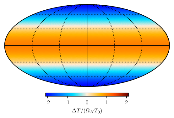
Figure 1: Fluctuations in the observed temperature, $\Delta T/T_{0}$, induced by background evolution in $S^{2}\times\mathbb{R}$ and $\mathbb{H}^{2}\times\mathbb{R}$, in units of the curvature parameter $\Omega_{K}$ and in the standard Mollweide projection.

CMB temperature anisotropies have been measured on large scales (most reliably by the WMAP [5] and Planck [25] teams). To be consistent with these observations the expansion-induced anisotropy must be sufficiently small. The CMB power spectrum is defined as

$$D_{\ell}\equiv\frac{\ell(\ell+1)}{2\pi}C_{\ell}\qquad\mbox{with}\qquad C_{\ell}=\frac{1}{2\ell+1}\sum_{m=-\ell}^{\ell}|a_{\ell m}|^{2}.$$ (4.33)

In this case, only $D_{2}$ is non-zero,

$$D_{2}\approx\frac{48}{25}F(\lambda_{r})^{2}\Omega_{K}^{2}T_{0}^{2}.$$ (4.34)

The observed $D_{2}$ reported in the most recent Planck data release [25] is

$$D_{2}^{\mathrm{obs}}=225.9\,\mathrm{\mu K^{2}}.$$ (4.35)

A limit is obtained on $\Omega_{K}$ by ensuring that the power in the induced quadrupole does not exceed that of the observed one,

$$|\Omega_{K}|\lesssim\frac{5}{4\sqrt{3}|F(\lambda_{r})|}\frac{\sqrt{D_{2}^{\mathrm{obs}}}}{T_{0}}\approx 3.8\times 10^{-6}$$ (4.36)

for $S^{2}\times\mathbb{R}$ and $\mathbb{H}^{2}\times\mathbb{R}$ spacetimes where we have chosen $T_{0}=2.726\,\mathrm{K}$ [26]. This is considerably more stringent than the $\Omega_{K}=0.001\pm 0.002$ bound reported by Planck [27] for the isotropic FLRW spaces.

5 $\widetilde{U(\mathbb{H}^{2})}$ and Nil

In the following sections, we will repeat the procedure outlined in Section 4 for the remaining three anisotropic Thurston spacetimes, starting with the spacetime of $\widetilde{U(\mathbb{H}^{2})}$. This section also contains the constraint on $\Omega_{K}$ in Nil since its metric is extremely similar to that of $\widetilde{U(\mathbb{H}^{2})}$ to the order at which we work.

5.1 $\widetilde{U(\mathbb{H}^{2})}$

As in the previous section, the metric for $\widetilde{U(\mathbb{H}^{2})}$ can be written in terms of the dimensionless parameter $\Omega_{K}$. Using Eq. 3.11 we have

$$-\kappa=-\frac{3}{k^{(0)}}H_{0}^{2}\Omega_{K}=\frac{12}{5}H_{0}^{2}\Omega_{K}.$$ (5.1)

Writing all coordinates in units of $H_{0}^{-1}$ we find

$$\mathrm{d}s^{2} =-\mathrm{d}t^{2}+a(t)^{2}\mathrm{d}x^{2}+{}$$ (5.2)

$$\quad\qquad{}+b(t)\left[a(t)\cosh\!\left(4\sqrt{\frac{3}{5}}\sqrt{\Omega_{K}}x\right)\mathrm{d}y^{2}+b(t)\mathrm{d}z^{2}+2a(t)\sinh\!\left(2\sqrt{\frac{3}{5}}\sqrt{\Omega_{K}}x\right)\mathrm{d}y\mathrm{d}z\right].$$

where we have used the identification $a_{1}(t)=a_{2}\equiv a(t)$ and $a_{3}(t)\equiv b(t)$. This identification ensures consistency with an isotropic stress energy to order $\sqrt{\Omega_{K}}$. Expanding the metric to this order and using (3.24) we see that the scale factors can be replaced with $A^{(0)}(t)$ leading to

$$\mathrm{d}s^{2}\approx-\mathrm{d}t^{2}+A^{(0)}(t)^{2}\left[\mathrm{d}x^{2}+\mathrm{d}y^{2}+\mathrm{d}z^{2}+4\sqrt{\frac{3}{5}}\sqrt{\Omega_{K}}x\mathrm{d}y\mathrm{d}z\right],$$ (5.3)

where now $\approx$ denotes equivalence to order $\sqrt{\Omega_{K}}$.

The equations for the null geodesics of this spacetime to order $\sqrt{\Omega_{K}}$ are

$$\frac{1}{A^{(0)}(t)^{2}}\frac{\mathrm{d}}{\mathrm{d}\lambda}\!\left[A^{(0)}(t)^{2}x^{\prime}(\lambda)\right]-2\sqrt{\frac{3}{5}}\sqrt{\Omega_{K}}y^{\prime}(\lambda)z^{\prime}(\lambda) \approx 0,$$

$$\frac{1}{A^{(0)}(t)^{2}}\frac{\mathrm{d}}{\mathrm{d}\lambda}\!\left[A^{(0)}(t)^{2}y^{\prime}(\lambda)\right]+2\sqrt{\frac{3}{5}}\sqrt{\Omega_{K}}z^{\prime}(\lambda)x^{\prime}(\lambda) \approx 0,$$ (5.4)

$$\frac{1}{A^{(0)}(t)^{2}}\frac{\mathrm{d}}{\mathrm{d}\lambda}\!\left[A^{(0)}(t)^{2}z^{\prime}(\lambda)\right]+2\sqrt{\frac{3}{5}}\sqrt{\Omega_{K}}x^{\prime}(\lambda)y^{\prime}(\lambda) \approx 0,$$

accompanied by a null condition (4.8)

$$t^{\prime}(\lambda)^{2}\approx A^{(0)}(t)^{2}\left[x^{\prime}(\lambda)^{2}+y^{\prime}(\lambda)^{2}+z^{\prime}(\lambda)^{2}+4\sqrt{\frac{3}{5}}\sqrt{\Omega_{K}}x(\lambda)y^{\prime}(\lambda)z^{\prime}(\lambda)\right].$$ (5.5)

The first order solutions in $\sqrt{\Omega_{K}}$ to (5.1–5.5) can be directly integrated from

$$x^{\prime}(\lambda) \approx\frac{1}{A^{(0)}(\lambda)^{2}}\!\left[c_{x}+2\sqrt{\frac{3}{5}}c_{y}c_{z}\sqrt{\Omega_{K}}S(\lambda)\right],$$

$$y^{\prime}(\lambda) \approx\frac{1}{A^{(0)}(\lambda)^{2}}\!\left[c_{y}-2\sqrt{\frac{3}{5}}c_{x}c_{z}\sqrt{\Omega_{K}}S(\lambda)\right],$$ (5.6)

$$z^{\prime}(\lambda) \approx\frac{1}{A^{(0)}(\lambda)^{2}}\!\left[c_{z}-2\sqrt{\frac{3}{5}}c_{x}c_{y}\sqrt{\Omega_{K}}S(\lambda)\right],$$

$$t^{\prime}(\lambda) \approx\frac{1}{A^{(0)}(\lambda)},$$

where $v(\lambda_{0})=1$ requires $c_{x}^{2}+c_{y}^{2}+c_{z}^{2}=1$, $A^{(0)}(\lambda)\equiv A^{(0)}(t(\lambda))$,

$$S(\lambda) \equiv H_{0}\int_{\lambda_{0}}^{\lambda}\frac{\mathrm{d}\lambda^{\prime}}{A^{(0)}(\lambda^{\prime})^{2}}=\int_{1}^{A^{(0)}(\lambda)}\frac{\mathrm{d}a^{\prime}}{a^{\prime 2}\sqrt{\Omega_{m}/a^{\prime 3}+\Omega_{\Lambda}}}$$ (5.7)

$$=\frac{1}{\sqrt{\Omega_{\Lambda}}}\left[\,\tensor[_{2}]{F}{{}_{1}}\!\left(\frac{1}{3},\frac{1}{2};\frac{4}{3};-\frac{\Omega_{m}}{\Omega_{\Lambda}}\right)-\frac{1}{A^{(0)}(\lambda)}\,\tensor[_{2}]{F}{{}_{1}}\!\left(\frac{1}{3},\frac{1}{2};\frac{4}{3};-\frac{\Omega_{m}}{A^{(0)}(\lambda)^{3}\Omega_{\Lambda}}\right)\right],$$

and we have chosen $A^{(0)}(\lambda_{0})=1$.

To compute the local photon flux (4.11) received by a present-day observer at the origin, we need to define local angular coordinates relating to solid angles in the sky. For this geometry, we again identify $\theta$ as the angle from the $z$-axis, permitting the use of (4.12) from the previous section. Writing the photon 3-velocity as $v^{i}(\lambda)=(x^{\prime}(\lambda),y^{\prime}(\lambda),z^{\prime}(\lambda))$ and expanding we find

$$\cos\theta\approx\frac{z^{\prime}(\lambda)\left[x^{\prime}(\lambda)^{2}+y^{\prime}(\lambda)^{2}+z^{\prime}(\lambda)^{2}\right]+2\sqrt{3/5}\sqrt{\Omega_{K}}x(\lambda)y^{\prime}(\lambda)\left[x^{\prime}(\lambda)^{2}+y^{\prime}(\lambda)^{2}\right]}{\left[x^{\prime}(\lambda)^{2}+y^{\prime}(\lambda)^{2}+z^{\prime}(\lambda)^{2}\right]^{3/2}}.$$ (5.8)

The velocities are given in (5.1) and the $x$ equation integrates to

$$x(\lambda)\approx c_{x}S(\lambda).$$ (5.9)

Plugging all of this in we find the very simple expression

$$\cos\theta\approx\frac{c_{z}}{\sqrt{c_{x}^{2}+c_{y}^{2}+c_{z}^{2}}},$$ (5.10)

which is a constant. In other words, photons propagate along lines of constant $\theta$ so that $\cos\theta_{0}\approx\cos\theta_{r}$.

Unlike the previous geometries, however, the polar angle $\varphi$ measured at recombination and today will differ since $\widetilde{U(\mathbb{H}^{2})}$ lacks rotational symmetry in its $xy$-plane. We choose to identify $\varphi$ as the angle from the $x$-axis within the $xy$-plane, meaning that

$$\tan\varphi=\frac{\tensor{g}{{}_{i}{}_{y}}v^{i}}{\tensor{g}{{}_{i}{}_{x}}v^{i}}\sqrt{\frac{\tensor{g}{{}_{x}{}_{x}}}{\tensor{g}{{}_{y}{}_{y}}}}.$$ (5.11)

Proceeding as above, expanding, and plugging in the velocities from (5.1) we find

$$\tan\varphi\approx\frac{y^{\prime}(\lambda)}{x^{\prime}(\lambda)}+2\sqrt{\frac{3}{5}}\sqrt{\Omega_{K}}x(\lambda)\frac{z^{\prime}(\lambda)}{x^{\prime}(\lambda)}\approx\frac{c_{y}}{c_{x}}-2\sqrt{\frac{3}{5}}\sqrt{\Omega_{K}}\left(\frac{c_{y}}{c_{x}}\right)^{2}c_{z}S(\lambda).$$ (5.12)

Evaluating (5.10) and (5.12) at $\lambda_{0}$ where $S(\lambda_{0})=0$ we find that these constants take the simple form of spherical coordinates:

$$(c_{x},c_{y},c_{z})=(\sin\theta_{0}\cos\varphi_{0},\sin\theta_{0}\sin\varphi_{0},\cos\theta_{0}).$$ (5.13)

Evaluating at recombination gives

$$\cos\theta_{r} \approx\cos\theta_{0},$$

$$\tan\varphi_{r} \approx\tan\varphi_{0}\left(1-2\sqrt{\frac{3}{5}}\sqrt{\Omega_{K}}S(\lambda_{r})\cos\theta_{0}\tan\varphi_{0}\right),$$ (5.14)

from which we determine the Jacobian factor

$$\frac{\mathrm{d}\Omega_{r}}{\mathrm{d}\Omega_{0}}\approx 1-2\sqrt{\frac{3}{5}}\sqrt{\Omega_{K}}S(\lambda_{r})\cos\theta_{0}\sin 2\varphi_{0}.$$ (5.15)

From (4.20), we know that the ratio of photon energies measured by observers today and at recombination is trivially

$$\frac{E(\lambda_{r})}{E(\lambda_{0})}\approx\frac{A^{(0)}(\lambda_{0})}{A^{(0)}(\lambda_{r})}$$ (5.16)

since spatial expansion is isotropic to order $\sqrt{\Omega_{K}}$. Similarly,

$$\frac{\mathrm{d}A_{r}\mathrm{d}t_{r}}{\mathrm{d}A_{0}\mathrm{d}t_{0}}\approx\left[\frac{A^{(0)}(\lambda_{r})}{A^{(0)}(\lambda_{0})}\right]^{3}.$$ (5.17)

Thus the photon flux measured by a present-day observer only receives nontrivial modifications from (5.15) and can be written as

$$\Phi(E_{0})\approx\frac{pE_{0}^{2}\left(1-2\sqrt{\frac{3}{5}}\sqrt{\Omega_{K}}S(\lambda_{r})\cos\theta_{0}\sin 2\varphi_{0}\right)}{\exp(E_{0}/T_{0})-1}$$ (5.18)

using (4.26).

This flux is qualitatively different than the flux (4.29) for $S^{2}\times\mathbb{R}$ and $\mathbb{H}^{2}\times\mathbb{R}$. Namely, an ${\cal O}(\sqrt{\Omega_{K})}$ correction appears as a direction-dependent but energy-independent factor, i.e., as a greybody factor to the entire expression, rather than as a direction-dependent factor on the temperature. The exponential term in the denominator is unmodified to this order. In this case, we cannot simply read off the observed CMB temperature from the exponent, and an effective temperature may instead be obtained from the total observed intensity $I$ integrated over all energies:

$$I=\int_{0}^{\infty}\mathrm{d}E_{0}\,E_{0}\Phi(E_{0}).$$ (5.19)

For a perfect blackbody of temperature $T$, this evaluates to

$$I=\frac{p\pi^{4}}{15}T^{4},$$ (5.20)

which is just the Stefan-Boltzmann law in our choice of units. With the anisotropic flux (5.18), the total observed intensity is

$$I\approx\frac{p\pi^{4}}{15}T_{0}^{4}\left(1-2\sqrt{\frac{3}{5}}\sqrt{\Omega_{K}}S(\lambda_{r})\cos\theta_{0}\sin 2\varphi_{0}\right).$$ (5.21)

Comparing (5.20) and (5.21), the effective CMB temperature can be identified as

$$T(\Omega_{0})\approx T_{0}\left(1-\frac{1}{2}\sqrt{\frac{3}{5}}\sqrt{\Omega_{K}}S(\lambda_{r})\cos\theta_{0}\sin 2\varphi_{0}\right)$$ (5.22)

to order $\sqrt{\Omega_{K}}$. For $\Omega_{m}=0.3$, $\Omega_{\Lambda}=0.7$, $A_{0}(\lambda_{r})=1/(1+z_{r})$, and $z_{r}=1090$ numerical evaluation of (5.7) gives $S(\lambda_{r})\approx-3.19$.

As in Section 4.3, we can decompose the observed temperature into spherical harmonics to constrain $\Omega_{K}$. This decomposition for (5.22) is more involved than in the previous section because the induced fluctuations cannot be represented with finitely many harmonics. We therefore save the details of this decomposition for Appendix B, and quote the results:

$$T(\Omega)\approx T_{0}\left\{1+\sqrt{\frac{3\pi}{5}}\sqrt{\Omega_{K}}S(\lambda_{r})\sum_{\begin{subarray}{c}\ell=3\\ \ell\text{ odd}\end{subarray}}^{\infty}\sqrt{2\ell+1}\sqrt{\frac{(\ell-2)!}{(\ell+2)!}}\mathrm{i}\left[Y_{\ell\,2}(\Omega)-Y_{\ell\,-2}(\Omega)\right]\right\}.$$ (5.23)

The corresponding normalized temperature fluctuations, $\Delta T(\Omega_{0})$, are shown in Fig. 2 in units of $\sqrt{\Omega_{K}}$.

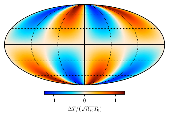
Figure 2: $\Delta T/T_{0}$ induced in $\widetilde{U(\mathbb{H}^{2})}$ in units of $\sqrt{\Omega_{K}}$.

The resulting octopole has the largest amplitude of the induced modes, and the constraint on $\Omega_{K}$ that follows from the induced octopole is

$$\Omega_{K}\lesssim\frac{50}{3S(\lambda_{r})^{2}}\frac{D_{3}^{\text{obs}}}{T_{0}^{2}}\approx 2\times 10^{-10}$$ (5.24)

where we have used $D_{3}^{\text{obs}}=936.9\,\mathrm{\mu K^{2}}$ again from Planck’s best-fit angular power spectrum [25]. Note that a much stronger constraint is reached here than for $S^{2}\times\mathbb{R}$ and $\mathbb{H}^{2}\times\mathbb{R}$ because modifications to the photon flux are introduced at $\mathcal{O}(\sqrt{\Omega_{K}})$ instead of $\mathcal{O}(\Omega_{K})$.

The astute reader will note that the induced temperature fluctuations extend to arbitrarily high $\ell$, with $D_{\ell}\propto\ell^{-1}$, whereas the conventional damping tail of CMB temperature falls as $\exp(-\ell^{2}/\ell_{D}^{2})$ (for some cosmological-parameter dependent value of $\ell_{D}$). This implies that, above some threshold $\ell$, the induced $D_{\ell}$ will exceed the usual predicted values, and ever-stricter limits on $\Omega_{K}$ will result form measurements of the CMB above that threshold. For the Plank best-fit FLRW cosmological parameters, that threshold is at $\ell>4000$, and thus somewhat above the highest $\ell$ that have been measured.

5.2 Nil

The constraint on curvature of the Nil spacetime largely mirrors that of $\widetilde{U(\mathbb{H}^{2})}$. Here

$$-\kappa=-\frac{3}{k^{(0)}}H_{0}^{2}\Omega_{K}=12H_{0}^{2}\Omega_{K},$$ (5.25)

a factor of 5 larger than in $\widetilde{U(\mathbb{H}^{2})}$, so expressing all coordinates in units of $H_{0}^{-1}$ the metric is

$$\mathrm{d}s^{2}=-\mathrm{d}t^{2}+a(t)^{2}\mathrm{d}x^{2}+b(t)\left[a(t)(1+12\Omega_{K}x^{2})\mathrm{d}y^{2}+b(t)\mathrm{d}z^{2}-4\sqrt{3}a(t)\sqrt{\Omega_{K}}x\mathrm{d}y\mathrm{d}z\right].$$ (5.26)

Though this differs from the metric Eq. 5.2 for $\widetilde{U(\mathbb{H}^{2})}$, expanding to order $\sqrt{\Omega_{K}}$

$$\mathrm{d}s^{2}\approx-\mathrm{d}t^{2}+A^{(0)}(t)^{2}\left[\mathrm{d}x^{2}+\mathrm{d}y^{2}+\mathrm{d}z^{2}-4\sqrt{3}\sqrt{\Omega_{K}}x\mathrm{d}y\mathrm{d}z\right].$$ (5.27)

This is the same as the ${\cal O}({\sqrt{\Omega_{K}}})$ metric Eq. 5.3 for $\widetilde{U(\mathbb{H}^{2})}$, with the off-diagonal term flipped in sign and multiplied by $\sqrt{5}$. It is unsurprising, then, that the modes induced in the observed CMB temperature strongly resembles those in $\widetilde{U(\mathbb{H}^{2})}$,

$$T(\theta_{0},\varphi_{0})\approx T_{0}\left[1-\sqrt{5}\sqrt{\Omega_{K}}S(\lambda_{r})\sum_{\begin{subarray}{c}\ell=3\\ \ell\text{ odd}\end{subarray}}^{\infty}\mathrm{i}\alpha_{\ell}(Y_{\ell\,2}-Y_{\ell\,-2})\right].$$ (5.28)

The $\Omega_{K}$ constraint in the Nil spacetime is

$$\Omega_{K}\lesssim\frac{10}{3S(\lambda_{r})^{2}}\frac{D_{3}^{\text{obs}}}{T_{0}^{2}}\approx 4\times 10^{-11},$$ (5.29)

which is stronger than the $\Omega_{K}$ constraint in $\widetilde{U(\mathbb{H}^{2})}$ by the expected factor of $5$, the ratio of the $k^{(0)}$’s between the two spacetimes.

6 Solv

The last anisotropic Thurston spacetime is Solv with metric given by

$$\mathrm{d}s^{2}=-\mathrm{d}t^{2}+a(t)^{2}\left[\mathrm{e}^{2z\sqrt{-\kappa}}\mathrm{d}x^{2}+\mathrm{e}^{-2z\sqrt{-\kappa}}\mathrm{d}y^{2}\right]+b(t)^{2}\mathrm{d}z^{2},$$ (6.1)

where we have identified $a_{1}(t)=a_{2}(t)\equiv a(t)$ and $a_{3}(t)=b(t)$. As in the other geometries, we rewrite $\kappa$ in terms of $\Omega_{K}$ and write the coordinates in units of $H_{0}^{-1}$ to express the metric as

$$\mathrm{d}s^{2}=-\mathrm{d}t^{2}+a(t)^{2}\left[\mathrm{e}^{2\sqrt{3}z\sqrt{\Omega_{K}}}\mathrm{d}x^{2}+\mathrm{e}^{-2\sqrt{3}z\sqrt{\Omega_{K}}}\mathrm{d}y^{2}\right]+b(t)^{2}\mathrm{d}z^{2},$$ (6.2)

As in $\widetilde{U(\mathbb{H}^{2})}$ and Nil, $\Omega_{K}$ appears with half-integer powers in the metric. It is natural to guess, then, that modifications to the CMB photon flux will appear at $\mathcal{O}(\sqrt{\Omega_{K}})$, but this is not the case. To $\mathcal{O}(\sqrt{\Omega_{K}})$, Solv experiences isotropic expansion, and no distortions to the local photon flux are induced. Therefore, to see effects in Solv it proves necessary to work to $\mathcal{O}(\Omega_{K})$. Also in contrast to $\widetilde{U(\mathbb{H}^{2})}$ and Nil general progress can be made without immediately expanding in powers of $\sqrt{\Omega_{K}}$. The geodesics of (6.2) are given by

$$\frac{1}{a(t)^{2}}\frac{\mathrm{d}}{\mathrm{d}\lambda}\!\left[a(t)^{2}x^{\prime}(\lambda)\right]+2\sqrt{3\Omega_{K}}x^{\prime}(\lambda)z^{\prime}(\lambda)=0,$$

$$\frac{1}{a(t)^{2}}\frac{\mathrm{d}}{\mathrm{d}\lambda}\!\left[a(t)^{2}y^{\prime}(\lambda)\right]-2\sqrt{3\Omega_{K}}y^{\prime}(\lambda)z^{\prime}(\lambda)=0,$$ (6.3)

$$\frac{1}{b(t)^{2}}\frac{\mathrm{d}}{\mathrm{d}\lambda}\!\left[b(t)^{2}z^{\prime}(\lambda)\right]-\sqrt{3\Omega_{K}}\left(\frac{a(t)}{b(t)}\right)^{2}\left[\mathrm{e}^{2\sqrt{3}z(\lambda)\sqrt{\Omega_{K}}}x^{\prime}(\lambda)^{2}-\mathrm{e}^{-2\sqrt{3}z(\lambda)\sqrt{\Omega_{K}}}y^{\prime}(\lambda)^{2}\right]=0,$$

along with a null condition (4.8)

$$t^{\prime}(\lambda)^{2}=a(t)^{2}\left[\mathrm{e}^{2\sqrt{3}z(\lambda)\sqrt{\Omega_{K}}}x^{\prime}(\lambda)^{2}+\mathrm{e}^{-2\sqrt{3}z(\lambda)\sqrt{\Omega_{K}}}y^{\prime}(\lambda)^{2}\right]+b(t)^{2}z^{\prime}(\lambda)^{2}.$$ (6.4)

The spatial equations are solved exactly to give velocities along null geodesics

$$x^{\prime}(\lambda) =c_{x}\frac{\mathrm{e}^{-2\sqrt{3}z(\lambda)\sqrt{\Omega_{K}}}}{a(\lambda)^{2}},$$

$$y^{\prime}(\lambda) =c_{y}\frac{\mathrm{e}^{2\sqrt{3}z(\lambda)\sqrt{\Omega_{K}}}}{a(\lambda)^{2}},$$ (6.5)

$$z^{\prime}(\lambda) =\frac{c_{z}}{b(\lambda)^{2}}+\sqrt{3\Omega_{K}}\frac{c_{x}x(\lambda)-c_{y}y(\lambda)}{b(\lambda)^{2}},$$

which can be substituted into (6.4) to find $t^{\prime}(\lambda)$.

In deriving the CMB photon flux today, we make the same definitions of angular coordinates ($\theta,\varphi$) as above, permitting the use of (4.12) and (5.11). Using these expression we find that $\theta_{r}$ and $\varphi_{r}$ depend on $\theta_{0}$ and $\varphi_{0}$ as

$$\cos\theta_{r} \approx\cos\theta_{0}+\sqrt{3\Omega_{K}}S(\lambda_{r})\sin^{2}\theta_{0}\cos 2\varphi_{0}-3\Omega_{K}\left[2F(\lambda_{r})+S(\lambda_{r})^{2}\right]\cos\theta_{0}\sin^{2}\theta_{0},$$ (6.6)

$$\tan\varphi_{r} \approx\tan\varphi_{0}\left[1+2\sqrt{3\Omega_{k}}S(\lambda_{r})\cos\theta_{0}+3\Omega_{K}S(\lambda_{r})^{2}\left(2\cos^{2}\theta_{0}+\sin^{2}\theta_{0}\cos 2\varphi_{0}\right)\right],$$

where $\approx$ denotes equivalence to $\mathcal{O}(\Omega_{K})$, $F(\lambda)$ is defined in (3.14), $S(\lambda)$ is defined in (5.7), and we have used the fact that

$$H_{0}\int_{\lambda_{0}}^{\lambda}\frac{S(\lambda^{\prime})\mathrm{d}\lambda^{\prime}}{{A^{(0)}(\lambda^{\prime})}^{2}}=\frac{1}{2}S(\lambda)^{2}.$$ (6.7)

The determinant of the Jacobian matrix gives

$$\frac{\mathrm{d}\Omega_{r}}{\mathrm{d}\Omega_{0}}\approx 1+3\Omega_{K}(1+3\cos 2\theta_{0})F(\lambda_{r}).$$ (6.8)

As noted above the leading order correction is $\mathcal{O}(\Omega_{K})$. The remaining geometric factor is

$$\frac{\mathrm{d}A_{r}\mathrm{d}t_{r}}{\mathrm{d}A_{0}\mathrm{d}t_{0}}=\frac{a(t_{r})^{2}b(t_{r})}{a(t_{0})^{2}b(t_{0})}\approx\left(\frac{A^{(0)}(\lambda_{r})}{A^{(0)}(\lambda_{0})}\right)^{3}\left[1+3\Omega_{K}\frac{A^{(1)}(\lambda_{r})}{A^{(0)}(\lambda_{r})}\right].$$ (6.9)

Similarly the energy factor that appears is

$$\frac{E_{r}^{2}\mathrm{d}E_{r}}{E_{0}^{2}\mathrm{d}E_{0}}\approx\left(\frac{A^{(0)}(\lambda_{0})}{A^{(0)}(\lambda_{r})}\right)^{3}\left\{1-3\Omega_{K}\left[(1+3\cos 2\theta_{0})F(\lambda_{r})+\frac{A^{(1)}(\lambda_{r})}{A^{(0)}(\lambda_{r})}\right]\right\}.$$ (6.10)

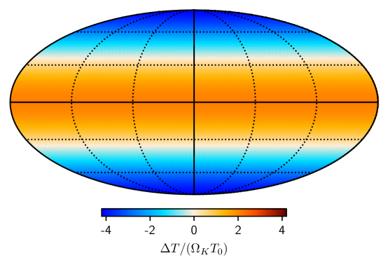
Figure 3: $\Delta T/T_{0}$ induced in Solv in units of $\Omega_{K}$.

Finally, combining the factors (6.8), (6.9), and (6.10), we find they all cancel in the same, perhaps surprising manner as in Section 4. This leads to the flux

$$\Phi(E_{0})\approx\frac{pE_{0}^{2}}{\exp(E_{r}/T_{0})-1},$$ (6.11)

where

$$T(\Omega_{0})\approx T_{0}\left[1+\Omega_{K}(1+3\cos 2\theta)F(\lambda_{r})\right].$$ (6.12)

From this we can write the temperature anisotropy induced in Solv as

$$\Delta T(\Omega_{0})\equiv T(\Omega_{0})-T_{0}\approx T_{0}\Omega_{K}(1+3\cos 2\theta)F(\lambda_{r}),$$ (6.13)

twice that found in Eq. 4.30 for $\mathbb{H}^{2}\times\mathbb{R}$. Decomposed into spherical harmonics we again see only a $Y_{20}(\Omega)$ contribution

$$\frac{\Delta T(\Omega)}{T_{0}}\approx 8\sqrt{\frac{\pi}{5}}\Omega_{K}F(\lambda_{r})Y_{20}(\Omega_{0}),$$ (6.14)

which is plotted in Fig. 3 in units of $\Omega_{K}$. For $z_{r}=1090$, $\Omega_{m}=0.3$, and $\Omega_{\Lambda}=0.7$ we have seen that $F(\lambda_{r})\approx-1.04$ and $S(\lambda_{r})\approx-3.19$. Finally, the bound on $\Omega_{K}$ is a factor of 2 stronger than that found for $\mathbb{H}^{2}\times\mathbb{R}$,

$$\Omega_{K}\lesssim\frac{5}{8\sqrt{3}|F(\lambda_{r})|}\frac{\sqrt{D_{2}^{\mathrm{obs}}}}{T_{0}}\approx 1.9\times 10^{-6}.$$ (6.15)

7 Conclusion

In this paper, we have, for the first time, derived powerful constraints on $\Omega_{K}$ in spacetimes with homogeneous anisotropic spatial geometries of all five corresponding Thurston types – $S^{2}\times\mathbb{R}$, $\mathbb{H}^{2}\times\mathbb{R}$, $\widetilde{U(\mathbb{H}^{2})}$, Nil, and Solv – when filled with standard homogeneous perfect-fluid dust and cosmological constant $\Lambda$. We have shown that, in $S^{2}\times\mathbb{R}$ and $\mathbb{H}^{2}\times\mathbb{R}$, CMB photons undergo direction-dependent redshift as they propagate from recombination through anisotropically expanding space. In $\widetilde{U(\mathbb{H}^{2})}$ and Nil, the underlying anisotropy of the three-geometry distorts the present-day local flux of CMB photons. An observer could interpret these effects as a blackbody with an anisotropic temperature, with an amplitude of anisotropy proportional to a power of $\sqrt{|\Omega_{K}|}$. We find that, in order for these temperature fluctuations to be no larger than the observed CMB anisotropies, $|\Omega_{K}|\lesssim 10^{-5}$ in $S^{2}\times\mathbb{R}$ and $\mathbb{H}^{2}\times\mathbb{R}$, $\Omega_{K}\lesssim 10^{-6}$ in Solv, and $\Omega_{K}\lesssim 10^{-10}$ in $\widetilde{U(\mathbb{H}^{2})}$ and Nil.

We have not commented on the impact of primordial perturbations on the observed CMB temperature. Though it is theoretically possible for this anisotropy to be exactly canceled out by temperature fluctuations existing at the time of last scattering, it is highly unlikely that we live just at the moment when such cancellation occurs.

We emphasize that these constraints are valid for a Universe filled with perfect fluid dust and cosmological constant, but do not necessarily hold for less conventional stress-energy contents. For instance, it has been shown that the CMB temperature maintains its isotropy in certain shear-free models sourced by a finely-tuned anisotropic fluid [28]. We note however that the angular diameter and luminosity distances are still direction-dependent in the shear-free renditions of anisotropic Thurston spacetimes [18], so it still may be possible to constrain anisotropy less stringently using other cosmological observables (e.g., see [29]).

Our powerful constraints come from comparison of observed CMB temperature fluctuations with the direction-dependent photon flux that results from the evolution of an isotropic homogeneous blackbody distribution at the time of recombination into an anisotropic photon distribution today. These constraints are therefore independent of the physics responsible for the usual primordial fluctuations.

Appendix A $\tensor{\Delta}{{}^{\mu}_{\nu}}$ in $\widetilde{U(\mathbb{H}^{2})}$ and Nil

Here we list out the entries of $\tensor{\Delta}{{}^{\mu}_{\nu}}$ in $\widetilde{U(\mathbb{H}^{2})}$ and Nil. For $\mu,\nu\in\{0,1\}$

$$\tensor{\Delta}{{}^{0}_{0}} =~{}-\tensor{\Delta}{{}^{1}_{1}} = -x^{2}\frac{3\Omega_{K}}{4k^{(0)}}\left[\frac{\dot{a}}{a}-\frac{\dot{b}}{b}\right]^{2}+\mathcal{O}(\Omega_{K}^{2})$$ (A.1)

$$\tensor{\Delta}{{}^{0}_{1}} =-a^{2}\tensor{\Delta}{{}^{1}_{0}} = -x\frac{3\Omega_{K}}{2k^{(0)}}\left[\frac{\dot{a}}{a}-\frac{\dot{b}}{b}\right]+\mathcal{O}(\Omega_{K}^{2}),$$ (A.2)

where we have set $a_{1}=a_{2}=a$ and $a_{3}=b$.

The remaining nontrivial elements of $\tensor{\Delta}{{}^{\mu}_{\nu}}$ are

$$\tensor{\Delta}{{}^{2}_{2}} =~{}~{} -x^{2}\frac{3\Omega_{K}}{4k^{(0)}}\left[\left(\frac{\dot{a}}{a}\right)^{2}-\left(\frac{\dot{b}}{b}\right)^{2}+\frac{2\ddot{a}}{a}-\frac{2\ddot{b}}{b}\right] +\mathcal{O}(\Omega_{K}^{2})$$ (A.3)

$$\tensor{\Delta}{{}^{2}_{3}} =~{}~{} \zeta x\sqrt{-\frac{3\Omega_{K}}{4k^{(0)}}}\left(\frac{b}{a}\right)\left[-\frac{\dot{a}\dot{b}}{ab}+\left(\frac{\dot{b}}{b}\right)^{2}-\frac{\ddot{a}}{a}+\frac{\ddot{b}}{b}\right] +\mathcal{O}(\Omega_{K}^{3/2})$$ (A.4)

$$\tensor{\Delta}{{}^{3}_{2}} =~{}~{} \zeta x\sqrt{-\frac{3\Omega_{K}}{4k^{(0)}}}\left(\frac{a}{b}\right)\left[2\left(\frac{\dot{a}}{a}\right)^{2}-\frac{\dot{3a}\dot{b}}{ab}+\left(\frac{\dot{b}}{b}\right)^{2}+\frac{\ddot{a}}{a}-\frac{\ddot{b}}{b}\right] +\mathcal{O}(\Omega_{K}^{3/2})$$ (A.5)

$$\tensor{\Delta}{{}^{3}_{3}} =~{}~{} x^{2}\frac{3\Omega_{K}}{4k^{(0)}}\left[3\left(\frac{\dot{a}}{a}\right)^{2}-\frac{4\dot{a}\dot{b}}{ab}+\left(\frac{\dot{b}}{b}\right)^{2}+\frac{2\ddot{a}}{a}-\frac{2\ddot{b}}{b}\right] +\mathcal{O}(\Omega_{K}^{2}),$$ (A.6)

where $\zeta=+1$ in Nil and $\zeta=-1$ in $\widetilde{U(\mathbb{H}^{2})}$.

From (3.12), we know $a$ and $b$ differ by an order $\Omega_{K}$ correction, meaning (A.1) and (A.2) are high enough order in $\Omega_{K}$ to be neglected. We may verify the same is true for the other nontrivial elements by using (3.12) to rewrite (A.3)–(A.6) as

$$\tensor{\Delta}{{}^{2}_{2}} =~{} -\tensor{\Delta}{{}^{3}_{3}} =~{} -x^{2}\frac{3\Omega_{K}^{2}}{2k^{0}}(K^{(1)}-K^{(3)})\left(\frac{3\dot{A}\dot{F}}{A}+\ddot{F}\right)+\mathcal{O}(\Omega_{K}^{2})$$ (A.7)

$$\tensor{\Delta}{{}^{2}_{3}} =~{} -\tensor{\Delta}{{}^{3}_{2}} =~{} -\zeta x\sqrt{\frac{-3\Omega_{K}^{3}}{4k^{0}}}(K^{(1)}-K^{(3)})\left(\frac{3\dot{A}\dot{F}}{A}+\ddot{F}\right)+\mathcal{O}(\Omega_{K}^{3/2}),$$ (A.8)

where $F=F[A(t)]$ is given by (3.14).

Appendix B Temperature fluctuation amplitudes in $\widetilde{U(\mathbb{H}^{2})}$ and Nil

Here we derive the spherical harmonic representation of the temperature (5.23) for $\widetilde{U(\mathbb{H}^{2})}$. This derivation can easily be extended to that for Nil given their similarities at $\mathcal{O}(\sqrt{\Omega_{K}})$. We begin with (5.22) written as

$$T(\Omega)\approx T_{0}\left(1-\frac{1}{2}\sqrt{\frac{3}{5}}\sqrt{\Omega_{K}}S(\lambda_{r})\cos\theta\sin 2\varphi\right),$$ (B.1)

where we have dropped subscripts from the angular components for brevity. From the $\sin 2\varphi$ factor we immediately see that only harmonic modes with $m=\pm 2$ will contribute, and they will have equal amplitude and opposite sign. Since $T(\Omega)$ is a real function we know that $a_{\ell 2}=a_{\ell-2}^{*}$ and thus $a_{\ell 2}$ is imaginary. Thus we only need to compute $m=+2$. To begin,

$$a_{\ell 2}\approx-\frac{1}{2}\sqrt{\frac{3}{5}}\sqrt{\Omega_{K}}S(\lambda_{r})\alpha_{\ell},$$ (B.2)

with

$$\alpha_{\ell}\equiv\int\cos\theta\sin 2\varphi\,Y_{\ell 2}^{*}(\Omega)\,\mathrm{d}\Omega.$$ (B.3)

Using the standard functional form

$$Y_{\ell 2}(\Omega)=\sqrt{\frac{2\ell+1}{4\pi}}\sqrt{\frac{(\ell-2)!}{(\ell+2)!}}P_{\ell}^{2}(\cos\theta)\mathrm{e}^{\mathrm{i}2\varphi},$$ (B.4)

and recalling that $P_{\ell}^{m}(-x)=(-1)^{\ell-m}P_{\ell}^{m}(x)$, we see that $\alpha_{\ell}=0$ for even $\ell$. Meanwhile, we will show below that

$$\int_{-1}^{1}xP_{\ell}^{2}(x)\,\mathrm{d}x=4\,,\qquad\ell\mbox{ odd}\,.$$ (B.5)

The required integral over $\varphi$ is

$$\int_{0}^{2\pi}\sin 2\varphi\,\mathrm{e}^{-2\mathrm{i}\varphi}\,\mathrm{d}\varphi=-\mathrm{i}\pi.$$ (B.6)

Thus

$$\alpha_{\ell}=\begin{cases}-2\mathrm{i}\sqrt{(2\ell+1)\pi}\sqrt{\frac{(\ell-2)!}{(\ell+2)!}}&\mbox{$\ell$ odd,}\\ 0&\mbox{$\ell$ even.}\end{cases}$$ (B.7)

Thus we find

$$a_{\ell 2}\approx\begin{cases}\mathrm{i}\sqrt{\frac{3(2\ell+1)\pi}{5}}\sqrt{\frac{(\ell-2)!}{(\ell+2)!}}S(\lambda_{r})\sqrt{\Omega_{K}}&\mbox{$\ell$ odd,}\\ 0&\mbox{$\ell$ even.}\end{cases}$$ (B.8)

so that

$$\frac{\Delta T(\Omega)}{\sqrt{\Omega_{K}}T_{0}}\approx\sqrt{\frac{3\pi}{5}}S(\lambda_{r})\sum_{\begin{subarray}{c}\ell=3\\ \ell\text{ odd}\end{subarray}}^{\infty}\sqrt{2\ell+1}\sqrt{\frac{(\ell-2)!}{(\ell+2)!}}\mathrm{i}\left[Y_{\ell 2}(\Omega)-Y_{\ell-2}(\Omega)\right],$$ (B.9)

as claimed in (5.23).

The integral in (B.5) can be evaluated as follows. From the recursion relation

$$xP_{\ell}^{2}(x)=\frac{1}{2\ell+1}\left[(\ell+2)P_{\ell-1}^{2}(x)+(\ell-1)P_{\ell+1}^{2}(x)\right]$$ (B.10)

the required integral is

$$\int_{-1}^{1}xP_{\ell}^{2}(x)\,\mathrm{d}x =\frac{1}{2\ell+1}\int_{-1}^{1}\left[(\ell+2)P_{\ell-1}^{2}(x)+(\ell-1)P_{\ell+1}^{2}(x)\right]\mathrm{d}x,$$

$$\equiv\frac{1}{2\ell+1}\left[(\ell+2)J_{\ell-1}+(\ell-1)J_{\ell+1}\right],$$ (B.11)

where we have defined for all $n\geq 2$

$$J_{n}\equiv\int_{-1}^{1}P_{n}^{2}(x)\,\mathrm{d}x.$$ (B.12)

This integral can be evaluated by first noting that from the definition of the associated Legendre functions in terms of the Legendre polynomials and Legendre’s equation we have

$$P_{n}^{2}(x)=(1-x^{2})\frac{\mathrm{d}^{2}P_{n}(x)}{\mathrm{d}x^{2}}=2x\frac{\mathrm{d}P_{n}(x)}{\mathrm{d}x}-n(n+1)P_{n}(x).$$ (B.13)

Employing the recursion relation

$$x\frac{\mathrm{d}P_{n}(x)}{\mathrm{d}x}=\frac{\mathrm{d}P_{n-1}(x)}{\mathrm{d}x}+nP_{n}(x)$$ (B.14)

we thus can write

$$P_{n}^{2}(x)=2\frac{\mathrm{d}P_{n-1}(x)}{\mathrm{d}x}-n(n-1)P_{n}(x).$$ (B.15)

We are left to evaluate

$$J_{n}=\int_{-1}^{1}\left[2\frac{\mathrm{d}P_{n-1}(x)}{\mathrm{d}x}-n(n-1)P_{n}(x)\right]\mathrm{d}x.$$ (B.16)

Orthogonality of the Legendre polynomials shows that the second term in the integrand integrates to zero (for $n\geq 2$). The first term in the integrand is a total derivative. Since $P_{n}(-1)=(-1)^{n}$ and $P_{n}(1)=1$ we arrive at

$$J_{n}=2P_{n-1}(x)\Bigr{|}_{-1}^{1}=2\left[1-(-1)^{n-1}\right]=\begin{cases}0,&n\mbox{ odd}\\ 4,&n\mbox{ even}\end{cases}$$ (B.17)

Finally, plugging this into (B) we arrive at the result quoted in (B.5).

References

- [1] A.A. Penzias and R.W. Wilson, A Measurement of Excess Antenna Temperature at 4080 Mc/s., Astrophys. J. 142 (1965) 419.
- [2] E. Abdalla et al., Cosmology intertwined: A review of the particle physics, astrophysics, and cosmology associated with the cosmological tensions and anomalies, JHEAp 34 (2022) 49 [arXiv:2203.06142].
- [3] Planck collaboration, Planck 2018 results. VII. Isotropy and Statistics of the CMB, Astron. Astrophys. 641 (2020) A7 [arXiv:1906.02552].
- [4] D.J. Schwarz, G.D. Starkman, D. Huterer and C.J. Copi, Is the low- microwave background cosmic?, Phys. Rev. Lett. 93 (2004) 221301 [astro-ph/0403353].
- [5] C.L. Bennett et al., First-Year Wilkinson Microwave Anisotropy Probe (WMAP) Observations: Preliminary Maps and Basic Results, Astrophys. J. Suppl. Ser. 148 (2003) 1 [astro-ph/0302207].
- [6] D.J. Schwarz, C.J. Copi, D. Huterer and G.D. Starkman, CMB Anomalies after Planck, Class. Quant. Grav. 33 (2016) 184001 [arXiv:1510.07929].
- [7] J. Jones, C.J. Copi, G.D. Starkman and Y. Akrami, The Universe is not statistically isotropic, arXiv:2310.12859.
- [8] G.F.R. Ellis, The Bianchi models: Then and now, Gen. Relativ. Gravit. 38 (2006) 1003.
- [9] L. Bianchi, On the three-dimensional spaces which admit a continuous group of motions, Soc. Ital. Sci. Mem. di Mat. 11 (1898) 267.
- [10] A. Pontzen, Rogues’ gallery: The full freedom of the Bianchi CMB anomalies, Phys. Rev. D 79 (2009) 103518 [arXiv:0901.2122].
- [11] R. Sung and P. Coles, Polarized Spots in Anisotropic Open Universes, Class. Quant. Grav. 26 (2009) 172001 [arXiv:0905.2307].
- [12] E. Martinez-Gonzalez and J.L. Sanz, and the isotropy of the universe, Astron. Astrophys. 300 (1995) 346.
- [13] D. Saadeh, S.M. Feeney, A. Pontzen, H.V. Peiris and J.D. McEwen, How Isotropic is the Universe?, Phys. Rev. Lett. 117 (2016) 131302 [arXiv:1605.07178].
- [14] T. Rothman and R. Matzner, Nucleosynthesis in anisotropic cosmologies revisited, Phys. Rev. D 30 (1984) 1649.
- [15] W.P. Thurston, Three dimensional manifolds, Kleinian groups and hyperbolic geometry, Bull. Amer. Math. Soc. 6 (1982) 357.
- [16] H.V. Fagundes, Relativistic Cosmologies with Closed, Locally Homogeneous Spatial Sections, Phys. Rev. Lett. 54 (1985) 1200.
- [17] P.W. Graham, R. Harnik and S. Rajendran, Observing the Dimensionality of Our Parent Vacuum, Phys. Rev. D 82 (2010) 063524 [arXiv:1003.0236].
- [18] Y. Awwad and T. Prokopec, Large-scale geometry of the Universe, JCAP 01 (2024) 010 [arXiv:2211.16893].
- [19] G. Perelman, The entropy formula for the ricci flow and its geometric applications, math.DG/0211159.
- [20] G. Perelman, Ricci flow with surgery on three-manifolds, math.DG/0303109.
- [21] COMPACT collaboration, Promise of Future Searches for Cosmic Topology, Phys. Rev. Lett. 132 (2024) 171501 [arXiv:2210.11426].
- [22] R. Kantowski and R.K. Sachs, Some Spatially Homogeneous Anisotropic Relativistic Cosmological Models, J. Math. Phys. 7 (1966) 443.
- [23] C.B. Collins, Shear-free fluids in general relativity., Can. J. Phys. 64 (1986) 191.
- [24] J.P. Mimoso and P. Crawford, Shear-free anisotropic cosmological models, Class. Quant. Grav. 10 (1993) 315.
- [25] Planck collaboration, Planck 2018 results. V. CMB power spectra and likelihoods, Astron. Astrophys. 641 (2020) A5 [arXiv:1907.12875].
- [26] J.C. Mather et al., Measurement of the Cosmic Microwave Background spectrum by the COBE FIRAS instrument, Astrophys. J. 420 (1994) 439.
- [27] Planck collaboration, Planck 2018 results. VI. Cosmological parameters, Astron. Astrophys. 641 (2020) A6 [arXiv:1807.06209].
- [28] T.S. Koivisto, D.F. Mota, M. Quartin and T.G. Zlosnik, Possibility of anisotropic curvature in cosmology, Phys. Rev. D 83 (2011) 023509 [arXiv:1006.3321].
- [29] T.S. Pereira, G.A.M. Marugán and S. Carneiro, Cosmological Signatures of Anisotropic Spatial Curvature, JCAP 07 (2015) 029 [arXiv:1505.00794].