Black hole singularity resolution from unitarity
Abstract
We study the quantum dynamics of an interior planar AdS (anti–de Sitter) black hole, requiring unitarity in the natural time coordinate conjugate to the cosmological “constant of motion” appearing in unimodular gravity. Both the classical singularity and the horizon are replaced by a non-singular highly quantum region; semiclassical notions of spacetime evolution are only valid in an intermediate region. For the singularity, our results should be applicable to general black holes: unitarity in unimodular time always implies singularity resolution.
Introduction. — The fate of classical singularities is one of the most important questions for any theory of quantum gravity; indeed, the incompleteness of classical relativity formalised in the Penrose–Hawking singularity theorems [1] is often cited as a main motivation for why gravity must be quantum. The most important singularities of direct relevance to our Universe are at the Big Bang and at the centre of black holes. In a first approximation, these situations can be represented through idealised, spatially homogeneous geometries whose high degree of symmetry allows for a quantum description at least at an effective level. One can then ask in such simple models what happens to the classical singularity.
In the context of homogeneous cosmology, the question of whether singularities are resolved through quantum effects (in what is usually called quantum cosmology) does not have a clear answer, since it depends both on the criteria for singularity resolution and on the precise definition of the model including the choice of quantum state [2]. Nevertheless, one can make general statements if the quantum theory is required to be unitary with respect to a given choice of time [3]: one would expect singularities to be resolved if they are only a finite “time” away for that specific notion of time, since singular evolution seems incompatible with the requirement of a global time translation operator. Inevitably, such a general result means that the property of singularity resolution depends on the choice of clock [4], and signifies a general clash between general covariance and the quantum notion of unitarity [5], in itself a somewhat controversial topic in quantum gravity.
Here we note that the results of Ref. [4] extend straightforwardly to the study of black hole singularities, in particular for the planar AdS black holes studied in Ref. [6] and related previous work in the context of AdS/CFT [7]. The interior metric studied in these works is of Kasner type, with a single anisotropy variable, and dynamically equivalent to a flat homogeneous, isotropic cosmology with a massless scalar field. The cosmological constant is taken to be negative and fixed, but reinterpreting it as a constant of motion as suggested by unimodular gravity [8] turns it into another global degree of freedom. The black hole interior is then classically identical to the cosmology studied in [4], and its canonical quantisation can be studied along the same lines. If the Schrödinger-like time coordinate conjugate to the cosmological constant is used to define evolution, and one requires the theory to be unitary, all singularities are resolved [9].
The notion of “singularity” in this context does not only apply to curvature singularities; a singularity is any point at which the classical evolution terminates, and where non-classical behaviour is necessarily required for a unitary quantum theory. These can be coordinate singularities [5]. In our black hole model, at the horizon the spatial volume goes to zero and the classical solution cannot continue. Quantum unitarity with respect to the preferred clock (here unimodular time) would then require the horizon to be similarly replaced by a highly quantum region in which classical evolution is not valid. This specific conclusion is sensitive to the particular choice of foliation which becomes singular at the horizon. However, the conclusion regarding black hole singularities is more generally valid since the singularity is only a finite time away for many possible observers. The Belinski–Khalatnikov–Lifshitz (BKL) conjecture states that approach to a generic singularity is described by Kasner-like dynamics, like the example studied here; this suggests that for many possible clock choices, the classical singularity would need to be replaced by well-defined quantum evolution leading to the emergence of a white hole. Our results demonstrate that black hole singularities either lead to a failure of quantum unitarity (in unimodular time), or to a new scenario for a quantum transition of a black hole to a white hole.
Quantum theory of black hole interior. — The classical action for general relativity with cosmological constant , including the Gibbons–Hawking–York boundary term, is
| (1) |
where is the spacetime metric, the Ricci scalar, the boundary metric and the extrinsic curvature; where is Newton’s constant.
The interior planar black hole (Kasner) metric studied in Ref. [6] and previous papers [7] is given by
| (2) |
where , and are functions of only. Thought of as a radial coordinate outside the horizon, in the interior is timelike and hence this metric is spatially homogeneous. It corresponds to a locally rotationally symmetric Bianchi I model with metric written in the Misner parametrisation (see, e.g., Ref. [10]). One important feature of this parametrisation is that the anisotropy variables (here a single one, ) behave as free massless scalar fields in a flat isotropic geometry, as we will see explicitly.
Substituting the metric ansatz (2) into (1) reduces the action to
| (3) |
where ′ denotes derivative with respect to . We have implicitly assumed that the overall numerical factor arising from performing the integration over , and has been set to one by a choice of coordinates.
Legendre transform leads to a Hamiltonian
| (4) |
where we have made the unit choice to obtain a simpler form. The resulting Hamiltonian constraint [6]
| (5) |
is exactly the one studied in Ref. [4], where it was interpreted as describing a flat homogeneous, isotropic cosmology with a free massless scalar field and a perfect fluid (playing the rôle of dark energy). In this interpretation, is no longer a parameter but a (conserved) momentum conjugate to a time variable . This assumption can be justified by promoting in (3) to a dynamical variable and adding a term to the action. The resulting action is then the reduction of the Henneaux–Teitelboim action for unimodular gravity [11]
| (6) |
with suitable boundary terms to a spatially homogeneous geometry. See also Ref. [12] for a more general perspective on “deconstantisation” applied to other quantities; we only need the statement that is an integration constant, familiar from unimodular gravity.
The classical solutions in the time are found to be
| (7) | ||||
| (8) |
where and are integration constants. The metric 2 has singularities () for and . The Kretschmann scalar
| (9) |
diverges for (black hole singularity, ) but is finite for (black hole horizon, ).
The constraint (5) can be written as , making the dynamical problem equivalent to relativistic particle motion in a configuration space (minisuperspace) parametrised by and and with a flat metric
| (10) |
This minisuperspace is equivalent to the Rindler wedge, a portion of full (1+1) dimensional Minkowski spacetime with boundary at . This viewpoint suggests a natural operator ordering in canonical quantisation [4, 6, 13, 14], leading to the Wheeler–DeWitt equation
| (11) |
where is the Laplace–Beltrami operator for . Eq. (11) is covariant with respect to variable transformations of and and, because is flat, with respect to lapse redefinitions which act as conformal transformations on [15].
The general solution to Eq. (11) can be straightforwardly given as
| (12) |
where and are so far arbitrary and is a Bessel function of the first kind. Eq. (12) gives the general solution as a function of , a dynamical variable in our setup; for it is less ambiguous to pass from to the modified Bessel functions and [4]. The appearance of Bessel function solutions for the black hole interior is familiar from other contexts [16]. Fourier transform converts the wavefunction given as a function of into a time-dependent wavefunction dependent on , the conjugate to .
Asking whether the resulting quantum theory is unitary with respect to evolution in unimodular time 111To see why is unimodular time, note the global factor in the Hamiltonian . For to be given just by the constraint , we must choose so that is constant. is equivalent to asking whether is self-adjoint in a suitable inner product. The most natural choice of inner product is induced by ,
| (13) |
It is easy to see is then not self-adjoint, as expected for a space with boundaries which can be reached by classical solutions in a finite amount of time. Here this corresponds to both the black hole horizon and the singularity being only a finite (unimodular) time away. Self-adjoint extensions can be defined by restricting wavefunctions to a subspace satisfying the boundary condition [4, 9]
| (14) |
thus obtaining a unitary quantum theory. Such a boundary condition can be seen as reflection from the singularity, similar to what is proposed in Ref. [14].
We are interested in solutions, which are the analogue of bound states. Normalised solutions to the Wheeler–DeWitt equation 11 and the boundary condition 14 can be expressed as
| (15) |
where and
| (16) |
is a discrete set of allowed negative values. Here the free function parametrises different self-adjoint extensions of ; in a sense, each choice of defines a different theory. Qualitative features explored in the following are not expected to be sensitive to this choice, as shown in a similar model in loop quantum cosmology [17]. For simplicity, we choose below.
Eq. 15 represents the quantum states of a planar AdS black hole interior as superpositions of different values of momentum and cosmological constant . Crucially, because of the reflecting boundary condition the allowed bound states are modified Bessel functions of the second kind, behaving near as
| (17) |
i.e., as superpositions of positive and negative modes with equal magnitude. Since changing the sign of is equivalent to time reversal, swapping the roles of horizon and singularity, or switching between classical black-hole and white-hole solutions (see Eq. (9) and below; this corresponds to the parameter in the classical solution), none of these bound states can correspond to a single semiclassical trajectory that ends in a singularity. The necessary superpositions of black-hole and white-hole solutions then lead to singularity resolution in this theory.
Singularity resolution. — To see this explicitly, we numerically study the evolution of a semiclassical (Gaussian) state
| (18) |
with free parameters , , , and and a normalisation factor . For a semiclassical interpretation we need , and . The latter condition then also guarantees that the allowed discrete values are reasonably close together.
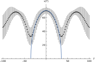
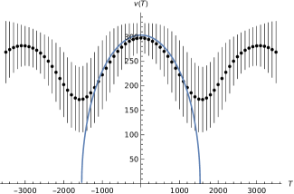
Our main observable is the volume . Expectation values and moments of in our state take the form
| (19) |
the integral in Eq. (19) can be done analytically, leaving the sums and the integral for numerical evaluation. In practice, due to the Gaussians inside the integral the contributions from and are very small and we can replace the infinite integral and sums over and by finite sums by introducing cutoffs.
The expectation value can be compared with classical solutions given in Eq. (7) where and are replaced by the average of and in our chosen states; due to the discrete spacing of possible values these averages are not exactly equal (but close) to and .
In Fig. 1 we show the quantum expectation value and fluctuations for such a state (with two different sets of parameters). We can see that, as expected from the general discussion, for small the expectation value stays close to its corresponding classical solution (7), but it departs strongly near the horizon or singularity where the interference between an ingoing (black hole) and outgoing (white hole) solution becomes important. There is a finite minimal value for and in this sense, both the black hole singularity and the horizon are replaced by quantum “bounces”. When the expectation value closely follows the classical curve, the variance is small, indicating that the state is indeed semiclassical, but at the bounces the variance grows, indicating strong quantum fluctuations where the state is reflected. As required by unitarity, all expectation values and higher moments are globally defined, not just for the finite interval in which the classical solution is valid. Taken at face value the resulting quantum solution describes cycles of local expansion and contraction, corresponding to a sequence of black hole/white hole interiors passing from horizon to singularity and back. We see that over longer timescales the variances grow, suggesting a spreading in the state and eventual breakdown of the semiclassical picture. While all the specific features displayed here depend on the chosen parameters in the state, the qualitative behaviour showing disappearance of the classical horizon and singularity seems universal, resulting from the reflecting boundary condition (14).
Discussion. — It has long been stated that a quantum theory of black hole dynamics that is required to be unitary must deviate strongly from semiclassical expectations. Usually this is discussed in the context of unitarity of black hole formation and evaporation, leading to the famous issue of information loss [18]. Preserving unitarity together with a few other “reasonable” assumptions can lead to disasters such as a firewall at the horizon [19], or more generally the conclusion that there is no simple semiclassical resolution of the paradox. What we are discussing here is different; we studied a simple quantum model of the black hole interior, in which the gravitational degrees of freedom (in the truncation to a Kasner metric) are quantised according to the Wheeler–DeWitt equation. In this setting too, there is a clash between unitarity and consistency with semiclassical physics: unitarity means globally well-defined time evolution, which is incompatible with singularities or even the appearance of a coordinate singularity at the horizon. It is of course a tricky issue to define unitarity in a fundamentally timeless setting such as canonical quantum gravity. The key ingredient in our discussion was to use unimodular gravity and its preferred choice of time coordinate, which can be implemented through auxiliary fields as in Ref. [11]. With respect to this clock, both the horizon and the singularity are only a finite time away, as they would be for an infalling observer. Unitarity forces us to replace both the horizon and the singularity with highly quantum bounce regions. Unitarity with respect to a different notion of clock would generally lead to different conclusions, showing a clash between unitarity and general covariance [5]. Our general conclusions should be valid for any standard of time such that the singularity or horizon are only a finite time away. It would be interesting to construct other analytically accessible examples.
The work of Ref. [6] studied a number of possible clocks in the same interior black hole spacetime. For instance, the anisotropy parameter is classically monotonic, and hence a good standard of time. With respect to this clock and other clocks such as (or ) and , no deviation from semiclassical physics was found in Ref. [6]. These observations are fully consistent with the results of Ref. [4] for the and clocks, and with the general conjecture of Ref. [3], where different clocks were classed as “slow” and “fast”. Unitarity with respect to a fast clock, which runs to at a singularity, does not require any deviation from semiclassical physics. In the black hole model studied here, , and are all fast. Similar behaviour is also found, for example, for a massless scalar field clock in homogeneous Wheeler–DeWitt cosmology [20]. However, such clocks do not describe the experience of local observers; classical singularities are troublesome exactly because one can reach them in finite time. When such a slow clock is studied, on approach to the singularity one must either give up unitarity or find generic resolution of all singularities, and possibly horizons.
The metric form (2) corresponds to a simple model of a black hole with planar symmetry, but only a slight extension – adding a second possible anisotropy variable in the Misner parametrisation – turns it into the general Kasner form describing, according to the BKL conjecture, successive periods during the generic approach to a spacelike singularity, even for more complicated or realistic black holes (as discussed in the related work of Ref. [14]). Since this second anisotropy variable again acts as a massless scalar field in an isotropic Universe, the results illustrated here would be expected to hold more generically for singularities. For horizons, the general picture is less clear since the model studied here sees the horizon as a coordinate singularity, and the black hole metric at a horizon would in general be more complicated. Already in the case of the usual (A)dS-Schwarzschild black hole, the positive curvature of constant time slices would contribute at the horizon and potentially change the conclusions. In general, it is at least in principle always possible to construct a model with a notion of time that stays regular at the horizon, so that collapse from an asymptotically flat (or asymptotically AdS or de Sitter) region could be described as a unitary process. While all of these alternative constructions will change the interpretation of what happens at the horizon, in the theory we have defined unitary quantum dynamics will always necessarily replace the (universal) singularity by non-singular evolution into a white hole: either unitarity fails, or there is no black hole singularity.
Acknowledgments. — The work of SG is funded by the Royal Society through the University Research Fellowship Renewal URFR221005. LMP is supported by the Leverhulme Trust.
References
- [1] S. W. Hawking and G. F. R. Ellis, The large scale structure of space-time (Cambridge University Press, 1973).
- [2] V. Husain and O. Winkler, “Singularity resolution in quantum gravity,” Phys. Rev. D 69 (2004) 084016, gr-qc/0312094; A. Ashtekar, “Singularity resolution in loop quantum cosmology: A brief overview,” J. Phys. Conf. Ser. 189 (2009) 012003, arXiv:0812.4703; C. Kiefer, “On the avoidance of classical singularities in quantum cosmology,” J. Phys. Conf. Ser. 222 (2010) 012049.
- [3] M. J. Gotay and J. Demaret, “Quantum cosmological singularities,” Phys. Rev. D 28 (1983), 2402–2413.
- [4] S. Gielen and L. Menéndez-Pidal, “Singularity resolution depends on the clock,” Class. Quant. Grav. 37 (2020) 205018, arXiv:2005.05357; “Unitarity, clock dependence and quantum recollapse in quantum cosmology,” Class. Quant. Grav. 39 (2022) 075011, arXiv:2109.02660; L. Menéndez-Pidal, The problem of time in quantum cosmology (PhD Thesis, University of Nottingham, 2022), arXiv:2211.09173.
- [5] S. Gielen and L. Menéndez-Pidal, “Unitarity and quantum resolution of gravitational singularities,” Int. J. Mod. Phys. D 31 (2022) 2241005, arXiv:2205.15387.
- [6] S. A. Hartnoll, “Wheeler–DeWitt states of the AdS–Schwarzschild interior,” JHEP 01 (2023) 066, arXiv:2208.04348.
- [7] J. P. S. Lemos, “Two-dimensional black holes and planar general relativity,” Class. Quant. Grav. 12 (1995) 1081–1086, gr-qc/9407024; E. Witten, “Anti-de Sitter space, thermal phase transition, and confinement in gauge theories,” Adv. Theor. Math. Phys. 2 (1998) 505–532, hep-th/9803131; A. Frenkel, S. A. Hartnoll, J. Kruthoff and Z. D. Shi, “Holographic flows from CFT to the Kasner universe,” JHEP 08 (2020) 003, arXiv:2004.01192; N. Bilic and J. C. Fabris, “Thermodynamics of AdS planar black holes and holography,” JHEP 11 (2022) 013, arXiv:2208.00711.
- [8] J. L. Anderson and D. Finkelstein, “Cosmological constant and fundamental length,” Am. J. Phys. 39 (1971) 901–904; J. J. van der Bij, H. van Dam and Y. J. Ng, “The Exchange of Massless Spin Two Particles,” Physica 116A (1982) 307–320; W. G. Unruh, “Unimodular theory of canonical quantum gravity,” Phys. Rev. D 40 (1989) 1048–1052; W. Buchmüller and N. Dragon, “Einstein Gravity From Restricted Coordinate Invariance,” Phys. Lett. B 207 (1988) 292-294; “Gauge Fixing and the Cosmological Constant,” Phys. Lett. B 223 (1989) 313–317.
- [9] S. Gryb and K. P. Y. Thébault, “Superpositions of the cosmological constant allow for singularity resolution and unitary evolution in quantum cosmology,” Phys. Lett. B 784 (2018) 324–329, arXiv:1801.05782; “Bouncing Unitary Cosmology I: Mini-Superspace General Solution,” Class. Quant. Grav. 36 (2019) 035009, arXiv:1801.05789; “Bouncing Unitary Cosmology II: Mini-Superspace Phenomenology,” Class. Quant. Grav. 36 (2019) 035010, arXiv:1801.05826.
- [10] M. Bojowald, Canonical Gravity and Applications: Cosmology, Black Holes, and Quantum Gravity (Cambridge University Press, 2010).
- [11] M. Henneaux and C. Teitelboim, “The cosmological constant and general covariance,” Phys. Lett. B 222 (1989) 195–199.
- [12] J. Magueijo, “Cosmological time and the constants of nature,” Phys. Lett. B 820 (2021) 136487, arXiv:2104.11529.
- [13] S. W. Hawking and D. N. Page, “Operator ordering and the flatness of the universe,” Nucl. Phys. B 264 (1986), 185–196.
- [14] M. J. Perry, “No Future in Black Holes,” arXiv:2106.03715.
- [15] J. J. Halliwell, “Derivation of the Wheeler–DeWitt equation from a path integral for minisuperspace models,” Phys. Rev. D 38 (1988) 2468–2481.
- [16] M. Bouhmadi-López, S. Brahma, C. Y. Chen, P. Chen and D. h. Yeom, “Annihilation-to-nothing: a quantum gravitational boundary condition for the Schwarzschild black hole,” JCAP 11 (2020) 002, arXiv:1911.02129.
- [17] T. Pawłowski and A. Ashtekar, “Positive cosmological constant in loop quantum cosmology,” Phys. Rev. D 85 (2012) 064001, arXiv:1112.0360.
- [18] S. W. Hawking, “Breakdown of predictability in gravitational collapse,” Phys. Rev. D 14 (1976) 2460–2473.
- [19] A. Almheiri, D. Marolf, J. Polchinski and J. Sully, “Black holes: complementarity or firewalls?,” JHEP 02 (2013) 062, arXiv:1207.3123.
- [20] A. Ashtekar and P. Singh, “Loop quantum cosmology: a status report,” Class. Quant. Grav. 28 (2011) 213001, arXiv:1108.0893.