Galaxy assembly bias in the stellar-to-halo mass relation for red central galaxies from SDSS

Abstract

We report evidence of galaxy assembly bias — the correlation between galaxy properties and biased secondary halo properties at fixed halo mass (M_H) — in the stellar-to-halo mass relation (SHMR) for red central galaxies from the Sloan Digital Sky Survey. In the M${}_{\mathrm{H}}=10^{11.5}-10^{13.5}~{}h^{-1}$ M_⊙ range, central galaxy stellar mass (M_∗) is correlated with the number density of galaxies within $10~{}h^{-1}$ Mpc ($\delta_{10}$), a common proxy for halo formation time. This galaxy assembly bias signal is also present when M_H, M_∗, and $\delta_{10}$ are substituted with group luminosity, galaxy luminosity, and metrics of the large-scale density field. To associate differences in $\delta_{10}$ with variations in halo formation time, we fitted a model that accounts for (1) errors in the M_H measured by the Tinker (2021, 2022) group catalog and (2) the level of correlation between halo formation time and M_∗ at fixed M_H. Fitting of this model yields that (1) errors in M_H are $\sim 0.15$ dex and (2) halo formation time and M_∗ are strongly correlated (Spearman’s rank correlation coefficient $\sim 0.85$). At fixed M_H, variations of $\sim 0.4$ dex in M_∗ are associated with $\sim 1-3$ Gyr variations in halo formation time and in galaxy formation time (from stellar population fitting; Oyarzún et al. 2022). These results are indicative that halo properties other than M_H can impact central galaxy assembly.

1 Introduction

In the current cosmological picture, the growth of dark-matter halos and the formation of galaxies are closely connected (e.g. White & Rees 1978; Blumenthal et al. 1984; Mo & White 1996; Wechsler & Tinker 2018; Vogelsberger et al. 2020). As halo mass (M_H) increases, so does the gravitational pull of the halo, facilitating the accretion of gas, fueling star-formation, and promoting the build-up of stellar mass (M_∗). The resulting correlation between M_H and M_∗ is known as the stellar-to-halo mass relation of central galaxies (SHMR; e.g. Moster et al. 2013).

While M_H emerges as the primary halo property driving galaxy growth, simulations of galaxy formation indicate that halo properties other than M_H also play a role. One of these properties is thought to be halo formation time (e.g. Gao et al. 2005; Tojeiro et al. 2017). Variations in halo assembly history lead to variations in halo gravitational potential with time, ultimately impacting the M_∗ assembly history of the galaxies that they host (e.g. Wechsler et al. 2002, 2006; Gao et al. 2005; Li et al. 2008). Similarly, halos of different concentrations feature different radial dark-matter density profiles, affecting the assembly histories of halos and galaxies alike, according to simulations (Ludlow et al. 2014; Matthee et al. 2017; Xu & Zheng 2020). These correlations between galaxy properties and biased secondary halo properties at fixed M_H that are apparent in theoretical work are known as galaxy assembly bias (e.g. Croton et al. 2007; Mao et al. 2017; Zehavi et al. 2018; Hadzhiyska et al. 2021, 2023; Montero-Dorta & Rodriguez 2024).

The major role played by dark-matter halos in simulations of galaxy formation has encouraged observational studies to search for signatures of galaxy-halo co-evolution. For instance, Obuljen et al. (2020) found the power spectrum of galaxies in the Baryon Oscillation Spectroscopic Survey of SDSS-III (BOSS; Dawson et al. 2013) to vary with galaxy central stellar velocity dispersion. These variations — of the order of $5\sigma$ — appear at spatial scales that extend beyond the virial radii of dark-matter halos, indicating that galaxy properties correspond with the distribution of halos in the large scale structure. In a separate study, Wang et al. (2022) found that the spatial distribution of galaxies in the Sloan Digital Sky Survey (SDSS; Alam et al. 2015) was best reproduced with halo occupation models (e.g. Tinker et al. 2008) that account for galaxy assembly bias in halo concentration. The same conclusion was reached by Yuan et al. (2021) in BOSS and by Pearl et al. (2023) in the Dark Energy Spectroscopic Instrument (DESI) One-Percent Survey (DESI Collaboration et al. 2016). Taken together, these recent studies suggest that galaxy assembly bias is apparent in the spatial distribution of galaxies in the nearby Universe.

Despite the mounting observational evidence in support of galaxy assembly bias, the connection between secondary halo properties and galaxy properties (e.g. stellar mass or star-formation rate; Kauffmann 2015) remains unconstrained due to challenges affecting observational studies of the galaxy-halo connection. For instance, signatures of one-halo conformity, i.e., the similarity in the observable properties of galaxies within a halo (Weinmann et al. 2006), can be interpreted as evidence of galaxy assembly bias. However, because these signatures can also be explained by the co-evolution between central and satellite galaxies (e.g. Pasquali et al. 2010; Peng et al. 2012; Wetzel et al. 2013; Cortese et al. 2019; Gallazzi et al. 2020; Oyarzún et al. 2023) and by systematic errors (e.g. Calderon et al. 2018), using one-halo conformity as a probe for galaxy assembly bias can be difficult. While other work (e.g. Kauffmann et al. 2013) have attempted to mitigate these degeneracies by searching for signatures of galaxy assembly bias in two-halo conformity instead (the similarity between the physical properties of galaxies in neighboring halos; e.g. Lacerna et al. 2022), biases in the isolation criterion emerge as a major concern (Sin et al. 2017; Tinker et al. 2018).

Instead of studying the impact of galaxy assembly bias on galaxy formation through galactic conformity, other work have turned to the clustering of galaxies. Studies have reported variations in the clustering signal with galaxy environment (Lehmann et al. 2017; Zentner et al. 2019) and/or galaxy color (Montero-Dorta et al. 2017). However, the reliability of these results has been questioned in light of systematic errors affecting the photometric group catalogs used for estimating halo masses (Campbell et al. 2015; Lin et al. 2016).

With systematic errors hampering observational studies of the galaxy-halo connection, recent efforts have focused on mitigating some of these shortcomings. For instance, the group catalog by Tinker (2021, 2022) is calibrated with observations of color-dependent galaxy clustering and estimates of the total satellite luminosity, which allows for a more accurate reproduction of the central galaxy quenched fraction. In addition, Tinker (2021) used deep photometry from the DESI Legacy Imaging Survey (DLIS; Dey et al. 2019), allowing for precise accounting of galaxy M_∗ and total group luminosity (L_group).

For instance, in Oyarzún et al. (2022) we exploited the Tinker (2021) catalog to estimate the M_H for over 2000 central galaxies in the SDSS-IV MaNGA survey (Mapping Nearby Galaxies at Apache Point Observatory; Bundy et al. 2015) and identified variations in the stellar populations of central galaxies at fixed M_H. Specifically, central galaxies with high M_∗ for their M_H feature old and Mg-enhanced stellar components. These results, along with equivalent trends recovered in spatially unresolved spectroscopy from the SDSS (Scholz-Díaz et al. 2022, 2023, 2024), are an indication that variations in the assembly histories of central galaxies cannot be fully ascribed to variations in M_H, thus hinting that halo properties other than M_H may play a role in central galaxy formation.

In this paper, we test whether these variations in the observable properties of central galaxies at fixed M_H can be attributed to galaxy assembly bias. To this end, we quantify how halo formation time varies within the SHMR for $\sim$ 150,000 red central galaxies from the SDSS main Galaxy Survey (MGS; York et al. 2000; Gunn et al. 2006; Alam et al. 2015) by utilizing the number density of galaxies within a radius of $R=10~{}h^{-1}$ Mpc (Alpaslan & Tinker 2020). The association between halo formation time and the number density of galaxies is motivated by how higher density regions of the large scale structure form at earlier cosmic epochs (e.g. Hahn et al. 2007; Lee et al. 2017).

This manuscript is organized as follows. We present our dataset in Section 2, methodology in Section 3, and results in Section 4. We discuss the implications of our work in Section 5 and summarize in Section 6. This paper makes use of the spectroscopic M_∗ measured by Chen et al. (2012) and the M_H estimated by Tinker (2021). The M_∗ adopt a Kroupa (2001) IMF and $h=0.7$. All magnitudes are reported in the AB system (Oke & Gunn 1983).

2 Dataset

2.1 Galaxy sample

To study the SHMR for central galaxies in the nearby Universe, we turned to the largest sample of nearby galaxies publicly available, the SDSS main Galaxy Survey sample (MGS; York et al. 2000; Gunn et al. 2006; Alam et al. 2015). In particular, we used the dr72bright34 subsample of the MGS, which was defined in the construction of the NYU Value-Added Galaxy Catalog (NYU-VAC; Blanton et al. 2005). Spectroscopic and photometric data outputs are available as part of the eighth data release (DR8) of the SDSS (Brinchmann et al. 2004). To limit biases in the survey selection function, we restricted our sample of central galaxies to the redshift range $0.04<z<0.16$, yielding 434,811 galaxies. To identify central galaxies in the MGS, we turned to the halo-based galaxy group catalog for SDSS by Tinker (2021). We selected all galaxies with satellite probabilities $P_{sat}<0.1$, resulting in 299,409 central galaxies. Further details on the group finder algorithm that we used to identify central galaxies are presented in Section 2.2.

Because group catalogs can imprint systematic errors into the M_H distributions of red and blue galaxies, separating the two populations is recommended (Lin et al. 2016). To separate red and blue galaxies in the MGS, we followed the Gaussian-mixture model employed by Tinker (2021). This model operates in the space composed of the 4000 Å break index (D${}_{n}4000$) and galaxy luminosity (L${}_{\mbox{\scriptsize gal}}$). The outputs of the model were fitted, yielding a threshold of

$$\begin{split}&\mbox{D${}_{n}^{\mbox{\scriptsize crit}}4000$}(\mbox{L${}_{\mbox{\scriptsize gal}}$})=\\ 1.42+\frac{0.35}{2}&\left[1+\texttt{erf}\left(\frac{\log{\mbox{L${}_{\mbox{\scriptsize gal}}$}}-9.9}{0.8}\right)\right]\end{split}$$ (1)

to separate the two populations. Here, erf(x) is the error function. We refer the reader to Tinker (2021) for more details on how the threshold D${}_{n}^{\mbox{\scriptsize crit}}4000(\mbox{L${}_{\mbox{\scriptsize gal}}$})$ was fitted to SDSS data.

This characterization of D${}_{n}^{\mbox{\scriptsize crit}}4000(\mbox{L${}_{\mbox{\scriptsize gal}}$})$ was used to identify and remove all blue central galaxies. The resulting sample contains 142,292 red central galaxies, which constitutes the working sample of this study. A sample of red central galaxies has two benefits over a sample of blue central galaxies. First, the majority of centrals are red at the high halo mass end (e.g. Yang et al. 2007), which is where the halo masses are the most reliable (e.g. Tinker 2022). Second, our prior characterization of the assembly histories of centrals within the SHMR focused on a passive sample (Oyarzún et al. 2022), which better corresponds with a red sample.

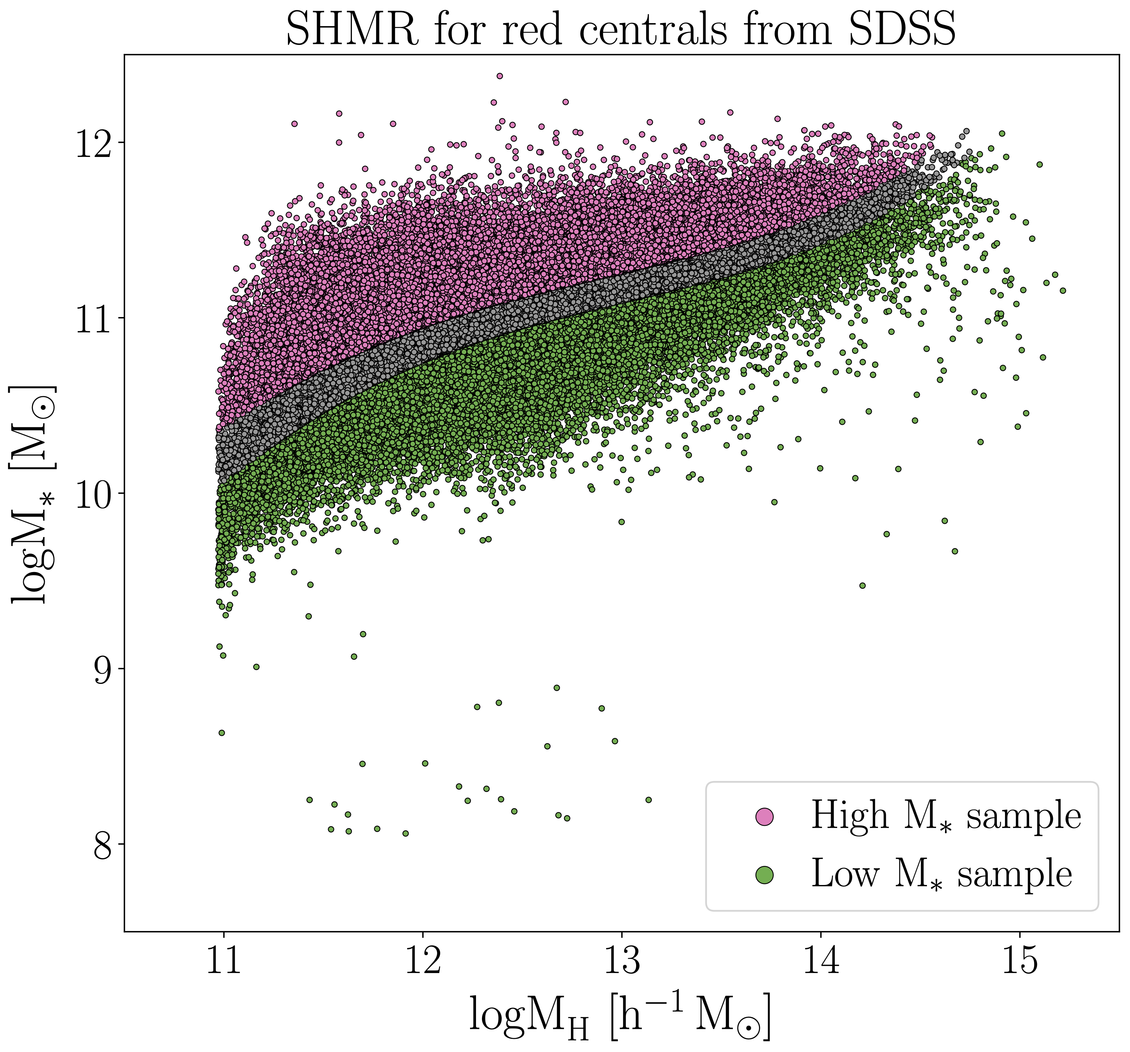
Figure 1: Stellar-to-halo mass relation for red central galaxies from SDSS. The M_∗ were measured in spectra from the SDSS by Chen et al. (2012) and the M_H were estimated with the group-finding algorithm by Tinker (2022) on deep photometry from the DLIS (Tinker 2021). We used the 33rd and 66th percentiles in M_∗-to-M_H ratio to divide centrals into high M_∗ (magenta) and low M_∗ (green) subsamples.

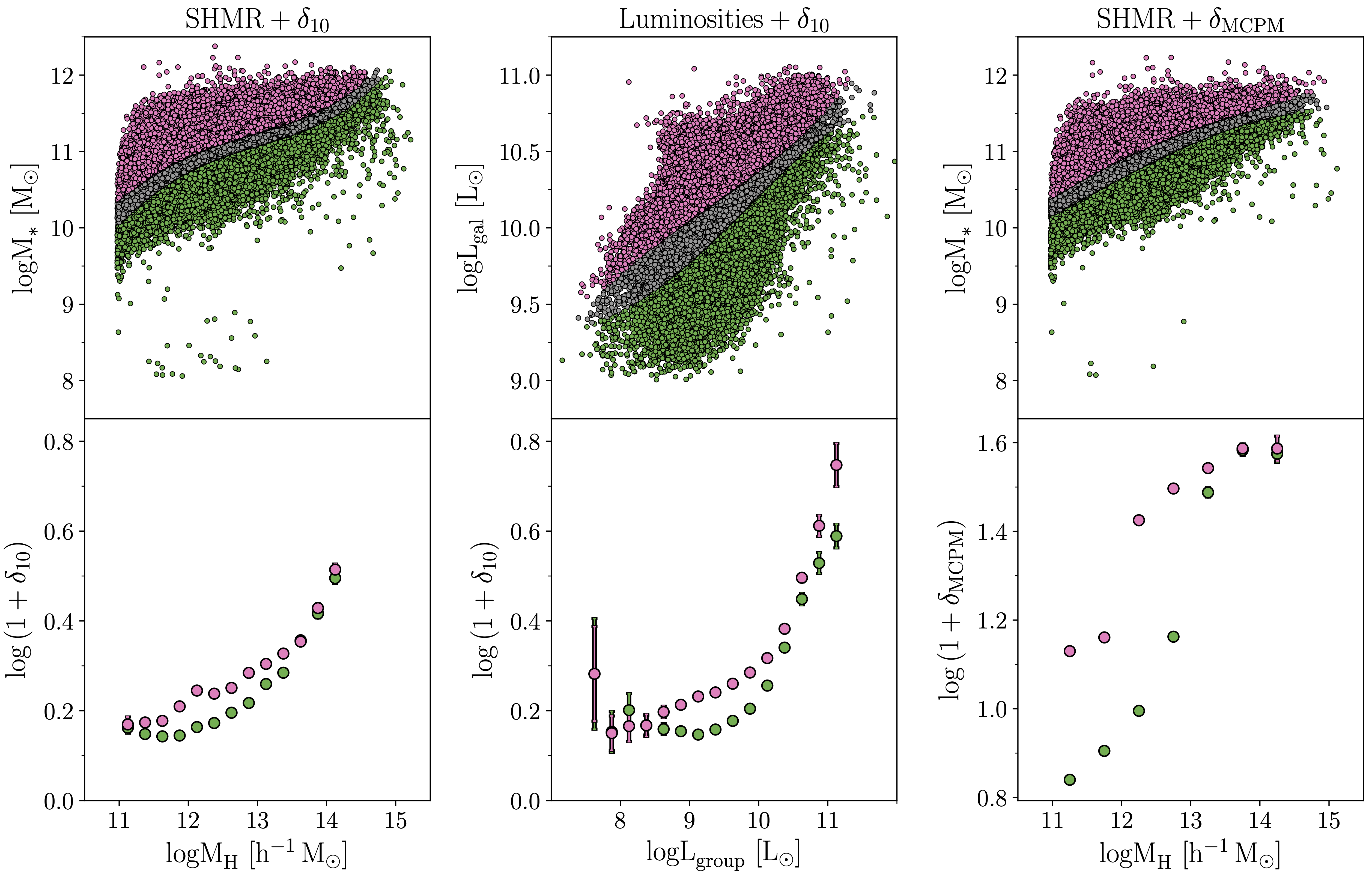
Figure 2: Left: The top panel shows the stellar-to-halo mass relation for red central galaxies from SDSS (same as Figure 1). The bottom panel shows the number density of galaxies within a radius $R=10~{}h^{-1}$ Mpc as a function of halo mass. High M_∗ centrals have higher galaxy number densities than low M_∗ centrals. Middle: Same as the left panel but with galaxy r-band luminosity instead of stellar mass and total group r-band luminosity instead of halo mass. Right: Same as the left panel, albeit with galaxy number density substituted with a metric of the density field measured with the MCPCM Slime Mold reconstruction of the Cosmic Web (Burchett et al. 2020). Apparent in all three panels is how galaxy stellar mass (or luminosity) varies with proxies for the density of the large scale structure at fixed halo mass (or at fixed group luminosity).

2.2 Halo masses

For the identification of central galaxies and to obtain estimates of their M_H, we utilized the halo-based galaxy group finder by Tinker (2022). In this algorithm, the probability of a galaxy being a central depends on both galaxy type and luminosity, enabling accurate reproduction of the central galaxy quenched fraction. After central galaxies and their corresponding groups are determined, halo masses are assigned through abundance matching with the Bolshoi-Planck simulation (Klypin et al. 2016). At this point, color-dependent galaxy clustering and total satellite luminosity are utilized as observational constraints until the best fitting model is found.

For our analysis, we worked with the publicly available implementation of the Tinker (2022) algorithm on SDSS (Tinker 2021). To construct the catalog, Tinker (2021) used deep photometry from the DESI Legacy Imaging Survey (DLIS; Dey et al. 2019), allowing for more accurate accounting of galaxy M_∗ and group L_∗ than in other group catalogs. The M_H for our sample of red central galaxies is shown in Figure 1.

2.3 Stellar masses

The M_∗ were retrieved from the SDSS DR8 outputs. They were measured by Chen et al. (2012) as part of a PCA-based approach to constrain the star-formation histories and stellar populations for galaxies from SDSS DR7 and BOSS (Aihara et al. 2011). The small scatter at fixed halo mass shown by these stellar masses ($\sim 0.18$ dex) make them ideal for this work (Tinker et al. 2017). To measure their M_∗, Chen et al. (2012) modeled the optical wavelength range between 3700 Å and 5500 Å of every spectrum with a linear combination of seven eigenspectra. The model space was constructed by generating a spectral library spanning a wide variety of star-formation histories. In this work, we retrieved the M_∗ that used the Maraston & Strömbäck (2011) stellar population synthesis models and Kroupa (2001) IMF for the construction of the library.

To determine whether some of the scatter in the red SHMR is driven by secondary halo properties (e.g. Zentner et al. 2014; Xu & Zheng 2020), we defined two subsamples of red central galaxies at fixed M_H: high-M_∗ and low-M_∗ centrals. These samples were computed as the 33rd and 66th percentiles in M_∗-to-M_H ratio, in similar fashion to Oyarzún et al. (2022). In equation form,

$$\begin{split}\mbox{High-M${}_{*}$ sample: }&\frac{\mbox{M${}_{*}$}}{\mbox{M${}_{\mathrm{H}}$}}(\mbox{M${}_{\mathrm{H}}$})>\left[\frac{\mbox{M${}_{*}$}}{\mbox{M${}_{\mathrm{H}}$}}(\mbox{M${}_{\mathrm{H}}$})\right]_{.66}\\ \mbox{Low-M${}_{*}$ sample: }&\frac{\mbox{M${}_{*}$}}{\mbox{M${}_{\mathrm{H}}$}}(\mbox{M${}_{\mathrm{H}}$})<\left[\frac{\mbox{M${}_{*}$}}{\mbox{M${}_{\mathrm{H}}$}}(\mbox{M${}_{\mathrm{H}}$})\right]_{.33}.\end{split}$$ (2)

The two subsamples are plotted in Figure 1. High-M_∗ centrals are plotted in magenta and low-M_∗ centrals are plotted in green.

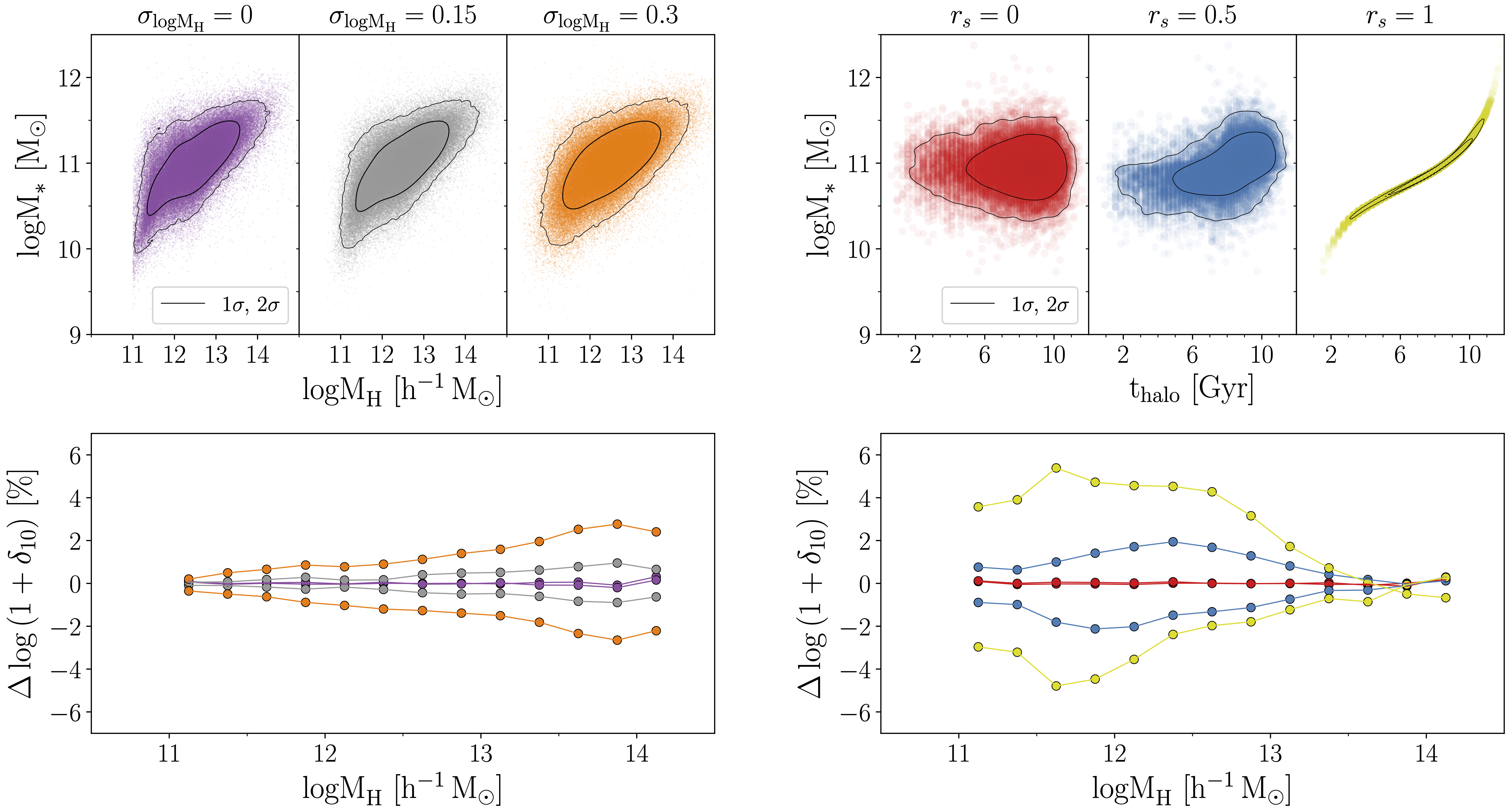
Figure 3: Model for interpreting variations in the number density of galaxies with M_∗ at fixed M_H. The free parameters of the model are the random error in the halo mass estimates from the group catalog ($\sigma_{\log{\mathrm{M}_{\mathrm{H}}}}$) and the Spearman’s rank correlation coefficient ($r_{s}$) between $\mathrm{t}_{\mathrm{halo}}$ and M_∗ at fixed M_H (i.e., the galaxy assembly bias signal). Left: The SHMR for red central galaxies from SDSS for different values of $\sigma_{\log{\mathrm{M}_{\mathrm{H}}}}$ (top). Differences in $\Delta\log(1+\delta_{10})$ between high-M_∗ and low-M_∗ centrals for the different values of $\sigma_{\log{\mathrm{M}_{\mathrm{H}}}}$ (bottom). Right: The correlation between $\mathrm{t}_{\mathrm{halo}}$ and M_∗ for different values of $r_{s}$ in the M${}_{\mathrm{H}}=10^{12.25}-10^{12.5}~{}h^{-1}$ M_⊙ bin (top). Variations in $\Delta\log(1+\delta_{10})$ between high-M_∗ and low-M_∗ centrals for the different values of $r_{s}$ (bottom). We note how $\sigma_{\log{\mathrm{M}_{\mathrm{H}}}}$ and $r_{s}$ are only partially degenerate, allowing us to simultaneously quantify their impact on $\Delta\log(1+\delta_{10})$.

3 Methodology

3.1 Galaxy number densities and halo formation times

In $\Lambda$CDM, higher density regions of the large scale structure collapse at earlier cosmic epochs (Lemson & Kauffmann 1999). We can take advantage of this property of $\Lambda$CDM to use the normalized number density of galaxies within a large radius $R$ as our observational proxy for halo formation time.

In principle, any radius larger than the sizes of halos (i.e., $R\gtrsim 1~{}h^{-1}$ Mpc) should suffice. However, scales $R\lesssim 5~{}h^{-1}$ Mpc are not ideal because splashback subhalos can magnify the halo assembly bias signal (e.g. Sunayama et al. 2016). Moreover, our ability to decouple the effects of M_H and halo formation time on central galaxy M_∗ improves as $R$ increases. For these reasons, $R\gtrsim 10~{}h^{-1}$ Mpc are preferred (Mansfield & Kravtsov 2020). In this work, we opted for $R=10~{}h^{-1}$ Mpc to keep the computation time manageable.

The number density of galaxies within $R=10~{}h^{-1}$ Mpc (hereafter $\delta_{10}$) was computed for every central as

$$\delta_{10}=\frac{\rho_{z}}{\langle\rho_{z}\rangle}-1,$$ (3)

where $\rho_{z}$ is the number density of galaxies around a top-hat sphere of radius $R=10~{}h^{-1}$ Mpc and $\langle\rho_{z}\rangle$ is the average $\rho_{z}$ at the redshift of the central. These two quantities were estimated in simulations that randomized the spatial distribution of galaxies, and they account for incompleteness and for edge effects. Further details on how $\delta_{10}$ was computed can be found in Alpaslan & Tinker (2020). The average value of $\delta_{10}$ as a function of M_H for our red central galaxies is shown in Figure 2.

To connect galaxy number density and halo formation time, we turned to the MultiDark Planck 2 Simulation (MDPL2; Prada et al. 2012). We first measured M_H, $\delta_{10}$, and $\mathrm{t}_{\mathrm{halo}}$ for every host halo in the simulation, where $\mathrm{t}_{\mathrm{halo}}$ is the lookback time at which the host halo assembled half of its total mass at $z=0$ (e.g. Tojeiro et al. 2017). Although all halo formation times reported in this manuscript were obtained according to the aforementioned definition, the main conclusions of this paper also stand if we instead use $\mathrm{t}_{\mathrm{halo}}^{11.5}$, which corresponds to the lookback time at which a critical halo mass of M${}_{\mathrm{H}}=10^{11.5}~{}h^{-1}$ M_⊙ was reached (more in Section 4).

For the measurement of the number density of galaxies in MDPL2, only subhalos with $V_{\mathrm{peak}}>100$ km s^-1 were counted, where $V_{\mathrm{peak}}$ is the maximum peak circular rotation velocity across all redshifts. This choice can be interpreted as counting only subhalos with M${}_{\mathrm{H}}\gtrsim 10^{11}~{}h^{-1}$ M_⊙ (Kravtsov et al. 2004; Zehavi et al. 2019). Then, we ensured that the dynamic range of $\delta_{10}$ in the data and in the simulation were comparable. To this end, we implemented an abundance matching approach, i.e., the halos were rank ordered in $\delta_{10}$ at fixed M_H and their $\delta_{10}$ values were matched.

3.2 Galaxy assembly bias model

Here, we describe the analytical model we used to associate differences in $\delta_{10}$ at fixed M_H with variations in halo formation time. Our model has two parameters: the error in the M_H reported by the group catalog and the strength of the correlation between halo formation time and stellar mass at fixed M_H.

Imprecise halo mass estimates can broaden the observed scatter of the SHMR, potentially biasing our high-M_∗ and low-M_∗ subsamples (see Figure 1). To account for this effect, we added random perturbations to the measured halo masses prior to the sample assignment step (Section 2.3). These random perturbations were drawn from a normal distribution characterized by a scatter with magnitude ‘$\sigma_{\log{\mathrm{M}_{\mathrm{H}}}}$’. The impact that different values of $\sigma_{\log{\mathrm{M}_{\mathrm{H}}}}$ have on the galaxy assembly bias signal is shown in the left panels of Figure 3. It is apparent in this figure that errors in the group catalog broaden the scatter of the SHMR and induce variations in $\delta_{10}$ toward M${}_{\mathrm{H}}>10^{12.5}~{}h^{-1}$ M_⊙.

The second free parameter in our model is the strength of the galaxy assembly bias signal at a given M_H, which can be quantitatively expressed via the Spearman’s rank correlation coefficient ($r_{s}$). In the case of halo formation time and galaxy stellar mass, $r_{s}$ can be written as:

$$r_{s}(\mbox{M}_{h})=1-\frac{6\sum{[r(\mbox{M}_{*}(\mbox{M}_{h}))-r(\mathrm{t}_{\mathrm{halo}}(\mbox{M}_{h}))]^{2}}}{n(\mbox{M}_{h})(n^{2}(\mbox{M}_{h})-1)}.$$ (4)

Here, $r(X)$ symbolizes the ordered rank of the galaxies in variable $X$, which in our case takes the values $X=$ M_∗ and $X=\mathrm{t}_{\mathrm{halo}}$ at the corresponding M_H bin. The total number of galaxies in the M_H bin is represented by ‘$n(\mbox{M}_{\mathrm{H}})$’. If $r_{s}=1$, then M_∗ and $\mathrm{t}_{\mathrm{halo}}$ are perfectly correlated (i.e., the perfect galaxy assembly bias case). In the case of no galaxy assembly bias, $r_{s}=0$. Values in the range $r_{s}=(0,1)$ correspond to different strengths of the galaxy assembly bias signal, as illustrated in the right panels of Figure 3.

In the context of our work, we had at our disposal a collection of host halos with ($\mathrm{t}_{\mathrm{halo}}$, $\delta_{10}$) measured in MDPL2 and a collection of galaxies with (M_∗, $\delta_{10}$) measured in SDSS. The correspondence between M_∗ and $\mathrm{t}_{\mathrm{halo}}$ at fixed M_H is determined by the value of $r_{s}$, which in turn dictates how host halos and galaxies are mapped onto each other. The mapping between host halos and galaxies was performed in narrow M_H bins, with a unique value for $r_{s}$ at all M_H (i.e., we assume $r_{s}$ not to vary with M_H). We note that blue central galaxies were included in this process to ensure appropriate matching between the populations of halos and galaxies.

3.3 Model fitting

We used our two-dimensional ($\sigma_{\log{\mathrm{M}_{\mathrm{H}}}}$, $r_{s}$) model to fit the observed variations in $\log(1+\delta_{10})$ at fixed M_H. These variations — hereafter $\Delta\log(1+\delta_{10})$ — were computed relative to the median value for $\log(1+\delta_{10})$ in a given M${}_{\mathrm{H}}^{i}$ bin.

$$\begin{split}\mbox{High-M${}_{*}$ sample: }&\Delta\log(1+\delta_{10}(\mbox{high-M}_{*},\mbox{M}_{\mathrm{H}}^{i}))=\\ &\log(1+\delta_{10}(\mbox{high-M}_{*},\mbox{M}_{\mathrm{H}}^{i}))\,-\\ &\mathrm{Median}[\log(1+\delta_{10}(\mbox{M}_{*},\mbox{M}_{\mathrm{H}}^{i}))].\end{split}$$

$$\begin{split}\mbox{Low-M${}_{*}$ sample: }&\Delta\log(1+\delta_{10}(\mbox{low-M}_{*},\mbox{M}_{\mathrm{H}}^{i}))=\\ &\log(1+\delta_{10}(\mbox{low-M}_{*},\mbox{M}_{\mathrm{H}}^{i}))\,-\\ &\mathrm{Median}[\log(1+\delta_{10}(\mbox{M}_{*},\mbox{M}_{\mathrm{H}}^{i}))].\end{split}$$

The uncertainties on

$$\begin{split}\Delta\log(1+\delta_{10}&(\mbox{high-M}_{*},\mbox{M}_{\mathrm{H}}^{i}))\\ &\mbox{and}\\ \Delta\log(1+\delta_{10}&(\mbox{low-M}_{*},\mbox{M}_{\mathrm{H}}^{i}))\end{split}$$ (5)

were propagated from the uncertainties on

$$\delta_{10}(\mbox{high-M}_{*},\mbox{M}_{\mathrm{H}}^{i})\mbox{ and }\delta_{10}(\mbox{low-M}_{*},\mbox{M}_{\mathrm{H}}^{i}),$$ (6)

which were computed by bootstrapping the galaxies selected for the computation of $\delta_{10}$. The errors on the average M_H of every bin were not fitted for, and the different M_H bins were assumed independent.

This set of $\Delta\log(1+\delta_{10})$ measurements as a function of M_H compose the dataset that was fitted with the galaxy assembly bias model. Explicitly, the quantities that we fitted were

$$\begin{split}\Delta\log(1+\delta_{10}&(\mbox{high-M}_{*},\mbox{M}_{\mathrm{H}}^{i}))\\ &\mbox{and}\\ \Delta\log(1+\delta_{10}&(\mbox{low-M}_{*},\mbox{M}_{\mathrm{H}}^{i})),\end{split}$$ (7)

as they appear in the bottom panels of Figure 3. We highlight that $\Delta\log(1+\delta_{10})$ is only explicitly dependent on three quantities: M_H, M_∗, and $\delta_{10}$. In observational space, these quantities were measured in SDSS. In model space, the M_H correspond to the M_H in MDPL2, the M_∗ were assigned according to the value of $r_{s}$, and the $\mathrm{t}_{\mathrm{halo}}$ were measured in MDPL2 (see Sections 3.1 and 3.2). Although the $\delta_{10}$ in model space were measured in MDPL2, they were abundance matched to the values in SDSS (end of Section 3.1).

In the computation of the posterior, we adopted uniform, bounded priors for both parameters, i.e.,

$$\begin{split}p(\sigma_{\log{\mathrm{M}_{\mathrm{H}}}})&=\mbox{TopHat}\,[0,1]\\ p(r_{s})&=\mbox{TopHat}\,[0,1].\end{split}$$ (8)

The Markov chain Monte Carlo sampler emcee (Foreman-Mackey et al. 2013) was used to constrain the posterior. We implemented a setup of 10,000 walkers, 2400-step chains, and 200 burn-in steps.

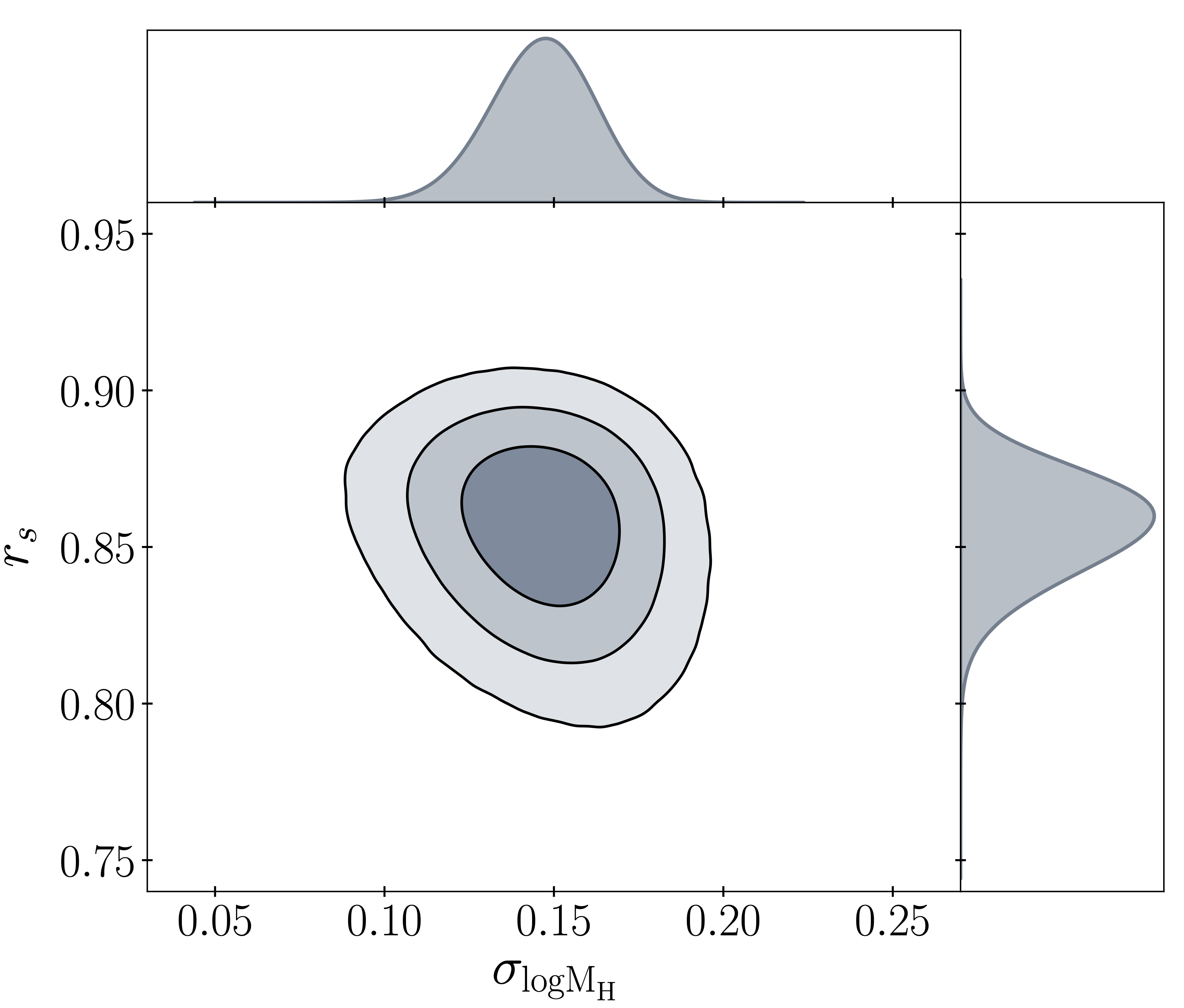
Figure 4: Posterior distribution (1$\sigma$, 2$\sigma$, 3$\sigma$ contours) of the model that fits for variations in galaxy number density within the SHMR for red central galaxies. The x-axis shows the random error in the halo mass estimates from the group catalog. The y-axis shows the Spearman’s rank correlation coefficient between $\mathrm{t}_{\mathrm{halo}}$ and M_∗ at fixed M_H (i.e., the galaxy assembly bias signal). The no-correlation case corresponds to $r_{s}=0$ and the perfect correlation case corresponds to $r_{s}=1$. The absence of assembly bias ($r_{s}=0$) is inconsistent with the data.

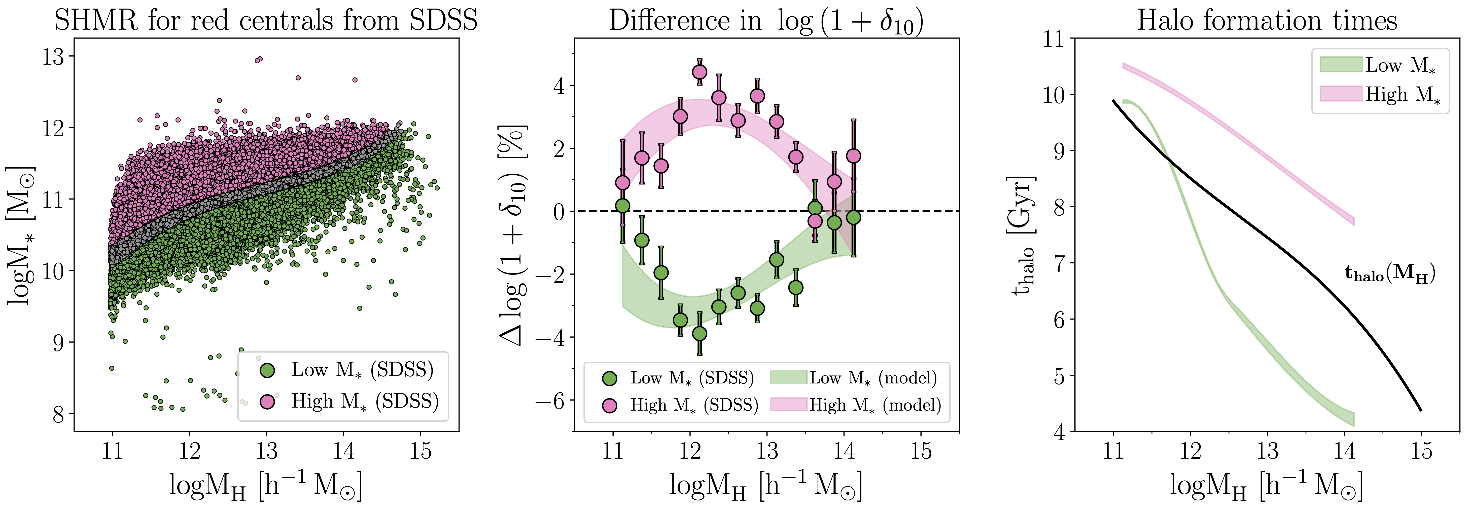
Figure 5: Model solution after convergence. Left: The SHMR for red central galaxies from SDSS highlighting the two subsamples (same as Figure 1). High-M_∗ centrals are plotted in magenta ($>66$th percentile in the SHMR) and low-M_∗ centrals are plotted in green ($<33$rd percentile in the SHMR). Middle: Difference in galaxy number density within $R=10~{}h^{-1}$ Mpc between high- and low-M_∗ red centrals as a function of M_H (datapoints). The shaded regions show the 1$\sigma$ difference in galaxy number density from a random sampling of the converged posterior. Right: 1$\sigma$ intervals of the $\mathrm{t}_{\mathrm{halo}}$ of high-M_∗ and low-M_∗ red centrals as constrained by the model. Also shown in black is the median $\mathrm{t}_{\mathrm{halo}}$ of host halos in the MDPL2 simulation as a function of M_H. Note that the average between the $\mathrm{t}_{\mathrm{halo}}$ of high-M_∗ and low-M_∗ red centrals differs from the median $\mathrm{t}_{\mathrm{halo}}$ in MDPL2 because the median $\mathrm{t}_{\mathrm{halo}}$ was computed for all centrals (i.e., both red and blue).

4 Results

Plotted in the top left panel of Figure 2 is the SHMR for red central galaxies from SDSS separated into two bins of M_∗ at fixed M_H (Section 3.1). The bottom left panel shows that centrals with high-M_∗ have systematically higher galaxy number densities within $R=10~{}h^{-1}$ Mpc than centrals with low-M_∗, especially in the M_H range between $10^{11.5}-10^{13.5}~{}h^{-1}$ M_⊙. This result is evidence that the M_∗ of galaxies vary with the density of the large scale structure at fixed M_H.

We can confirm that this result holds true after controlling for all three quantities involved in the measurement. Upon substitution of M_H with group r-band luminosity and M_∗ with central galaxy r-band luminosity, differences in $\delta_{10}$ remain significant (middle panel of Figure 2). We also controlled for $\delta_{10}$ by utilizing reconstructions of the Cosmic Web with the Monte Carlo Physarum Machine (MCPM) Slime Mold algorithm (Burchett et al. 2020). In contrast to the number density of galaxies, which is sensitive to the abundance of luminous matter in the large scale structure, the MCPM Slime Mold catalog (Wilde et al. 2023) provides estimates for the density field in its totality, including dark-matter (Hasan et al. 2023a). This was achieved through the adaptation of an algorithm designed to characterize the growth of ‘slime mold’, enabling reconstruction of the tri-dimensional structure of the Cosmic Web. We used the publicly available measurements in replacement of the number density of galaxies, achieving a consistent — and perhaps even more significant — signal in the right panel of Figure 2. Taken together, these results are evidence that the baryonic properties of central galaxies correlate with the density of the large scale structure after controlling for the mass at the halo scale.

While differences in $\delta_{10}$ are suggestive of differences in halo formation time (e.g. Lee et al. 2017; Alpaslan & Tinker 2020), modeling is required in order to account for other possible sources of variation in $\delta_{10}$. The framework introduced in Section 3.2 serves this purpose by simultaneously modeling the effects of M_H errors and galaxy assembly bias on $\delta_{10}$ variations within the red SHMR. We fitted this model to the observed differences in $\delta_{10}$ (left panel of Figure 2) and obtained the posterior distribution shown in Figure 4. Inspection of this figure reveals that random errors in the halo mass estimates and a galaxy assembly bias signal are both needed to explain the differences in $\delta_{10}$, with $\sigma_{\log{\mathrm{M}_{\mathrm{H}}}}\sim 0.15$ dex and $r_{s}\sim 0.85$ best reproducing the observations. Errors in the M_H of this magnitude are within expectations from the group finder algorithm ($\sigma_{\log{\mathrm{M}_{\mathrm{H}}}}\lesssim 0.2$; Tinker 2022) and the marginal posterior probability for $r_{s}$ rejects the absence of galaxy assembly bias ($r_{s}=0$) with confidence $>5\sigma$.

The model solutions are plotted along with the data in Figure 5. As revealed by the middle panel, the differences in galaxy number density at fixed M_H are well reproduced by the converged model. Plotted in the right panel are the the halo formation times of low- and high-M_∗ red centrals that have been inferred by our model. More massive dark-matter halos form at later times, and halos that are old for their M_H host galaxies with higher M_∗. We can confirm that this result also holds true for different definitions of halo formation time: at fixed M_H, halos with older $\mathrm{t}_{\mathrm{halo}}^{11.5}$ (as defined in Section 3.1) host higher M_∗ galaxies.

5 Discussion

Variations in the baryonic properties of galaxies at fixed M_H have been observed for a few years (e.g. Oyarzún et al. 2022; Scholz-Díaz et al. 2022, 2023, 2024). However, diagnosing the source of these variations has been difficult due to the stochastic nature of galaxy formation and because of the systematic errors affecting observational halo diagnostics (e.g. Calderon et al. 2018; Tinker et al. 2018). In this context, we have determined that some of these variations at fixed M_H, in particular differences in stellar mass and/or galaxy luminosity, are correlated with how luminous matter is arranged in large ($R=10~{}h^{-1}$ Mpc) scales. In this section, we discuss the biases and/or the underlying physical processes that could be driving this connection.

5.1 Systematic errors in the group catalog

It is important to address how systematic errors in our approach could fabricate a signal in the galaxy number densities. Errors in the halo mass estimates from the group catalog are particularly relevant, which is the reason for their inclusion in the model. As we show in Figure 4, random errors in the group catalog alone cannot explain the differences in galaxy number densities at fixed M_H. That said, should the errors in the group finder not be random (i.e., stellar- or halo-mass dependent), then any signal in the galaxy number densities could be fabricated. For instance, weak-lensing analyses have revealed differences between the underlying M_H distributions of red and blue central galaxies in the Yang et al. (2007) group catalog, indicating that the scatter of the SHMR correlates with the physical properties of galaxies in an unaccounted for manner (Lin et al. 2016).

Our approach accounts for these difficulties in multiple ways. First, our detection is not reliant on differences between red and blue centrals, since the latter were removed from our sample. Second, the impact of the color-dependent spatial distribution of galaxies on halo mass estimation is accounted for, as the Tinker (2022) algorithm is designed to fit for the clustering of red and blue galaxies separately. It is also reassuring that the SDSS implementation of the algorithm can reproduce the weak-lensing derived SHMR (Mandelbaum et al. 2016), especially for red centrals in our M_H regime (Tinker 2021). Finally, the fact that we also recover the signal when using total group luminosity instead of M_H (Figure 2) is an indication that the signal is not fabricated by how the halo masses are assigned by the group finder algorithm.

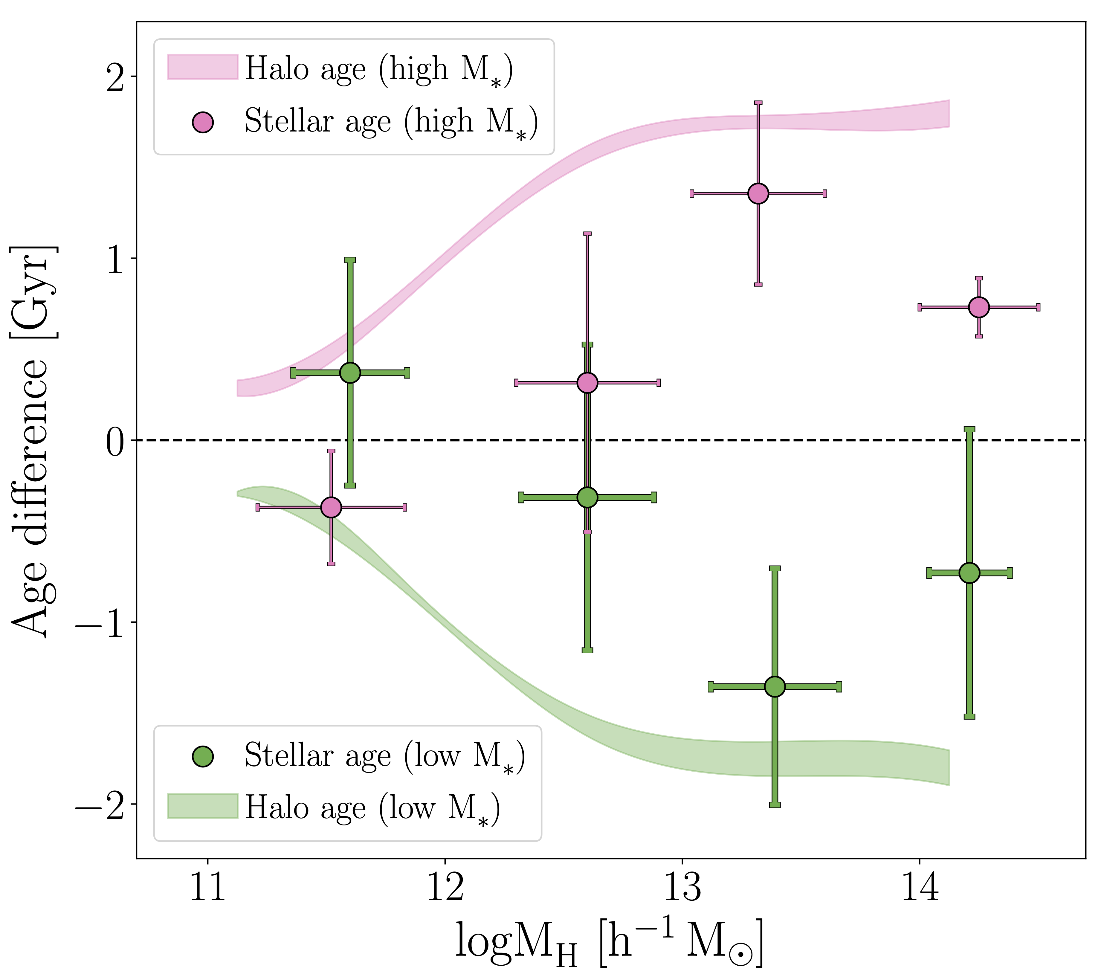
Figure 6: Variations in halo (this work) and galaxy (Oyarzún et al. 2022) formation times within the SHMR for red central galaxies. High- and low-M_∗ centrals were defined according to the 33rd and 66th percentiles in M_∗-to-M_H ratio in the red SHMR (magenta and green, respectively). The differences for both high- and low-M_∗ centrals are relative to the median formation time at a given M_H. The differences in halo formation time correspond to the 1$\sigma$ spread of a random posterior sampling (shaded regions). The differences in galaxy formation time correspond to the average mass-weighted stellar ages derived from stellar population fitting of MaNGA spectra (datapoints). Differences in the formation times are $\sim 1-3$ Gyr for both halos and galaxies.

Systematic errors in group catalogs can also stem from central and satellite galaxy mis-classification. Lin et al. (2016) showed that satellite contamination can affect the correlation functions and the dark matter profiles of central galaxy samples. Yet, as also pointed out by Lin et al. (2016), satellites that are mis-classified as centrals reflect the large-scale bias of their higher M_H hosts. As the normalized densities converge at high M_H (Figure 3), central and satellite galaxy mis-classification would weaken the assembly bias signal; a conclusion that we can confirm applies to our dataset after conducting simulations of galaxy miss-classifications. Moreover, adopting a central selection criterion of P${}_{sat}<0.01$ instead of P${}_{sat}<0.1$ does not impact our results.

Any systematic errors arising from our M_∗ are unlikely. At fixed M_H, the measurement error of our stellar masses is $\Delta$M${}_{*}<0.18$ dex (Tinker et al. 2017), much smaller than the $\sim 0.4$ dex separating our two M_∗ subsamples (left panel of Figure 1). Moreover, the signal is also recovered after substituting M_∗ with L_∗ (Figure 2). The normalized number densities are similarly robust, with the flux limit of the DLIS reaching $22.8$ mag at 5$\sigma$ (Dey et al. 2019), which is $5-6$ magnitudes deeper than the $m_{*}$ of the galaxy luminosity function at $z=0.1$ (Blanton et al. 2005). We also confirm that the signal is recovered with independent metrics for the density of the large scale structure (i.e., the Slime Mold reconstruction of the Cosmic Web; Figure 2).

Still, quantifying the magnitude and significance of galaxy assembly bias with other probes for M_H remains a priority. Weak lensing can be used to search for systematic differences between the total mass surface density profiles of high- and low-M_∗ centrals (e.g. Lin et al. 2016). In addition, host M_H can also be estimated through the tight correlation between central M_∗, M_H, and M${}^{max}_{*}$ (where M${}^{max}_{*}$ is the the stellar mass of the central out to 100 kpc; Huang et al. 2020) or via the stellar-to-total dynamical mass relation for central galaxies (Scholz-Díaz et al. 2024). Also key will be alternative methods for estimating halo formation times in observations (e.g. machine learning algorithms; Lyu et al. 2024).

5.2 Analytic model for galaxy assembly bias

The magnitude of the difference in halo formation time between the two M_∗-selected subsamples that has been inferred by our method is $\sim 1-3$ Gyr (Figure 6). Differences of this magnitude are consistent with the variations in stellar age that we found in Oyarzún et al. (2022, also plotted in Figure 6) after similarly dissecting the red SHMR of nearby galaxies. In an approach that is analogue to that of Section 3.1, we also separated central galaxies according to the 33rd and 66th percentiles in M_∗-to-M_H ratio, recovering variations in the timescales of galaxy formation at fixed M_H that are not drastically different from the variations in the timescales of halo formation. In this subsection, we will show that variations in the stellar ages and stellar masses of galaxies with the large-scale environment (at fixed M_H) can be interpreted as a natural outcome of linear structure-formation theory and the regulation of star-formation through energy-conserving feedback.

We will first discuss the difference in stellar age with galaxy environment in large scales (Figure 6). In this context, $R=10~{}h^{-1}$ Mpc is a natural scale to consider because that is the non-linear mass scale in the local Universe. The redshift at which a particular region of the Universe reaches a virialized or collapsed mass fraction (i.e., M_H) depends on the large scale overdensity, with overdense regions having accelerated structure formation. According to extended Press-Schechter theory, the variance in redshift at which a region of the Universe within a radius $R$ will reach a particular collapsed fraction is

$$\sigma_{z}=\frac{\sigma(R)}{1.69\,(1+z)},$$ (9)

where $\sigma(R)$ is the variance in the density field (Barkana & Loeb 2004; Wyithe & Loeb 2004). For $R=10$ cMpc at $z=0$, the variance in redshift is $\sigma_{z}\approx 0.6$. These variations can be linked to differences in the formation of structure for an overdense Universe, i.e.,

$$dt=\left|\frac{dt}{dz}\right|dz=\frac{\sigma_{z}}{(1+z)\,H(z)}\approx 1~{}\mbox{Gyr at }z=0.$$ (10)

Variations of this magnitude are consistent with the observed differences in age between the stellar populations of galaxies in large scale overdensities and underdensities at fixed M_H (Figure 6).

With this result in hand, we can predict the differences in M_∗ between old and young populations at fixed M_H. Stellar populations with ages of $10$ Gyr formed before quasars were dominant in regulating stellar growth (e.g. Croton et al. 2006a, b). Under the ansatz that stellar growth is set by the balance between the binding energy of the star-forming gas and the mechanical energy from supernovae (the base assumption in almost all semi-analytic models and numerical simulations), the ratio between stellar and halo mass corresponds to

$$\frac{M_{*}}{\mathrm{M}_{\mathrm{H}}}\propto\mathrm{M}_{\mathrm{H}}^{2/3}(1+z),$$ (11)

as in Dekel & Woo (2003) and Wyithe & Loeb (2003). This implies that the range in M_∗ at fixed M_H owing to variations in the formation time is

$$\Delta\mbox{M}_{*}=\frac{(1+z+\sigma_{z})}{(1+z-\sigma_{z})}.$$ (12)

For the derived value of $\sigma_{z}\approx 0.6$ for $R=10$ cMpc, $\Delta\mbox{M}_{*}\approx 3$ for stars forming at $z=0$ and $\Delta\mbox{M}_{*}\approx 2$ for stars forming at $z=1$. These values match the range of stellar mass that separates the high-M_∗ and low-M_∗ subsamples ($\Delta\mbox{logM}_{*}\approx 0.4$; Figure 1).

5.3 Galaxy assembly bias in simulations

The results shown in Figure 5 and the analytical arguments presented in Section 5.2 can be interpreted as an underlying correlation between M_∗ and halo formation time. In this scenario, the properties of galaxies are dependent not only on the masses of dark matter halos, but also on secondary halo properties like formation time or assembly history. A fixed M_H, older halos form deeper gravitational potentials that facilitate the assembly of higher M_∗ central galaxies (e.g. Matthee et al. 2017).

Our model associates variations in $\delta_{10}$ across M${}_{\mathrm{H}}\sim 10^{11}-10^{14}~{}h^{-1}$ M_⊙ with a strong correlation between halo formation time and stellar mass ($r_{s}\sim 0.85$) across this M_H range. In broad agreement with this result, the correlation between halo age and M_∗ is present across the M${}_{\mathrm{H}}\sim 10^{11}-10^{13.5}~{}h^{-1}$ M_⊙ range in the IllustrisTNG simulation (Zehavi et al. 2018; Xu & Zheng 2020). Interestingly, the galaxy assembly bias in IllustrisTNG is also present when using the number density of particles within $R\sim 5~{}h^{-1}$ Mpc instead of $\mathrm{t}_{\mathrm{halo}}$ (Zehavi et al. 2018), which is consistent with our analysis in SDSS (albeit with the considerations regarding the choice of $R$ outlined in Section 3.1).

We note that the magnitude of the $\delta_{10}$ differences peak around M${}_{\mathrm{H}}\sim 10^{12}$ M_⊙. However, because we adopt a constant value for $r_{s}$ across all M_H, we may not interpret any dependence of the $\delta_{10}$ variations on M_H as a signature of a M_H-dependent galaxy assembly bias signal. Some theoretical work — e.g. IllustrisTNG (Vogelsberger et al. 2014; Nelson et al. 2015) — predict the galaxy assembly bias signal to decrease in magnitude toward M${}_{\mathrm{H}}>10^{13.5}~{}h^{-1}$ M_⊙ (Zehavi et al. 2018; Xu & Zheng 2020). On the other hand, galaxy assembly bias remains strong in the UniverseMachine (Behroozi et al. 2019) for M${}_{\mathrm{H}}>10^{14}~{}h^{-1}$ M_⊙ (Bradshaw et al. 2020). The EAGLE simulation (Crain et al. 2015; Schaye et al. 2015) is at the other end of the spectrum, predicting that halo formation time has little impact above M${}_{\mathrm{H}}\gtrsim 10^{11.5}~{}h^{-1}$ M_⊙ (Matthee et al. 2017).

Some of the discrepancy between these simulations may originate in how halo and galaxy mergers are handled, especially given that mergers become increasingly important as M_H increases (Huang et al. 2013a, b, 2018, 2020; Oyarzún et al. 2019; Angeloudi et al. 2024). In the case of our work, this is apparent in the little sensitivity of $\delta_{10}$ variations to the correlation between $\mathrm{t}_{\mathrm{halo}}$ and M_∗ toward M${}_{\mathrm{H}}>10^{13.5}~{}h^{-1}$ M_⊙ (Figure 4). This justifies the choice of fitting for a single, M_H-independent value for $r_{s}$, and it ultimately stems from how $\mathrm{t}_{\mathrm{halo}}$ and $\delta_{10}$ are correlated at these M_H in MDPL2.

For a more quantitative comparison with simulations, we can turn to $r_{s}$. We are particularly interested in comparing our recovered value of $r_{s}\sim 0.85$ — which is indicative of a strong correlation between $\mathrm{t}_{\mathrm{halo}}$ and M_∗ at fixed M_H — with expectations from semi-empirical models. For this purpose, we analyzed data for the SHMR from the UniverseMachine. We calculated $\mathrm{t}_{\mathrm{halo}}$ following the same definition outlined in Section 3.1 and computed $r_{s}$ between $\mathrm{t}_{\mathrm{halo}}$ and M_∗ at fixed M_H. We found $r_{s}$ to peak at M${}_{\mathrm{H}}\sim 10^{11}-10^{12}~{}h^{-1}$ M_⊙ with values of $r_{s}\sim 0.5-0.6$. We conclude that semi-empirical models like the UniverseMachine predict a correlation between $\mathrm{t}_{\mathrm{halo}}$ and M_∗ that is only slightly weaker than what we inferred from SDSS.

So far, we have discussed how variations in halo formation time can affect the M_∗ (this work) and stellar ages (Oyarzún et al. 2022) of central galaxies (Figure 6). We should highlight that the stellar population variations that we identified in Oyarzún et al. (2022) also extend to chemical content of galaxies. Besides being older, centrals with high M_∗-to-M_H ratios also feature low [Fe/H] and high [Mg/Fe]. The natural interpretation for these trends is that centrals with high-M_∗ for their M_H not only form their stars early, but that they also assemble them in rapid timescales, resulting in high [$\alpha$/Fe] (e.g. Faber & Jackson 1976; Faber et al. 1985; Thomas et al. 2005). Variations in the star-formation timescale may also be connected with variations in secondary halo properties, in particular with halo formation time and halo concentration. At fixed M_H, older and higher-concentration halos are thought to bind the stellar and gaseous contents of centrals more strongly (e.g. Wechsler et al. 2002; Hearin et al. 2016). These results — along with the work by Winkel et al. (2021); Donnan et al. (2022); Zhou et al. (2024) — provide tentative observational evidence for a correlation between secondary halo properties and the quenching epochs and the metal content in galaxies (as seen in simulations; e.g. Booth & Schaye 2010; Matthee et al. 2017; Montero-Dorta et al. 2020, 2021; Hasan et al. 2023b).

Our studies of how $\delta_{10}$ and the stellar populations of galaxies vary within the SHMR were in great part enabled by publicly available datasets of high statistical power (i.e., SDSS and MaNGA). SDSS is the largest publicly available spectroscopic survey of galaxies in the nearby Universe, providing the necessary statistics for dissecting the SHMR, the required spectra for accurately measuring stellar masses, and the deep ancillary imaging needed for precise estimation of the halo mass. At the same time, MaNGA is the largest spatially resolved spectroscopic survey of nearby galaxies. In terms of spectroscopic constraining power, MaNGA surpasses even SDSS (see Oyarzún et al. 2022), allowing for the most precise measurements of stellar age and chemical abundances possible in the SHMR of nearby galaxies. This will soon change, with surveys like the Bright Galaxy Sample of the DESI Experiment (DESI Collaboration et al. 2016) spearheading the next generation of datasets that will enable detailed characterization of the galaxy-halo connection at low redshifts.

6 Summary

We used the group catalog from Tinker (2021, 2022) to study the stellar-to-halo mass relation for red central galaxies from SDSS across the halo mass range M${}_{\mathrm{H}}=10^{11}-10^{15}~{}h^{-1}$ M_⊙. We showed that the stellar masses of red central galaxies vary not only with the mass of the dark-matter halo, but also with the number density of galaxies in large scales ($R=10~{}h^{-1}$ Mpc). Our preferred interpretation for this result is that the stellar masses of central galaxies depend on both halo mass and halo formation time. This interpretation is motivated by our current cosmological picture, in which high density regions of the large scale structure assemble earlier in cosmic history.

To quantify the relation between the large-scale number density of galaxies and their halo formation time, we exploited the MDPL2 dark-matter-only cosmological simulation (Prada et al. 2012). With the halo formation times in hand, we constructed a model that reproduces differences in the observed number density of galaxies via two parameters: (1) random errors in the halo masses estimated by the group catalog and (2) the correlation between halo formation time and stellar mass at fixed halo mass (i.e., the galaxy assembly bias signal). We quantified the model posterior with SDSS and found that errors in the halo masses from the group catalog are $\sim 0.15$ dex (in agreement with the expected $\lesssim 0.2$ dex errors from the group finder algorithm; Tinker 2022) and that galaxy assembly bias is necessary for explaining our results at $>5\sigma$ significance.

Our best-fit model indicates that variations in the stellar masses of red central galaxies at fixed halo mass correlate with differences in halo formation time of $\sim 1-3$ Gyr. Differences of this magnitude are remarkably consistent with differences in the star-formation histories of galaxies at fixed halo mass, which we measured previously in Oyarzún et al. (2022). Taken together, these results are indicative that old halos (at fixed halo mass) are associated with more massive, older, and more rapidly assembled central galaxies.

We also considered how systematic errors in the group finder algorithm could fabricate the signal that we observe in the galaxy number densities. While systematic and random errors are likely present, they alone cannot reproduce the signal. This is because we still detect a similarly significant difference in the galaxy number densities after substituting M_H for total group luminosity and M_∗ for galaxy luminosity.

7 Data Availability

Underlying data in this article will be shared upon reasonable request to the corresponding author.

We thank the reviewer of this paper for their insightful comments and suggestions. G.O. acknowledges support by the National Science Foundation through grants AST-2107989 and AST-2107990. This work made use of Astropy, a community-developed core Python package and an ecosystem of tools and resources for astronomy (Astropy Collaboration et al., 2013, 2018, 2022). Funding for the Sloan Digital Sky Survey (SDSS) has been provided by the Alfred P. Sloan Foundation, the Participating Institutions, the National Aeronautics and Space Administration, the National Science Foundation, the U.S. Department of Energy, the Japanese Monbukagakusho, and the Max Planck Society. The SDSS Web site is http://www.sdss.org/. The SDSS is managed by the Astrophysical Research Consortium (ARC) for the Participating Institutions. The Participating Institutions are The University of Chicago, Fermilab, the Institute for Advanced Study, the Japan Participation Group, The Johns Hopkins University, Los Alamos National Laboratory, the Max-Planck-Institute for Astronomy (MPIA), the Max-Planck-Institute for Astrophysics (MPA), New Mexico State University, University of Pittsburgh, Princeton University, the United States Naval Observatory, and the University of Washington. The MultiDark Database used in this paper and the web application providing online access to it were constructed as part of the activities of the German Astrophysical Virtual Observatory as result of a collaboration between the Leibniz-Institute for Astrophysics Potsdam (AIP) and the Spanish MultiDark Consolider Project CSD2009-00064. The Bolshoi and MultiDark simulations were run on the NASA’s Pleiades supercomputer at the NASA Ames Research Center. The MultiDark-Planck (MDPL) and the BigMD simulation suite have been performed in the Supermuc supercomputer at LRZ using time granted by PRACE.

References

- Aihara et al. (2011) Aihara, H., Allende Prieto, C., An, D., et al. 2011, ApJS, 193, 29, doi: 10.1088/0067-0049/193/2/29
- Alam et al. (2015) Alam, S., Albareti, F. D., Allende Prieto, C., et al. 2015, ApJS, 219, 12, doi: 10.1088/0067-0049/219/1/12
- Alpaslan & Tinker (2020) Alpaslan, M., & Tinker, J. L. 2020, MNRAS, 496, 5463, doi: 10.1093/mnras/staa1844
- Angeloudi et al. (2024) Angeloudi, E., Falcón-Barroso, J., Huertas-Company, M., et al. 2024, arXiv e-prints, arXiv:2407.00166, doi: 10.48550/arXiv.2407.00166
- Astropy Collaboration et al. (2013) Astropy Collaboration, Robitaille, T. P., Tollerud, E. J., et al. 2013, A&A, 558, A33, doi: 10.1051/0004-6361/201322068
- Astropy Collaboration et al. (2018) Astropy Collaboration, Price-Whelan, A. M., Sipőcz, B. M., et al. 2018, AJ, 156, 123, doi: 10.3847/1538-3881/aabc4f
- Astropy Collaboration et al. (2022) Astropy Collaboration, Price-Whelan, A. M., Lim, P. L., et al. 2022, ApJ, 935, 167, doi: 10.3847/1538-4357/ac7c74
- Barkana & Loeb (2004) Barkana, R., & Loeb, A. 2004, ApJ, 609, 474, doi: 10.1086/421079
- Behroozi et al. (2019) Behroozi, P., Wechsler, R. H., Hearin, A. P., & Conroy, C. 2019, MNRAS, 488, 3143, doi: 10.1093/mnras/stz1182
- Blanton et al. (2005) Blanton, M. R., Eisenstein, D., Hogg, D. W., Schlegel, D. J., & Brinkmann, J. 2005, ApJ, 629, 143, doi: 10.1086/422897
- Blumenthal et al. (1984) Blumenthal, G. R., Faber, S. M., Primack, J. R., & Rees, M. J. 1984, Nature, 311, 517, doi: 10.1038/311517a0
- Booth & Schaye (2010) Booth, C. M., & Schaye, J. 2010, MNRAS, 405, L1, doi: 10.1111/j.1745-3933.2010.00832.x
- Bradshaw et al. (2020) Bradshaw, C., Leauthaud, A., Hearin, A., Huang, S., & Behroozi, P. 2020, MNRAS, 493, 337, doi: 10.1093/mnras/staa081
- Brinchmann et al. (2004) Brinchmann, J., Charlot, S., White, S. D. M., et al. 2004, MNRAS, 351, 1151, doi: 10.1111/j.1365-2966.2004.07881.x
- Bundy et al. (2015) Bundy, K., Bershady, M. A., Law, D. R., et al. 2015, ApJ, 798, 7, doi: 10.1088/0004-637X/798/1/7
- Burchett et al. (2020) Burchett, J. N., Elek, O., Tejos, N., et al. 2020, ApJ, 891, L35, doi: 10.3847/2041-8213/ab700c
- Calderon et al. (2018) Calderon, V. F., Berlind, A. A., & Sinha, M. 2018, MNRAS, 480, 2031, doi: 10.1093/mnras/sty2000
- Campbell et al. (2015) Campbell, D., van den Bosch, F. C., Hearin, A., et al. 2015, MNRAS, 452, 444, doi: 10.1093/mnras/stv1091
- Chen et al. (2012) Chen, Y.-M., Kauffmann, G., Tremonti, C. A., et al. 2012, MNRAS, 421, 314, doi: 10.1111/j.1365-2966.2011.20306.x
- Cortese et al. (2019) Cortese, L., van de Sande, J., Lagos, C. P., et al. 2019, MNRAS, 485, 2656, doi: 10.1093/mnras/stz485
- Crain et al. (2015) Crain, R. A., Schaye, J., Bower, R. G., et al. 2015, MNRAS, 450, 1937, doi: 10.1093/mnras/stv725
- Croton et al. (2007) Croton, D. J., Gao, L., & White, S. D. M. 2007, MNRAS, 374, 1303, doi: 10.1111/j.1365-2966.2006.11230.x
- Croton et al. (2006a) Croton, D. J., Springel, V., White, S. D. M., et al. 2006a, MNRAS, 365, 11, doi: 10.1111/j.1365-2966.2005.09675.x
- Croton et al. (2006b) —. 2006b, MNRAS, 367, 864, doi: 10.1111/j.1365-2966.2006.09994.x
- Dawson et al. (2013) Dawson, K. S., Schlegel, D. J., Ahn, C. P., et al. 2013, AJ, 145, 10, doi: 10.1088/0004-6256/145/1/10
- Dekel & Woo (2003) Dekel, A., & Woo, J. 2003, MNRAS, 344, 1131, doi: 10.1046/j.1365-8711.2003.06923.x
- DESI Collaboration et al. (2016) DESI Collaboration, Aghamousa, A., Aguilar, J., et al. 2016, arXiv e-prints, arXiv:1611.00036. https://arxiv.org/abs/1611.00036
- Dey et al. (2019) Dey, A., Schlegel, D. J., Lang, D., et al. 2019, AJ, 157, 168, doi: 10.3847/1538-3881/ab089d
- Donnan et al. (2022) Donnan, C. T., Tojeiro, R., & Kraljic, K. 2022, Nature Astronomy, 6, 599, doi: 10.1038/s41550-022-01619-w
- Faber et al. (1985) Faber, S. M., Friel, E. D., Burstein, D., & Gaskell, C. M. 1985, ApJS, 57, 711, doi: 10.1086/191024
- Faber & Jackson (1976) Faber, S. M., & Jackson, R. E. 1976, ApJ, 204, 668, doi: 10.1086/154215
- Foreman-Mackey et al. (2013) Foreman-Mackey, D., Hogg, D. W., Lang, D., & Goodman, J. 2013, PASP, 125, 306, doi: 10.1086/670067
- Gallazzi et al. (2020) Gallazzi, A. R., Pasquali, A., Zibetti, S., & La Barbera, F. 2020, arXiv e-prints, arXiv:2010.04733. https://arxiv.org/abs/2010.04733
- Gao et al. (2005) Gao, L., Springel, V., & White, S. D. M. 2005, MNRAS, 363, L66, doi: 10.1111/j.1745-3933.2005.00084.x
- Gunn et al. (2006) Gunn, J. E., Siegmund, W. A., Mannery, E. J., et al. 2006, AJ, 131, 2332, doi: 10.1086/500975
- Hadzhiyska et al. (2021) Hadzhiyska, B., Bose, S., Eisenstein, D., & Hernquist, L. 2021, MNRAS, 501, 1603, doi: 10.1093/mnras/staa3776
- Hadzhiyska et al. (2023) Hadzhiyska, B., Eisenstein, D., Hernquist, L., et al. 2023, MNRAS, 524, 2507, doi: 10.1093/mnras/stad731
- Hahn et al. (2007) Hahn, O., Porciani, C., Carollo, C. M., & Dekel, A. 2007, MNRAS, 375, 489, doi: 10.1111/j.1365-2966.2006.11318.x
- Hasan et al. (2023a) Hasan, F., Burchett, J. N., Hellinger, D., et al. 2023a, arXiv e-prints, arXiv:2311.01443, doi: 10.48550/arXiv.2311.01443
- Hasan et al. (2023b) Hasan, F., Burchett, J. N., Abeyta, A., et al. 2023b, ApJ, 950, 114, doi: 10.3847/1538-4357/acd11c
- Hearin et al. (2016) Hearin, A. P., Zentner, A. R., van den Bosch, F. C., Campbell, D., & Tollerud, E. 2016, MNRAS, 460, 2552, doi: 10.1093/mnras/stw840
- Huang et al. (2013a) Huang, S., Ho, L. C., Peng, C. Y., Li, Z.-Y., & Barth, A. J. 2013a, ApJ, 766, 47, doi: 10.1088/0004-637X/766/1/47
- Huang et al. (2013b) —. 2013b, ApJ, 768, L28, doi: 10.1088/2041-8205/768/2/L28
- Huang et al. (2018) Huang, S., Leauthaud, A., Greene, J. E., et al. 2018, MNRAS, 475, 3348, doi: 10.1093/mnras/stx3200
- Huang et al. (2020) Huang, S., Leauthaud, A., Hearin, A., et al. 2020, MNRAS, 492, 3685, doi: 10.1093/mnras/stz3314
- Kauffmann (2015) Kauffmann, G. 2015, MNRAS, 454, 1840, doi: 10.1093/mnras/stv2113
- Kauffmann et al. (2013) Kauffmann, G., Li, C., Zhang, W., & Weinmann, S. 2013, MNRAS, 430, 1447, doi: 10.1093/mnras/stt007
- Klypin et al. (2016) Klypin, A., Yepes, G., Gottlöber, S., Prada, F., & Heß, S. 2016, MNRAS, 457, 4340, doi: 10.1093/mnras/stw248
- Kravtsov et al. (2004) Kravtsov, A. V., Berlind, A. A., Wechsler, R. H., et al. 2004, ApJ, 609, 35, doi: 10.1086/420959
- Kroupa (2001) Kroupa, P. 2001, MNRAS, 322, 231, doi: 10.1046/j.1365-8711.2001.04022.x
- Lacerna et al. (2022) Lacerna, I., Rodriguez, F., Montero-Dorta, A. D., et al. 2022, MNRAS, 513, 2271, doi: 10.1093/mnras/stac1020
- Lee et al. (2017) Lee, C. T., Primack, J. R., Behroozi, P., et al. 2017, MNRAS, 466, 3834, doi: 10.1093/mnras/stw3348
- Lehmann et al. (2017) Lehmann, B. V., Mao, Y.-Y., Becker, M. R., Skillman, S. W., & Wechsler, R. H. 2017, ApJ, 834, 37, doi: 10.3847/1538-4357/834/1/37
- Lemson & Kauffmann (1999) Lemson, G., & Kauffmann, G. 1999, MNRAS, 302, 111, doi: 10.1046/j.1365-8711.1999.02090.x
- Li et al. (2008) Li, Y., Mo, H. J., & Gao, L. 2008, MNRAS, 389, 1419, doi: 10.1111/j.1365-2966.2008.13667.x
- Lin et al. (2016) Lin, Y.-T., Mandelbaum, R., Huang, Y.-H., et al. 2016, ApJ, 819, 119, doi: 10.3847/0004-637X/819/2/119
- Ludlow et al. (2014) Ludlow, A. D., Navarro, J. F., Angulo, R. E., et al. 2014, MNRAS, 441, 378, doi: 10.1093/mnras/stu483
- Lyu et al. (2024) Lyu, C., Peng, Y., Jing, Y., et al. 2024, arXiv e-prints, arXiv:2407.03409. https://arxiv.org/abs/2407.03409
- Mandelbaum et al. (2016) Mandelbaum, R., Wang, W., Zu, Y., et al. 2016, MNRAS, 457, 3200, doi: 10.1093/mnras/stw188
- Mansfield & Kravtsov (2020) Mansfield, P., & Kravtsov, A. V. 2020, MNRAS, 493, 4763, doi: 10.1093/mnras/staa430
- Mao et al. (2017) Mao, Y.-Y., Zentner, A. R., & Wechsler, R. H. 2017, ArXiv e-prints. https://arxiv.org/abs/1705.03888
- Maraston & Strömbäck (2011) Maraston, C., & Strömbäck, G. 2011, MNRAS, 418, 2785, doi: 10.1111/j.1365-2966.2011.19738.x
- Matthee et al. (2017) Matthee, J., Schaye, J., Crain, R. A., et al. 2017, MNRAS, 465, 2381, doi: 10.1093/mnras/stw2884
- Mo & White (1996) Mo, H. J., & White, S. D. M. 1996, MNRAS, 282, 347, doi: 10.1093/mnras/282.2.347
- Montero-Dorta et al. (2021) Montero-Dorta, A. D., Chaves-Montero, J., Artale, M. C., & Favole, G. 2021, arXiv e-prints, arXiv:2105.05274. https://arxiv.org/abs/2105.05274
- Montero-Dorta & Rodriguez (2024) Montero-Dorta, A. D., & Rodriguez, F. 2024, MNRAS, doi: 10.1093/mnras/stae796
- Montero-Dorta et al. (2017) Montero-Dorta, A. D., Pérez, E., Prada, F., et al. 2017, ApJ, 848, L2, doi: 10.3847/2041-8213/aa8cc5
- Montero-Dorta et al. (2020) Montero-Dorta, A. D., Artale, M. C., Abramo, L. R., et al. 2020, MNRAS, 496, 1182, doi: 10.1093/mnras/staa1624
- Moster et al. (2013) Moster, B. P., Naab, T., & White, S. D. M. 2013, MNRAS, 428, 3121, doi: 10.1093/mnras/sts261
- Nelson et al. (2015) Nelson, D., Pillepich, A., Genel, S., et al. 2015, Astronomy and Computing, 13, 12, doi: 10.1016/j.ascom.2015.09.003
- Obuljen et al. (2020) Obuljen, A., Percival, W. J., & Dalal, N. 2020, J. Cosmology Astropart. Phys, 2020, 058, doi: 10.1088/1475-7516/2020/10/058
- Oke & Gunn (1983) Oke, J. B., & Gunn, J. E. 1983, ApJ, 266, 713, doi: 10.1086/160817
- Oyarzún et al. (2023) Oyarzún, G. A., Bundy, K., Westfall, K. B., et al. 2023, ApJ, 947, 13, doi: 10.3847/1538-4357/acbbca
- Oyarzún et al. (2019) —. 2019, ApJ, 880, 111, doi: 10.3847/1538-4357/ab297c
- Oyarzún et al. (2022) —. 2022, ApJ, 933, 88, doi: 10.3847/1538-4357/ac7048
- Pasquali et al. (2010) Pasquali, A., Gallazzi, A., Fontanot, F., et al. 2010, MNRAS, 407, 937, doi: 10.1111/j.1365-2966.2010.17074.x
- Pearl et al. (2023) Pearl, A. N., Zentner, A. R., Newman, J. A., et al. 2023, arXiv e-prints, arXiv:2309.08675, doi: 10.48550/arXiv.2309.08675
- Peng et al. (2012) Peng, Y.-j., Lilly, S. J., Renzini, A., & Carollo, M. 2012, ApJ, 757, 4, doi: 10.1088/0004-637X/757/1/4
- Prada et al. (2012) Prada, F., Klypin, A. A., Cuesta, A. J., Betancort-Rijo, J. E., & Primack, J. 2012, MNRAS, 423, 3018, doi: 10.1111/j.1365-2966.2012.21007.x
- Schaye et al. (2015) Schaye, J., Crain, R. A., Bower, R. G., et al. 2015, MNRAS, 446, 521, doi: 10.1093/mnras/stu2058
- Scholz-Díaz et al. (2022) Scholz-Díaz, L., Martín-Navarro, I., & Falcón-Barroso, J. 2022, MNRAS, 511, 4900, doi: 10.1093/mnras/stac361
- Scholz-Díaz et al. (2023) —. 2023, MNRAS, 518, 6325, doi: 10.1093/mnras/stac3422
- Scholz-Díaz et al. (2024) Scholz-Díaz, L., Martín-Navarro, I., Falcón-Barroso, J., Lyubenova, M., & van de Ven, G. 2024, Nature Astronomy, doi: 10.1038/s41550-024-02209-8
- Sin et al. (2017) Sin, L. P. T., Lilly, S. J., & Henriques, B. M. B. 2017, MNRAS, 471, 1192, doi: 10.1093/mnras/stx1674
- Sunayama et al. (2016) Sunayama, T., Hearin, A. P., Padmanabhan, N., & Leauthaud, A. 2016, MNRAS, 458, 1510, doi: 10.1093/mnras/stw332
- Thomas et al. (2005) Thomas, D., Maraston, C., Bender, R., & Mendes de Oliveira, C. 2005, ApJ, 621, 673, doi: 10.1086/426932
- Tinker (2021) Tinker, J. L. 2021, ApJ, 923, 154, doi: 10.3847/1538-4357/ac2aaa
- Tinker (2022) —. 2022, AJ, 163, 126, doi: 10.3847/1538-3881/ac37bb
- Tinker et al. (2008) Tinker, J. L., Conroy, C., Norberg, P., et al. 2008, ApJ, 686, 53, doi: 10.1086/589983
- Tinker et al. (2018) Tinker, J. L., Hahn, C., Mao, Y.-Y., Wetzel, A. R., & Conroy, C. 2018, MNRAS, 477, 935, doi: 10.1093/mnras/sty666
- Tinker et al. (2017) Tinker, J. L., Brownstein, J. R., Guo, H., et al. 2017, ApJ, 839, 121, doi: 10.3847/1538-4357/aa6845
- Tojeiro et al. (2017) Tojeiro, R., Eardley, E., Peacock, J. A., et al. 2017, MNRAS, 470, 3720, doi: 10.1093/mnras/stx1466
- Vogelsberger et al. (2020) Vogelsberger, M., Marinacci, F., Torrey, P., & Puchwein, E. 2020, Nature Reviews Physics, 2, 42, doi: 10.1038/s42254-019-0127-2
- Vogelsberger et al. (2014) Vogelsberger, M., Genel, S., Springel, V., et al. 2014, MNRAS, 444, 1518, doi: 10.1093/mnras/stu1536
- Wang et al. (2022) Wang, K., Mao, Y.-Y., Zentner, A. R., et al. 2022, MNRAS, 516, 4003, doi: 10.1093/mnras/stac2465
- Wechsler et al. (2002) Wechsler, R. H., Bullock, J. S., Primack, J. R., Kravtsov, A. V., & Dekel, A. 2002, ApJ, 568, 52, doi: 10.1086/338765
- Wechsler & Tinker (2018) Wechsler, R. H., & Tinker, J. L. 2018, ARA&A, 56, 435, doi: 10.1146/annurev-astro-081817-051756
- Wechsler et al. (2006) Wechsler, R. H., Zentner, A. R., Bullock, J. S., Kravtsov, A. V., & Allgood, B. 2006, ApJ, 652, 71, doi: 10.1086/507120
- Weinmann et al. (2006) Weinmann, S. M., van den Bosch, F. C., Yang, X., & Mo, H. J. 2006, MNRAS, 366, 2, doi: 10.1111/j.1365-2966.2005.09865.x
- Wetzel et al. (2013) Wetzel, A. R., Tinker, J. L., Conroy, C., & van den Bosch, F. C. 2013, MNRAS, 432, 336, doi: 10.1093/mnras/stt469
- White & Rees (1978) White, S. D. M., & Rees, M. J. 1978, MNRAS, 183, 341, doi: 10.1093/mnras/183.3.341
- Wilde et al. (2023) Wilde, M. C., Elek, O., Burchett, J. N., et al. 2023, arXiv e-prints, arXiv:2301.02719, doi: 10.48550/arXiv.2301.02719
- Winkel et al. (2021) Winkel, N., Pasquali, A., Kraljic, K., et al. 2021, MNRAS, 505, 4920, doi: 10.1093/mnras/stab1562
- Wyithe & Loeb (2003) Wyithe, J. S. B., & Loeb, A. 2003, ApJ, 595, 614, doi: 10.1086/377475
- Wyithe & Loeb (2004) —. 2004, Nature, 432, 194, doi: 10.1038/nature03033
- Xu & Zheng (2020) Xu, X., & Zheng, Z. 2020, MNRAS, 492, 2739, doi: 10.1093/mnras/staa009
- Yang et al. (2007) Yang, X., Mo, H. J., van den Bosch, F. C., et al. 2007, ApJ, 671, 153, doi: 10.1086/522027
- York et al. (2000) York, D. G., Adelman, J., Anderson, Jr., J. E., et al. 2000, AJ, 120, 1579, doi: 10.1086/301513
- Yuan et al. (2021) Yuan, S., Hadzhiyska, B., Bose, S., Eisenstein, D. J., & Guo, H. 2021, MNRAS, 502, 3582, doi: 10.1093/mnras/stab235
- Zehavi et al. (2018) Zehavi, I., Contreras, S., Padilla, N., et al. 2018, ApJ, 853, 84, doi: 10.3847/1538-4357/aaa54a
- Zehavi et al. (2019) Zehavi, I., Kerby, S. E., Contreras, S., et al. 2019, ApJ, 887, 17, doi: 10.3847/1538-4357/ab4d4d
- Zentner et al. (2019) Zentner, A. R., Hearin, A., van den Bosch, F. C., Lange, J. U., & Villarreal, A. 2019, MNRAS, 485, 1196, doi: 10.1093/mnras/stz470
- Zentner et al. (2014) Zentner, A. R., Hearin, A. P., & van den Bosch, F. C. 2014, MNRAS, 443, 3044, doi: 10.1093/mnras/stu1383
- Zhou et al. (2024) Zhou, S., Aragón-Salamanca, A., & Merrifield, M. 2024, arXiv e-prints, arXiv:2404.16181, doi: 10.48550/arXiv.2404.16181