Spherical Evolution of the Generalized Harmonic Gauge Formulation of General Relativity on Compactified Hyperboloidal Slices

Abstract

We report on the successful numerical evolution of the compactified hyperboloidal initial value problem in general relativity using generalized harmonic gauge. We work in spherical symmetry, using a massless scalar field to drive dynamics. Our treatment is based on the dual-foliation approach, proceeding either by using a height function or by solving the eikonal equation to map between frames. Both are tested here with a naive implementation and with hyperboloidal layers. We present a broad suite of numerical evolutions, including pure gauge perturbations, constraint violating and satisfying data with and without scalar field matter. We present calculations of spacetimes with a regular center. For black hole spacetimes we use excision to remove part of the black hole interior. We demonstrate both pointwise and norm convergence at the expected rate of our discretization. We present evolutions in which the scalar field collapses to form a black hole. Evolving nonlinear scalar field perturbations of the Schwarzschild spacetime, we recover the expected quasinormal frequencies and tail decay rates from linear theory.

I Introduction

Asymptotic flatness is the natural assumption under which to model isolated systems in general relativity (GR) [1]. It may be formalized in a variety of ways, but common to all is the existence of a region far from the ‘center’ in which the metric becomes ever closer to that of the Minkowski spacetime. This leads to the definition of future null infinity, $\mathscr{I}^{+}$, which can be thought of as the collection of endpoints of future directed null geodesics within this asymptotic region. Future null infinity is crucial in various mathematical definitions and, crucially for astrophysics, is the place where gravitational waves (GW) can be unambiguously defined. It is therefore of vital importance to numerical relativity (NR) to have access to it.

The most common approach used in NR is to solve the Einstein field equations (EFEs) in a truncated domain with a timelike outer boundary, evaluating an approximation to outgoing waves on a set of concentric spheres and then extrapolate this data to infinity at fixed retarded time. Eventually waves computed in this way will be affected by artificial boundary conditions. There are however several proposals to include $\mathscr{I}^{+}$ within the computational domain directly. One popular suggestion is to solve the field equations on compactified outgoing null-slices. Depending on whether or not data from the characteristic domain couples back to the method used to treat the central region, this is called either Cauchy-Characteristic-Matching (CCM) or Cauchy-Characteristic-Extraction (CCE). For details see the review [2]. Recent numerical work can be found in [3, 4, 5]. Well-posedness and numerical convergence analysis of CCE and CCM setups in Bondi-like gauges can be found in [6, 7, 8, 9].

Another proposal, pioneered by Friedrich [10, 11, 12], is to foliate spacetime via hyperboloidal slices. These are by definition spacelike hypersurfaces that terminate at null infinity rather than spatial infinity like Cauchy slices. For numerical applications hyperboloidal slices can be combined with a compactified radial coordinate. Following [13] this strategy is now completely standard for perturbative work in a range of applications, see for instance [14, 15, 16]. The essential subtlety in working with compactified coordinates, which do the work of bringing $\mathscr{I}^{+}$ to a finite coordinate distance, is that they introduce divergent quantities into the problem. Fortunately in the asymptotically flat setting these can be off-set by the smallness coming from decay near $\mathscr{I}^{+}$. The specific rates therefore matter. For applications to full GR there are two broad approaches to this regularization. The first is to introduce curvature quantities as variables and then work with conformally related variables. This ultimately leads to the conformal Einstein field equations [17], which have the advantage of complete regularity at $\mathscr{I}^{+}$. Numerical work using the conformal EFEs is reviewed in [18, 19], see [20, 21, 22]. The second broad category is to work with evolved variables involving at most one derivative of the metric, which is more standard in NR. Unfortunately there is no known formulation of this type that is completely regular. Instead we have to cope with expressions that are formally singular, but which are expected to take finite limits at $\mathscr{I}^{+}$. In this sense such formulations exist as an edge-case for numerical applications. Key contributions in this setting include those of Zenginoğlu [23, 24, 13], who uses harmonic coordinates for full GR, those of Moncrief and Rinne [25, 26, 27], who offered a partially constrained formulation with elliptic gauge conditions, of Bardeen, Sarbach, Buchman and later Morales [28, 29], with a frame based approach, and of Vañó-Viñuales and collaborators [30, 31, 32, 33], who employ variations of the popular moving-puncture gauge. All of these setups use a conformally related metric but without making curvature an evolved variable.

We turn now to give an overview of the approach we follow here, which was proposed in [34, 35]. We work with compactified hyperboloidal coordinates $x^{\mu}$, but with evolved variables associated with a coordinate tensor basis $\partial_{\underline{\mu}}$ and $dX^{\underline{\nu}}$, as one would obtain in the standard solution of the Cauchy problem. The idea is to take the evolved variables to include a rescaling that knocks out their leading order decay, and to then arrive at equations of motion that are as regular as possible. We work in the second broad category discussed above, introducing at most first derivatives of the metric as evolved quantities. The generalized harmonic gauge (GHG) formulation is among the most popular in use in NR. It is symmetric hyperbolic, possessing a very simple characteristic structure with speed of light propagation. We thus take the uppercase coordinates $X^{\underline{\alpha}}$ to be generalized harmonic, so that $\Box X^{\underline{\alpha}}=F^{\underline{\alpha}}$, with gauge source functions $F^{\underline{\alpha}}$ which we can choose freely. Working in the heuristic asymptotic systems setting of Hörmander [36, 37] as applied to great effect in the proof of nonlinear stability of Minkowski [38], it was found that specific constraint addition [39] and choices for the gauge source functions [40, 41, 42] can be expected to improve the leading asymptotic decay of solutions to GHG within a large class of initial data.

In the GHG formulation the metric components satisfy a system of coupled nonlinear wave equations. Therefore, to assess the numerical feasibility of our approach, we previously studied model systems of both linear and nonlinear type, focusing in particular on the GBU and GBUF systems, which were constructed to capture the asymptotic leading behavior of GR in GHG. Promising numerical results have been presented both in spherical symmetry [43, 44] and full 3d [45]. Therefore, here we move on to give a thorough treatment of spherical GR.

In section II we give details of our geometric setup, the formulation of GR that we employ, and our approach to solving for constraint satisfying initial data. Afterwards, in section III, we briefly discuss our numerical implementation and then present a suite of hyperboloidal evolutions of full GR, placing particular emphasis on convergence tests. Results are given with ‘pure’ hyperboloids and with hyperboloidal layers [13], for both a height-function and an eikonal approach to the construction of the hyperboloidal slices. Our evolutions include various different types of physical initial data, including pure gauge waves, constraint violating and satisfying data, spacetimes with and without scalar field matter, perturbations of the Minkoswki and Schwarzschild spacetimes. For the latter we examine both quasinormal modes (QNMs) and late time power-law tail decay. We also present results for initial data that start from a regular center and then collapse to form a black hole. Section IV contains our conclusions. Latin indices are abstract. Unless otherwise stated, underlined Greek indices refer to the $X^{\underline{\mu}}$ basis, while standard Greek refer to that of $x^{\mu}$. The metric is taken to have mostly $+$ signature. Geometric units are used throughout.

II Geometric setup and the Einstein field equations

We work in explicit spherical symmetry with spherical polar coordinates $X^{\underline{\mu}}=(T,R,\theta,\phi)$. As we develop our formalism we implicitly assume that in these coordinates the metric asymptotes to the standard form of Minkowski in spherical polars near both spatial and future null infinity. Such coordinates are guaranteed to exist by any reasonable definition of asymptotic flatness, but for now we do not try to establish the slowest possible decay that could be dealt with, and instead focus on the inclusion of a large class of physical spacetimes. The first two variables, $C_{+}$ and $C_{-}$, are defined by requiring that the vectors

$$\xi^{a}=\partial_{T}^{a}+C_{+}\partial_{R}^{a}\,,\qquad\underline{\xi}^{a}=\partial_{T}^{a}+C_{-}\partial_{R}^{a}$$ (1)

are null. Next, the function $\delta$ is defined by demanding that the covectors

$$\sigma_{a}=e^{-\delta}\xi_{a}\,,\qquad\underline{\sigma}_{a}=e^{-\delta}\underline{\xi}_{a}$$ (2)

are normalized by

$$\sigma_{a}\partial_{R}^{a}=-\underline{\sigma}_{a}\partial_{R}^{a}=1\,.$$ (3)

Finally, we define the areal radius

$$\mathring{R}\equiv e^{\epsilon/2}R\,.$$ (4)

Due to spherical symmetry, all variables $\{C_{+},C_{-},\delta,\epsilon\}$ are functions of $(T,R)$ only. With all these elements, the metric takes the form

$$(g_{\underline{\mu\nu}})=\left(\begin{array}[]{cccc}\frac{2e^{\delta}C_{+}C_{-}}{C_{+}-C_{-}}&\frac{e^{\delta}\left(C_{-}+C_{+}\right)}{C_{-}-C_{+}}&0&0\\ \frac{e^{\delta}\left(C_{-}+C_{+}\right)}{C_{-}-C_{+}}&\frac{2e^{\delta}}{C_{+}-C_{-}}&0&0\\ 0&0&\mathring{R}^{2}&0\\ 0&0&0&\mathring{R}^{2}\sin^{2}\theta\\ \end{array}\right)\,.$$ (9)

As usual we denote the Levi-Civita derivative of $g_{ab}$ by $\nabla_{a}$.

The metric is split naturally as

$$g_{ab}=\mathbbm{g}_{ab}+\not{g}_{ab}\,,$$ (10)

where $\mathbbm{g}_{ab}$ is the $\{T,R\}$ part of the metric and $\not{g}_{ab}$ is the metric defined on a sphere of radius $R$ at time $T$. These metrics are converted into projection operators onto their respective subspaces by raising one of their indices by the inverse metric $g^{ab}$.

Our variables admit a simple interpretation. $C_{\pm}$ are the local radial coordinate lightspeeds in coordinates $X^{\underline{\mu}}$. The variable $\delta$ determines the determinant of the two-metric $\mathbbm{g}_{ab}$ in these coordinates through

$$\det\mathbbm{g}=e^{2\delta}\,,$$ (11)

and $\epsilon$ paramaterizes the difference between the coordinate and areal radii.

In spherical symmetry the stress-energy tensor reduces to

$$(T_{\underline{\mu\nu}})=\left(\begin{array}[]{cccc}T_{TT}&T_{TR}&0&0\\ T_{TR}&T_{RR}&0&0\\ 0&0&T_{\theta\theta}&0\\ 0&0&0&T_{\theta\theta}\,\sin^{2}\theta\\ \end{array}\right)\,,$$ (16)

with $(T_{TT},T_{TR},T_{RR},T_{\theta\theta})$ being functions of $(T,R)$ only. In trace reversed from, the field equations are

$$R_{ab}=8\pi\Big{(}T_{ab}-\frac{1}{2}g_{ab}T_{c}{}^{c}\Big{)}\,,$$ (17)

where $R_{ab}$ is the Ricci tensor of $g_{ab}$. Defining $D_{a}$ as the covariant derivative associated with $\mathbbm{g}_{ab}$, and contracting equation (17) with our null-vectors and tracing in the angular sector, we get

$$-D_{\sigma}D_{\sigma}\mathring{R}+D_{\sigma}\mathring{R}\frac{(D_{\sigma}-D_{\underline{\sigma}})C_{+}}{\kappa}=4\pi\,\mathring{R}\,T_{\sigma\sigma}\,,$$

$$-D_{\underline{\sigma}}D_{\underline{\sigma}}\mathring{R}+D_{\underline{\sigma}}\mathring{R}\frac{\,(D_{\sigma}-D_{\underline{\sigma}})C_{-}}{\kappa}=4\pi\mathring{R}\,T_{\underline{\sigma}\underline{\sigma}}\,,$$

$$\tfrac{1}{2}{\Box}_{2}\delta-D_{a}\left[\frac{e^{\delta}}{\kappa^{2}}\left({\sigma^{a}D_{\sigma}C_{-}-\underline{\sigma}^{a}D_{\underline{\sigma}}C_{+}}\right)\right]+\frac{2}{\mathring{R}^{3}}M_{\mathrm{MS}}$$

$$+\frac{e^{\delta}}{\kappa^{3}}\left[D_{\underline{\sigma}}C_{+}D_{\sigma}C_{-}-D_{\sigma}C_{+}D_{\underline{\sigma}}C_{-}\right]$$

$$=\frac{8\pi\,T_{\theta\theta}}{\mathring{R}^{2}}+8\pi\frac{e^{\delta}}{\kappa}T_{\sigma\underline{\sigma}}\,,$$

$${\Box}_{2}\mathring{R}^{2}-2+16\pi\frac{e^{\delta}}{\kappa}\mathring{R}^{2}T_{\sigma\underline{\sigma}}=0\,,$$ (18)

where we use the notation $D_{\sigma}\equiv\sigma^{a}D_{a}$ and $D_{\underline{\sigma}}\equiv\underline{\sigma}^{a}D_{a}$ to denote directional derivatives along the null-vectors $\sigma$ and $\underline{\sigma}$. Likewise subscripts $\sigma$ and $\underline{\sigma}$ denote contraction with these vectors on that slot of the respective tensor. For the two-dimensional d’Alembert operator in the $TR$ plane we write ${\Box}_{2}\equiv\mathbbm{g}^{ab}D_{a}D_{b}$ and define the shorthand $\kappa\equiv C_{+}-C_{-}$. Finally, the Misner-Sharp mass [46] is given by

$$M_{\mathrm{MS}}\equiv\tfrac{1}{2}\mathring{R}\bigg{(}2\frac{e^{\delta}}{\kappa}(D_{\sigma}\mathring{R})(D_{\underline{\sigma}}\mathring{R})+1\bigg{)}\,.$$ (19)

The difference between the projected d’Alembert operator and the full $3+1$ dimensional version, defined by $\Box\equiv g^{ab}\nabla_{a}\nabla_{b}$, is

$$(\Box-\Box_{2})\varphi=-\frac{2}{\mathring{R}}\frac{e^{\delta}}{\kappa}\left(D_{\underline{\sigma}}\mathring{R}D_{\sigma}\varphi+D_{\sigma}\mathring{R}D_{\underline{\sigma}}\varphi\right)$$ (20)

when acting on a spherically symmetric function $\varphi$. We observe that the field equations are highly structured when expressed in these variables. For instance, null directional derivatives $D_{\sigma}$ and $D_{\underline{\sigma}}$ of $C_{\pm}$ always appear with a $\kappa^{-1}$ prefactor and, taking this into account, outside of the principal part the variable $\delta$ appears only in the combination $e^{\delta}/\kappa$. Regularity at the origin is discussed below.

Due to spherical symmetry the two radial null-vectors $\sigma^{a}$ and $\underline{\sigma}^{a}$ must be tangent to outgoing and incoming geodesic null-curves. They satisfy

$$D_{\sigma}\sigma^{a} =(D_{b}\sigma^{b})\sigma^{a}=\kappa^{-1}\big{[}(D_{\sigma}-D_{\underline{\sigma}})C_{+}\big{]}\sigma^{a}\,,$$

$$D_{\underline{\sigma}}\underline{\sigma}^{a} =(D_{b}\underline{\sigma}^{b})\underline{\sigma}^{a}=\kappa^{-1}\big{[}(D_{\sigma}-D_{\underline{\sigma}})C_{-}\big{]}\underline{\sigma}^{a}\,.$$ (21)

We shall consider a minimally coupled massless scalar field as the matter model, whose equation of motion is

$$\Box\psi\equiv g^{ab}\nabla_{a}\nabla_{b}\psi=0\,.$$ (22)

The null components of the stress energy tensor for this matter content are given by

$$T_{\sigma\sigma}=(D_{\sigma}\psi)^{2}\,,\quad T_{\underline{\sigma}\underline{\sigma}}=(D_{\underline{\sigma}}\psi)^{2}\,,$$

$$\quad T_{\sigma\underline{\sigma}}=0\,,\quad T_{\theta\theta}=\frac{e^{\delta}}{\kappa}\mathring{R}^{2}D_{\sigma}\psi D_{\underline{\sigma}}\psi\,.$$ (23)

II.1 Generalized Harmonic Gauge

In GHG the coordinates satisfy wave equations $\Box X^{\underline{\alpha}}=F^{\underline{\alpha}}$. In practice this is imposed by rewriting these wave equations and defining constraints that measure whether or not they are satisfied. This results in

$$C^{\underline{\mu}}\equiv\Gamma^{\underline{\mu}}+F^{\underline{\mu}}=0\,,$$ (24)

which we will refer to as GHG or harmonic constraints, where $\Gamma^{\underline{\mu}}=g^{\underline{\nu}\underline{\lambda}}\,\Gamma^{\underline{\mu}}{}_{\underline{\nu}\underline{\lambda}}$ are the contracted Christoffels with

$$\Gamma^{\underline{\mu}}{}_{\underline{\nu\lambda}}=\frac{1}{2}g^{\underline{\mu\rho}}(\partial_{\underline{\nu}}g_{\underline{\rho\lambda}}+\partial_{\underline{\lambda}}g_{\underline{\nu\rho}}-\partial_{\underline{\rho}}g_{\underline{\nu\lambda}})\,,$$ (25)

and $F^{\underline{\mu}}$’s are the gauge source functions, and we recall that $\Box X^{\underline{\alpha}}=-\Gamma^{\underline{\alpha}}$. When the GHG constraints are satisfied throughout the evolution, the EFEs are equivalent to the reduced Einstein equations (rEFEs),

$$R_{ab}-\nabla_{(a}C_{b)}+W_{ab}=8\pi\Big{(}T_{ab}-\tfrac{1}{2}g_{ab}T_{c}{}^{c}\Big{)}\,,$$ (26)

where the constraint addition tensor $W_{ab}=W_{(ab)}(C_{c})$ may be any tensor constructed from the harmonic constraints with the property that $W_{ab}(0)=0$, so that constraint propagation is maintained. As usual, curved parentheses in subscripts denote the symmetric part. With this adjustment, metric components satisfy nonlinear curved-space wave equations. In spherical symmetry, the only free components of $F^{\underline{\mu}}$ are $F^{T}$ and $F^{R}$, or equivalently the null components $F^{\sigma}\equiv F^{a}\sigma_{a}$ and $F^{\underline{\sigma}}\equiv F^{a}\underline{\sigma}_{a}$. The angular components of these constraints are satisfied identically, provided that we choose

$$F^{\theta}=\mathring{R}^{-2}\cot\theta\,,\quad F^{\phi}=0\,.$$ (27)

The null components of these constraints then read

$$C^{\sigma} \equiv C^{a}\sigma_{a}=F^{\sigma}+2\frac{D_{\underline{\sigma}}C_{+}}{\kappa}-2\frac{D_{\sigma}\mathring{R}}{\mathring{R}}$$

$$C^{\underline{\sigma}} \equiv C^{a}\underline{\sigma}_{a}=F^{\underline{\sigma}}-2\frac{D_{\sigma}C_{-}}{\kappa}-2\frac{D_{\underline{\sigma}}\mathring{R}}{\mathring{R}}$$ (28)

The gauge source functions $F^{\sigma}$ and $F^{\underline{\sigma}}$ will later be used to help impose asymptotic properties of solutions to the rEFEs towards $\mathscr{I}^{+}$, but we can already keep in mind that $F^{\sigma}\simeq F^{\underline{\sigma}}\simeq 2/R$, so that the first and third terms in the right-hand-sides of these equations cancel each other to leading order near $\mathscr{I}^{+}$. Demanding regularity of the rEFEs at the origin will furthermore restrict the limit of these functions at the origin.

In GHG the metric components would be naively expected to decay like solutions to the wave equation. Incoming null-derivatives of $C_{+}$ and $\epsilon$ therefore ought to decay at best like $\mathring{R}^{-1}$ as we head out to $\mathscr{I}^{+}$. The harmonic constraints (28), however, assert that they should in fact be equal to terms that decay faster. Following [39], who used asymptotic expansions, it is possible to include constraint additions in the rEFEs so that even when the constraints are violated, these two specific incoming derivatives are expected to decay more rapidly. Making such constraint addition and subsequently redefining the constraint addition tensor $W_{ab}$, we can write the rEFEs as,

$$D_{\sigma}\left(\frac{2}{\kappa}\mathring{R}^{2}D_{\underline{\sigma}}C_{+}\right)+\mathring{R}D_{\sigma}\left(\mathring{R}F^{\sigma}\right)-D_{\sigma}\mathring{R}^{2}\frac{D_{\sigma}C_{+}}{\kappa}$$

$$-\mathring{R}^{2}W_{\sigma\sigma}=-8\pi\mathring{R}^{2}T_{\sigma\sigma}\,,$$

$$D_{\underline{\sigma}}\left(\frac{2}{\kappa}\mathring{R}^{2}D_{\sigma}C_{-}\right)-\mathring{R}D_{\underline{\sigma}}\left(\mathring{R}F^{\underline{\sigma}}\right)-D_{\underline{\sigma}}\mathring{R}^{2}\frac{D_{\underline{\sigma}}C_{-}}{\kappa}$$

$$+\mathring{R}^{2}W_{\underline{\sigma\sigma}}=8\pi\mathring{R}^{2}T_{\underline{\sigma}\underline{\sigma}}\,,$$

$${\Box}_{2}\delta+D_{a}(\mathbbm{g}^{a}{}_{b}F^{b})+\frac{2e^{\delta}}{\kappa^{3}}\left[D_{\underline{\sigma}}C_{+}D_{\sigma}C_{-}-D_{\sigma}C_{+}D_{\underline{\sigma}}C_{-}\right]$$

$$+\frac{2}{\mathring{R}^{2}}\left(1-\frac{2M_{\mathrm{MS}}}{\mathring{R}}\right)+\frac{2e^{\delta}}{\kappa}W_{\sigma\underline{\sigma}}=\frac{16\pi\,T_{\theta\theta}}{\mathring{R}^{2}}\,,$$

$${\Box}_{2}\mathring{R}^{2}-2-2R^{2}W_{\theta\theta}=-16\pi\frac{e^{\delta}}{\kappa}\mathring{R}^{2}T_{\sigma\underline{\sigma}}\,.$$ (29)

When performing a fully first-order reduction of these equations in terms of null derivatives, a commutator between $\sigma^{a}$ and $\underline{\sigma}^{a}$ derivatives has to be calculated. The action of this commutator acting on a general spherically symmetric function $f$ is

$$[\sigma,\underline{\sigma}]^{a} =\frac{1}{\kappa}(D_{\sigma}C_{-}-D_{\underline{\sigma}}C_{+})(\sigma^{a}-\underline{\sigma}^{a})$$

$$\quad+(D_{\underline{\sigma}}\delta)\sigma^{a}-(D_{\sigma}\delta)\underline{\sigma}^{a}\,.$$ (30)

II.2 Regularizing the origin

When describing a spacetime with regular origin in spherical-like coordinates the metric components have a well-defined parity. Diagonal components are even functions of $R$, whereas $TR$ components are odd. Translating these conditions to our variables we find that $C_{+}(T,R)+C_{-}(T,R)$ is an odd function of $R$, whereas $C_{+}(T,R)-C_{-}(T,R)$, $\delta(T,R)$ and $\epsilon(T,R)$ are even. These parity conditions imply

$$C_{\pm}(T,-R)=-C_{\mp}(T,R)\,.$$ (31)

Derivatives inherit parity in the obvious way. Regular initial data moreover require

$$\lim_{R\rightarrow 0}\left[\epsilon(T,R)-\delta(T,R)+\ln(\kappa(T,R)/2)\right]=O(R^{2})\,.$$ (32)

Since all the terms in the above limit are even functions of $R$, this limit is automatically satisfied by imposing the condition

$$\epsilon(T,0)=\delta(T,0)-\ln(\kappa(T,0)/2)\,.$$ (33)

In other words, this condition says that the $0$th order term in Taylor’s expansion of $\epsilon$ at the origin should satisfy the above condition.

All these parity conditions assure regularity of the EFEs at the origin if the initial data are smooth there. To ensure a similar regularity for the rEFEs, we need to choose $F^{\underline{\mu}}$ such that $C^{\underline{\mu}}$ and its first derivatives remain regular there. By definition, $F^{T}$ and $F^{R}$ are even and odd functions of $R$, respectively. From the expressions of the constraints (28), it can be seen that the necessary and sufficient conditions on constraints for a regular origin are that $F^{T}$ should be regular and $F^{R}$ must take the leading limit $2e^{-\epsilon}/R$ at the origin, with an additional regular odd function permitted. These conditions translate to the null components as

$$F^{\sigma}\simeq\frac{2e^{-\epsilon/2}}{\mathring{R}}\,,\quad F^{\underline{\sigma}}\simeq-\frac{2e^{-\epsilon/2}}{\mathring{R}}\,,$$ (34)

near the origin.

The constraint addition tensor as defined in (26) also needs to be regular at the origin. Since the rEFEs are already regular with the previous choices, and the purpose of constraint addition is to regularize the asymptotics, we just take a sufficiently rapidly vanishing constraint addition tensor at the origin. With the adjusted definitions of $W_{ab}$ in (29), this corresponds instead to

$$W_{\sigma\sigma} =(e^{-\delta}\partial_{R}C_{+}+D_{\sigma}(\epsilon+2\ln R))C^{\sigma}\,,$$

$$W_{\underline{\sigma\sigma}} =(e^{-\delta}\partial_{R}C_{-}+D_{\underline{\sigma}}(\epsilon+2\ln R))C^{\underline{\sigma}}\,,$$

$$W_{\theta\theta} =\frac{\mathring{R}e^{\delta}}{\kappa R^{2}}(D_{\underline{\sigma}}\mathring{R}C^{\sigma}+D_{\sigma}\mathring{R}C^{\underline{\sigma}})\,,$$

$$W_{\sigma\underline{\sigma}} =0\,.$$ (35)

II.3 Gauge Sources and Regularization at $\mathscr{I}^{+}$

Below we will change from the generalized harmonic coordinates $X^{\underline{\alpha}}$ to compactified hyperboloidal coordinates $x^{\alpha}$. Pushing the field Eqs. (29) through this change will only result in a set of PDEs that can be treated numerically if solutions decay fast enough. As discussed above, the asymptotic decay of $C_{+}^{R}$ and $\epsilon$ can be influenced by adding suitable combinations of the harmonic constraints to the field equations, see [39]. These have been incorporated into (29), so that

$$W_{\sigma\sigma}=W_{\underline{\sigma\sigma}}=W_{\theta\theta}=W_{\sigma\underline{\sigma}}=0\,,$$ (36)

already includes damping terms in the field equations that, at least within a large class of initial data, should result in decay like $D_{\underline{\sigma}}C_{+}=D_{\underline{\sigma}}\epsilon=O(\mathring{R}^{-2})$ near $\mathscr{I}^{+}$. Ideally, we would like to obtain similar improved decay (beyond that expected for the wave equation) for the variables $C_{-}$ and $\delta$. The remaining tool we have to achieve this is to use the gauge source functions $F^{\sigma}$ and $F^{\underline{\sigma}}$. Following the approach of [40, 41, 42], we take,

$$F^{\sigma} =\frac{2}{\mathring{R}}+\frac{2p}{\mathring{R}}(e^{\delta}-1)\,,$$

$$F^{\underline{\sigma}} =-\frac{2}{\mathring{R}}-\frac{p}{\mathring{R}}(1+C_{-})+\frac{1}{\mathring{R}}f_{D}\,.$$ (37)

In spherical vacuum the choice $p=0$ and $f_{D}=0$ grants $\delta$ and $C_{-}$ asymptotic decay like solutions to the wave equation, whereas $p=1$ should give improved decay on incoming null derivatives like that of $C_{+}$ and $\epsilon$. Once we introduce the scalar field the situation is more complicated because, without care, the slow decay of $T_{\underline{\sigma\sigma}}$ results in poor decay for the incoming lightspeed like $C_{-}\sim-1+(\ln\mathring{R})/\mathring{R}$. In $3+1$ dimensions without symmetry gravitational waves induce similar behavior. Fortunately, this shortcoming of plain harmonic gauge can be overcome by using the gauge driver function $f_{D}$ to absorb the logarithmic terms. Model problems for this have been studied both in spherical symmetry and in full 3d [43, 44, 45]. In particular, we take the equation of motion

$$\Box f_{D}-\frac{2}{\chi(R)}\partial_{T}f_{D}-32\pi(\partial_{T}\psi)^{2}=0\,,$$ (38)

for the gauge driver $f_{D}$. The basic idea is that by insisting on a wave-equation principal part hyperbolicity is guaranteed whilst simultaneously the second term suppresses the natural radiation field associated with the wave operator, and the third forces it equal to a desired value that eradicates the slowest decay in the worst behaved of the Einstein equations (the wave equation for $C_{-}$ in (29)). Details can be found in the references above. Here we have defined $\chi\equiv\sqrt{1+R^{2}}$, so that $\chi(R)$ is an even function of $R$, $\chi\sim 1$ near the origin and $\chi\sim R$ near $\mathscr{I}^{+}$. When starting from black hole initial data we adjust slightly the choice (37) based on compatibility with the Schwarzschild solution in a reference coordinate system. The specifics are explained below.

We have described separately how the choice of gauge and constraint addition have to be taken in order to have regularity at the two potentially problematic ends, the origin and $\mathscr{I}^{+}$. To transition smoothly from the origin choice (35) to the asymptotic choice (36) in applications we multiply the former (origin choice) by a function $\iota(R)$ that is identically $1$ in an open region containing the origin and decays as a Gaussian asymptotically, namely

$$\iota(R)=\begin{cases}1\,,&R<R_{0}\\ e^{-((R-R_{0})/\sigma_{0})^{4}}\,,&R\geq R_{0}\,.\end{cases}$$ (39)

We multiply the latter (asymptotic choice) by $1-\iota(R)$.

II.4 First order reduction and rescaling

In our numerical implementation we use a first order reduction of the field equations. For this we introduce the first order reduction (FOR) variables

$$\theta^{\pm}\equiv\frac{D_{\sigma}C_{\pm}}{\kappa}\,,\quad\underline{\theta}^{\pm}\equiv\frac{D_{\underline{\sigma}}C_{\pm}}{\kappa}\,,\quad\zeta^{+}\equiv D_{\sigma}\,\zeta\,,\quad\zeta^{-}\equiv D_{\underline{\sigma}}\,\zeta\,,$$ (40)

where $\zeta$ stands for either $\delta$, $\epsilon$, $\psi$ or $f_{D}$.

Parity conditions for the FOR variables are easily obtained from the definitions (40) and the parity conditions of the metric components described above, plus the fact that the scalar field $\psi$ and the gauge driver $f_{D}$ are even functions of $R$. These conditions are

$$\theta^{\pm}(T,-R)=-\underline{\theta}^{\mp}(T,R)\,,\quad\underline{\theta}^{\pm}(T,-R)=-\theta^{\mp}(T,R)\,,$$

$$\zeta^{+}(T,-R)=\zeta^{-}(T,R)\,,\quad\zeta^{-}(T,-R)=\zeta^{+}(T,R)\,.$$ (41)

Time derivatives of these variables satisfy the same parity conditions, whereas radial derivatives flip the signs on the right hand sides.

Introducing these variables creates new constraints. According to our definitions, they read

$$C_{C_{\pm}}\equiv\partial_{R}C_{\pm}-e^{\delta}(\theta^{\pm}-\underline{\theta}^{\pm})\,,$$

$$C_{\zeta}\equiv\partial_{R}\zeta-e^{\delta}\frac{\zeta^{+}-\zeta^{-}}{\kappa}\,.$$ (42)

As discussed earlier, at least within a large class of initial data, a particular behavior of the variables is expected as $\mathscr{I}^{+}$ is approached. Therefore, in order to obtain $O(1)$ variables throughout the whole domain, we rescale the evolved functions according to their expected asymptotic decay. We define

$$\tilde{C}_{\pm}\equiv\chi(C_{\pm}\mp 1)\,,\quad \Theta^{\pm}\equiv\chi^{2}\theta^{\pm}\,,\quad \underline{\Theta}^{\pm}\equiv\chi\underline{\theta}^{\pm}\,,$$

$$Z\equiv\chi\zeta\,,\quad Z^{+}\equiv\chi^{2}\zeta^{+}\,,\quad Z^{-}\equiv\chi\zeta^{-}\,,$$ (43)

where the $\mp 1$ in the $\tilde{C}_{\pm}$ is their Minkowski value, and so it is only this difference that decays. In words, the rule for the definitions is that rescaling by the given powers of $\chi$ maps from the “$\zeta$” variables and their null derivatives to the capitalized variables “$Z$”. In our numerical implementation all of the evolution equations and constraints are written in terms of these rescaled variables.

For brevity we do not state the full symmetric hyperbolic equations of motion for the rescaled reduction variables, but they are straightforwardly derived, and can be found in the Mathematica notebooks [47] that accompanies this paper. Instead, to illustrate the procedure and the basic shape of the expressions obtained in the reduction, in particular at $\mathscr{I}^{+}$, let us consider a variation of the ‘ugly’ model equation employed in earlier work, namely

$$\Box\varphi+2p\mathring{R}^{-1}(D^{a}\!\mathring{R})D_{a}\varphi =S\,,$$ (44)

with $p$ a non-negative integer and where the source term $S$ may be thought of as decaying like $\mathring{R}^{-3}$ near $\mathscr{I}^{+}$. (The constant $p$ in (37) corresponds to the value of $p$ in (44) for the variables $\delta$ and $C_{-}$). As elsewhere, we assume sphericity, but now with an arbitrary given asymptotically flat metric using the same notation as above. We introduce the rescaled variable $\varPhi=\mathring{R}\varphi$, and define rescaled reduction variables

$$\varPhi^{+}=\mathring{R}^{2}D_{\xi}\varphi\,,\quad\varPhi^{-}=\mathring{R}D_{\underline{\xi}}\varphi\,.$$ (45)

This gives rise to the reduction constraint

$$C_{\varphi} =\partial_{R}\varphi-\kappa^{-1}e^{\delta}\mathring{R}^{-1}[\mathring{R}^{-1}\varPhi^{+}-\varPhi^{-}]\,.$$ (46)

The equations of motion for the reduction variables can then be written as

$$D_{\sigma}\varPhi^{-}+p\mathring{R}^{-1}(D_{\sigma}\mathring{R})\varPhi^{-}+(1+p)\mathring{R}^{-2}(D_{\underline{\sigma}}\mathring{R})\varPhi^{+}$$

$$-\tfrac{1}{\kappa}(D_{\underline{\sigma}}C_{+}-D_{\sigma}C_{-})\varPhi^{-}+\tfrac{\kappa}{2}\mathring{R}S=0\,,$$

$$D_{\underline{\sigma}}\varPhi^{+}-(1-p)\mathring{R}^{-1}(D_{\sigma}\mathring{R})\varPhi^{+}+(1+p)D\mathring{R}\varPhi^{-}$$

$$-\tfrac{1}{\kappa}(D_{\underline{\sigma}}C_{+}-D_{\sigma}C_{-})\varPhi^{+}+\tfrac{\kappa}{2}\mathring{R}^{2}S=0\,.$$

Introducing the change to hyperboloidal coordinates we effectively have to multiply the first of these equations by a power $R^{\prime}\sim R^{n}$, with $n\in(1,2]$. If the fields have wave equation asymptotics $(p=0)$ and $S=O(\mathring{R}^{-3})$, this creates no formally singular terms. If instead $p$ is taken to be a positive integer, suitable initial data allows for $\varPhi^{-}$ to decay faster than $O(\mathring{R}^{-1})$, but this still renders the second term in the first of these equations formally singular. With our first order reduction, the EFEs are similar to this system with either $p=0$ or with $p=1$, so that all formally singular terms appear with an identical structure and can be straightforwardly treated by L’Hôpital’s rule.

II.5 Hyperboloidal Foliations and the Dual-Frame Formalism

The purpose of the present work is to perform the numerical evolutions within hyperboloidal slicings of spacetime. To do so, we need to introduce the appropriate changes of coordinates that define them. Following the dual-foliation strategy of [34, 35], this change is made without transforming the tensor basis we use. In our setting, this gives greater freedom in the choice of coordinates but without interfering with hyperbolicity, and ultimately permits us to include $\mathscr{I}^{+}$ within the computational domain.

The first step in our construction is to introduce a compactification so that we can bring $R\rightarrow\infty$ to a finite coordinate distance. This is accomplished by defining a new coordinate $r$ through

$$R(r) =r_{m}+\frac{r-r_{m}}{\Omega(r)^{\frac{1}{n-1}}}\Theta(r-r_{m})\,,$$

$$\Omega(r) =1-\frac{(r-r_{m})^{2}}{(r_{\mathscr{I}}-r_{m})^{2}}\,,\quad 1<n\leq 2\,,$$ (47)

where $\Theta$ is the Heaviside function, so that $R\rightarrow\infty$ corresponds to $r\rightarrow r_{\mathscr{I}}$. For simplicity we take $r_{\mathscr{I}}=1$. The compactification is the identity in the range $r\in[0,r_{m}]$. Note that $R$ is a monotonically increasing function of $r$, and so it is invertible. The derivative diverges asymptotically at the rate $dR/dr\equiv R^{\prime}\sim R^{n}$, so that the parameter $n$ serves to control the rate of compactification [48]. By definition a hyperboloidal slice is one which remains spacelike everywhere but terminates at null infinity. We construct our hyperboloidal time coordinate according to two strategies, which we explain in the following subsections.

The height function approach:

The first method we use to construct hyperboloidal time employs a height function. Here, level sets of the time coordinate are explicitly lifted up by a given function in a spacetime diagram relative to those of the harmonic time coordinate $T$, which in contrast are taken to terminate at spatial infinity. For this we define a time function that asymptotes to retarded time through

$$t=T-H(R)\,,$$ (48)

where $H(R)$ is called the height function because it encodes how the new slices are lifted. Recalling the expected asymptotics $D_{\sigma}C_{+}=D_{\underline{\sigma}}C_{+}=O(\mathring{R}^{-2})$ of the outgoing coordinate lightspeed, it follows that the associated ‘mass-term’ at $\mathscr{I}^{+}$

$$\tilde{C}_{+}|_{\mathscr{I}^{+}}=m_{C_{+}}\,,$$ (49)

is constant. Imposing that the outgoing coordinate lightspeed $c_{+}$ in the hyperboloidal coordinates is bounded [35, 42] requires knowledge of this mass-term. We therefore choose

$$H(R)=R-m_{C_{+}}\ln R-r\,.$$ (50)

Observe that the term involving $m_{C_{+}}$ mimics the tortoise coordinate of Schwarzschild spacetime asymptotically. The appearance of $m_{C_{+}}$ here is the reason that we need improved asymptotic decay in $C_{+}$, since if the mass-term were time dependent the height-function ansatz as defined in (48) would fail.

If we take initial data such that $C_{+}$ decays sufficiently fast, in particular so that $m_{C_{+}}\equiv 0$, we recover the definition used in earlier numerical works to treat systems of linear and nonlinear wave equations in the Minkowski spacetime [43, 44, 45]. The inclusion of the term $m_{C_{+}}$ here is important both to guarantee that the outgoing radial coordinate lightspeed in the compactified hyperboloidal coordinates is $O(1)$, but also, as illustrated in Figure 1, to obtain the desired global structure of the slices.

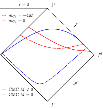
Figure 1: Conformal Carter-Penrose diagram of the Schwarzschild (SS) spacetime depicting four different slices in the outer spacetime. In blue, constant-mean-curvature (CMC) slices, where the trace of the extrinsic curvature ($K=-\nabla_{a}n^{a}$, with $n^{a}$ the future-pointing unit normal vector to the slice) takes the constant value of $-1$. The expression for the height function used is (20) in [49] with $A(\tilde{r})=1=2M/\tilde{r}$. In red, slices determined by the height function (50). The dashed lines employ height functions that correctly take into account the value of the Schwarzschild black hole’s mass, starting from Kerr-Schild coordinates and setting $m_{C_{+}}=-4M$, while the solid lines do not include the effect of the mass ($m_{C_{+}}=0$) – and thus reach $i^{0}$ instead of future null infinity.

With this construction, the Jacobians to change from $(T,R)$ to $(t,r)$ derivatives are given by

$$\partial_{R}=\frac{1}{R^{\prime}(r)}\partial_{r}+\left(1-\frac{1}{R^{\prime}(r)}-\frac{m_{C_{+}}}{R(r)}\right)\partial_{t}\,,$$

$$\partial_{T}=\partial_{t}\,,$$ (51)

where we see that the mass-term places a correction that dominates the term coming from the compactification itself.

The eikonal approach:

Our second approach to construct a hyperboloidal time coordinate is by defining

$$t=u+r$$ (52)

where $u$ satisfies the eikonal equation

$$\nabla^{c}u\nabla_{c}u=0\,.$$ (53)

As explained in [35], demanding that $\nabla^{a}u\propto\xi^{a}$ leads to having outgoing coordinate lightspeeds identically one in the compactified hyperboloidal coordinates. This means that hyperboloidal slices built this way adapt dynamically so that we can control outgoing speeds and should help avoid undesirable coordinate red and blue-shift effects on outgoing signals.

The idea in the eikonal approach is to derive equation (53) and project it along $\underline{\sigma}^{a}$ to get an evolution equation for $U^{-}\equiv\nabla_{\underline{\sigma}}u$, which can then be solved alongside the rEFEs, while the condition $-\nabla^{a}u\propto\sigma^{a}$ gives a fixed functional form to $U^{+}\equiv D_{\sigma}u$ in terms of $U^{-}$ and the metric variables. The equation we get for $U^{-}$ is of advection-type, with principal part decoupled from the principal part of the rEFEs, so symmetric-hyperbolicity of the composite system is trivially preserved.

Similarly to the previous sections, the choice we take for the function $u$ that satisfies the eikonal equation can only be made asymptotically, as parity of $u$ at the origin is complicated and in any case is incompatible with black hole excision. The reason for this is that since the eikonal coordinates forces the outgoing lightspeeds to be identically one, we necessarily need boundary conditions at the black hole boundary. To overcome these obstacles, we place a source $S$ in the right-hand-side of equation (53), instead solving

$$\nabla^{c}u\nabla_{c}u=S\,,$$ (54)

and choosing $S$ so that $u\simeq T-R$ near the origin/horizon and satisfies the eikonal equation identically only near $\mathscr{I}^{+}$. This reduces the Jacobians to the identity when $R$ is small whilst allowing them to take the desired form near $\mathscr{I}^{+}$. (See [35] for full details).

Concretely, if we decompose the vector $u^{a}\equiv-\nabla^{a}u$ with the identity

$$u^{a}=\frac{e^{\delta}}{\kappa}(U^{-}\sigma^{a}+U^{+}\underline{\sigma}^{a})$$ (55)

the evolution equation for $U^{-}$ reads

$$u^{a}D_{a}U^{-}=(u^{a}D_{a}\underline{\sigma}^{b})u_{b}+\tfrac{1}{2}D_{\underline{\sigma}}S\,.$$ (56)

When the expressions on the right-hand-side are expanded out we see that they in fact contain incoming null derivatives of $C_{+}$. Rewriting this equation in the compactified hyperboloidal coordinates requires multiplying by $R^{n}$, so the improved asymptotic decay of $C_{+}$ is needed just as in the height function setting. The sourced eikonal equation (54) places a constraint for $U^{+}$ of the form

$$U^{+}=-\frac{\kappa}{2U^{-}}e^{-\delta}S\,.$$ (57)

The Jacobians in this setting that change from $(T,R)$ derivatives to $(t,r)$ ones are

$$\partial_{R} =\frac{1}{R^{\prime}(r)}\partial_{r}+\left(\frac{e^{\delta}}{\kappa}(U^{+}-U^{-})+\frac{1}{R^{\prime}(r)}\right)\partial_{t}\,,$$

$$\partial_{T} =\frac{e^{\delta}}{\kappa}(C_{+}U^{-}-C_{-}U^{+})\partial_{t}\,.$$ (58)

II.6 Bondi Mass

In the spherical setting, for each hyperboloidal slice, the Bondi mass [50] can be found by taking the limit of the Misner-Sharp mass as one tends to $\mathscr{I}^{+}$. From our expression for $M_{\mathrm{MS}}$, eq. (19), this leads to the expression

$$M_{\text{B}} \equiv\lim_{R\to\infty}M_{\text{MS}}$$

$$=\lim_{R\to\infty}\frac{1}{4}RE^{-}+\frac{1}{8}\big{(}2\tilde{C}^{-}-2\tilde{C}_{+}+4\Delta-2E^{+}$$

$$\quad+(\tilde{C}_{+}+\tilde{C}_{-})E^{-}+E^{-}E^{+}-4E+3E^{-}E\big{)}$$ (59)

Recalling that $\epsilon$ has improved asymptotic decay, the first term is formally singular, meaning it attains a finite limit by a product of a term that diverges, $R$, and a term that decays at least as $O(R^{-1})$, namely $E^{-}$. As opposed to previous formally singular terms appearing in the equations of motion, the evaluation of this term by use of L’Hôpital’s rule is cumbersome. However, since at the continuum level all physical quantities are defined up to constraint addition, and noting that precisely this reduction variable appears in the $\underline{\sigma}^{a}$ component of the GHG constraints (eq. (28)), the expression for $M_{\text{B}}$ can be regularized by a constraint addition that asymptotes at leading order to $-R^{2}C^{\underline{\sigma}}/4$. With this particular choice the regularized expression for $M_{\text{B}}$ reads instead

$$M_{\text{B}}=\frac{1}{4}\left(-\tilde{C}_{+}-\tilde{C}_{-}+F_{D}-E^{+}-2\Theta^{-}\right)$$ (60)

where clearly all terms are now regular $O(1)$ at $\mathscr{I}^{+}$. It is this expression that will be used when we evaluate $M_{\text{B}}$ for our numerical simulations.

The Bondi mass has to satisfy two requirements for a physical solution of the EFEs. First it has to be non-negative, and second it should be monotonically decreasing as radiation leaves the spacetime through $\mathscr{I}^{+}$. This last property can be deduced at the continuum level by the Bondi mass-loss formula, which in terms of our matter model, variables, our particular constraint addition and choice of gauge reads

$$\dot{M}_{\text{B}}=-\pi(\Psi^{-})^{2}\,.$$ (61)

II.7 Constraint Satisfying Initial Data

The evolution Eqs. (26) are equivalent to the EFEs only when the GHG constraints are identically satisfied over the entire domain. As these constraints satisfy a system of coupled second-order nonlinear homogeneous hyperbolic PDEs [51, 52], they remain satisfied throughout the evolution if they are satisfied in the initial data up to their first time derivative. To obtain this formal evolution system satisfied by the harmonic constraints we just have to take a divergence of the rEFEs (26). Being a free evolution scheme, the GHG formulation of the EFEs provides us with no other way to ensure that these constraints are satisfied throughout the evolution.

Recall that we employ two sets of coordinates, namely $X^{\underline{\alpha}}$, which are used to define the tensor basis for the GHG formulation, and the compactified hyperboloidal coordinates $x^{\alpha}$. To avoid confusion in our discussion of the constraints it is therefore most convenient to rely on the rEFEs in abstract index form as in (26). Trace-reversing the rEFEs and contracting once with $n^{a}$, the future pointing unit normal to our hyperboloidal (constant $t$) slices gives

$$\nabla_{n}C_{a} =2\mathcal{M}_{a}+(n_{a}\gamma^{bc}-n^{c}\gamma_{a}{}^{b})\nabla_{b}C_{c}$$

$$\quad+2W_{ab}n^{b}-n_{a}W\,,$$ (62)

with $\mathcal{M}_{a}=(G_{ab}-8\pi T_{ab})n^{b}$ similar to the expression given in [52], $W$ the trace of the constraint addition tensor $W_{ab}$ and $\gamma_{ab}$ the spatial metric. Here $C_{a}$ is the one form of the GHG constraints defined in the $X^{\underline{\alpha}}$ tensor basis by (24), and $\mathcal{M}_{a}=0$ encodes the Hamiltonian and momentum constraints associated with the hyperboloidal foliation. From this expression we observe that it is sufficient to choose initial data that satisfy the harmonic constraints together with data that satisfy the standard Hamiltonian and momentum constraints as usual. From this we then need to reconstruct the evolution variables employed in our formulation.

Given the spatial metric and extrinsic curvature associated with $t$ in the initial data, a general strategy for the latter step can be formulated within the language of [34]. In broad strokes, this would involve constructing appropriate projections of the Jacobians that map between the two coordinate tensor bases, choosing the lapse function of the uppercase $T$ foliation, together with its Lie-derivative along the uppercase normal vector to the $T$-foliation, and then combining these quantities to build the uppercase spatial metric and extrinsic curvature. From there we could choose the uppercase shift vector and switch to our desired choice for the evolved variables. This warrants a careful treatment without symmetry, but for now we settle on a bespoke spherical approach sufficient for our present needs.

We begin with a collection of useful expressions. First we express the spatial metric and extrinsic curvature associated with the time coordinate $t$ in terms of our variables. To accomplish this, we treat $t$ as a general time coordinate that defines a foliation and $r$ to be a radial coordinate on those slices. Later, we shall take the special case of hyperboloidal coordinates. The uppercase coordinates $(T,R)$ are then taken as

$$T\equiv T(t,r)\,,\quad R\equiv R(r)\,.$$ (63)

The metric in the lowercase coordinates can then be defined in terms of the Jacobians $J_{\mu}{}^{\underline{\mu}}\equiv\partial_{\mu}X^{\underline{\mu}}$ as

$$g_{\mu\nu}=J_{\mu}{}^{\underline{\mu}}J_{\nu}{}^{\underline{\nu}}\,g_{\underline{\mu\nu}}\,,$$ (64)

with $g_{\underline{\mu\nu}}$ given in (9). Denoting $t$ and $r$ derivatives by dot ($\dot{}$) and prime (^′), respectively, and the future directed unit normal to the constant $t$ hypersurfaces by $n^{a}$, the standard ADM variables lapse, shift and spatial metric, denoted in the standard notation, are expressed in terms of the GHG ones as,

$$\alpha=\frac{e^{\delta/2}\,R^{\prime}\,\dot{T}\,\sqrt{\kappa}}{\sqrt{2}\,\sqrt{R^{\prime}-C_{-}T^{\prime}}\,\sqrt{R^{\prime}-C_{+}T^{\prime}}}\,,$$

$$\beta^{r}=-\frac{\dot{T}\left((C_{+}+C_{-})\,R^{\prime}-2C_{+}C_{-}T^{\prime}\right)}{2\,(R^{\prime}-C_{-}T^{\prime})\,(R^{\prime}-C_{+}T^{\prime})}\,,$$

$$\gamma_{ij}=\left(\begin{array}[]{ccc}\gamma_{rr}&0&0\\ 0&R^{2}\,e^{\epsilon}&0\\ 0&0&R^{2}\,e^{\epsilon}\sin^{2}\theta\\ \end{array}\right)\,,$$ (68)

with

$$\gamma_{rr}=\frac{1}{\gamma^{rr}}=\frac{2e^{\delta}}{\kappa}\left(R^{\prime}-C_{-}T^{\prime}\right)\left(R^{\prime}-C_{+}T^{\prime}\right)\,.$$ (69)

Similarly, the extrinsic curvature, given by $K_{ij}=-{\cal L}_{n}\gamma_{ij}/2$, takes the form

$$K_{ij}=\left(\begin{array}[]{ccc}K_{rr}&0&0\\ 0&K_{\theta\theta}&0\\ 0&0&K_{\theta\theta}\,\sin^{2}\theta\\ \end{array}\right)\,,$$ (73)

with

$$K_{rr}\equiv\frac{\beta^{r}\,\gamma_{rr}^{\prime}+2\,(\beta^{r})^{\prime}\,\gamma_{rr}-\dot{\gamma}_{rr}}{2\alpha}\,,$$

$$K_{\theta\theta}\equiv\frac{R^{2}\,e^{\epsilon}}{\alpha}\left(\frac{R^{\prime}\,\beta^{r}}{R}+\frac{\left(\beta^{r}\,\epsilon^{\prime}-\dot{\epsilon}\right)}{2}\right)\,.$$ (74)

Plugging (69) into the former of these expressions results in an evolution equation involving our variables. We also define the normal and radial derivatives for the massless scalar field $\psi$ described above as

$$\psi_{n}\equiv{\cal L}_{n}\psi=n^{\mu}\partial_{\mu}\psi\,,\quad\psi_{r}\equiv\partial_{r}\psi\,,$$ (75)

and the corresponding charge and current densities by

$$\rho_{\psi}=\frac{1}{2}\left(\psi_{n}^{2}+\gamma^{rr}\,\psi_{r}^{2}\right)\,,\quad j^{r}_{\psi}=\gamma^{rr}\,\psi_{n}\,\psi_{r}\,.$$ (76)

The nontrivial components of the vector $\mathcal{M}_{a}$ are then

$$\mathcal{H}\equiv 2\,\mathcal{M}_{n}\equiv 2n^{a}n^{b}\left(R_{ab}-\frac{1}{2}g_{ab}R-8\pi T_{ab}\right)\,,$$ (77)

and

$$\mathcal{M}_{r} \equiv n^{a}\gamma_{r}{}^{b}\left(R_{ab}-\frac{1}{2}g_{ab}R-8\pi T_{ab}\right)\,.$$ (78)

In terms of the above variables, and ${}^{\gamma}K_{rr}\equiv K_{rr}\gamma^{rr}$ and ${}^{\gamma}K_{T}\equiv K_{\theta\theta}\gamma^{\theta\theta}$, the Hamiltonian and momentum constraint equations are expressed as

$$2\,{}^{\gamma}K_{T}^{2}+4\,{}^{\gamma}K_{rr}\,{}^{\gamma}K_{T}-16\pi\rho-\frac{2\left(R^{\prime}\,(\gamma^{rr})^{\prime}+2\,R^{\prime\prime}\,\gamma^{rr}\right)}{R}$$

$$+\frac{2(e^{-\epsilon}-R^{\prime 2}\,\gamma^{rr})}{R^{2}}-\left((\gamma^{rr})^{\prime}+\frac{6\,R^{\prime}\,\gamma^{rr}}{R}\right)\epsilon^{\prime}-\frac{3}{2}\gamma^{rr}\,\epsilon^{\prime 2}$$

$$-2\,\gamma^{rr}\,\epsilon^{\prime\prime}=0\,,$$ (79)

and

$$-8\pi\,j_{r}+\frac{2\,R^{\prime}}{R}({}^{\gamma}K_{T}-{}^{\gamma}K_{rr})+({}^{\gamma}K_{T}-{}^{\gamma}K_{rr})\,\epsilon^{\prime}$$

$$+2\,{}^{\gamma}K_{T}^{\prime}=0\,,$$ (80)

respectively. Along with the GHG constraints these are the equations that need to be satisfied by initial data to ensure we obtain solutions of GR. Our bespoke procedure for spherical initial data is divided into three steps:

• Reformulate the Hamiltonian and momentum constraints, eqs. (79) and (II.7). Here, we work assuming that the initial matter distribution $\psi_{n}$ and $\psi_{r}$ and the Jacobian are given.

• Formulate the GHG constraints (28). At this stage one can choose initial data for the gauge driver $f_{D}$ defined in (37).

• Make a concrete choice for the foliation and solve the constraints. Here, we can specify $T(t,r)$ at $t=0$ to construct the initial slice of interest, which is hyperboloidal in our case. This way, we keep the entire procedure general and keep the first two steps agnostic to the choice of foliation.

We see that both Hamiltonian and momentum constraint equations are formally singular at the origin and at $\mathscr{I}^{+}$. To regularize these equations, we extensively use the fact that spherically symmetric vacuum solutions, like Minkowski and Schwarzschild, are the solutions to these equations. To facilitate this, we shall take the general solution to a nontrivial matter distribution to be corrections over these vacuum solutions. This idea has been extensively explored in a series of works about formulations of the constraint equations [53, 54, 55, 56, 57, 58, 59] with different PDE character.

The GHG constraint equations are much easier to solve due the fact that they contain time derivatives of our evolved fields $C_{\pm}$ and which can simply be set. Trivial data for $f_{D}$ leads to undesired asymptotics for $\dot{C}_{-}$. Nonetheless, the latter can be fully controlled by carefully choosing $f_{D}$ in the initial data, which we shall do while solving for the GHG constraints.

A significant advantage of this approach is that all these results apply to any spacetime foliation. For our specific interests, we shall restrict ourselves to the hyperboloidal foliations constructed via the height function and eikonal approach described above, and study the nonlinear perturbations of Minkowski and Schwarzschild backgrounds.

II.7.1 Minkowski perturbations

For the Minkowski spacetime in global inertial time and standard spherical polar coordinates, $C_{+}=-C_{-}=1$ and $\delta=\epsilon=0$, all with vanishing time derivatives. This gives a simplified form to the ADM variables defined in Eqs. (68)-(74), that we shall denote with the subscript “MK”, for Minkowski, for example $\alpha_{\text{MK}}$. We will utilize these values to simplify the general constraint equations.

As mentioned above, our first step is to solve the Hamiltonian and momentum constraint equations. We choose to solve them for $\gamma^{rr}$ and ${}^{\gamma}K_{T}$, respectively, as these equations are linear in these variables. Assigning the Minkowski values obtained above to ${}^{\gamma}K_{rr}$ and $\epsilon$, and taking the substitution

$${}^{\gamma}K_{T}={}^{\gamma}K^{\text{MK}}_{T}+\frac{K_{T}^{(1)}}{R}\,,\quad j^{r}=j^{r}_{\psi}\,,$$ (81)

reduces the momentum constraint equation to

$$(K_{T}^{(1)})^{\prime}=4\pi\,R\,\psi_{n}\,\psi_{r}\,.$$ (82)

To set ${}^{\gamma}K^{\text{MK}}_{rr}$ and ${}^{\gamma}K^{\text{MK}}_{T}$ and so forth, we choose the Minkowski values for our evolved variables just stated, then apply the Jacobian transformations given above. This equation is regular whenever $\psi_{n}\,\psi_{r}\sim 1/R$ in the initial data. Thereby, the entire impact of the current $j_{r}$ is now contained in the correction term $K_{T}^{(1)}$. Setting moreover $\psi_{n}=0$ and imposing the boundary condition $K_{T}^{(1)}=0$ at the origin, we obtain the trivial solution for $K_{T}^{(1)}$ in the initial data. Further, taking

$$\gamma^{rr}=(\gamma_{\text{MK}})^{rr}+\frac{\gamma^{(1)}}{R^{\prime 2}\,R}\,,\quad\rho=\rho_{\psi}\,,$$ (83)

gives the simple form

$$(\gamma^{(1)})^{\prime} =\,-4\pi R^{2}R^{\prime}\,\psi_{r}^{2}\left((\gamma_{\text{MK}})^{rr}+\frac{\gamma^{(1)}}{RR^{\prime}}\right)\,,$$ (84)

to the Hamiltonian constraint equation, which is regular whenever $\psi_{r}\sim 1/R$ in the initial data. For this class of initial data, all information of the initial matter distribution $\psi_{r}$ is now encoded in $\gamma^{(1)}$. This is the final equation we solve for generating the Hamiltonian and momentum constraint satisfying initial data in the Minkowski case.

The second step involves solving the GHG constraints (28). We will solve them for $\dot{C}_{+}$ and $\dot{C}_{-}$ using the gauge source functions given in (37), along with all the simplifying assumptions and solutions to the Hamiltonian and momentum constraint equations given above. We further take $p=0$ in the gauge source functions and $C_{+}=-C_{-}=1$ in the initial data, which translates to the ADM variables as

$$\alpha=\left(\alpha_{\text{MK}}\,\sqrt{\gamma_{rr}\,(\gamma_{\text{MK}})^{rr}}\right)\,,\quad\beta^{\mu}=\beta^{\mu}_{MK}\,.$$ (85)

Now we observe that the trivial data for the gauge driver $f_{D}$ gives data for $\dot{C}_{-}$ which is nonzero and $O(1)$ at $\mathscr{I}^{+}$. This inconsistency contradicts our regularization scheme adopted from [40, 41, 42]. As previously noted, the data for $f_{D}$ is sufficient to establish the asymptotic behavior of $\dot{C}_{-}$ in the initial data to any desired level. For our convenience, we opt for a choice that causes it to decay more rapidly than any inverse power of $R$. One such choice is

$$f_{D}=- \Bigg{(}\frac{\gamma^{(1)}}{R^{\prime 2}R}-\frac{\beta_{\text{MK}}^{r}}{\dot{T}R^{\prime}}\left(1-\sqrt{1+\frac{(\gamma_{\text{MK}})_{rr}\,\gamma^{(1)}}{RR^{\prime 2}}}\right)\Bigg{)}\times$$

$$\frac{2\chi(R)R^{\prime}\left(R^{\prime}+T^{\prime}\right)}{R}\,,$$ (86)

and $\dot{F}_{D}=0$. Interestingly, this data depends on the foliation. This exhausts all our requirements to build the data. To sum up, we have assigned Minkowski values to $C_{\pm}$, $\epsilon$ and ${}^{\gamma}K_{rr}$, which translates to $\dot{\delta}$. The Minkowski values are determined by transforming the global inertial values of our evolved variables through the appropriate Jacobians. We must then solve the constraints to obtain $\dot{C}_{\pm}$, $\gamma^{rr}$ and ${}^{\gamma}K_{T}$. The last two translate to $\delta$ and $\dot{\epsilon}$ in the data. We have also established data for the matter and the gauge driver while ensuring that the asymptotic properties of the ADM variables are satisfied.

The final step is choosing the Jacobians. We consider both the height function and eikonal approaches to define the foliation $T(t,r)$ and keep the same compactification $R(r)$ defined above in both cases. For Minkowski perturbations, we set $m_{C_{+}}=0$ in the height function (50). In our numerical implementation we simply integrate out the resulting ODEs.

The Misner-Sharp mass corresponding to this class of initial data is

$$M_{\text{MS}}^{\text{MK}}=-\frac{1}{2}\gamma^{(1)}\,.$$ (87)

Interestingly, this expression for the mass and the rescalings in the correction terms in (81) and (83) are independent of the foliation. As we conclude from Eq. (84), and observe in Figure 2, $M_{\text{MS}}$ remains positive semi-definite everywhere and $O(1)$ whenever $\psi_{r}$ falls-off at least like $1/R$ towards $\mathscr{I}^{+}$. We will consider the more general case with $\psi_{n}\neq 0$ in the future.

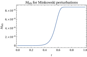
Figure 2: Misner-Sharp mass of Minkowski perturbation initial data with $\psi_{n}=0$ and $\psi=e^{-R(r)^{2}}/10^{3}$ on a hyperboloidal slice constructed via the height function with compactification index $n=1.5$. This initial data gives very similar profile for $M_{\text{MS}}$ as that shown in Figure 8.5 of [31], although the specific amplitude chosen in this plot results in a far smaller Bondi-mass.

II.7.2 Schwarzschild perturbations

Our procedure for perturbed black hole initial data is very similar. The Schwarzschild metric in Kerr-Schild coordinates is given by

$$(g_{\text{SS}})_{\mu\nu}=\left(\begin{array}[]{cccc}-1+\frac{2M}{R}&\frac{2M}{R}&0&0\\ \frac{2M}{R}&1+\frac{2M}{R}&0&0\\ 0&0&R^{2}&0\\ 0&0&0&R^{2}\sin^{2}\theta\\ \end{array}\right)\,.$$ (92)

Here, $M$ represents the mass of the black hole and the subscript “SS” stands for Schwarzschild. Comparing this with the metric in (9), we observe that for the Schwarzschild metric in Kerr-Schild coordinates, we have

$$C_{+}=\frac{1-2M/R}{1+2M/R}\,,\quad C_{-}=-1\,,\quad\delta=\epsilon=0\,,$$ (93)

all with vanishing time derivatives. This gives the associated ADM variables that we denote by the subscript “SS”.

Like before, we set the Schwarzschild values for ${}^{\gamma}K_{rr}$ and $\epsilon$ in the initial data and take

$${}^{\gamma}K_{T}={}^{\gamma}K^{\text{SS}}_{T}+\frac{(K_{\text{SS}})_{T}^{(1)}}{R}$$ (94)

to get the momentum constraint equation similar to (82). Once again, we set $\psi_{n}=0$ to get the trivial solution $(K_{\text{SS}})_{T}^{(1)}=0$ in the initial data. Likewise, taking

$$\gamma^{rr}=(\gamma_{\text{SS}})^{rr}+\frac{(\gamma_{\text{SS}})^{(1)}}{R^{\prime 2}\,R}\,,$$ (95)

gives an equation for $(\gamma_{\text{SS}})^{(1)}$ similar to (84). This equation is regular, as before, with a solution that is regular throughout the domain. Thus we again embed all information of the initial matter distribution in $(\gamma_{\text{SS}})^{(1)}$ and solve it to generate the Hamiltonian and momentum constraints satisfying initial data.

We again take the simplifying conditions

$$\alpha=\left(\alpha_{\text{SS}}\,\sqrt{\gamma_{rr}\,(\gamma_{\text{SS}})^{rr}}\right)\,,\quad\beta^{\mu}=\beta^{\mu}_{\text{SS}}\,,$$ (96)

to get the Schwarzschild values for $C_{\pm}$ and solve the GHG constraints for $\dot{C}_{\pm}$ with the gauge source functions

$$F^{\sigma}_{\text{SS}}=F^{\sigma}+\frac{C_{+}-1}{\mathring{R}}\,,$$ (97)

and $F^{\underline{\sigma}}$ given in (37) with $p=0$. We, additionally, take the following initial data for the gauge driver

$$F^{\text{SS}}_{D}= -\Bigg{(}\frac{\gamma^{(1)}}{R^{\prime 2}R}-\frac{\beta_{\text{SS}}^{r}}{\dot{T}R^{\prime}}\left(1-\sqrt{1+\frac{(\gamma_{\text{SS}})_{rr}\,(\gamma_{SS})^{(1)}}{RR^{\prime 2}}}\right)\Bigg{)}\times$$

$$\quad 2R^{\prime}\left(R^{\prime}+T^{\prime}\right)\,,$$ (98)

and $\dot{f}_{D}=0$ to correct the asymptotics of $\dot{C}_{-}$. This specific choice of $f_{D}$ gives trivial data for $\dot{C}_{-}$ and, interestingly, reduces to (86) for vanishing $M$ and $\chi(R)=R$. This exhausts all our requirements to generate the initial data.

As before, we consider both constructions of hyperboloidal foliation defined above. We take $m_{C_{+}}=-4M$ in the height function.

The Misner-Sharp mass in this case is given by,

$$M_{\text{MS}}^{\text{SS}}=M-\frac{1}{2}(\gamma_{\text{SS}})^{(1)}\,,$$ (99)

with $(\gamma_{\text{SS}})^{(1)}$ having similar properties as in the Minkowski case, and effectively increasing the mass of the initial data.

III Numerical Evolutions

Our numerical implementation lies within the infrastructure used in earlier works, the most similar systems being [30, 43, 44, 45]. The method itself is entirely standard, so we give just a brief overview. Evolution is made under the method of lines with fourth order Runge-Kutta. We use second order finite differences in space. Our first order reduction makes the treatment of the origin quite subtle. Following our earlier work we have adapted Evans method [60] (see also [61] for variations) in the obvious manner for the metric components (and their reduction variables) as well as the scalar field. We define in particular two second order accurate finite differencing operators as acting on some given grid-function $f$,

$$D_{0}f =\frac{1}{h}\frac{f_{i+1}-f_{i-1}}{2}\,,$$

$$\tilde{D}f =\frac{1}{h}(p+1)\frac{r^{p}_{i+1}f_{i+1}-r^{p}_{i-1}f_{i-1}}{r^{p+1}_{i+1}-r^{p+1}_{i-1}}\,,$$ (100)

with $h$ the grid-spacing. The parameter $p$ here is not directly related to those that appeared in (37) and (44)). Since we are focused in this work on proof-of-principle numerics, we have not tried to extend the code beyond second order accuracy. This remains an important task for the future, but there is no particular reason to expect difficulties in doing so. Terms in the evolution equations like $\partial_{r}\psi+\tfrac{p}{r}\psi$ are treated with $\tilde{D}$, whereas plain derivatives are approximated by $D_{0}$. As mentioned above, ghostzones to the left of the origin are populated by parity. With this said, the EFEs still contain formally singular terms at the origin. These are managed by application of L’Hôpital’s rule. At $\mathscr{I}^{+}$ we do not require continuum boundary conditions, and so it is permissible simply to shift the finite differencing stencils to the left. To minimize reflections from the outer boundary we use truncation error matching,

$$(Df)_{N}=\frac{1}{4h}(f_{N-4}-5f_{N-3}+10f_{N-2}-11f_{N-1}+5f_{N})\,.$$ (101)

The idea is that by matching the form of the finite differencing error at the boundary with that of the interior, high frequency errors are reduced. Formally singular terms at $\mathscr{I}^{+}$, which appear in our first order reduction in exactly the same shape as those of the GBUF model we studied earlier [45], are likewise treated with L’Hôpital’s rule. As is standard when using the GHG formulation, we use excision to treat the black hole, should there be one. The strategy is to keep the apparent horizon, the position where the expansion of outgoing null-geodesics vanishes, within the computational domain with the boundary itself remaining outflow, so that no boundary continuum conditions are needed. Due to the relatively simple dynamics in the strong-field region in our experiments, this can be done without the full control system machinery [62] used in binary spacetimes, and without any careful imposition of the outflow condition [63]. Instead we simply monitor the position of the apparent horizon, which is very simple in spherical symmetry (see [64] for a textbook discussion), and monitor the coordinate lightspeeds at the boundary to check that the outflow condition is satisfied. Typically we take the domain to extend a small number of points inside the apparent horizon. To compute derivatives at the excision boundary we populate ghostzones by fourth order extrapolation. When evolving initial data that collapse to form a black hole we must use our two finite differencing operators. If instead we start from data that already contains a black hole we can do away with the $\tilde{D}$ operator. We have implemented both possibilities. We study numerical evolution of various different choices of initial data. They are described in turn in the following subsections.

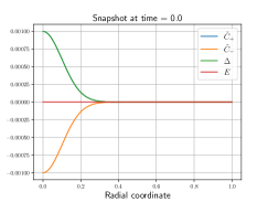
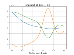
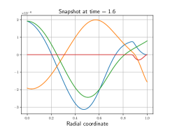
Figure 3: In these plots we show snapshots of the evolved variables $\tilde{C}_{\pm},\epsilon$ and $\delta$ from an evolution with height function Jacobians with $n=1.5$, and a pure gauge perturbation for the initial data. Note that the initial data in the region $(r_{m},1)$ is sufficiently small so that most of the perturbation lies in the region where Cauchy and hyperboloidal slices match. Observe that as expected the fields $\tilde{C}_{+}$ and $E$ vanish at $\mathscr{I}^{+}$ ($r=1$ in our coordinates) at all times whereas $\tilde{C}_{-}$ and $\Delta$ oscillate. At later times the remnant features continue to shrink.

III.1 Gauge Perturbations

As a first test we perform numerical evolutions of gauge perturbations of Minkowski spacetime. The simplest procedure to input this type of initial data is to construct our slices with hyperboloidal layers, as explained in [13], so the nontrivial field content lies inside the region where the change of coordinates, in this case from Minkowski in global inertial time and spherical polars, to compactified hyperboloidal coordinates, is simply the identity. Concretely, we use the same expression (50) for the height function with $m_{C_{+}}=0$ and we take $r_{m}=0.4$. In the $3+1$ language we place a Gaussian perturbation in the lapse with amplitude $A$ and zero shift. In terms of our variables this corresponds to

$$C_{+}(0,r)=1+Ae^{-R(r)^{2}/\sigma_{0}^{2}}\,,$$

$$C_{-}(0,r)=-1-Ae^{-R(r)^{2}/\sigma_{0}^{2}}\,,$$

$$\delta(0,r)=\ln(1+Ae^{-R(r)^{2}/\sigma_{0}^{2}})\,,\quad\epsilon(0,r)=0\,,$$

$$\psi(0,r)=0\,,\quad f_{D}(0,r)=\partial_{T}f_{D}(0,r)=0\,.$$ (102)

where we take $\sigma_{0}^{2}=0.02$.

The form of the perturbation differs from that in [30] only in that the present perturbation is centered at the origin. Observe that the choice of GHG implies an evolution equation for the lapse and shift. In our variables this corresponds to a non-zero time derivative of the shift which is equivalent to

$$\partial_{T}C_{+}(0,r)=-2A\frac{e^{-2R^{2}/\sigma_{0}^{2}}}{\sigma_{0}^{2}}\left(A+e^{R^{2}/\sigma_{0}^{2}}\right)R\,,$$

$$\partial_{T}C_{-}(0,r)=-2A\frac{e^{-2R^{2}/\sigma_{0}^{2}}}{\sigma_{0}^{2}}\left(A+e^{R^{2}/\sigma_{0}^{2}}\right)R\,,$$

$$\partial_{T}\delta(0,r)=0\,,\quad\partial_{T}\epsilon(0,r)=0\,.$$ (103)

With these expressions we construct the FOR fields to perform the numerical evolutions. By construction, this initial data satisfies the constraints up to numerical error.

Evolving the data, the dynamics look similar in both the height function and eikonal setup. The gauge pulses initially propagate outwards and through $\mathscr{I}^{+}$ with no sign of reflection. They leave behind small perturbations in the evolved fields which later gradually decay. We chose to work with the gauge parameters $p=0$ in (37), meaning that the variables $C_{+}$ and $\epsilon$ should have improved asymptotic decay relative to the wave equation, whilst $C_{-}$ and $\delta$ should behave like solutions to the wave equation. Since the scalar field vanishes identically in this case, the gauge driver field $f_{D}$, which we feed trivial initial data, does too. Even at moderate resolution the method successfully runs for long-times, at least until $t=10^{4}$ in code units. The differences in asymptotics of the variables is well captured by the numerical evolution, and the harmonic constraints remain small throughout. Evolving for instance with $200$ radial grid-points, at $t=10$ the harmonic constraints are of order $O(10^{-8})$. In Figure 3 we present snapshots of the evolved fields for an evolution with eikonal Jacobians with compactification parameter $n=1.5$ at this resolution. These evolutions exhibit both pointwise and norm convergence. To demonstrate this, in Figure 4 we plot snapshots of rescaled differences at three resolutions for the same setup as in the snapshots of Figure 3. To avoid overpopulating the figure we have taken the sum of absolute value of these differences over all four of the fields plotted in the first figure. The data are perfectly compatible with second order convergence as desired. These results are in excellent qualitative agreement with those of [30], with a different formulation of GR.

Interestingly, not all compactification parameters $n$ behave in the same manner numerically at the moderate resolution we employ. Despite the continuum freedom to choose it at the analytical level, only for values $n\leq 1.5$ we get the appropriate norm-convergence with increasing resolution. This can be understood from the empirical observation that for bigger values the reduction fields get sharp features at the grid-point at $\mathscr{I}^{+}$, therefore affecting the precise numerical cancellation that needs to happen in order for this scheme to work. We believe that by adjusting the compactification we will be able to achieve convergent results for the entire range of $n$, but since this fact is seen in all of our subsequent numerical evolutions, in practice we work in the range $n\in[1.25,1.5]$ here.

Pure gauge wave evolutions on the Schwarzschild background behave similarly, but since physical dynamics, which we discuss thoroughly below, necessarily excite gauge waves we do not present them in detail here.

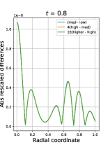
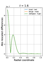
Figure 4: Here we show pointwise convergence of our method in the gauge wave configuration of Figure 3. Specifically we performed three numerical evolutions, doubling resolution twice. We then take the differences of the solutions and rescale according to second order convergence. We then take the absolute value of these differences and sum over the variables presented in Figure 3. Coincidence of the two curves is thus compatible with second order convergence.

III.2 Constraint Violating Initial Data

We now move on to our hardest set of numerical tests, which comprise of constraint violating initial data with non-vanishing scalar field. It is important to consider constraint violating data because in general numerical error violates the constraints in any free-evolution setup, and so we must be confident that at least reasonably small finite errors of this type will not cause a catastrophic failure of the method. Since these initial data excite also gauge pulses, all aspects of the solution space including gauge, constraint violations and physical are probed. In all of the following tests we see similar results for height function and eikonal Jacobian, so we present a selection of representative plots from each.

Minkowski perturbations:

In the following we performed tests both with and without layers, with $r_{m}=0.4$ and $r_{m}=0$. Both behave similarly, so we present results only for the case $r_{m}=0$. We begin by perturbing the Minkowski metric, setting Gaussian data on all variables according to

$$C_{+}(0,r)=1+C_{0}e^{-R(r)^{2}}\,,\quad C_{-}(0,r)=-1-C_{0}e^{-R(r)^{2}}\,,$$

$$\delta(0,r)=\delta_{0}e^{-R(r)^{2}}\,,\quad\epsilon(0,r)=(\delta_{0}-\ln(1+C_{0}))e^{-R(r)^{2}}\,,$$

$$\psi(0,r)=\psi_{0}e^{-R(r)^{2}}\,,\quad f_{D}(0,r)=0\,,$$ (104)

with vanishing time derivatives. The initial data for the rescaled FOR variables are then calculated accordingly. Therefore in this first test the reduction constraints should remain satisfied at the continuum level. When evolving with the eikonal Jacobians we choose data appropriate for the Minkowski spacetime in global inertial coordinates, namely

$$U^{-}=e^{-\delta(0,r)}\left(2+C_{0}e^{-R(r)^{2}}\right)\,,$$ (105)

with the variable $U^{+}$ taken from the sourced eikonal equation itself (57).

The coefficients of the Gaussian in the initial data for $C_{\pm}$ are chosen to give the correct parity at the origin. Similarly, the coefficient of the Gaussian in the data for $\epsilon$ is chosen from the regularity condition (32) at the origin at $T=0$. Unsurprisingly, if we take data that violate parity the code is observed to crash near the origin in finite time.

As a first test we kept the initial perturbations small enough to avoid complete gravitational collapse. For simplicity, we took $C_{0}=\delta_{0}=\psi_{0}=10^{-3}$. This data do not satisfy the GHG, Hamiltonian or Momentum constraints. The magnitude of the GHG constraint violation in the initial data is $10^{-4}$, comparable with the scalar field itself. We performed numerical evolutions with both the height-function and eikonal Jacobians, with several different values of the compactification parameter $n$ within the range specified at the end of the previous subsection. In all cases the time evolution is comparable to the gauge wave discussed above in section III.1. The initial constraint violation initially grows and eventually decays, so that by $t=10$ it has reduced by $1$ order of magnitude. Similar comments apply to the $L^{2}$ norm of the constraints. These data are clearly physically wrong from the outset since the Bondi mass initially vanishes despite the fact that the scalar field is non-trivial, and even takes negative values during the evolution. We observe this behavior both in the original (59) and regularized (60) expressions for the Bondi mass, with the former not even varying monotonically due to constraint violations.

Another important difference between these experiments and the pure gauge waves is that the gauge driver variable $f_{D}$ now actually varies. Recall that the purpose of the gauge driver is to prevent log-terms, which are known to afflict plain harmonic gauge, from appearing in the variable $C_{-}$. Using the gauge driver condition (38) we see no evidence that these log-terms are present. Given the rescaling in the definition of our variables (43) such log-terms would result in divergence of the solution, and so should be very obvious. To check this, we evolved the constraint violating data (104) without using the gauge driver, with identical initial data, and find that the growth in $\tilde{C}_{-}$ is indeed evident, as can be seen in Figure 5. In fact, evolutions without the gauge driver can only be performed in a staggered grid, as having a grid-point at $\mathscr{I}^{+}$ leads to an explosion of the simulation after the first time step. All of our simulations except this were performed with a with a grid-point at future null infinity. Earlier work has been presented with a combination of these two setups. For instance the evolutions of [30] were performed on a staggered grid, whereas in [32] the grid setup was identical to that in the majority of our simulations.

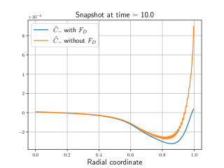
Figure 5: Here we plot the evolved field $\tilde{C}_{-}$ for simulations performed with and without the gauge driver, for identical initial data, with a staggered grid and with $n=1.5$. From the figure it is obvious that the absence of $F_{D}$ makes $\tilde{C}_{-}$ diverge at $\mathscr{I}^{+}$, as expected from the continuum analysis, and explained in more detail in the main text. On the contrary, the presence of $F_{D}$ makes the evolved fields regular there. It is important to mention that both evolutions were performed with the same numerical techniques, thus the divergent behavior does not follow from numerical error.

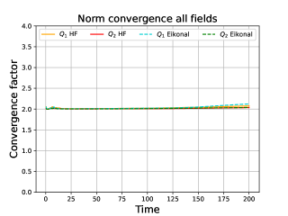
Figure 6: Here we plot the norm self-convergence rate obtained in evolutions of constraint violating data with a regular center, with both height function and eikonal Jacobians and compactification parameter $n=1.4$. The two curves from each case correspond to the rate obtained from three numerical evolutions, $Q_{1}$ the triple including the lowest resolution and $Q_{2}$ the highest. For our discretization we would expect the curves to lie at two. Observe that although there is a drift $Q_{1}$ at late times, this feature is suppressed in $Q_{2}$, meaning that it converges away with resolution. Looking at the raw data we see that this drift is caused by noise in the dissipation operator at $\mathscr{I}^{+}$, which is of third order, and so we see the drift tending to values bigger than two. Details of the initial data and norms are given in the main text.

Next we switched the gauge driver back on. We performed four numerical evolutions, doubling resolution each time, so that we could examine multiple curves. Pointwise convergence of the fields at early times looks very much like that presented in Figure 4. In Figure 6 we plot the norm self-convergence rate from these long experiments. For the test itself we apply the standard technique, injecting the higher resolution data on to the coarse resolution grid, taking the norm of the differences between the very high ($V$) and high ($H$) resolutions, the high and medium ($M$) resolutions, and finally medium and low ($L$) resolutions. We then plot

$$Q_{1} =\log_{2}\left(\frac{||M-L||}{||H-M||}\right)\,,\quad Q_{2}=\log_{2}\left(\frac{||H-M||}{||V-H||}\right)\,,$$ (106)

as a function of time, from which it can be seen that the simulations converge at second order as we increase resolution, as expected with our discretization. Concretely, given a field $Z(t,r)$ and its two associated first order reduction fields $Z^{+}\,,Z^{-}$, see the discussion around (41), the continuum limit of the norm we use is,

$$\int\left[r^{2}Z^{2}+\left(\frac{R^{\prime}R^{2}}{\chi^{2}}\right)\left(\frac{2R^{\prime}-1}{2R\textasciiacute\chi^{2}}(Z^{+})^{2}+\frac{1}{2R^{\prime}}(Z^{-})^{2}\right)\right]dr\,.$$ (107)

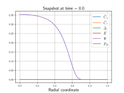
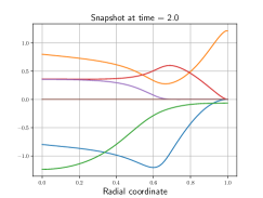
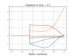
Figure 7: Here we show snapshots of the evolved variables in an evolution of constraint violating data large enough to collapse to form a black hole. These evolutions were performed with the height-function Jacobian and with compactification parameter $n=1.5$. Observe that even in this very dynamical scenario the method respects well the expected asymptotic behavior at $\mathscr{I}^{+}$, with certain fields continuing to display improved fall-off. After an apparent horizon forms we evolve using black hole excision as described in the main text. For visual clarity we set the variables to vanish inside the apparent horizon.

No attempt has been made to tune to the threshold of collapse, but increasing the amplitude of the data to $\psi_{0}=0.355$ leads to apparent horizon formation. As explained above, we also implemented excision, so that once an apparent horizon is formed, the black hole interior can be taken out of the evolved region. As a visualization technique, we put all the evolved variables to zero inside the excised region so that we can identify where the apparent horizon was found. Examples of this are shown in Figure 7. Performing longer evolutions we see that the data appear to settle down, although slow dynamics continue. At time $t=50$ substantial constraint violation remains, and pointwise is in fact substantially larger than the scalar field and its reduction variables.

Schwarzschild perturbations:

Next we take initial data of a similar type to (104), but now built as a perturbation on top of the Schwarzschild spacetime. To do so we adjust several details in our evolution setup, focusing henceforth exclusively on the case $r_{m}=0$.

In order to do excision as previously described, we need to start from horizon penetrating coordinates. We take the Schwarzschild solution in Kerr-Schild form, which we recall was given above in our variables in Eq. (93).

Since this is an exact solution of the EFEs, it is desirable to have a choice of gauge for which (93) is static in local coordinates, so that dynamics in the numerical evolution come from the departure from it. To achieve this we adjust the gauge sources (37), in which, as mentioned above (97), the only modification is

$$F^{\sigma}_{\text{SS}}=F^{\sigma}+\frac{C_{+}-1}{\mathring{R}}\,.$$ (108)

It is easy to see that that expressions (93) are an exact solution of the rEFEs with the previous choice of gauge. This fact is reflected numerically in the sense that numerical evolutions with this exact initial data remain unchanged up to numerical error for long times, up to $t\sim 10^{3}M$, even at very modest resolution. Due to the way gauge conditions are constructed, this has not yet been achieved with the approach followed in [49]. We observe that the new term does not alter the asymptotics of the evolved fields, and that we still need the gauge driver $f_{D}$ in order to regularize the $C_{-}$ field in the presence of a scalar field.

For our next numerical test we put constraint violating Gaussian perturbations on top of the solution (93), where we take the BH mass $M=1$ as defining our units here. Analogous to the previous constraint-violating case, the data we start our simulations with is

$$C_{+}(0,r)=\frac{1-\frac{2}{R}}{1-\frac{2}{R}}+C_{p0}e^{-(R-3)^{2}}\,,$$

$$C_{-}(0,r)=-1+C_{m0}e^{-(R-3)^{2}}\,,$$

$$\delta(0,r)=\delta_{0}e^{-(R-3)^{2}}\,,\quad\epsilon(0,r)=\epsilon_{0}e^{-(R-3)^{2}}\,,$$

$$\psi(0,r)=\psi_{0}e^{-(R-3)^{2}}\,,\quad f_{D}(0,r)=0\,,$$

$$U^{-}=e^{-\delta(0,r)}(1-C_{-}(0,r))$$

with the first-order-reduction fields computed assuming vanishing time derivatives. Note that the Gaussians are now centered at $R=3$ and that in this case there is no relation between $\epsilon$ and the amplitude of the other fields, or between $C_{+}$ and $C_{-}$, since we do not have a regular center in this case. We have performed successful evolutions of this data using again both the height-function and eikonal Jacobians with several values of $n$. In broad terms these data develop in a manner similar to the previous setups, in so much that part of the the initial pulses still propagate out to infinity with $O(1)$ speeds. Of course in this case part of the field content also accretes on to the black hole. At infinity the scalar field moreover clearly exhibits the direct signal, ringing and tail phases. These data are particularly important as our first test in which several of the evolved fields have non-trivial ‘mass-terms’ at infinity. We observe no particular difficulty in their numerical treatment, finding both pointwise and norm convergence just as convincingly as in the previous cases with a regular center. As an example of this, in Figure 8 we show the norm self-convergence rates with this setup.

To check the effect of the logarithmic mass term with the height function change of coordinates (50), we performed also tests with that term omitted. We find that the signal tends to accumulate at large $R$ without ever leaving the domain, leading for the evolution to crash in finite time, compatible with our understanding from above in section II.5 that without the mass-term included these slices have the ‘wrong’ global structure, terminating instead at spatial infinity, as depicted in Figure 1. It is clear that the inclusion of the ‘mass-terms’ is a fundamental ingredient in the method.

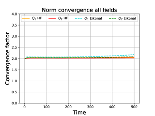
Figure 8: As in Figure 6, here we plot the norm self-convergence rate obtained in evolutions of constraint violating data, but now built as a perturbation of the Schwarzschild spacetime, for both the height function and eikonal Jacobians and with compactification parameter $n=1.4$. Observe that similar drift in the convergence rate at late times occurs as in the regular center case, due to the same reason. This feature converges away with resolution also here, so the method is still satisfactory.

Despite the success in this suite of configurations, we do expect that if we were to take the initial constraint violations, of whatever type, sufficiently large then we could cause our numerical method to fail. We have not attempted to do so, however, since, first, the same statement would be true even in standard Cauchy evolutions and second, the task of the hyperboloidal region is to cope with a combination of stationary features and outgoing waves, with the metric variables decaying out to $\mathscr{I}^{+}$. If we were to face a situation in application in which large errors in the wavezone induced a failure of the method, either more resolution is needed, or else the wavezone, which only loosely defined, ought to be taken to ‘start’ further out and therefore the parameters for the hyperboloidal layer adjusted.

III.3 Constraint Satisfying Initial Data

The rEFEs are a set of wave equations for all the metric variables, so up to this point we have successfully tested our regularization techniques, allowing us to numerically extract the wave signal at $\mathscr{I}^{+}$, the ultimate goal of this project. However, in order to have a physical spacetime that simultaneously solves the EFEs we need to satisfy all the constraints, namely, GHG, Hamiltonian, Momentum and FOR constraints, as explained in section II.7. Therefore, as a final test of our scheme, we move on to evolve constraint satisfying initial data representing perturbations of the Minkowski and Schwarzschild spacetimes.

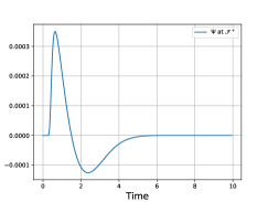
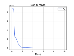
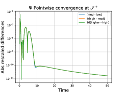
Figure 9: In the left panel of these plots we show the scalar field as a function of time at the grid-point at $\mathscr{I}^{+}$ for the evolution of perturbed Minkowski data. The middle panel displays the evaluation of the Bondi mass for this numerical data, from which we see it satisfies the expected properties for a physically reasonable spacetime. Finally, in the right panel we show the absolute value of the rescaled differences of $\Psi$ at the grid-point at $\mathscr{I}^{+}$ as a function of time for the 4 resolutions used in our simulations. The overlapping of the three curves in this figure show that errors converge away at the expected order with increasing resolution, thus showing that our treatment resolves well the radiation signal asymptotically.

Minkowski perturbations:

We begin by constructing initial data for a spacetime that can be thought as a perturbation of the Minkowski spacetime. We first take the height function approach for constructing the initial hyperboloidal slice, with $m_{C_{+}}\equiv 0$, as demanded by our method explained in section II.7. We choose $\psi(0,r)=\psi_{0}e^{-R^{2}}$ and $\psi_{n}=0$, with $\psi_{0}=10^{-3}$ in order to avoid complete gravitational collapse. With these choices we numerically generate the solution $\gamma^{(1)}$.

A simple way to generate constraint satisfying initial data for hyperboloidal slices built with the eikonal approach is to choose $U^{+}$ and $U^{-}$ initial data so that the Jacobians (II.5) match the height function ones (II.5). Observe that the choice $C_{+}\equiv 1$ automatically implies that the $U^{+}$ constraint, Eq. (57), is satisfied.

With these details taken care of, we evolve the initial data with both the eikonal and height-function equations of motion. The basic dynamics qualitatively resemble those of the constraint violating case, with regular fields both at the origin and $\mathscr{I}^{+}$. For this reason we do not present snapshots in space. Instead, in the first panel of Figure 9 we plot the scalar field waveform at $\mathscr{I}^{+}$, where we clearly see the field decaying at late times.

One of the most stringent test on the physics in the present case is the evaluation of the Bondi mass, Eq. (60) both for the initial data and the time development. As previously mentioned, this should be a non-negative and monotonically decreasing function of time. Both properties can be seen from the middle panel of Figure 9, from which we see that we initially start with a positive constant value until the time radiation leaves the domain through $\mathscr{I}^{+}$. The left and middle panels indeed indicate that the spacetime asymptotes to the Minkowski spacetime as the scalar field leaves the numerical domain.

Within our setup the only physical radiation comes from the scalar field, so our methods can only be claimed successful if this signal is well-captured numerically. As for the constraint violating initial data in section III.2, we performed norm self-convergence test for the constraint satisfying data, obtaining similar results to those shown in Figure 6. Focusing instead on the radiation field, our proxy for gravitational waves, in the third panel of Figure 9, we plot the absolute value of the rescaled differences of the scalar field at the grid-point at $\mathscr{I}^{+}$ as a function of time. The overlapping of the three curves in this case shows that the errors of this radiation signal decrease at the expected rate with increasing resolution, thus implying that in the limit of infinite resolution we tend to the real physical solution.

We proceeded to modify the initial data for the scalar field to $\psi=\psi_{0}e^{-R^{2}/\sigma_{0}^{2}}$, with $\psi_{0}=0.8$ and $\sigma_{0}=0.6$, in order to generate an apparent horizon dynamically, which we see at time $t\sim 0.5$ in code units. Qualitatively, the evolved fields look much like those presented in Figure 7. Interestingly our evolved fields appear somewhat more regular near $\mathscr{I}^{+}$ than those of [31] in the same physical setup. In contrast to the constraint violating collapse, the Bondi mass remains positive and monotonically decreasing for all times settling to a non-zero value for late times. The apparent horizon mass is non-decreasing. After black hole formation the code continues to run without problems for at least $t\sim 10^{3}M$ at moderate resolutions, where $M$ is the Bondi mass at late times.

Schwarzschild perturbations:

In order to generate constraint satisfying initial data for Schwarzschild spacetime perturbations we follow again the steps mentioned in section II.7. We started by generating initial data slice with the height function Jacobians. In the present case we no longer take $m_{C_{+}}=0$. However, in order for the scheme to work we need to know the constant $m_{C_{+}}$ exactly, and therefore we take $C_{+}$ identical to the Schwarzschild solution previously mentioned. We have experimented with various different initial data choices for the scalar field compatible with our present procedure for the constraints.

In order to evolve using eikonal hyperboloidal slices in the present case we again generated initial data for $U^{+}$ and $U^{-}$ so that eikonal Jacobians match initially the height function ones. Importantly, the matching of the Jacobians gives a unique solution for the initial data for $U^{+}$ and $U^{-}$, so the $U^{+}$ constraint (eq. (57)) will not be satisfied for a generic given $S$. To overcome this issue we rather take eq. (57) as defining the function $S$. This choice of $S$ does vanish asymptotically, so with this approach the outgoing radial coordinate lightspeed in lowercase coordinates still goes to unity, which is the desired property when we use the eikonal Jacobians.

The basic dynamics proceed as expected, with part of the scalar field accreting on to the black hole, and the rest gradually propagating out to null infinity. As a specific example, we take a Gaussian profile for the scalar field centered at $R\simeq 2.1M$, with $M=1$ from the reference solution which we perturb, with $\psi(0,r)=\psi_{0}e^{-(R-2.1)^{2}/\sigma^{2}}$, $\sigma=0.2$ and $\psi_{0}=10^{-4}$. The outcome of a long evolution of this data is shown in Figure 10, where we plot the scalar field value at $\mathscr{I}^{+}$ as a function of time for the full non-linear evolutions with the height function Jacobians. From this we see that we recover the expected behavior from linear scalar perturbations on top of Schwarzschild, where we see that the spherically-symmetric quasi-normal mode of $\psi$ is in good agreement with the first part of the data, while late time evolution decays as $t^{-2}$. This is in qualitative agreement with the earlier free-evolution results of [65, 31] under different gauges on a staggered grid (see Figure 3 of [65] and Figure 8.24 in [31]). For comparison we also performed evolutions in the Cowling approximation, which corresponds to taking Schwarzschild spacetime as the fixed background and evolving the scalar field on top. As expected, decreasing the amplitude $\psi_{0}$ in the initial data for the non-linear evolutions makes the fitting of the frequencies and tail of linear theory every time more accurate.

We performed long evolutions of this data with the eikonal Jacobians as well. They also show quasi-normal mode ringing and tail decay, but fitting for the known frequencies and tail rate is more involved since the time at $\mathscr{I}^{+}$ used in our evolutions then needs to be post-processed to make a fair comparison, in particular to the Bondi time coordinate. This is also an issue in the approach of [31]. We postpone a detailed comparison both of these two cases and of the effect of nonlinearities on the QNM frequencies to future work.

The Bondi mass of these evolutions has qualitatively the same behavior as the one displayed in the center panel of Figure 9, namely, it is a strictly positive and monotonically decaying function of time, where most of its decay happens when the scalar field leaves the domain through $\mathscr{I}^{+}$. Importantly, $M_{\text{B}}$ takes a value $\simeq 1$ at late times, which is close the value we started with for the constant $M$ of the background perturbed by the scalar field. Finally, pointwise convergence at $\mathscr{I}^{+}$ as a function of time looks qualitatively the same as in the third panel of Figure 9.

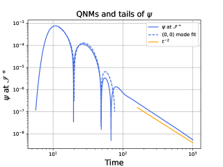
Figure 10: Here we plot the rescaled scalar field at future null infinity as a function of time from a nonlinear evolution starting with constraint solved initial data (details in main text) that are a scalar field perturbation of Schwarzschild. Here we employed the height-function Jacobians. The initial perturbation in this case is sufficiently small that the resulting picture rapidly resembles closely that from the Cowling approximation. In the first phase we have fit the fundamental spherical QNM [66] with complex frequency $\omega M\simeq 0.11+0.10i$. Later the field decays as a $t^{-2}$ power-law. With eikonal Jacobians the behavior is qualitatively similar although we leave a detailed examination of the frequencies, which requires further post-processing, to future work.

IV Conclusions

Continuing our research program towards the inclusion of future null infinity in the computational domain in full 3d numerical relativity, here we presented an implementation of spherical GR in GHG that uses the dual-foliation formalism to get all the way out. The strategy is to take the evolved variables to be equivalent to those that would be solved for in the standard Cauchy problem, subjected to a rescaling to obtain non-trivial $O(1)$ quantities, and then to change to compactified hyperboloidal coordinates. In this way, the hope is to extend the computational domain to null infinity in a manner that leaves the numerical treatment in the strong-field region absolutely unchanged, and in the future without symmetry. We examined a broad suite of initial data, including gauge waves, constraint violating and satisfying configurations. We considered spacetimes with a regular center and dynamical black holes, in which case we use the excision method to remove the interior. In all cases our initial data were posed on hyperboloidal slices. The coordinate transformation was managed either by the use of a height-function or by solving the eikonal equation, both with a given radial compactification containing a parameter $1<n\leq 2$ that controls how fast the transformation is made. We have examples in which the compactification takes effect immediately from the origin, and others which employ hyperboloidal layers, where it takes effect only further out.

To construct constraint satisfying data from regular equations with scalar field matter, we treated the overall solution to be a perturbation of the Minkowski or Schwarzschild spacetimes, taking suitable initial data for the gauge drivers. In both cases, those corrections turned out to possess a geometrical and physical interpretation in terms of the Misner-Sharp mass. We believe that this technique can be generalized, first to drop simplifying assumptions within spherical symmetry, but also to full $3$d, both of which are kept for future work.

We find convincing evidence for numerical convergence across the entire suite of spacetimes we considered. Although we did not make any push for precision here, for physical initial data we did find good compatibility vis-à-vis expected frequencies and rates, for instance in QNMs and Price decay.

It is gratifying to see the line of reasoning developed across the direct precursors to this study work bear fruit in full GR, even if only in the spherical setting. In brief, in [35] it was observed that to obtain equations of motion regular enough to treat on compactified hyperboloidal slices, the coordinate light-speed variable $C_{+}$ needs to display decay beyond that expected for solutions of the wave-equation. It was then argued in [39] that this could be achieved in the GHG formulation, even when the constraints are violated, by appropriate constraint addition to the field equations. In plain harmonic gauge it is known that either slow decay of the stress-energy tensor or the presence of gravitational waves serve as an obstruction to decay of the metric components. In [41] it was observed that this shortcoming of the gauge can be overcome by the use of carefully chosen gauge source functions. In parallel, numerical studies were performed with model problems with the same asymptotics as in GR in GHG. These taught us first [43] a convenient choice of reduction variables, second [44] the importance of using truncation error matching at null infinity, and third [45] that the general strategy to suppress log-terms is indeed viable in practice.

The interplay between the mathematical and numerical works has also been important in getting to this stage. For instance, in [41] the suggestion was to force improved asymptotics for all metric components except for those associated with gravitational waves. In practice however, with the GBUF model problem, it was found that this approach would make convergence in the numerics difficult. (For this reason we have worked here with $p=0$ in (37) for the $C_{-}$ variable). Evidently, all of these ingredients played an important role in treating spherical GR.

Although the results presented are an important milestone in our research program, open questions remain both in spherical symmetry and more generally. So far we have done nothing to chase down sharp conditions in the required asymptotics of our method. In our current setup we insist, for instance, on hyperboloidal initial data such that the radiation field from our scalar matter is $O(1)$ at $\mathscr{I}^{+}$. But it is known even in the Minkowski spacetime that ‘reasonable’ Cauchy data for the wave equation can result in solutions with logarithmically growing radiation fields [67, 68, 69]. In the future we wish to understand more clearly the class of data that allows for the inclusion of $\mathscr{I}^{+}$ in the computational domain, and how that class sits within the broader choice that allows analogous growth in the radiation fields. It would be good also to formulate conditions, ideally necessary and sufficient, on the choice of gauge that would allow for the inclusion of $\mathscr{I}^{+}$ in the computational domain, even within the better class of data. On a more technical level we wish to achieve successful numerical evolutions with the most aggressive compactification parameter $n=2$, to work without the first order reduction, and to switch to higher order and pseudospectral methods. Despite these questions, in view of the 3d toy-model results of [45] and those presented here for spherical GR, we believe that the essential pieces are now in place to achieve, in the near-term, the goal of 3d numerical evolutions of full GR in GHG on compactified hyperboloidal slices.

V Acknowledgements

The authors thank Sukanta Bose, Miguel Duarte, Justin Feng, Edgar Gasperin, Prayush Kumar and Anil Zenginoğlu for helpful discussions and or comments on the manuscript.

The Mathematica notebooks associated with this work can be found at [47].

The authors thank FCT for financial support through Project No. UIDB/00099/2020 and for funding with DOI 10.54499/DL57/2016/CP1384/CT0090, as well as IST-ID through Project No. 1801P.00970.1.01.01. This work was partially supported by the ICTS Knowledge Exchange Grants owned by the ICTS Director and Prayush Kumar, Ashok and Gita Vaish Early Career Faculty Fellowship owned by Prayush Kumar at the ICTS. Part of the computational work was performed on the Sonic cluster at ICTS. SG’s research was supported by the Department of Atomic Energy, Government of India, under project no. RTI4001, Infosys-TIFR Leading Edge Travel Grant, Ref. No.: TFR/Efund/44/Leading Edge TG (R-2)/8/, and the University Grants Commission (UGC), India Senior Research Fellowship. Part of this work was done at the University of the Balearic Islands (UIB), Spain, the Department of Mathematics at the University of Valencia and the Astrophysical and Cosmological Relativity department at the Albert Einstein Institute, aka the Max-Planck Institute for Gravitational Physics in Potsdam-Golm. SG thanks Sascha Husa, Isabel Cordero Carrión and Alessandra Buonanno for local hospitality and travel support at these institutions.

References

- Wald [1984] R. M. Wald, General relativity (The University of Chicago Press, Chicago, 1984).
- Winicour [2012] J. Winicour, Characteristic evolution and matching, Living Rev. Relativity 15, 2 (2012), [Online article].
- Moxon et al. [2020] J. Moxon, M. A. Scheel, and S. A. Teukolsky, Improved Cauchy-characteristic evolution system for high-precision numerical relativity waveforms, Phys. Rev. D 102, 044052 (2020), arXiv:2007.01339 [gr-qc] .
- Moxon et al. [2021] J. Moxon, M. A. Scheel, S. A. Teukolsky, N. Deppe, N. Fischer, F. Hébert, L. E. Kidder, and W. Throwe, The SpECTRE Cauchy-characteristic evolution system for rapid, precise waveform extraction (2021), arXiv:2110.08635 [gr-qc] .
- Ma et al. [2023] S. Ma, J. Moxon, M. A. Scheel, K. C. Nelli, N. Deppe, M. S. Bonilla, L. E. Kidder, P. Kumar, G. Lovelace, W. Throwe, and N. L. Vu, Fully relativistic three-dimensional Cauchy-characteristic matching, arXiv:2308.10361 (2023), arXiv:2308.10361 [gr-qc] .
- Giannakopoulos et al. [2020] T. Giannakopoulos, D. Hilditch, and M. Zilhão, Hyperbolicity of general relativity in bondi-like gauges, Phys. Rev. D 102, 064035 (2020), arXiv:2007.06419 [gr-qc] .
- Giannakopoulos et al. [2022] T. Giannakopoulos, N. T. Bishop, D. Hilditch, D. Pollney, and M. Zilhao, Gauge structure of the Einstein field equations in Bondi-like coordinates, Phys. Rev. D 105, 084055 (2022), arXiv:2111.14794 [gr-qc] .
- Giannakopoulos et al. [2023] T. Giannakopoulos, N. T. Bishop, D. Hilditch, D. Pollney, and M. Zilhão, Numerical convergence of model Cauchy-Characteristic Extraction and Matching, arXiv:2306.13010 (2023), arXiv:2306.13010 [gr-qc] .
- Gundlach [2024] C. Gundlach, Simulations of gravitational collapse in null coordinates: III. Hyperbolicity, (2024), arXiv:2404.16720 [gr-qc] .
- Friedrich [1981] H. Friedrich, On the Regular and the Asymptotic Characteristic Initial Value Problem for Einstein’s Vacuum Field Equations, Proc. R. Soc. Lond. A 375, 169 (1981).
- Friedrich [1983] H. Friedrich, Cauchy problems for the conformal vacuum field equations in general relativity, Communications in Mathematical Physics 91, 445 (1983).
- Friedrich [1986] H. Friedrich, On the existence of n-geodesically complete or future complete solutions of Einstein’s field equations with smooth asymptotic structure, Comm. Math. Phys. 107, 587 (1986).
- Zenginoglu [2011] A. Zenginoglu, Hyperboloidal layers for hyperbolic equations on unbounded domains, J. Comput. Phys. 230, 2286 (2011), arXiv:1008.3809 [math.NA] .
- Macedo et al. [2018] R. P. Macedo, J. L. Jaramillo, and M. Ansorg, Hyperboloidal slicing approach to quasinormal mode expansions: The reissner-nordström case, Physical Review D 98, 124005 (2018).
- Macedo [2020] R. P. Macedo, Hyperboloidal framework for the kerr spacetime, Classical and Quantum Gravity 37, 065019 (2020).
- Macedo et al. [2022] R. P. Macedo, B. Leather, N. Warburton, B. Wardell, and A. Zenginoğlu, Hyperboloidal method for frequency-domain self-force calculations, Physical Review D 105, 104033 (2022).
- Valiente-Kroon [2016] J.-A. Valiente-Kroon, Conformal Methods in General Relativity (Cambridge University Press, Cambridge, 2016).
- Frauendiener [2004] J. Frauendiener, Conformal infinity, Living Rev. Relativity 7 (2004).
- Beyer et al. [2020a] F. Beyer, J. Frauendiener, and J. Hennig, Explorations of the infinite regions of spacetime, Int. J. Mod. Phys. D 29, 2030007 (2020a), arXiv:2005.11936 [gr-qc] .
- Frauendiener and Stevens [2021] J. Frauendiener and C. Stevens, The non-linear perturbation of a black hole by gravitational waves. i. the bondi–sachs mass loss, Classical and Quantum Gravity 38, 194002 (2021).
- Frauendiener and Stevens [2023] J. Frauendiener and C. Stevens, The non-linear perturbation of a black hole by gravitational waves. ii. quasinormal modes and the compactification problem, Classical and Quantum Gravity 40, 125006 (2023).
- Frauendiener et al. [2024] J. Frauendiener, A. Goodenbour, and C. Stevens, The non-linear perturbation of a black hole by gravitational waves. iii. newman–penrose constants, Classical and Quantum Gravity 41, 065005 (2024).
- Zenginoglu [2007] A. Zenginoglu, A conformal approach to numerical calculations of asymptotically flat spacetimes, Ph.D. thesis, Potsdam U., Inst. of Math. (2007), arXiv:0711.0873 [gr-qc] .
- Zenginoglu [2008] A. Zenginoglu, Hyperboloidal evolution with the Einstein equations, Class. Quant. Grav. 25, 195025 (2008), arXiv:0808.0810 [gr-qc] .
- Moncrief and Rinne [2009] V. Moncrief and O. Rinne, Regularity of the Einstein Equations at Future Null Infinity, Class.Quant.Grav. 26, 125010 (2009), arXiv:0811.4109 [gr-qc] .
- Rinne [2010] O. Rinne, An axisymmetric evolution code for the Einstein equations on hyperboloidal slices, Class. Quant. Grav. 27, 035014 (2010), arXiv:0910.0139 [gr-qc] .
- Rinne and Moncrief [2013] O. Rinne and V. Moncrief, Hyperboloidal Einstein-matter evolution and tails for scalar and Yang-Mills fields, Class.Quant.Grav. 30, 095009 (2013), arXiv:1301.6174 [gr-qc] .
- Bardeen et al. [2011] J. M. Bardeen, O. Sarbach, and L. T. Buchman, Tetrad formalism for numerical relativity on conformally compactified constant mean curvature hypersurfaces, Phys. Rev. D 83, 104045 (2011), arXiv:1101.5479 [gr-qc] .
- Morales and Sarbach [2017] M. D. Morales and O. Sarbach, Evolution of scalar fields surrounding black holes on compactified constant mean curvature hypersurfaces, Phys. Rev. D 95, 044001 (2017), arXiv:1609.05756 [gr-qc] .
- Vañó-Viñuales et al. [2015] A. Vañó-Viñuales, S. Husa, and D. Hilditch, Spherical symmetry as a test case for unconstrained hyperboloidal evolution, Class. Quant. Grav. 32, 175010 (2015), arXiv:1412.3827 [gr-qc] .
- Vañó-Viñuales [2015] A. Vañó-Viñuales, Free evolution of the hyperboloidal initial value problem in spherical symmetry, Ph.D. thesis, U. Illes Balears, Palma (2015), arXiv:1512.00776 [gr-qc] .
- Vañó-Viñuales and Husa [2018] A. Vañó-Viñuales and S. Husa, Spherical symmetry as a test case for unconstrained hyperboloidal evolution II: gauge conditions, Class. Quant. Grav. 35, 045014 (2018), arXiv:1705.06298 [gr-qc] .
- Vañó Viñuales and Valente [2024] A. Vañó Viñuales and T. Valente, Height-function-based 4D reference metrics for hyperboloidal evolution, (2024), arXiv:2408.08952 [gr-qc] .
- Hilditch [2015] D. Hilditch, Dual Foliation Formulations of General Relativity, arXiv:1509.02071 (2015), arXiv:1509.02071 [gr-qc] .
- Hilditch et al. [2018] D. Hilditch, E. Harms, M. Bugner, H. Rüter, and B. Brügmann, The evolution of hyperboloidal data with the dual foliation formalism: Mathematical analysis and wave equation tests, Class. Quant. Grav. 35, 055003 (2018), arXiv:1609.08949 [gr-qc] .
- Hörmander [1987] L. Hörmander, The lifespan of classical solutions of non-linear hyperbolic equations, in Pseudo-Differential Operators: Proceedings of a Conference held in Oberwolfach, February 2–8, 1986 (Springer Berlin Heidelberg, Berlin, Heidelberg, 1987) pp. 214–280.
- [37] L. Hörmander, Lectures on Nonlinear Hyperbolic Differential Equations, Mathématiques et Applications.
- Lindblad and Rodnianski [2003] H. Lindblad and I. Rodnianski, The weak null condition for Einstein’s equations, Comptes Rendus Mathematique 336, 901 (2003).
- Gasperín and Hilditch [2019] E. Gasperín and D. Hilditch, The Weak Null Condition in Free-evolution Schemes for Numerical Relativity: Dual Foliation GHG with Constraint Damping, Class. Quant. Grav. 36, 195016 (2019), arXiv:1812.06550 [gr-qc] .
- Duarte et al. [2021] M. Duarte, J. Feng, E. Gasperín, and D. Hilditch, High order asymptotic expansions of a good–bad–ugly wave equation, Classical and Quantum Gravity 38, 145015 (2021), arXiv:2101.07068 [gr-qc] .
- Duarte et al. [2022] M. Duarte, J. C. Feng, E. Gasperin, and D. Hilditch, Peeling in generalized harmonic gauge, Class. Quant. Grav. 39, 215003 (2022), arXiv:2205.09405 [gr-qc] .
- Duarte et al. [2023a] M. Duarte, J. C. Feng, E. Gasperín, and D. Hilditch, Regularizing dual-frame generalized harmonic gauge at null infinity, Class. Quant. Grav. 40, 025011 (2023a), arXiv:2206.13661 [gr-qc] .
- Gasperín et al. [2020] E. Gasperín, S. Gautam, D. Hilditch, and A. Vañó Viñuales, The Hyperboloidal Numerical Evolution of a Good-Bad-Ugly Wave Equation, Class. Quant. Grav. 37, 035006 (2020), arXiv:1909.11749 [gr-qc] .
- Gautam et al. [2021] S. Gautam, A. Vañó Viñuales, D. Hilditch, and S. Bose, Summation by Parts and Truncation Error Matching on Hyperboloidal Slices, Phys. Rev. D 103, 084045 (2021), arXiv:2101.05038 [gr-qc] .
- Peterson et al. [2023] C. Peterson, S. Gautam, I. Rainho, A. Vañó Viñuales, and D. Hilditch, 3D evolution of a semilinear wave model for the Einstein field equations on compactified hyperboloidal slices, Phys. Rev. D 108, 024067 (2023), arXiv:2303.16190 [gr-qc] .
- Misner and Sharp [1964] C. W. Misner and D. H. Sharp, Relativistic equations for adiabatic, spherically symmetric gravitational collapse, Phys. Rev. 136, B571 (1964).
- [47] https://doi.org/10.5281/zenodo.13685353.
- Calabrese et al. [2006] G. Calabrese, C. Gundlach, and D. Hilditch, Asymptotically null slices in numerical relativity: Mathematical analysis and spherical wave equation tests, Class.Quant.Grav. 23, 4829 (2006), arXiv:gr-qc/0512149 [gr-qc] .
- Vañó Viñuales [2023] A. Vañó Viñuales, Spherically symmetric black hole spacetimes on hyperboloidal slices, Front. Appl. Math. Stat., Sec. Statistical and Computational Physics 9, 10.3389/fams.2023.1206017 (2023), arXiv:2304.05384 [gr-qc] .
- Bondi et al. [1962] H. Bondi, M. G. J. van der Burg, and A. W. K. Metzner, Gravitational waves in general relativity. vii. waves from axi-symmetric isolated systems, Proceedings of the Royal Society of London. Series A, Mathematical and Physical Sciences 269, 21 (1962).
- Friedrich [2005] H. Friedrich, On the non-linearity of the subsidiary systems, Class. Quant. Grav. 22, L77 (2005), arXiv:gr-qc/0504129 .
- Lindblom et al. [2006] L. Lindblom, M. A. Scheel, L. E. Kidder, R. Owen, and O. Rinne, A new generalized harmonic evolution system, Class. Quant. Grav. 23, S447 (2006), gr-qc/0512093 .
- Beyer et al. [2017] F. Beyer, L. Escobar, and J. Frauendiener, Asymptotics of solutions of a hyperbolic formulation of the constraint equations, Class. Quant. Grav. 34, 205014 (2017), arXiv:1706.06700 [gr-qc] .
- Nakonieczna et al. [2021] A. Nakonieczna, L. Nakonieczny, and I. Rácz, Black hole initial data by numerical integration of the parabolic–hyperbolic form of the constraints, Int. J. Mod. Phys. D 30, 2150111 (2021), arXiv:1712.00607 [gr-qc] .
- Beyer et al. [2019] F. Beyer, L. Escobar, J. Frauendiener, and J. Ritchie, Numerical construction of initial data sets of binary black hole type using a parabolic-hyperbolic formulation of the vacuum constraint equations, Class. Quant. Grav. 36, 175005 (2019), arXiv:1903.06329 [gr-qc] .
- Csukás and Rácz [2020] K. Csukás and I. Rácz, Numerical investigations of the asymptotics of solutions to the evolutionary form of the constraints, Class. Quant. Grav. 37, 155006 (2020), arXiv:1911.02900 [gr-qc] .
- Beyer et al. [2020b] F. Beyer, J. Frauendiener, and J. Ritchie, Asymptotically flat vacuum initial data sets from a modified parabolic-hyperbolic formulation of the Einstein vacuum constraint equations, Phys. Rev. D 101, 084013 (2020b), arXiv:2002.06759 [gr-qc] .
- Beyer and Ritchie [2022] F. Beyer and J. Ritchie, Asymptotically hyperboloidal initial data sets from a parabolic–hyperbolic formulation of the Einstein vacuum constraints, Class. Quant. Grav. 39, 145012 (2022), arXiv:2104.10290 [gr-qc] .
- Csukás and Rácz [2023] K. Csukás and I. Rácz, Is it possible to construct asymptotically flat initial data using the evolutionary forms of the constraints?, Phys. Rev. D 107, 084013 (2023), arXiv:2302.00590 [gr-qc] .
- Evans [1984] C. R. Evans, A Method for Numerical Relativity: Simulation of Axisymmetric Gravitational Collapse and Gravitational Radiation Generation, Ph.D. thesis, University of Texas at Austin (1984).
- Gundlach et al. [2013] C. Gundlach, J. M. Martin-Garcia, and D. Garfinkle, Summation by parts methods for spherical harmonic decompositions of the wave equation in any dimensions, Class. Quant. Grav. 30, 145003 (2013), arXiv:1010.2427 [math.NA] .
- Hemberger et al. [2013] D. A. Hemberger, M. A. Scheel, L. E. Kidder, B. Szilagyi, G. Lovelace, et al., Dynamical Excision Boundaries in Spectral Evolutions of Binary Black Hole Spacetimes, Class.Quant.Grav. 30, 115001 (2013), arXiv:1211.6079 [gr-qc] .
- Bhattacharyya et al. [2021] M. K. Bhattacharyya, D. Hilditch, K. Rajesh Nayak, S. Renkhoff, H. R. Rüter, and B. Brügmann, Implementation of the dual foliation generalized harmonic gauge formulation with application to spherical black hole excision, Phys. Rev. D 103, 064072 (2021), arXiv:2101.12094 [gr-qc] .
- Alcubierre [2008] M. Alcubierre, Introduction to 3+1 Numerical Relativity (Oxford University Press, Oxford, 2008).
- Vañó-Viñuales and Husa [2015] A. Vañó-Viñuales and S. Husa, Unconstrained hyperboloidal evolution of black holes in spherical symmetry with GBSSN and Z4c, Proceedings, Spanish Relativity Meeting: Almost 100 years after Einstein Revolution (ERE 2014), J. Phys. Conf. Ser. 600, 012061 (2015), arXiv:1412.4801 [gr-qc] .
- Berti et al. [2009] E. Berti, V. Cardoso, and A. O. Starinets, Quasinormal modes of black holes and black branes, Class. Quant. Grav. 26, 163001 (2009), arXiv:0905.2975 [gr-qc] .
- Duarte et al. [2023b] M. Duarte, J. Feng, E. Gasperin, and D. Hilditch, The good-bad-ugly system near spatial infinity on flat spacetime, Class. Quant. Grav. 40, 055002 (2023b), arXiv:2209.12247 [gr-qc] .
- Gasperin [2024] E. Gasperin, Polyhomogeneous spin-0 fields in Minkowski space–time, Phil. Trans. Roy. Soc. Lond. A 382, 20230045 (2024), arXiv:2306.15355 [gr-qc] .
- Gasperín et al. [2024] E. Gasperín, M. Magdy, and F. C. Mena, Asymptotics of spin-0 fields and conserved charges on n-dimensional minkowski spaces (2024), arXiv:2408.03389 [gr-qc] .