LibMOON: A Gradient-based MultiObjective OptimizatioN Library in PyTorch

Abstract

Multiobjective optimization problems (MOPs) are prevalent in machine learning, with applications in multi-task learning, learning under fairness or robustness constraints, etc. Instead of reducing multiple objective functions into a scalar objective, MOPs aim to optimize for the so-called Pareto optimality or Pareto set learning, which involves optimizing more than one objective function simultaneously, over models with thousands / millions of parameters. Existing benchmark libraries for MOPs mainly focus on evolutionary algorithms, most of which are zeroth-order / meta-heuristic methods that do not effectively utilize higher-order information from objectives and cannot scale to large-scale models with thousands / millions of parameters. In light of the above gap, this paper introduces LibMOON, the first multiobjective optimization library that supports state-of-the-art gradient-based methods, provides a fair benchmark, and is open-sourced for the community.

Keywords Mathematical tools  $\cdot$ Multiobjective optimization  $\cdot$ Pareto set learning  $\cdot$ Bayesian optimization

1 Introduction

MultiObjective Optimization problems (MOPs) are ubiquitous in machine learning. For instance, trustworthy machine learning (TML) includes fairness problems balancing the fairness level and the accuracy level [1, 2]; in robotics, it is necessary to balance several objectives (e.g., forward speed and energy consumption)  [3, 4]; similarly, recommendation systems face potentially conflicting objectives, such as novelty, accuracy, and diversity [5, 6, 7]. For all the applications above, the underlying optimization problem involves an MOP with $m$ objectives and can be (informally) defined as:

$$\min_{\theta}{\bm{L}}({\bm{\theta}})=(L_{1}({\bm{\theta}}),\ldots,L_{m}({\bm{\theta}})),$$ (1)

where $L_{1}({\bm{\theta}}),\ldots,L_{m}({\bm{\theta}})$ denote $m$ (potentially) conflicting objectives and we denote the size of the model parameter as $N\coloneqq|{\bm{\theta}}|$. Note that as informally defined above, Equation 1 is a vector optimization problem that does not necessarily admit a total ordering.

For non-trivial multiobjective problems, no single solution can attain the minimum of all objectives simultaneously. To compare two solutions for an MOP, we introduce the concepts of dominance and Pareto optimality [8]. Dominance occurs when solution ${\bm{\theta}}^{(a)}$ satisfies $L_{i}({\bm{\theta}}^{(a)})\leq L_{i}({\bm{\theta}}^{(b)})$ for all $1\leq i\leq m$, with at least one strict inequality $L_{j}({\bm{\theta}}^{(a)})<L_{j}({\bm{\theta}}^{(b)})$. A solution is Pareto optimal if no other solution in the feasible region dominates it. The set of all Pareto optimal solutions is the Pareto set (PS), and its image is the Pareto front (PF).

Over the last few decades, multiobjective evolutionary algorithms (MOEAs) emerged as a widely used methodology for addressing MOPs. Due to their population-level designs, MOEAs can identify a diverse set of Pareto optimal solutions that approximate and represent the entire PF of a given MOP. Several libraries have emerged as standard platforms for fair comparison of MOEAs, including PlatEMO [9] (in Matlab supporting over 160 MOEAs), Pagmo [10] (in C++), and Pymoo [11] (in Python).

Compared to MOEAs, gradient-based multiobjective optimization (MOO) methods are particularly suitable designed for large-scale machine learning tasks involving thousands to millions of neural network parameters. While these methods can find Pareto stationary solutions—solutions that cannot be locally improved in any objective—they are also effective approximators of Pareto solutions for nonconvex models, including deep neural networks [12].

In this paper, we roughly divide recent gradient-based MOO methods into two main groups. The first one focuses on finding a finite set of Pareto solutions to approximately represent the entire PF. Examples include Upper Bounded Multiple Gradient Descent Algorithm (MGDA-UB) [13] and Exact Pareto Optimization (EPO) [14]. The second, known as Pareto set learning (PSL) [15, 16, 17], develops a single neural model parameterized by ${\bm{\phi}}$ to represent the entire Pareto set. Since the parameter space of ${\bm{\phi}}$ is large, thus PSL is usually optimized by gradient-based methods.

With the growing use of gradient-based MOO methods in neural networks [13, 18, 4, 16, 19, 20, 21], there is a pressing need for a standard library to benchmark comparisons and developments. To fulfill this demand, we introduce LibMOON, a gradient-based Multi-Objective Optimization Library supporting over twenty state-of-the-art methods.

We summarize our contributions as follows:

1. We propose the first modern gradient-based MOO library, called LibMOON. LibMOON is implemented under the PyTorch framework [22] and carefully designed to support GPU acceleration. LibMOON supports synthetic problems and a wide range of real-world multiobjective machine learning tasks (e.g., fair classification and multiobjective classification problems).

2. LibMOON supports over twenty state-of-the-art (SOTA) gradient-based MOO methods for constructing Pareto optimal solution sets, including those using finite solutions to approximate the whole PS/PF [14, 19], PSL methods [16, 15] aimed at approximating the entire Pareto set with a single neural network, and MOBO methods that designed to avoid frequent function evaluations.

3. LibMOON has already been open-sourced at https://github.com/xzhang2523/libmoon with document at https://libmoondocs.readthedocs.io/en/latest/, offering a reliable platform for comparing SOTA gradient-based MOO approaches and providing standard multiobjective testing benchmarks. Beyond examining its source code, LibMOON can be installed via pip install libmoon as an off-the-shelf gradient-based multiobjective tool.

Notation.

In this paper, bold letters represent vectors (e.g., ${\bm{\lambda}}$ for preference vectors, ${\bm{L}}()$ for vector objective functions), while non-bold letters represent scalars. The number of objectives is denoted by $m$, and $K$ represents the size of finite solution set. The preference vector ${\bm{\lambda}}$ lies in the $m$-dim simplex (${\bm{\Delta}}_{m}$), satisfying $\sum_{i=1}^{m}\lambda_{i}=1$ and $\lambda_{i}\geq 0$. The decision network parameter ${\bm{\theta}}$ has a size of $n$. Refer to Table 12 for the full notation table.

2 Related works

In this section, we review some methods for gradient-based multiobjective optimization in Section 2.1 and existing multiobjective optimization libraries in Section 2.2.

2.1 Gradient-based multiobjective optimization

Gradient-based MOO has a long research history. For instance, the famous convex optimization book [23][Chap 4] discusses how to use linear scalarization to convert MOO into a single-objective optimization (SOO) problem. However, in the last several decades, gradient-based methods were not a mainstream for MOO, with evolutionary algorithms (MOEAs) being more prevalent due to their ability to maintain a population, which is inherently suitable to approximate the Pareto set and avoid local optimal solutions. However, gradient-based MOO has gained growing popularity very recently with their applications in (deep) machine learning. A seminal work in this field is MGDA-UB [13], which introduced MOO concepts into deep learning by framing an MTL problem as an MOO. Since then, numerous approaches such as EPO [14], Pareto MultiTask learning (PMTL) [18], MOO with Stein Variational Gradient Descent (MOO-SVGD) [19], and methods for learning the entire Pareto set [15, 16, 24, 25, 26], have emerged. This paper categorized these methods by two main classes and implement these methods in a standard manner.

2.2 Multiobjective optimization libraries

A number of multiobjective libraries exist before our work. The difference between LibMOON and previous libraries is that LibMOON is designed to support gradient-based MOO methods. Comparisons with previous is provided in Table 1.

LibMTL [27]. LibMTL is a Python-based library for multitask learning. The key difference between LibMOON and LibMTL is that LibMTL focuses on finding a single network to benefit all tasks, such as calculating a benign updating direction or optimizing a network architecture. In contrast, LibMOON addresses inherent trade-offs in machine learning problems, where improving one objective inevitably worsens others, and explores the distribution of Pareto solutions.

jMetal [28]. jMetal is a comprehensive Java framework designed for multi-objective optimization, leveraging the power of metaheuristics. It offers a highly flexible and extensible platform, making it accessible for users across various domains. With its user-friendly interface and robust architecture, jMetal has become a popular choice for researchers and practitioners in diverse application areas.

Pymoo [29]. Pymoo is a Python-based framework for multiobjective optimization problems with many local optima. Pymoo supports mainstream MOEA methods such as NSGA-II [30], NSGA-III [31, 32], MOEA/D [33], and SMS-EMOA [34]. Pymoo allows flexible algorithm customization with user-defined operators and includes tools for exploratory analysis and data visualization. It also offers multi-criteria decision-making strategies to help users select optimal solutions from the Pareto set.

PlatEMO [9]. PlatEMO is a MATLAB-based multiobjective optimization tool supporting over 160 evolutionary algorithms and a comprehensive set of test problems. It supports diverse problem types, including sparse, high-cost, large-scale, and multimodal. PlatEMO includes performance metrics for evaluating optimization efficacy and offers tools for visualization and interaction during the optimization process.

Pagmo [10]. Pagmo, a C++ library, executes massively parallel multiobjective global optimization using efficient evolutionary algorithms and gradient-based techniques like simplex, SQP, and interior-point methods. It supports concurrent algorithm execution and inter-algorithm collaboration through asynchronous generalized island models, addressing a wide range of optimization challenges, including constrained, unconstrained, single-objective, multiobjective, continuous, integer, stochastic, and deterministic problems.

EvoTorch [35] and EvoX [36]. EvoTorch accelerates evolutionary algorithms in PyTorch, while EvoX scales them to large, complex problems with GPU-accelerated parallel execution for single and multiobjective tasks, including synthetic and reinforcement learning. These libraries highlight a trend toward using GPU parallelization to manage larger problem scales and decision variables, which is also of the interest of this paper. This work focuses on creating a platform for efficient gradient-based multiobjective methods to solve large-scale machine learning problems in PyTorch.

Table 1: Comparison of different libraries and frameworks.

Name	Language	Publication	Installable	Key Feature
Pymoo	Python	2020	✓	Evolutionary computation (EC)
jMetal	Java	2011	✓	EC and meta-heuristics
PlatEMO	Matlab	2017	×	EC and meta-heuristics
Pagmo	C++	2020	×	Global optimization
LibMTL	Python	2023	✓	A single solution benefiting all tasks
EvoTorch	Python	NA	✓	GPU acceleration for EC
EvoX	Python	2024	✓	GPU acceleration for EC
LibMOON	Python	NA	✓	GPU accelerated gradient-based MOO solvers

3 LibMOON: A gradient-based MOO library in PyTorch

This section introduces LibMOON . We first introduce its framework in Section 3.1, and briefly introducing its supporting problems and metrics. Then we introduce supported solvers in Sections 3.2, 3.3 and 3.4.

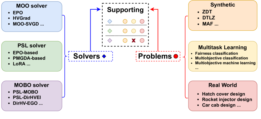
Figure 1: The Framework of LibMOON: LibMOON addresses synthetic, real-world and MTL problems with three categories of solvers: MOO, PSL and MOBO solvers.

3.1 Framework

Figure 1 demonstrates the framework of the proposed LibMOON library. LibMOON supports three categories of solvers: MOO solvers aiming to find a finite set of Pareto solutions satisfying certain requirements, PSL solvers aiming to learn whole PS with a single model, and MOBO solvers aiming to solve expensive problems. Each solver category is designed highly modulized and new solvers are easy to plugin LibMOON by rewriting only a small portion of code, e.g., the specific way of gradient manipulations . MOO and PSL solvers support all synthetic, MTL, and realworld (RE) problems, while MOBO solvers support synthetic and RE problems.

Table 2: Supported multiobjective machine learning problems in LibMOON.

Method	$L_{1}$	$L_{2}$
Fairness classification [37]	Binary cross entropy	DEO
Multiobjective classification [18]	Cross entropy loss BR	Cross entropy loss UL
MO machine learning [20]	Mean square loss	Mean square loss
MO distribution alignment	Similarity 1	Similarity 2

• DEO [38]: Difference of Equality of Opportunity.

Supported problems.

LibMOON currently supports three categories of methods, synthetic problems, MTL problems, and RE problems.

Supported metrics.

LibMOON supports a wide range of metrics namely, (1) hypervolume (HV), (2) inverted general distance (IGD), (3) fill distance (FD), (4) minimal distance ($\mathrm{l}_{\min}$), (5) smooth minimal distance ($\mathrm{sl}_{\min}$), (5) Spacing, (6) Span, (7) penalty-based intersection (PBI), (8) inner product (IP), (9) cross angle ($\vartheta$). Full descriptions of these indicators are provided in Table 13.

3.2 MOO solvers

Table 3: Supported finite Pareto solution solvers, their properties, and time complexity for one iteration.

Method	Property	Paper	Complexity	Pref. based
EPO [14]	Exact solutions	paper	$O(m^{2}nK)$	✓
HVGrad [39]	Maximal HV solutions	paper	$O(m^{2}nK^{2})$	×
MGDA-UB [13]	Arbitrary solutions	paper	$O(m^{2}nK)$	×
MOO-SVGD [19]	Diverse solutions	paper	$O(m^{2}nK^{2})$	×
PMGDA [40]	Specific solutions	paper	$O(m^{2}nK)$	✓
PMTL [18]	Sector-constrained solutions	paper	$O(m^{2}nK^{2})$	×
Random [41]	Arbitrary solutions	paper	$O(m^{2}nK)$	×
Agg-LS [42]	Convex hull solutions	book	$O(mnK)$	✓
Agg-Tche [33]	Exact solutions	paper	$O(mnK)$	✓
Agg-mTche [43]	Exact solutions	paper	$O(mnK)$	✓
Agg-PBI [33]	Approximate exact solutions	paper	$O(mnK)$	✓
Agg-COSMOS [37]	Approximate exact solutions	paper	$O(mnK)$	✓
Agg-SmoothTche [25]	Fast approximate exact solutions	paper	$O(mnK)$	✓

• $m$: number of objectives. $n$: number of decision variables. $K$: number of subproblems.

Aggregation function.

To find Pareto solutions, a straightforward way is to use some aggregation functions $g_{\bm{\lambda}}^{\mathrm{agg}}():\mathbb{R}^{m}\to\mathbb{R}$ to convert a multi-objective problem (MOP) into a single-objective optimization problem (SOP). Aggregation function based methods aim to optimize the following objective function:

$$\min_{\bm{\theta}}g_{\bm{\lambda}}^{\mathrm{agg}}({\bm{L}}({\bm{\theta}})),$$ (2)

where ${\bm{L}}({\bm{\theta}})$ represents an objective vector and $g_{\bm{\lambda}}^{\mathrm{agg}}()$ is an aggregation function determined by a preference vector ${\bm{\lambda}}$. If $g_{\bm{\lambda}}^{\mathrm{agg}}()$ is decreasing with respect to ${\bm{L}}({\bm{\theta}})$ (i.e., $g_{\bm{\lambda}}^{\mathrm{agg}}({\bm{L}}({\bm{\theta}}^{(a)}))<g_{\bm{\lambda}}^{\mathrm{agg}}({\bm{L}}({\bm{\theta}}^{(b)}))$ when ${\bm{L}}_{i}({\bm{\theta}}^{(a)})\leq{\bm{L}}_{i}({\bm{\theta}}^{(b)})$ for all $i$ with at least one strict inequality), the optimal solution of Equation 2 corresponds to a Pareto optimal solution of the original MOP (Equation 1) [42].

The linear scalarization (LS) function, $g_{\bm{\lambda}}^{\mathrm{agg}}({\bm{L}}({\bm{\theta}}))=\sum_{i=1}^{m}\lambda_{i}L_{i}({\bm{\theta}})$, is the most commonly used aggregation function. Other notable functions include the (Smooth) Tchebycheff (Tche) [25, 42], modified Tchebycheff (mTche) [43], Penalty-Based Intersection (PBI) [33], and COSMOS [37]. For detailed formulations, see Appendix A. Aggregation-based methods can be efficiently optimized in LibMOON using single objective backpropagation. Aggregation-based method update the parameter ${\bm{\theta}}$ iteratively as follows:

$${\bm{\theta}}\xleftarrow{}{\bm{\theta}}-\eta{\bm{d}}={\bm{\theta}}-\eta\frac{\partial g_{\bm{\lambda}}^{\mathrm{agg}}({\bm{L}}({\bm{\theta}}))}{\partial{\bm{\theta}}},$$ (3)

where ${\bm{d}}$ is called an updating direction.

Generalized aggregation function.

In addition to optimizing the single-objective aggregation function, a number of gradient manipulation methods adjust gradients and compute update directions to ensure solutions satisfy specific properties. These methods can be summarized as follows: the update direction ${\bm{d}}$ is a dynamically weighted sum of gradient vectors [18], expressed as ${\bm{d}}=\sum_{i=1}^{m}\tilde{\alpha}_{i}\cdot\nabla L_{i}({\bm{\theta}})$. Equivalently, updating the direction involves optimizing a generalized aggregation function.

$$\tilde{g}_{\bm{\lambda}}({\bm{L}}({\bm{\theta}}))=\sum_{i=1}^{m}\tilde{\alpha}_{i}\cdot L_{i}({\bm{\theta}}).$$ (4)

Multiple gradient manipulation methods.

As listed in Table 3, notable methods using gradient manipulations include EPO [14] for finding “exact Pareto solutions” (intersection points of Pareto front and preference vectors), HVGrad [39] for maximizing hypervolume, MGDA-UB [13] for finding directions beneficial to all objectives, MOO-SVGD [19] for diverse solutions, PMGDA [40] for Pareto solutions satisfying specific user requirement, and PMTL [18] for sector-constrained Pareto solutions.

In LibMOON , multiple gradient manipulation methods are implemented by first calculating dynamic weight factors $\tilde{\alpha}_{i}$ and then performing backpropagation on the generalized function $\tilde{g}_{\bm{\lambda}}({\bm{L}}({\bm{\theta}}))$ to update the parameters of neural network. Those weight factors $\tilde{\alpha}_{i}$ are typically computed by solving a linear programming (LP) problem (e.g., [14][Eq. 24], [40][Eq. 16]), a quadratic programming (QP) problem (e.g., [18][Eq. 14], [13][Eq. 3]), or through other methods like hypervolume gradient estimation [44].

Some methods use user-specific preference vectors as input, making the aggregation function dependent on preference ${\bm{\lambda}}$, while others do not (preference-free optimizers). A summary of whether an optimizer is preference-based or preference-free is provided in Table 3.

Zero-order optimization.

LibMOON not only supports first-order optimization when the gradients of those objective functions are known, but also supports zero-order optimization methods with estimated gradients $\hat{\nabla}L_{i}({\bm{\theta}})$ using methods such evolutionary strategy (ES) [45].

3.3 Pareto set learning solvers

Table 4: Comparison of different PSL methods.

Method	Property	Paper	Term ${\bm{A}}$	Term ${\bm{B}}$
EPO-based PSL [16]	Exact solutions	paper	Specific solvers	BP
PMGDA-based PSL [40]	Specific solutions	paper	Specific solvers	BP
Aggregation-based PSL [16]	Minimal aggregation values	paper	BP	BP
Evolutionary PSL [46]	Mitigate local minima by ES	paper	BP	ES
LoRA PSL [47, 24, 48]	Light model structure	paper	BP	BP

• BP: backward propagation. ES: evolutionary strategy. Specific solvers include EPO, PMGDA, etc.

In addition to the existing methods for finite Pareto solutions, LibMOON supports Pareto Set Learning (PSL), which trains a model with parameter ${\bm{\phi}}$ to generate an infinite number of approximate Pareto solutions. We denote the model output as ${\bm{\theta}}$ and represent the model as ${\bm{\theta}}_{\bm{\phi}}(\cdot):{\bm{\Delta}}_{m}\to\mathbb{R}^{n}$, where ${\bm{\Delta}}_{m}$ is the $m$-dim preference simplex and $\mathbb{R}^{n}$ is the entire decision space of ${\bm{\theta}}$.

PSL can be deemed as learning a model that find solutions under infinitely many preference well. The loss function of PSL is formulated as follows:

$$\min_{\bm{\phi}}\ell_{\mathrm{psl}}=\mathbb{E}_{{\bm{\lambda}}\sim\mathrm{Unif}({\bm{\Delta}}_{m})}\tilde{g}_{\bm{\lambda}}({\bm{L}}({\bm{\theta}}_{\bm{\phi}}({\bm{\lambda}}))),\qquad\theta_{\phi}(\cdot):{\bm{\Delta}}_{m}\xrightarrow{}\mathbb{R}^{n}.$$ (5)

The function $\tilde{g}_{\bm{\lambda}}(\cdot):\mathbb{R}^{m}\to\mathbb{R}$ is a generalized aggregation function (as introduced in Equation 4), which converts an $m$-dim objective vector into a scalar based on specific preferences. Since Equation 5 involves preference expectation, all preference-based finite Pareto solvers (Table 3) can serve as basic Pareto solution solvers, while preference-free solvers are unsuitable for PSL.

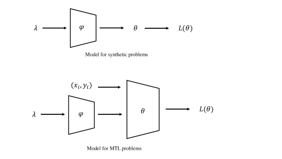
Figure 2: Model architecture of Pareto set models.

For PSL, we explain the function ${\bm{L}}({\bm{\theta}}_{\bm{\phi}}({\bm{\lambda}}))$ with more details as follows: In synthetic problems, the decision variable is directly the model output ${\bm{\theta}}_{\bm{\phi}}$, and ${\bm{\theta}}_{\bm{\phi}}$ is evaluated by the loss function. In multi-task learning (MTL) problems, ${\bm{\theta}}_{\bm{\phi}}({\bm{\lambda}})$ represents the parameters of a target network, and ${\bm{L}}({\bm{\theta}}_{\bm{\phi}}({\bm{\lambda}}))$ is evaluated using the dataset $({\bm{x}}_{i},{\bm{y}}_{i})$ with this target network. See Figure 2 for a visualization of these architectures.

The gradient of $\ell_{\mathrm{psl}}$ can be estimated by the chain rule:

$$\underbrace{\frac{\partial\ell_{\mathrm{psl}}}{\partial{\bm{\phi}}}}_{1\times D}=\mathbb{E}_{{\bm{\lambda}}\sim\mathrm{Unif}({\bm{\Delta}}_{m})}\underbrace{\frac{\partial\tilde{g}_{\bm{\lambda}}}{\partial{\bm{L}}}}_{{\bm{A}}:(1\times m)}\cdot\underbrace{\frac{\partial{\bm{L}}}{\partial{\bm{\theta}}}}_{{\bm{B}}:(m\times n)}\underbrace{\frac{\partial{\bm{\theta}}}{\partial{\bm{\phi}}}}_{{\bm{C}}:(n\times D)}.$$ (6)

The expectation is empirically estimated using a batch of $K$ preferences. The gradient vector ${\bm{A}}=(\tilde{\alpha}_{1},\ldots,\tilde{\alpha}_{m})$ is computed by the finite Pareto solution solver. The gradient matrix ${\bm{B}}$ can be calculated either via backpropagation (when gradients are easily obtained) or using a zero-order method. In Equation 6, ${\bm{C}}$ is always estimated through backpropagation, since ${\bm{\theta}}$ is a continuous vector function of ${\bm{\phi}}$. Gradient calculation by existing PSL methods is summarized in Table 4. After calculating the gradient of $\ell_{\mathrm{psl}}$, the parameter ${\bm{\phi}}$ is iteratively updated as ${\bm{\phi}}\xleftarrow{}{\bm{\phi}}-\eta\frac{\partial\ell_{\mathrm{psl}}}{\partial{\bm{\phi}}}$.

3.4 Multiobjective Bayesian optimization solvers

When the evaluation of objective functions is costly, multiobjective Bayesian optimization (MOBO) is often the preferred methodology for tackling such challenges. While there are several existing libraries, such as BoTorch [49] and HEBO [50], that facilities MOBO, they largely overlook algorithms that leverage decomposition techniques like PSL. To bridge this gap, LibMOON also includes three decomposition-based MOBO algorithms, including PSL-MOBO [26], PSL-DirHVEI [26, 51], and DirHV-EGO [51]. In each iteration, these methods build Gaussian process (GP) models for each objectives and generate a batch of query points for true function evaluations.

PSL-MOBO is an extension of PSL method for expensive MOPs. It optimizes the preference-conditional acquisition function $\alpha({\bm{\theta}}|{\bm{\lambda}})$ over an infinite number of preference vectors to generate a set of promising candidates:

$$\min_{\bm{\phi}}\ell_{\mathrm{psl}}=\mathbb{E}_{{\bm{\lambda}}\sim\mathrm{Unif}({\bm{\Delta}}_{m})}\left[\alpha({\bm{\theta}}_{\bm{\phi}}({\bm{\lambda}})|{\bm{\lambda}})\right],\qquad{\bm{\theta}}_{\bm{\phi}}({\bm{\lambda}}):{\bm{\Delta}}_{m}\xrightarrow{}\mathbb{R}^{N}.$$ (7)

Table 5: Supported preference-conditional acquisition functions. $p({\bm{y}}|{\bm{\theta}},\mathcal{D})=\mathcal{N}\left(\hat{{\bm{\mu}}}({\bm{\theta}}),\hat{\bm{\sigma}}^{2}({\bm{\theta}})\right)$ represents the posterior distribution over ${\bm{y}}={\bm{L}}({\bm{\theta}})$ obtained from GP models, $\beta$ is a parameter to balance exploration and exploitation, ${\bm{z}}^{*}=(z_{1}^{*},\ldots,z^{*}_{m})^{T}$ denotes a utopian point of the given MOP, and $\bm{\xi}=(\xi_{1},\ldots,\xi_{m})^{T}$ is a vector induced by the modified Tchebycheff scalarization.

	preference-conditional acquisition functions
Tch-LCB	$\alpha_{\mathrm{{TchLCB}}}({\bm{\theta}}|{\bm{\lambda}})=\underset{1\leq i\leq m}{\max}\{\lambda_{i}(\hat{\mu}_{i}({\bm{\theta}})-\beta\hat{\sigma}_{i}({\bm{\theta}})-z_{i}^{*})\}$
DirHV-EI	$\alpha_{\mathrm{{DirHVEI}}}({\bm{\theta}}|{\bm{\lambda}})=\mathbb{E}_{{\bm{y}}\sim p({\bm{y}}|{\bm{\theta}},\mathcal{D})}\left[\prod_{i=1}^{m}[\xi_{i}-y_{i}]_{+}\right]$

Currently, our library supports two representative preference-conditional acquisition functions: the Tchebycheff scalarization of lower confidence bound (Tch-LCB) [52, 26, 53] and the expected direction-based hypervolume improvement (DirHV-EI) [51]. We note that DirHV-EI can be regarded as an unbiased estimation of a weighted expected hypervolume improvement. Our library also supports DirHV-EGO, which employs a finite set of predetermined reference vectors as in [33].

4 Empirical studies

In this section, we study empirical results of LibMOON. Codes are basically run on a person computer with an i7-10700 CPU, and a 3080 GPU with 10G GPU memory. And we also conduct some analysis regarding to GPU ranging from 3080, 4060, and 4090. The empirical results contain five parts, MOO solvers for synthetic problems, Pareto set learning solvers for synthetic problems, MOO for MTL problems, Pareto set learning solvers for MTL problems, and GPU accelerations. The report of the first subsections .

4.1 MOO solvers for synthetic problems

We report the performance of various finite Pareto solution solvers using the VLMOP2 problem, formulated as follows:

$$\left\{\begin{aligned} \min_{{\bm{\theta}}}f_{1}({\bm{\theta}})&=1-\exp\left(-\sum_{i=1}^{n}\left(\theta_{i}-\frac{1}{\sqrt{n}}\right)^{2}\right),\\ \min_{{\bm{\theta}}}f_{2}({\bm{\theta}})&=1-\exp\left(-\sum_{i=1}^{n}\left(\theta_{i}+\frac{1}{\sqrt{n}}\right)^{2}\right).\end{aligned}\right.$$

This problem has been widely studied in the literature [14, 18] due to its PF has a non-convex shape . The visualization results are shown in Figure 3 and the numerical results are shown in Table 6.

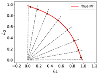
(a) Agg-COSMOS

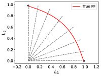
(b) Agg-LS

(c) Agg-PBI

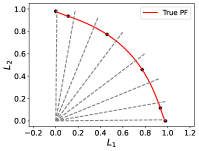
(d) Agg-SmoothTche

(e) Agg-Tche

(f) EPO

(g) HVGrad

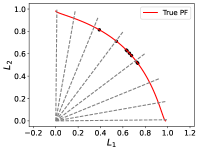
(h) MGDA-UB

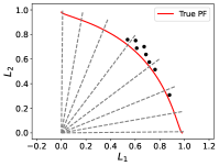
(i) MOO-SVGD

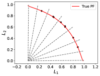
(j) PMTL

(k) Random

Figure 3: Finite Pareto solutions by different solvers on VLMOP2 problem.

Table 6: Numerical results of finite Pareto solutions for the VLMOP2 problem.

Method	Lmin	Smooth Lmin	Spacing	Sparsity	HV	IP	Cross Angle	PBI
EPO	0.162 (0.000)	0.061 (0.000)	0.029 (0.001)	0.043 (0.000)	0.283 (0.000)	0.776 (0.000)	0.046 (0.041)	0.930 (0.003)
MGDA-UB	0.012 (0.013)	-0.098 (0.011)	0.036 (0.011)	0.006 (0.001)	0.228 (0.008)	0.606 (0.010)	31.278 (1.533)	2.986 (0.088)
PMGDA	0.150 (0.001)	0.055 (0.000)	0.034 (0.001)	0.042 (0.000)	0.283 (0.000)	0.775 (0.000)	0.318 (0.037)	0.952 (0.003)
Random	0.000 (0.000)	-0.161 (0.002)	0.000 (0.000)	0.272 (0.000)	0.044 (0.000)	0.410 (0.127)	52.290 (12.938)	3.894 (0.590)
MOO-SVGD	0.060 (0.002)	-0.077 (0.004)	0.033 (0.018)	0.009 (0.003)	0.212 (0.003)	0.633 (0.024)	29.647 (3.305)	2.963 (0.197)
PMTL	0.014 (0.010)	-0.068 (0.009)	0.061 (0.020)	0.018 (0.007)	0.260 (0.012)	0.706 (0.004)	15.036 (1.270)	1.993 (0.093)
HVGrad	0.182 (0.000)	0.067 (0.000)	0.016 (0.000)	0.041 (0.000)	0.286 (0.000)	0.578 (0.069)	34.090 (8.607)	3.062 (0.465)
Agg-LS	0.000 (0.000)	-0.159 (0.001)	0.002 (0.001)	0.272 (0.001)	0.043 (0.002)	0.227 (0.008)	71.168 (0.958)	4.764 (0.047)
Agg-Tche	0.158 (0.001)	0.061 (0.000)	0.031 (0.001)	0.043 (0.000)	0.283 (0.000)	0.348 (0.000)	55.174 (0.049)	3.889 (0.004)
Agg-PBI	0.113 (0.074)	0.032 (0.046)	0.045 (0.030)	0.042 (0.002)	0.281 (0.002)	0.657 (0.097)	11.374 (9.125)	1.434 (0.402)
Agg-COSMOS	0.141 (0.000)	0.045 (0.000)	0.035 (0.000)	0.039 (0.000)	0.285 (0.000)	0.771 (0.000)	1.085 (0.000)	1.011 (0.000)
Agg-SmoothTche	0.004 (0.000)	-0.074 (0.000)	0.154 (0.001)	0.074 (0.000)	0.244 (0.000)	0.276 (0.000)	63.106 (0.018)	4.253 (0.001)

• All methods were run five times with random seeds, presented as (mean)(std).

We present the following key findings:

1. Agg-COSMOS produces approximate ‘exact’ Pareto solutions (the corresponding Pareto objectives aligned with preference vectors). This is due to a cosine similarity term in Agg-COSMOS encouraging the Pareto objectives be close to preference vectors.

2. Agg-LS can only find two endpoints on this problem since PF of VLMOP2 is of non-convex shape. Different preference vectors correspond to duplicated Pareto solutions.

3. Agg-PBI generates “exact” Pareto solutions when the coefficient of $d_{2}$ exceeds a specific value, as guaranteed by PBI [54]. However, this parameter is challenging to tune and is influenced by the Pareto front’s curvature. Additionally, PBI can transform a convex multi-objective optimization problem into a non-convex one, making Agg-PBI less recommended.

4. Agg-Tche generates diverse solutions and produces exact Pareto solutions corresponding to the inverse of the preference vector. Both Agg-Tche and Agg-SmoothTche retain the convexity of objectives, meaning their aggregation functions remain convex when all objectives are convex. However, the solution distribution of Agg-SmoothTche cannot be precisely determined due to the involvement of a temperature coefficient $h$.

5. HVGrad updates the decision variable using the hypervolume gradient, resulting in the largest hypervolume. PMTL, a two-stage method, can struggle with tuning warm-up iterations, leading to poor initialization and less diverse solutions. MOO-SVGD’s update direction has two conflicting goals: promoting diversity and ensuring convergence. This conflict makes MOO-SVGD difficult to converge, often requiring 10 times more iterations than other methods, resulting in poor convergence behavior.

6. Among the methods, MGDA-UB, Random, Agg-PBI, and MOO-SVGD exhibit relatively large deviations. MGDA-UB and Random generate arbitrary Pareto solutions due to their computation nature. Agg-PBI results in non-convex aggregation functions, leading to variable solutions based on different random initializations. MOO-SVGD has high standard deviation because its optimization process is unstable, and its balance between convergence and diversity is unclear.

4.2 Pareto set learning on synthetic problems

In this section, we present PSL results using the synthetic VLMOP2 problem as an example. Visualizations of the predicted Pareto solutions are shown in Figure 4, and numerical results are reported in Table 7. From the table and figure, we have the following key findings:

Table 7: Pareto set learning results on VLMOP2 problem.

Method	Lmin	Smooth Lmin	Spacing	Sparsity	HV	IP	Cross Angle	PBI	Span
Agg-COSMOS	0.045 (0.000)	-0.127 (0.000)	1.560 (0.004)	0.525 (0.000)	0.318 (0.000)	0.752 (0.000)	0.950 (0.001)	0.995 (0.000)	0.907 (0.000)
Agg-LS	0.000 (0.000)	-0.258 (0.000)	0.115 (0.094)	13.245 (1.871)	0.045 (0.003)	0.239 (0.001)	70.541 (0.156)	4.811 (0.007)	0.982 (0.000)
Agg-Tche	0.047 (0.004)	-0.121 (0.000)	1.476 (0.146)	0.579 (0.008)	0.319 (0.000)	0.383 (0.003)	51.558 (0.280)	3.775 (0.011)	0.955 (0.005)
Agg-SmoothTche	0.000 (0.000)	-0.187 (0.000)	6.711 (0.003)	1.060 (0.000)	0.302 (0.000)	0.300 (0.000)	60.386 (0.001)	4.169 (0.000)	0.982 (0.000)
EPO	0.050 (0.001)	-0.120 (0.000)	1.332 (0.078)	0.583 (0.005)	0.319 (0.000)	0.756 (0.000)	0.388 (0.098)	0.952 (0.008)	0.961 (0.003)
PMGDA	0.047 (0.000)	-0.121 (0.000)	1.446 (0.051)	0.580 (0.002)	0.319 (0.000)	0.756 (0.000)	0.215 (0.062)	0.939 (0.005)	0.958 (0.001)

1. PSL with the COSMOS aggregation function fails to find all marginal Pareto solutions because COSMOS does not guarantee the discovery of the entire Pareto set/front. PSL with linear scalarization function could not fit the two endpoints of the PF.

2. PSL with the smooth Tchebycheff function finds diverse Pareto solutions due to the unclear relationship between preference vectors and Pareto objectives. PSL using Tche., EPO, and PMGDA as base solvers can discover the entire PS/PF, as all three methods effectively find exact Pareto solutions. By traversing the entire preference space, the Pareto model fits the entire Pareto set accurately.

(a) Agg-COSMOS

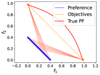
(b) Agg-LS

(c) Agg-SmoothTche

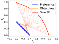
(d) Agg-Tche

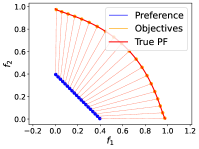
(e) EPO

(f) PMGDA

Figure 4: Predicted Pareto solutions by different PSL solvers on VLMOP2 problem.

4.3 MOO solvers for MTL problems

In this section, we investigate the performance of different finite Pareto solution solvers on the Adult dataset, which is a multitask learning task called fairness classification. For this task, the decision variable $\theta$ is the parameter of a fully-connected neural network, with $|{\bm{\theta}}|=28033$. The first objective function is the cross entropy loss, and the second objective is the hyperbolic tangent relaxation of the difference of equality of opportunity (DEO) loss [37][Eq. 6]. The visualization on the Adult problem is shown in Figure 5 and the numerical result is shown in Table 8.

From the table and figure, we have the following key findings:

1. Agg-LS has two main drawbacks: it cannot identify the non-convex parts of the Pareto front (as previously mentioned), and the relationship between preference vectors and Pareto objectives is unknown, making it challenging to select appropriate preference vectors. Agg-PBI and Agg-COSMOS only find a small portion of the PF due to it is hard to set the coefficients.

2. Agg-SmoothmTche and Agg-mTche perform well on this task, as they can accurately find Pareto solutions. Once the Pareto front range is known, diverse solutions can be easily found using uniform preference vectors.

3. The Random method and MGDA-UB only find a single Pareto solution, since the position of this solution cannot be controlled by these methods.

4. Among the three methods that directly find a set of Pareto solutions (MOO-SVGD, PMTL, and HV-Grad), HV-Grad produces the most diverse solutions with the largest hypervolume. PMTL, being a two-stage method, can encounter issues when solutions fall outside the sector due to stochastic factors. MOO-SVGD optimizes both convergence and diversity but is generally unstable based on our tests.

(a) Agg-COSMOS

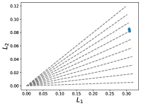
(b) Agg-LS

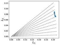
(c) Agg-PBI

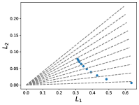
(d) Agg-SmoothmTche

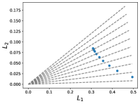
(e) Agg-mTche

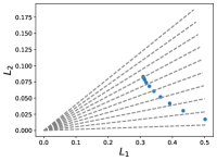
(f) EPO

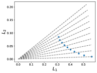
(g) HVGrad

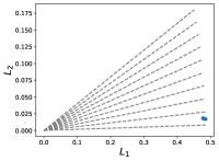
(h) MGDA-UB

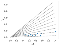
(i) MOO-SVGD

(j) PMTL

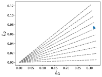
(k) Random

Figure 5: Finite Pareto solutions by different solvers on Adult problem.

Table 8: Numerical results of finite Pareto solutions for the Adult problem.

Method	Lmin	Smooth Lmin	Spacing	Sparsity	HV	IP	Cross Angle	PBI	Span
Agg-COSMOS	0.004 (0.000)	-0.194 (0.000)	0.463 (0.004)	0.014 (0.001)	0.657 (0.000)	0.295 (0.000)	2.787 (0.013)	0.426 (0.000)	0.052 (0.000)
Agg-LS	0.000 (0.000)	-0.223 (0.000)	0.016 (0.005)	0.000 (0.000)	0.636 (0.001)	0.272 (0.001)	6.595 (0.028)	0.500 (0.001)	0.002 (0.000)
Agg-PBI	0.001 (0.000)	-0.216 (0.000)	0.107 (0.008)	0.001 (0.000)	0.642 (0.000)	0.277 (0.001)	4.995 (0.007)	0.462 (0.001)	0.010 (0.000)
Agg-SmoothmTche	0.005 (0.001)	-0.163 (0.000)	4.237 (0.029)	0.329 (0.003)	0.675 (0.001)	0.347 (0.001)	3.385 (0.053)	0.500 (0.002)	0.072 (0.000)
Agg-mTche	0.002 (0.000)	-0.177 (0.000)	2.034 (0.072)	0.091 (0.004)	0.674 (0.000)	0.316 (0.000)	1.962 (0.045)	0.422 (0.001)	0.067 (0.001)
EPO	0.002 (0.000)	-0.175 (0.000)	2.136 (0.054)	0.101 (0.004)	0.674 (0.001)	0.320 (0.000)	2.002 (0.025)	0.426 (0.001)	0.066 (0.000)
MGDA-UB	0.000 (0.000)	-0.222 (0.001)	0.050 (0.039)	0.000 (0.000)	0.510 (0.003)	0.410 (0.004)	9.586 (0.072)	0.878 (0.011)	0.001 (0.000)
Random	0.000 (0.000)	-0.224 (0.000)	0.040 (0.016)	0.000 (0.000)	0.633 (0.001)	0.279 (0.000)	5.863 (0.010)	0.491 (0.000)	0.002 (0.000)
PMTL	0.002 (0.001)	-0.176 (0.002)	2.236 (0.045)	0.156 (0.028)	0.617 (0.002)	0.372 (0.004)	7.039 (0.242)	0.675 (0.016)	0.035 (0.001)
MOO-SVGD	0.049 (0.007)	-0.079 (0.003)	5.382 (4.539)	2.660 (1.857)	0.548 (0.005)	0.657 (0.013)	8.354 (0.211)	1.274 (0.029)	0.065 (0.010)
HVGrad	0.014 (0.002)	-0.153 (0.002)	1.347 (0.041)	0.110 (0.003)	0.678 (0.001)	0.347 (0.004)	7.043 (0.260)	0.663 (0.017)	0.075 (0.001)

• All methods were run five times with random seeds, presented as (mean)(std).

4.4 Pareto set learning on MTL

This section presents the Pareto set learning results on the MO-MNIST problem using a hypernet architecture. The model was trained for 20 epochs, optimizing approximately 3.24M parameters, with the first and second objectives being the cross-entropy losses for the top-right and bottom-left images. EPO-based PSL and PMGDA-based PSL are not very suitable for this task since manipulating gradient of 3.2M dim is not efficient, the visualization results are reported in Figure 6 and numerical results in Table 9.

From the table and figure, we have the following key findings:

1. The Pareto Front (PF) of this task is nearly convex, indicating that Linear scalarazation (LS) can efficiently find the entire Pareto front. Therefore, it is not necessary to employ complex Multi-Objective Optimization (MOO) methods.

2. Agg-LS significantly outperforms other methods on this task, as evidenced by the substantially higher Hypervolume (HV). Furthermore, the training losses across other methods show minimal reduction, indicating that for this challenging task, the convergence of other non-linear scalarization methods is extremely slow.

3. Agg-SmoothTche and Agg-Tche produce duplicate marginal Pareto solutions because selecting appropriate weight factors is challenging.

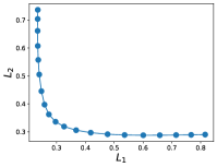
(a) Agg-COSMOS

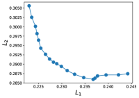
(b) Agg-LS

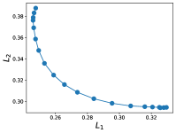
(c) Agg-SmoothTche

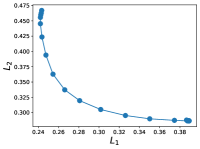
(d) Agg-Tche

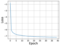
(e) Agg-COSMOS

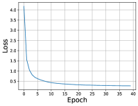
(f) Agg-LS

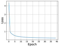
(g) Agg-SmoothTche

(h) Agg-Tche

Figure 6: Training process for generating predicted Pareto solutions using different PSL solvers on MO-MNIST problem.

Table 9: Pareto set learning results on MO-MNITS problem.

Method	Lmin	Smooth Lmin	Spacing	Sparsity	HV	IP	Cross Angle	PBI	Span
Agg-COSMOS	0.033 (0.002)	-0.152 (0.007)	0.967 (0.202)	0.278 (0.038)	0.512 (0.015)	0.535 (0.028)	9.208 (0.541)	1.221 (0.050)	0.497 (0.043)
Agg-LS	0.001 (0.000)	-0.286 (0.002)	0.068 (0.029)	0.000 (0.000)	0.557 (0.004)	0.257 (0.004)	27.536 (0.116)	1.149 (0.021)	0.016 (0.003)
Agg-PBI	0.000 (0.000)	-0.295 (0.000)	0.019 (0.006)	0.000 (0.000)	0.536 (0.008)	0.269 (0.005)	26.270 (0.117)	1.150 (0.019)	0.002 (0.001)
Agg-SmoothTche	0.001 (0.000)	-0.248 (0.002)	0.440 (0.040)	0.012 (0.001)	0.538 (0.008)	0.281 (0.005)	32.244 (0.417)	1.471 (0.007)	0.087 (0.012)
Agg-Tche	0.000 (0.000)	-0.235 (0.004)	0.988 (0.110)	0.045 (0.015)	0.533 (0.010)	0.292 (0.008)	35.292 (0.742)	1.693 (0.075)	0.131 (0.014)

4.5 MOBO for synthetic and real-world problems

In this section, we test three MOBO algorithms in LibMOON on three benchmark problems, including ZDT1, RE21, VLMOP1 and VLMOP2. To ensure a fair comparison, we generate $11n-1$ initial samples using Latin Hypercube Sampling for each method. The maximum number of function evaluations is set as 200. Our experimental results, illustrated in Figure 4, clearly demonstrate the rapid convergence capabilities of all three methods. DirHV-EGO, PSL-DirHV-EI, and PSL-MOBO not only efficiently navigate the solution space but also quickly reach optimal solutions. This highlights the robustness and effectiveness of our implemented algorithms in handling different types of MOPs.

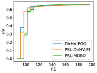
(a) ZDT1

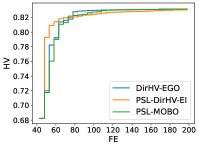
(b) RE21

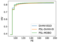
(c) VLMOP1

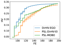
(d) VLMOP2

Figure 7: HV curves on MOBO problem. Results are averaged on five random seeds. Reference point to calculate HV : [1.2,1.2].

4.6 GPU acceleration

We evaluate LibMOON performance on Pareto set learning for the MO-MNIST problem across various platforms (CPU, RTX 3080, 4060, 4090). Running times are detailed in Table 10 and visualized in Figure 8. The table and figure show a significant reduction in time (about one-third) when using a personal GPU compared to a CPU. The RTX 4090 further reduces time by approximately 25% compared to the RTX 4060.

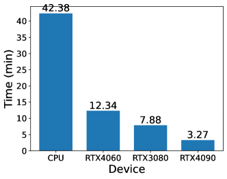
Figure 8: Running time for Pareto set learning on the MO-MNIST problem using different devices using 3M parameters.

Table 10: Running time (minutes) for different platforms on the MO-MNIST problem.

Platform	MO-MNIST	MO-Fashion	Fashion-MNIST
CPU	43.43	44.45	46.45
RTX 4060 (8G)	14.72	13.21	12.43
RTX 3080 (10G)	7.88	7.16	7.17
RTX 4090 (24G)	3.27	3.27	3.27

• We run all datasets for 100 epochs using 3M parameters on a 13th Gen Intel(R) Core(TM) i9-13900HX CPU.

5 Conclusion, limitations, and further works

Conclusion.

We introduced the first gradient-based multiobjective optimization framework called LibMOON, which is implemented based on the PyTorch environment for the research community’s convenience. LibMOON supports mainstream gradient-based MOO methods; the modular design of LibMOON further allows the library to address various MOPs, including discrete Pareto solution optimization, Pareto set learning, multiobjective Bayesian optimization, etc., in a plug-and-play manner. LibMOON can thus be leveraged to quickly yet robustly test new MOO ideas.

Limitations.

The limitations of LibMOON include: (1) the rapid development of gradient-based MOO methods makes it impossible to incorporate all relevant techniques, so some effective methods may be missing; (2) the codebase, primarily based on works from Prof. Qingfu Zhang’s group, may not easily accommodate new methods.

Future Work.

Future work includes: (1) maintaining a user and development community to address issues promptly, and (2) adding newly published or well-known methods to the library as quickly as possible.

Appendix A Appendix

A.1 Full name and notation tables

This section lists the full names of optimization methods and terms for clarity (Table 11) and provides notation in Table 12.

A.2 Aggregation functions

Aggregation function convert an MOP into a single-objective optimization problem under a specific preference vector ${\bm{\lambda}}$. Some popular aggregation functions are:

1. COSMOS:

   $$g^{\mathrm{cosmos}}_{\bm{\lambda}}({\bm{\theta}})={\bm{\lambda}}^{\top}{\bm{L}}({\bm{\theta}})-\mu\frac{{\bm{\lambda}}^{\top}{\bm{L}}({\bm{\theta}})}{\|{\bm{\lambda}}\|\|{\bm{L}}({\bm{\theta}})\|},$$ (8)

   where $\mu$ is a positive weight factor to align the objective vector ${\bm{L}}({\bm{\theta}})$ with the preference vector ${\bm{\lambda}}$.

2. Linear scalarization (LS):

   $$g^{\mathrm{LS}}_{\bm{\lambda}}({\bm{\theta}})=\sum_{i=1}^{m}\lambda_{i}L_{i}({\bm{\theta}}).$$ (9)

3. Tchebycheff (Tche):

   $$g^{\mathrm{Tche}}_{\bm{\lambda}}({\bm{\theta}})=\max_{1\leq i\leq m}\left\{\lambda_{i}(L_{i}({\bm{\theta}})-z_{i})\right\},$$ (10)

   where ${\bm{z}}$ is a reference point, usually set as the nadir point the minimal value in each objectives.

4. Modified Tchebycheff (mTche):

   $$g^{\mathrm{mTche}}_{\bm{\lambda}}({\bm{\theta}})=\max_{1\leq i\leq m}\left\{\frac{L_{i}({\bm{\theta}})-z_{i}}{\lambda_{i}}\right\},$$ (11)

   where ${\bm{z}}$ is a reference point, the same as the point used in the Tchebycheff scalarization function.

5. Smooth Tchebycheff (STche):

   $$g^{\mathrm{STche}}_{\bm{\lambda}}({\bm{\theta}})=\frac{1}{h}\log\left(\sum_{i=1}^{m}\exp(h\cdot\lambda_{i}(L_{i}({\bm{\theta}})-z_{i}))\right).$$ (12)

   The Smooth Tchebycheff function uses a relaxed Smooth $\max$ operator. The advantage of this approach is that $g^{\mathrm{STche}}_{\bm{\lambda}}({\bm{\theta}})$ becomes a Smooth function if each objective function $L_{i}({\bm{\theta}})$ is Smooth, unlike the non-Smooth $g^{\mathrm{Tche}}_{\bm{\lambda}}({\bm{\theta}})$. Smooth functions generally have faster convergence compared to non-Smooth ones. Similarly, we can define the Smooth modified Tchebycheff function.

6. Penalty-Based Intersection (PBI):

   $$g^{\mathrm{PBI}}_{\bm{\lambda}}({\bm{\theta}})=\underbrace{\frac{1}{\left\lVert{\bm{\lambda}}\right\rVert}\cdot\sum_{i=1}^{m}\lambda_{i}L_{i}({\bm{\theta}})}_{d_{1}}+\mu\underbrace{\left\lVert{\bm{L}}({\bm{\theta}})-\frac{d_{1}}{\left\lVert{\bm{\lambda}}\right\rVert}\cdot{\bm{\lambda}}\right\rVert}_{d_{2}},$$ (13)

   where $\mu$ is a positive weight factor that encourage a objective to align with a preference vector ${\bm{\lambda}}$.

7. $p$-norm:

   $$g^{\mathrm{pnorm}}_{\bm{\lambda}}({\bm{\theta}})=\sqrt[\frac{1}{p}]{\left\lVert{\bm{\lambda}}\odot{\bm{L}}({\bm{\theta}})-{\bm{z}}\right\rVert_{p}}.$$ (14)

   The symbol $\odot$ denotes the element-wise product between two vectors.

8. Augmented Achievement Scalarization Function (AASF):

   $$g^{\mathrm{AASF}}_{\bm{\lambda}}({\bm{\theta}})=g^{\mathrm{mTche}}_{\bm{\lambda}}({\bm{\theta}})+\rho g^{\mathrm{LS}}_{\bm{\lambda}}({\bm{\theta}}),$$ (15)

   where $\rho$ is small positive coefficient, usually set as 0.1.

   The contour curve for this functions for a bi-objective case can be found in https://libmoondocs.readthedocs.io/en/latest/gallery/aggfuns.html.

Table 11: Short name to full name table

Short Name	Full name
MOP	Multiobjective Optimization Problem
SOP	Singleobjective Optimization Problem
MOO	MultiObjective Optimization
MOEA	MultiObjective Evolutionary Algorithm
MOBO	MultiObjective Baysian Optimization
PSL	Pareto Set Learning
PS	Pareto Set
PF	Pareto Front
‘exact’ Pareto solution	The corresponding Pareto objective aligns with a given preference vector
ES	Evolutionary strategy
BP	Backward propagation
PMTL [18]	Pareto Multa-Task Learning
MOO-SVGD [19]	MultiObjective Optimization Stein Variational Gradient Descent
EPO [14]	Exact Pareto Optimization
PMGDA [40]	Preference based Multiple Gradient Descent Algorithm
Agg-LS [42]	Aggregation function with Linear Scalarization
Agg-PBI [33]	Aggregation function with Penalty Based Intersection
Agg-Tche [33]	Aggregation function with Tchebycheff scalarization
Agg-mTche [43]	Aggregation function with modified Tchebycheff scalarization
Agg-COSMOS [37]	Aggregation function with COSMOS scalarization
RE problems	Realworld problems

Table 12: Notations used in this paper

Notation	Meaning
${\bm{\theta}}$	The decision variable of an MOP.
${\bm{\phi}}$	The decision variable of a Pareto set model.
$m$	Number of objectives.
$n$	Number of decision variables.
$K$	Number of finite Pareto solutions.
$\alpha_{i}$	Coefficients of objective functions.
${\bm{\lambda}}$	A preference vector.

A.3 Metrics

Metrics can be categorized into two groups. The first group evaluates the quality of a set of solutions ${\mathbb{Y}}=\{{\bm{y}}^{(1)},\ldots,{\bm{y}}^{(N)}\}$, with specific metrics such as IGD and FD relying on the known Pareto front for accuracy.

The second group of metrics assesses the quality of individual solutions ${\bm{y}}$ when a preference vector ${\bm{\lambda}}$ is provided.

Group 1: Metrics for a set of solutions

1. Hypervolume (HV) ($\uparrow$) [55]: This metric evaluates both the convergence to the Pareto Front (PF) and the diversity of solutions. A low HV value indicates poor convergence, while high HV values imply better performance. The hypervolume is calculated as the volume dominated by at least one solution in the set ${\mathbb{S}}$ with respect to a reference point ${\bm{r}}$:

   $$\mathrm{HV}_{\bm{r}}({\mathbb{S}})=\mathrm{Vol}({{\bm{y}}\;|\;\exists{\bm{y}}^{\prime}\in{\mathbb{S}},{\bm{y}}^{\prime}\preceq{\bm{y}}\preceq{\bm{r}}}).$$

2. Inverted Generational Distance (IGD) [56]: IGD measures the average distance between points in a reference set ${\mathbb{Z}}$ and the nearest solutions in the set ${\mathbb{S}}$:

   $$\operatorname{IGD}({\mathbb{S}})=\frac{1}{|{\mathbb{Z}}|}\left(\sum_{i=1}^{|{\mathbb{Z}}|}\min_{{\bm{y}}^{\prime}\in{\mathbb{S}}}\rho({\bm{y}}^{(i)},{\bm{y}}^{\prime})^{2}\right)^{1/2}.$$

3. Fill Distance (FD) [57]: This metric calculates the covering radius of a set of solutions ${\mathbb{S}}$, defined as the maximum minimum distance from any point in the reference set ${\mathbb{Z}}$ to the nearest solution in ${\mathbb{Z}}$:

   $$\mathrm{FD}({\mathbb{S}})=\max_{{\bm{y}}^{\prime}\in{\mathbb{Z}}}\min_{{\bm{y}}\in{\mathbb{S}}}\rho({\bm{y}},{\bm{y}}^{\prime}).$$ (16)

4. Minimal Distance ($\mathrm{l}_{\min}$): This metric captures the smallest pairwise distance among all objectives:

   $$\mathrm{l}_{\min}=\min_{1\leq i<j\leq N}\rho({\bm{y}}^{(i)},{\bm{y}}^{(j)})$$

   where $\rho()$ denotes the Euclidean distance.

5. Smooth Minimal Distance ($\mathrm{sl}_{\min}$): This metric is a “smooth-min" version of the minimal distance function, defined as:

   $$\mathrm{sl}_{\min}=-\frac{1}{h\cdot k(k-1)}\log\left(\sum_{1\leq i<j\leq N}\exp\left(-h\rho\left({\bm{y}}^{(i)},{\bm{y}}^{(j)}\right)\right)\right).$$ (17)

6. Spacing: This metric measures the standard deviation of the minimal distances from one solution to others, with lower values indicating a more uniform distribution of objective vectors:

   $$\mathrm{spacing}=\frac{1}{N}\sum_{i=1}^{N}(d_{i}-\bar{d})^{2},\qquad\bar{d}=\frac{1}{N}\sum_{i=1}^{N}d_{i},\qquad d_{i}=\min_{1\leq i\neq j\leq N}\rho({\bm{y}}^{(i)},{\bm{y}}^{(j)}).$$ (18)

7. Span: This metric evaluates the range (span) of solutions in their minimal dimension, defined as:

   $$\mathrm{Span}=\min_{1\leq i\leq m}\max_{1\leq k<l\leq N}|y_{i}^{(k)}-y_{i}^{(l)}|.$$ (19)

Group 2: Metrics for individual solutions

1. Penalty-based Intersection (PBI): This metric is a weighted sum of two distance functions $d_{1}$ and $d_{2}$, given by $\mathrm{PBI}=d_{1}+\mu d_{2}$, where

   $$d_{1}=\frac{\langle{\bm{y}}-{\bm{z}},{\bm{\lambda}}\rangle}{\left\lVert{\bm{\lambda}}\right\rVert},\qquad d_{2}=\left\lVert{\bm{y}}-(d_{1}{\bm{\lambda}}+{\bm{z}})\right\rVert.$$ (20)

2. Inner Product (IP): This metric measures the alignment of the objective vector ${\bm{y}}$ with the preference vector ${\bm{\lambda}}$:

   $$\mathrm{IP}=\langle{\bm{y}},{\bm{\lambda}}\rangle.$$ (21)

3. Cross Angle ($\vartheta$): For bi-objective problems, this metric measures the angular difference between the objective vector and the preference vector:

   $$\vartheta=\left\lVert\arctan(y_{2}/y_{1})-\arctan(\lambda_{2}/\lambda_{1})\right\rVert.$$ (22)

Those metrics are summarized in Table 13 and also can be found in https://libmoondocs.readthedocs.io/en/latest/apis/Libmoon_metric.html.

Table 13: Supported metrics.

Metrics	Full name	Descriptions
HV	Hypervolume	Hypervolume value of the dominated region.
IGD	Inverted general distance	The average general distance between a set and the true PF.
FD	Fill distance	The radius of a set to cover the true PF.
$\mathrm{l}_{\min}$	Minimal distance	The minimal pairwise distance of a set.
$\mathrm{sl}_{\min}$	Smooth minimal distance	The smooth minimal pairwise distance of a set.
Spacing	-	The standard deviation of the minimal distances to other solutions.
Span	-	The range of a set.
PBI	Penalty-based intersection	The weighted distance between inner product and distance to a preference vector.
IP	Inner product	The inner product between a preference and an objective vector.
$\vartheta$	Cross product	The cross angle between a preference and an objective vector.

A.4 License and usage of LibMOON

The license used for Adult/Compas/Credit follows Creative Commons Attribution 4.0 International (CC BY 4.0), Database Contents License (DbCL) v1.0, and CC0: Public Domain, respectively. For academic use of LibMOON, please cite our paper or GitHub. Commercial use requires author permission.

References

- [1] Han Zhao and Geoffrey J Gordon. Inherent tradeoffs in learning fair representations. The Journal of Machine Learning Research, 23(1):2527–2552, 2022.
- [2] Ruicheng Xian, Lang Yin, and Han Zhao. Fair and optimal classification via post-processing. In International Conference on Machine Learning, pages 37977–38012. PMLR, 2023.
- [3] Martim Brandao, Maurice Fallon, and Ioannis Havoutis. Multi-controller multi-objective locomotion planning for legged robots. In 2019 IEEE/RSJ international conference on intelligent robots and systems (IROS), pages 4714–4721. IEEE, 2019.
- [4] Jie Xu, Yunsheng Tian, Pingchuan Ma, Daniela Rus, Shinjiro Sueda, and Wojciech Matusik. Prediction-guided multi-objective reinforcement learning for continuous robot control. In International conference on machine learning, pages 10607–10616. PMLR, 2020.
- [5] Dietmar Jannach. Multi-objective recommender systems: Survey and challenges. arXiv preprint arXiv:2210.10309, 2022.
- [6] Ee Yeo Keat, Nurfadhlina Mohd Sharef, Razali Yaakob, Khairul Azhar Kasmiran, Erzam Marlisah, Norwati Mustapha, and Maslina Zolkepli. Multiobjective deep reinforcement learning for recommendation systems. IEEE Access, 10:65011–65027, 2022.
- [7] Fatima Ezzahra Zaizi, Sara Qassimi, and Said Rakrak. Multi-objective optimization with recommender systems: A systematic review. Information Systems, 117:102233, 2023.
- [8] Matthias Ehrgott. Multicriteria optimization, volume 491. Springer Science & Business Media, 2005.
- [9] Ye Tian, Ran Cheng, Xingyi Zhang, and Yaochu Jin. Platemo: A matlab platform for evolutionary multi-objective optimization [educational forum]. IEEE Computational Intelligence Magazine, 12(4):73–87, 2017.
- [10] Francesco Biscani and Dario Izzo. A parallel global multiobjective framework for optimization: pagmo. Journal of Open Source Software, 5(53):2338, 2020.
- [11] Julian Blank, Kalyanmoy Deb, Yashesh Dhebar, Sunith Bandaru, and Haitham Seada. Generating well-spaced points on a unit simplex for evolutionary many-objective optimization. IEEE Transactions on Evolutionary Computation, 25(1):48–60, 2020.
- [12] Panagiotis Kyriakis and Jyotirmoy Deshmukh. Pareto policy adaptation. In International Conference on Learning Representations, volume 2022, 2022.
- [13] Ozan Sener and Vladlen Koltun. Multi-task learning as multi-objective optimization. Advances in neural information processing systems, 31, 2018.
- [14] Debabrata Mahapatra and Vaibhav Rajan. Multi-task learning with user preferences: Gradient descent with controlled ascent in pareto optimization. In International Conference on Machine Learning, pages 6597–6607. PMLR, 2020.
- [15] Xi Lin, Zhiyuan Yang, Qingfu Zhang, and Sam Kwong. Controllable pareto multi-task learning. arXiv preprint arXiv:2010.06313, 2020.
- [16] Aviv Navon, Aviv Shamsian, Gal Chechik, and Ethan Fetaya. Learning the pareto front with hypernetworks. arXiv preprint arXiv:2010.04104, 2020.
- [17] Kalyanmoy Deb, Aryan Gondkar, and Suresh Anirudh. Learning to predict pareto-optimal solutions from pseudo-weights. In International Conference on Evolutionary Multi-Criterion Optimization, pages 191–204. Springer, 2023.
- [18] Xi Lin, Hui-Ling Zhen, Zhenhua Li, Qing-Fu Zhang, and Sam Kwong. Pareto multi-task learning. Advances in neural information processing systems, 32, 2019.
- [19] Xingchao Liu, Xin Tong, and Qiang Liu. Profiling pareto front with multi-objective stein variational gradient descent. Advances in Neural Information Processing Systems, 34:14721–14733, 2021.
- [20] Yuzheng Hu, Ruicheng Xian, Qilong Wu, Qiuling Fan, Lang Yin, and Han Zhao. Revisiting scalarization in multi-task learning: A theoretical perspective. arXiv preprint arXiv:2308.13985, 2023.
- [21] Sebastian Peitz and Michael Dellnitz. Gradient-based multiobjective optimization with uncertainties. In NEO 2016: Results of the Numerical and Evolutionary Optimization Workshop NEO 2016 and the NEO Cities 2016 Workshop held on September 20-24, 2016 in Tlalnepantla, Mexico, pages 159–182. Springer, 2018.
- [22] Sagar Imambi, Kolla Bhanu Prakash, and GR Kanagachidambaresan. Pytorch. Programming with TensorFlow: Solution for Edge Computing Applications, pages 87–104, 2021.
- [23] Stephen P Boyd and Lieven Vandenberghe. Convex optimization. Cambridge university press, 2004.
- [24] Yifan Zhong, Chengdong Ma, Xiaoyuan Zhang, Ziran Yang, Qingfu Zhang, Siyuan Qi, and Yaodong Yang. Panacea: Pareto alignment via preference adaptation for llms. arXiv preprint arXiv:2402.02030, 2024.
- [25] Xi Lin, Xiaoyuan Zhang, Zhiyuan Yang, Fei Liu, Zhenkun Wang, and Qingfu Zhang. Smooth tchebycheff scalarization for multi-objective optimization. In International conference on machine learning. PMLR, 2024.
- [26] Xi Lin, Zhiyuan Yang, Xiaoyuan Zhang, and Qingfu Zhang. Pareto set learning for expensive multi-objective optimization. Advances in Neural Information Processing Systems, 35:19231–19247, 2022.
- [27] Baijiong Lin and Yu Zhang. Libmtl: A python library for deep multi-task learning. The Journal of Machine Learning Research, 24(1):9999–10005, 2023.
- [28] Juan J. Durillo, Antonio J. Nebro, and Enrique Alba. The jmetal framework for multi-objective optimization: Design and architecture. In IEEE Congress on Evolutionary Computation, pages 1–8, 2010.
- [29] J. Blank and K. Deb. pymoo: Multi-objective optimization in python. IEEE Access, 8:89497–89509, 2020.
- [30] Kalyanmoy Deb, Amrit Pratap, Sameer Agarwal, and TAMT Meyarivan. A fast and elitist multiobjective genetic algorithm: Nsga-ii. IEEE transactions on evolutionary computation, 6(2):182–197, 2002.
- [31] Kalyanmoy Deb and Himanshu Jain. An evolutionary many-objective optimization algorithm using reference-point-based nondominated sorting approach, part i: Solving problems with box constraints. IEEE Transactions on Evolutionary Computation, 18(4):577–601, 2014.
- [32] Himanshu Jain and Kalyanmoy Deb. An evolutionary many-objective optimization algorithm using reference-point based nondominated sorting approach, part ii: Handling constraints and extending to an adaptive approach. IEEE Transactions on Evolutionary Computation, 18(4):602–622, 2014.
- [33] Qingfu Zhang and Hui Li. Moea/d: A multiobjective evolutionary algorithm based on decomposition. IEEE Transactions on evolutionary computation, 11(6):712–731, 2007.
- [34] Nicola Beume, Boris Naujoks, and Michael Emmerich. Sms-emoa: Multiobjective selection based on dominated hypervolume. European Journal of Operational Research, 181(3):1653–1669, 2007.
- [35] Nihat Engin Toklu, Timothy Atkinson, Vojtěch Micka, Paweł Liskowski, and Rupesh Kumar Srivastava. Evotorch: Scalable evolutionary computation in python. arXiv preprint arXiv:2302.12600, 2023.
- [36] Beichen Huang, Ran Cheng, Zhuozhao Li, Yaochu Jin, and Kay Chen Tan. Evox: A distributed gpu-accelerated framework for scalable evolutionary computation. IEEE Transactions on Evolutionary Computation, 2024.
- [37] Michael Ruchte and Josif Grabocka. Scalable pareto front approximation for deep multi-objective learning. In 2021 IEEE international conference on data mining (ICDM), pages 1306–1311. IEEE, 2021.
- [38] Kirtan Padh, Diego Antognini, Emma Lejal-Glaude, Boi Faltings, and Claudiu Musat. Addressing fairness in classification with a model-agnostic multi-objective algorithm. In Uncertainty in artificial intelligence, pages 600–609. PMLR, 2021.
- [39] Timo M Deist, Monika Grewal, Frank JWM Dankers, Tanja Alderliesten, and Peter AN Bosman. Multi-objective learning to predict pareto fronts using hypervolume maximization. arXiv preprint arXiv:2102.04523, 2021.
- [40] Xiaoyuan Zhang, Xi Lin, and Qingfu Zhang. Pmgda: A preference-based multiple gradient descent algorithm. arXiv preprint arXiv:2402.09492, 2024.
- [41] Baijiong Lin, Feiyang Ye, Yu Zhang, and Ivor W Tsang. Reasonable effectiveness of random weighting: A litmus test for multi-task learning. arXiv preprint arXiv:2111.10603, 2021.
- [42] Kaisa Miettinen. Nonlinear multiobjective optimization, volume 12. Springer Science & Business Media, 1999.
- [43] Xiaoliang Ma, Qingfu Zhang, Guangdong Tian, Junshan Yang, and Zexuan Zhu. On tchebycheff decomposition approaches for multiobjective evolutionary optimization. IEEE Transactions on Evolutionary Computation, 22(2):226–244, 2017.
- [44] Michael Emmerich and André Deutz. Time complexity and zeros of the hypervolume indicator gradient field. In EVOLVE-a bridge between probability, set oriented numerics, and evolutionary computation III, pages 169–193. Springer, 2014.
- [45] Hans-Georg Beyer and Hans-Paul Schwefel. Evolution strategies–a comprehensive introduction. Natural computing, 1:3–52, 2002.
- [46] Xi Lin, Xiaoyuan Zhang, Zhiyuan Yang, and Qingfu Zhang. Evolutionary pareto set learning with structure constraints. arXiv preprint arXiv:2310.20426, 2023.
- [47] Weiyu Chen and James T Kwok. Efficient pareto manifold learning with low-rank structure. arXiv preprint arXiv:2407.20734, 2024.
- [48] Nikolaos Dimitriadis, Pascal Frossard, and Francois Fleuret. Pareto low-rank adapters: Efficient multi-task learning with preferences. arXiv preprint arXiv:2407.08056, 2024.
- [49] Maximilian Balandat, Brian Karrer, Daniel Jiang, Samuel Daulton, Ben Letham, Andrew G Wilson, and Eytan Bakshy. Botorch: A framework for efficient Monte-Carlo Bayesian optimization. Advances in neural information processing systems, 33:21524–21538, 2020.
- [50] Alexander Cowen-Rivers, Wenlong Lyu, Rasul Tutunov, Zhi Wang, Antoine Grosnit, Ryan-Rhys Griffiths, Alexandre Maravel, Jianye Hao, Jun Wang, Jan Peters, and Haitham Bou Ammar. HEBO: Pushing the limits of sample-efficient hyperparameter optimisation. Journal of Artificial Intelligence Research, 74, 07 2022.
- [51] Liang Zhao and Qingfu Zhang. Hypervolume-guided decomposition for parallel expensive multiobjective optimization. IEEE Transactions on Evolutionary Computation, 28(2):432–444, 2024.
- [52] Xi Lin, Qingfu Zhang, and Sam Kwong. An efficient batch expensive multi-objective evolutionary algorithm based on decomposition. In 2017 IEEE Congress on Evolutionary Computation (CEC), pages 1343–1349, 2017.
- [53] Biswajit Paria, Kirthevasan Kandasamy, and Barnabás Póczos. A flexible framework for multi-objective bayesian optimization using random scalarizations. In Uncertainty in Artificial Intelligence, pages 766–776. PMLR, 2020.
- [54] Zhenkun Wang, Jingda Deng, Qingfu Zhang, and Qite Yang. On the parameter setting of the penalty-based boundary intersection method in moea/d. In International Conference on Evolutionary Multi-Criterion Optimization, pages 413–423. Springer, 2021.
- [55] Andreia P Guerreiro, Carlos M Fonseca, and Luís Paquete. The hypervolume indicator: Problems and algorithms. arXiv preprint arXiv:2005.00515, 2020.
- [56] Hisao Ishibuchi, Hiroyuki Masuda, Yuki Tanigaki, and Yusuke Nojima. Modified distance calculation in generational distance and inverted generational distance. In Evolutionary Multi-Criterion Optimization: 8th International Conference, EMO 2015, Guimarães, Portugal, March 29–April 1, 2015. Proceedings, Part II 8, pages 110–125. Springer, 2015.
- [57] Xiaoyuan Zhang, Xi Lin, Yichi Zhang, Yifan Chen, and Qingfu Zhang. Umoea/d: A multiobjective evolutionary algorithm for uniform pareto objectives based on decomposition. arXiv preprint arXiv:2402.09486, 2024.