Four-dimensional phase space tomography from one-dimensional measurements in a high-power hadron ring

Abstract

In this paper, we use one-dimensional measurements to infer the four-dimensional phase space density of an accumulated 1 GeV proton beam in the Spallation Neutron Source (SNS) accelerator. The reconstruction was performed using MENT, an exact maximum-entropy tomography algorithm, and thus represents the most reasonable inference from the data. The reconstructed distribution reproduces the measured profiles with the same dynamic range as the measurement devices, and simulations indicate that the problem is well-constrained. Similar measurements could serve as benchmarks for simulations of intense, coupled beam dynamics in the SNS or other hadron rings.

I Introduction

The evolution of an intense hadron beam in an accelerator depends strongly on its initial distribution in six-dimensional phase space. There is typically uncertainty attached to the distribution because conventional diagnostics measure one or two dimensions at a time. Direct high-dimensional phase space imaging could address this problem in hadron linacs [1]. In hadron rings, however, the beam energy and intensity preclude direct measurements. High-dimensional information could nonetheless benefit certain applications in hadron rings. For example, proposed methods such as eigenpainting [2] and nonlinear integrable optics [3] generate intense beams with strong interplane correlations in coupled focusing systems. Four-dimensional information could also be used to reliably predict the two-dimensional density on high-power targets in operational accelerators.

An alternative to direct phase space imaging is phase space tomography, where the phase space density is inferred from low-dimensional views. Recent experiments have demonstrated four-dimensional tomography from two-dimensional measurements in electron accelerators [4, 5, 6], as well as in H- linacs using laser-wire diagnostics [7]. Two-dimensional measurements are not typically available in hadron rings, where the primary diagnostics are wire scanners, which record the beam density on a one-dimensional axis in the transverse plane. It is not a priori obvious whether a realistic number of one-dimensional views can constrain a four-dimensional distribution, nor whether the required views can be obtained in a real machine.

In this paper, we use wire-scanner measurements to reconstruct the four-dimensional phase space density of an accumulated 1 GeV proton beam in the Spallation Neutron Source (SNS) accelerator. We follow the work of Minerbo, Sander, and Jameson [9], who applied four-dimensional tomography to one-dimensional data in a low-energy hadron linac nearly 45 years ago. The reconstruction utilizes cross-plane information from diagonal wires mounted alongside horizontal and vertical wires on each device. We reconstruct the distribution in two steps: first, we fit the (overdetermined) covariance matrix of second-order moments to the measured rms beam sizes; second, we incorporate the covariance matrix in a prior distribution and maximize the distribution’s entropy relative to this prior, subject to the measurement constraints. The reconstructed distribution reproduces the measured profiles with the same dynamic range as the measurement devices, and simulations indicate that the problem is well-constrained. Similar measurements could serve as benchmarks for simulations of intense, coupled beam dynamics in the SNS or other hadron rings.

II Experiment

Our experiment was conducted at the Spallation Neutron Source (SNS) at Oak Ridge National Laboratory (ORNL), shown in Fig. 1. The SNS bombards a liquid mercury target with intense proton pulses at 60 Hz repetition rate [10]. Each pulse is the superposition of 1000 “minipulses” injected from a 400-meter linac into a 250-meter storage ring at 1.3 GeV kinetic energy. The final pulse contains approximately $1.4\times 10^{14}$ protons, corresponding to 1.7 MW beam power. The accumulated beam is extracted and transported from the ring to the target in a 150-meter Ring-Target Beam Transport (RTBT).

The diagnostics in the ring are limited to beam position monitors (BPMs) and beam loss monitors (BLMs). There are additional diagnostics in the RTBT; we focus on four wire scanners just before the target.

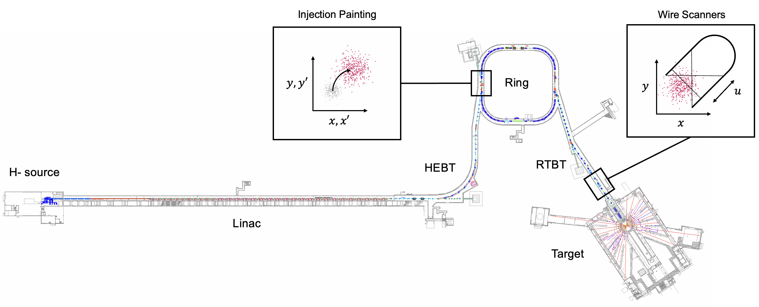
Figure 1: Layout of the Spallation Neutron Source (SNS) accelerator. H- ion minipulses are repeatedly accelerated to 1 GeV in the linac and converted to protons by passing through a carbon foil at the ring injection point. A 700 nanosecond proton pulse is accumulated over 1000 turns in the ring. Dipole magnets vary the mean phase space coordinates ($x$, $x^{\prime}$, $y$, $y^{\prime}$) of the circulating beam relative to the injected beam as a function of time during accumulation. In the Ring-Target Beam Transport (RTBT), four wire scanners measure the particle density on a horizontal, vertical, and diagonal axis ($x$, $y$, $u$).

Each wire scanner consists of three 100-$\mu$m tungsten wires mounted on a fork at forty-five-degree angles relative to each other. The secondary electron emission from each wire gives the beam density on the horizontal ($x$), vertical ($y$), and diagonal ($u$) axis. Each wire scanner operates at 1 Hz repetition rate; thus, each point in the measured profile corresponds to a different beam pulse. A single measurement takes approximately five minutes, including the return to the initial wire position; however, the four wire scanners run in parallel, so each scan generates twelve profiles.

Fig. 2 shows the locations of the wire scanners and nearby quadrupole magnets Fig. 2. Two power supplies control the first eight quadrupoles, while the remaining quadrupoles before the target have independent power supplies. We aim to reconstruct the four-dimensional phase space distribution at a point before the first varied quadrupole (QH18).

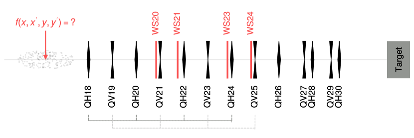
Figure 2: Wire scanner region of the RTBT. Each wire scanner (WS20, WS21, WS23, WS24) contains a horizontal, vertical, and diagonal wire. The faint lines at the bottom of the figure indicate quadrupoles with shared power supplies.

Given a finite number of measurements, it is not entirely clear how to find the optimal set of views—those that place the tightest constraints on the unknown four-dimensional density. Nor is it entirely clear how many views are required to reconstruct the phase space density with sufficient accuracy. These questions deserve further study, especially when the focusing system has coupled or nonlinear elements. Here, we draw on previous experiments in electron accelerators that attempted to reconstruct the four-dimensional phase space distribution from two-dimensional projections onto the $x$-$y$ plane in an uncoupled focusing system. Our focusing system is also uncoupled, and each wire scanner provides three one-dimensional projections that constrain the density in the $x$-$y$ plane. Thus, we hypothesize that observations in these experiments are relevant to us.

Hock and Wolski [11] discovered a near closed-form solution for the four-dimensional phase space density from a set of two-dimensional measurements. The solution assumes independent rotations in the $x$-$x^{\prime}$ and $y$-$y^{\prime}$ planes by the phase advances $\mu_{x}$ and $\mu_{y}$. In other words, in a normalized frame, the transfer matrix takes the form

$$\bm{\mathbf{M}}_{i}=\begin{pmatrix}\phantom{-}\cos\mu_{x_{i}}&\sin\mu_{x_{i}}&0&0\\ -\sin\mu_{x_{i}}&\cos\mu_{x_{i}}&0&0\\ 0&0&\phantom{-}\cos\mu_{y_{i}}&\sin\mu_{y_{i}}\\ 0&0&-\sin\mu_{y_{i}}&\cos\mu_{y_{i}}\end{pmatrix}.$$ (1)

Sampling the entire $\mu_{x}$-$\mu_{y}$ plane leads to an exact solution for $f(x,x^{\prime},y,y^{\prime})$. A lengthy nested scan utilizing this principle has been demonstrated [12]; however, accurate reconstructions appear to be possible without covering the entire range of phase advances. Examples include holding one phase advance fixed while the other varies [4] or varying both phases in a single quadrupole scan [6]. These studies suggest that $\mu_{x}$, $\mu_{y}$, and $\mu_{x}-\mu_{y}$ should cover a range of values between $0$ and $\pi$.

The constraints in the SNS limit our control of the phase advances at each wire scanner. In [13], we found that the nominal optics produce little variation in $\mu_{x}-\mu_{y}$, leading to an ill-conditioned system when fitting the covariance matrix. We found a second set of optics that led to a better-conditioned problem; in the second set of optics, $\mu_{x}$ and $\mu_{y}$ at the last wire scanner (WS24) were shifted by 45 degrees in opposite directions relative to their nominal values. In the present study, we added a third set of optics with different phase advances at WS24. The phase advances at each wire scanner over the three sets of optics are plotted in Fig. 3. We found that this set of optics leads to accurate four-dimensional phase space density reconstructions when tested with known initial distributions.

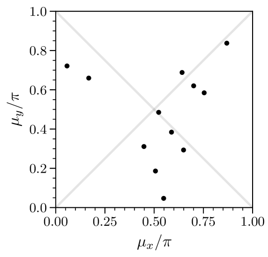
Figure 3: Phase advances from the reconstruction point to each wire scanner. Three sets of optics and four wire scanners per measurement give twelve data points.

We measured a beam generated by a nonstandard injection procedure intended to generate strong cross-plane correlations in the beam. (The standard SNS painting method naturally washes out cross-plane correlations during injection.) We collected beam profiles for three sets of optics in approximately fifteen minutes. Each of the 36 profiles was centered and thresholded to remove background noise. We modeled the accelerator lattice (which contains only drifts and quadrupoles) as a linear transformation of the phase space coordinates. We computed the transfer matrices from the OpenXAL [14] online model of the SNS accelerator.

III Reconstruction Results

As detailed in Appendix A, we performed the reconstruction in two steps. First, we fit the overdetermined covariance matrix to the measured rms beam sizes using Linear Least Squares (LLSQ). Second, we used this covariance matrix to define a Gaussian prior distribution and used the MENT algorithm [15] to maximize the entropy relative to this prior. The result is the most conservative inference from the data.

Fig. 4 shows the LLSQ fit of the covariance matrix to the measured rms beam size on each wire. The fit reproduces the rms beam sizes on all wires in all scan steps. The tightly fit ellipses over a range of phase advances in the $x$-$y^{\prime}$ and $y$-$y^{\prime}$ planes indicate a well-modeled lattice and small measurement errors. Standard LLSQ error propagation gives uncertainties of a few percent for the cross-plane covariances.

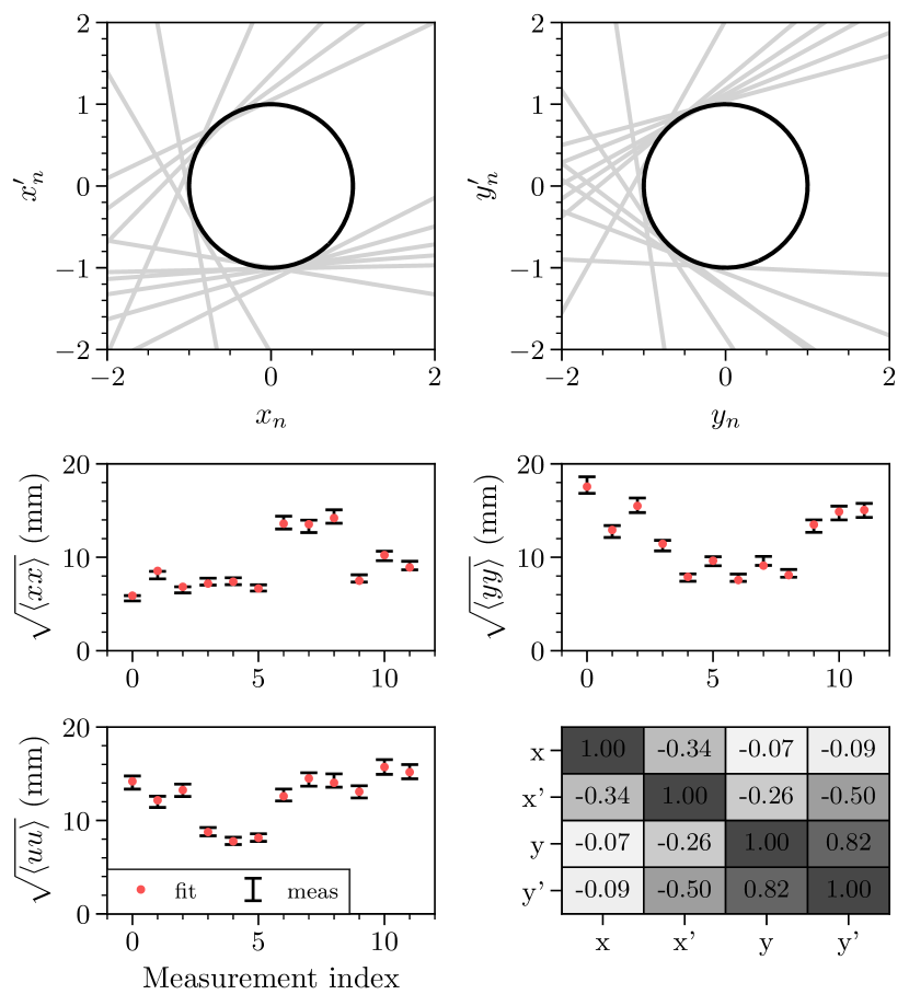
Figure 4: Least-squares covariance matrix fit. Top: vertical lines in $x$-$x^{\prime}$ and $y$-$y^{\prime}$ phase space mapped back to the reconstruction point and plotted in normalized coordinates. In these units, the best-fit ellipse is the unit circle. Bottom: measured (black) vs. fit (red) rms beam sizes on each wire, assuming $5\%$ measurement error. Bottom right: best-fit correlation matrix.

With a Gaussian prior based on the measured covariance matrix, the MENT algorithm converged to the linear-scale profiles in one iteration and the log-scale profiles in another two iterations, terminating at a mean absolute error of $10^{-4}$ per profile. Fig. 5 displays the measured and simulated beam profiles. We would like to highlight the agreement of the profiles down to the $10^{-3}$ level; with improved dynamic range in the wire scanner profiles, MENT may be able to study halo formation processes in two- or four-dimensional phase space. (We do not know if the measured asymmetric tails are real particles or if they are due to background or cross-talk between wires.)

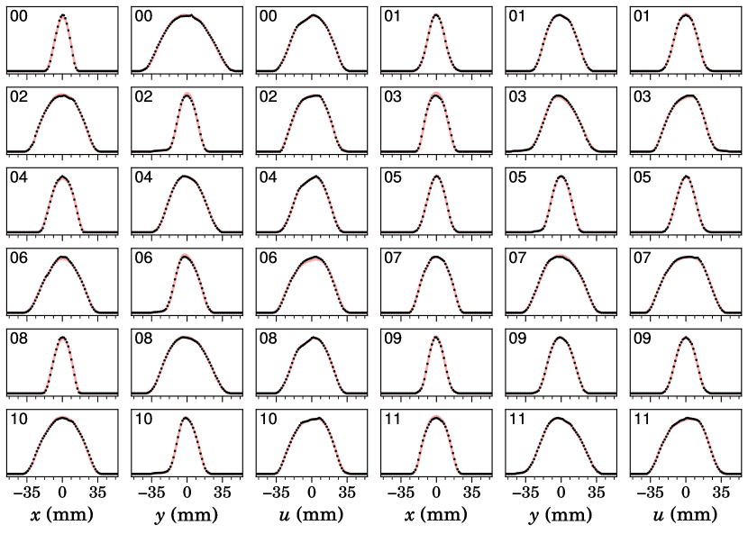
(a)

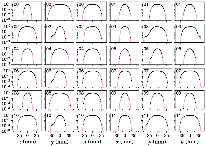
(b)

Figure 5: Measured (black) vs. predicted (red) density on each wire. The measurement index is printed on the top left of each subplot.

Fig. 6 shows the marginal projections of the reconstructed four-dimensional phase space distribution.

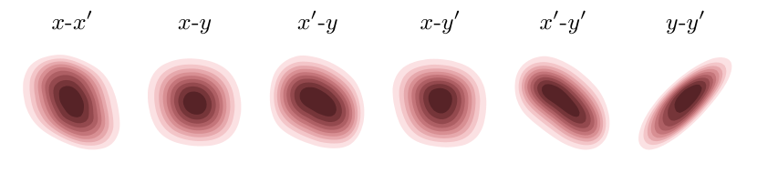
Figure 6: Two-dimensional projections of the reconstructed four-dimensional phase space distribution. Contours vary linearly from $10^{-2}$ to $10^{0}$. A Gaussian filter with $\sigma=1$ pixel is applied to each image.

The nonstandard painting method used in this study ideally generates a uniform density beam with strong linear cross-plane correlations; space charge and other effects blur these correlations and generate a nonuniform density. The remaining linear correlations would be significant if this painting scheme were used for neutron production. In Fig. 7, we see that the average beam density is larger than expected from an uncorrelated beam with the same $x$-$x^{\prime}$ and $y$-$y^{\prime}$ distribution; the accelerator optics would need to be optimized to meet the target specifications. Further examination of the distribution is beyond the scope of this paper.

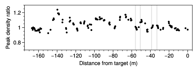
Figure 7: Ratio between the peak density of the reconstructed beam and a decorrelated version of the same beam ($f(x,x^{\prime},y,y^{\prime})\rightarrow f(x,x^{\prime})f(y,y^{\prime})$) as a function of position in the RTBT. Wire scanner locations are gray vertical lines.

The reconstruction quality depends on the accuracy of the forward model, including the measurement process. Our model represents the beamline as a $4\times 4$ transfer matrix:

$$\bm{\mathbf{M}}=\begin{bmatrix}\bm{\mathbf{M}}_{xx}&\bm{\mathbf{M}}_{xy}\\ \bm{\mathbf{M}}_{yx}&\bm{\mathbf{M}}_{yy}\end{bmatrix},$$ (2)

where $\bm{\mathbf{M}}_{xx}$ transforms the $x$-$x^{\prime}$ coordinates, $\bm{\mathbf{M}}_{yy}$ transforms the $y$-$y^{\prime}$ coordinates, and $\bm{\mathbf{M}}_{xy}$ and $\bm{\mathbf{M}}_{yx}$ couple the horizontal and vertical planes. We assume $\bm{\mathbf{M}}_{xy}=\bm{\mathbf{M}}_{yx}=\bm{\mathbf{0}}$ because there are no coupled elements in the RTBT. The following are potential sources of error. (i) The true quadruple coefficients may not be equal to the readback values. We assume these values are accurate because measured twiss parameters typically agree with design values [13]; in future studies, orbit-difference measurements could use BPM data to confirm the linear model accuracy. (ii) Tilted quadrupoles would generate off-block-diagonal terms in the transfer matrix. We expect skew quadrupole components to be negligible, as they can be measured using BPM data [16] and would result in a tilted image on the target during neutron production. (iii) An incorrect beam energy would cause a systematic error in the quadrupole focusing strengths. We ignore this source of error because the beam energy is known to within 0.1% from time of flight measurements in the ring [17]. (iv) The quadrupole coefficients depend on the particle energy—each particle sees a slightly different transverse focusing force—but our model assumes the beam is monoenergetic. Strong transverse-longitudinal correlations in the bunch could amplify the error. The energy spread in the SNS is only a few MeV on top of a 1 GeV synchronous particle energy, so we expect that our model is sufficient. (v) The model does not include space charge. The tune shift over one turn in the ring is approximately 3%, too small to make a difference in the RTBT wire scanner region [13]. (vi) The wire scanner measurements assume the distribution has no pulse-to-pulse variation. Back-to-back measurements show almost no change in the profiles. An electron scanner [8] could also be used to validate this assumption in a future experiment.

It is important to note that tomography is an inverse problem with no unique solution, even with a perfect forward model and noiseless data. MENT returns the most reasonable inference from the data and prior but does not guarantee that the data are informative. (MENT returns the most reasonable solution even in the absence of data.) No existing high-dimensional reconstruction algorithms report uncertainty, so we rely heavily on reconstructions from fake data sets generated by simulated beams that reflect realistic conditions at the reconstruction point. To this end, we generated a test beam using a PyORBIT [18] simulation with parameters qualitatively similar to our experiment. (The simulation was reported in [2].) We rescaled the distribution to match our measured covariance matrix and transported it to the wire scanners using the same transfer matrices as in the experiment. Fig. 8 shows the test results. The reconstructed two-dimensional marginal distributions agree with the true two-dimensional distributions in both the linear correlations (as expected) and nonlinear correlations between planes. This test gives us confidence that MENT generates a reliable inference from the data but also highlights the need for robust uncertainty quantification techniques in real experiments.

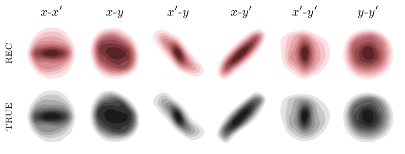
(a)

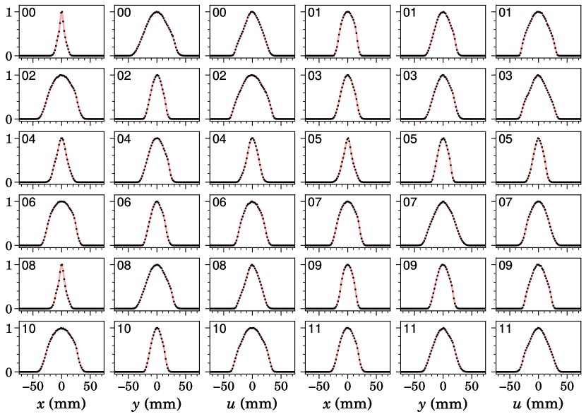
(b)

Figure 8: Reconstruction from fake data. The initial distribution was generated from a PyORBIT simulation with a linear transformation applied to match the $x$-$x^{\prime}$ and $y$-$y^{\prime}$ covariance matrices to the measured values at the reconstruction point (see Fig. 4). The beam was transported to each wire scanner using the same transfer matrices as in the experiment. (a) Reconstructed distribution in normalized coordinates. Contours vary linearly from $10^{-2}$ to $10^{0}$. (b) Simulated (red) vs. “measured” (black) profiles.

IV Conclusion

We have demonstrated four-dimensional phase space tomography using one-dimensional measurements in a high-power hadron ring. We performed the reconstruction using the MENT algorithm with a Gaussian prior defined by the best-fit covariance matrix. The reconstructed distribution reproduces the measured profiles with the same dynamic range as the measurement devices. Test reconstructions with a known ground truth indicate a reasonably small reconstruction uncertainty.

An immediate use for SNS operations is to predict the two-dimensional beam density on the mercury spallation target [19, 20] or planned Second Target Station [21]. A straightforward extension in the SNS is to measure the four-dimensional density as a function of time by extracting the beam on different turns during injection. Such measurements could serve as benchmarks for computer simulations of intense, coupled beam dynamics in hadron rings. Finally, an electron scanner [8] could provide turn-by-turn profiles in the ring; it is unclear if one could use this data to infer the two- or four-dimensional phase space density.

V Acknowledgments

I would like to thank Wim Blockland (ORNL) for troubleshooting the RTBT wire scanners, the SNS accelerator operators for enabling these studies, and Andrei Shishlo (ORNL) for carefully reading this manuscript.

This manuscript has been authored by UT Battelle, LLC under Contract No. DE-AC05-00OR22725 with the U.S. Department of Energy. The United States Government retains and the publisher, by accepting the article for publication, acknowledges that the United States Government retains a non-exclusive, paid-up, irrevocable, world-wide license to publish or reproduce the published form of this manuscript, or allow others to do so, for United States Government purposes. The Department of Energy will provide public access to these results of federally sponsored research in accordance with the DOE Public Access Plan (http://energy.gov/downloads/doe-public-access-plan).

Appendix A Reconstruction method

We aim to infer the probability density function $f(\bm{\mathbf{v}})$ from a set of one-dimensional projections, where $\bm{\mathbf{v}}=(v_{1},\dots,v_{N})$ is the phase space coordinate vector. (In four-dimensional phase space, $\bm{\mathbf{v}}=(x,x^{\prime},y,y^{\prime})$, where $x$ and $y$ are the positions and $x^{\prime}$ and $y^{\prime}$ are the momenta.) We assume the $i$th projection is measured after a linear transformation

$$\bm{\mathbf{w}}_{i}=\bm{\mathbf{M}}_{i}\bm{\mathbf{v}},$$ (3)

where $\bm{\mathbf{M}}_{i}$ is an $N\times N$ matrix representing the accelerator transport between the reconstruction point and the measurement device. We measure the one-dimensional projected density $g_{i}(w_{ij})$, where $w_{ij}$ is the $j$th dimension of $\bm{\mathbf{w}}_{i}$. Thus, the distribution must satisfy the following constraints:

$$g_{i}(w_{ij})-\int f(\bm{\mathbf{v}}(\bm{\mathbf{w}}_{i}))\prod_{k\neq j}dw_{ik}=0$$ (4)

Entropy maximization (MaxEnt) provides a logically consistent way to incorporate prior information in the reconstruction and identify a unique solution from the many that satisfy Eq. (4). MaxEnt updates a prior distribution $f_{*}(\bm{\mathbf{v}})$ to a posterior by maximizing the relative entropy

$$S[f(\bm{\mathbf{v}}),f_{*}(\bm{\mathbf{v}})]=-\int f(\bm{\mathbf{v}})\log\left(\frac{f(\bm{\mathbf{v}})}{f_{*}(\bm{\mathbf{v}})}\right)d\bm{\mathbf{v}},$$ (5)

subject to Eq. (4). The method of Lagrange multipliers leads to the following form of the posterior:

$$f(\bm{\mathbf{v}})=f_{*}(\bm{\mathbf{v}})\prod_{i}\exp(\lambda_{i}(w_{ij})),$$ (6)

where $\lambda_{i}(w_{ij})$ are unknown Lagrange multiplier functions. The MENT algorithm uses a nonlinear Gauss-Seidel relaxation method to find $\lambda_{i}$ such that the distribution in Eq. (6) satisfies the constraints in Eq. (4). We use a sampling-based method to implement the Gauss-Seidel iterations; this will be reported in a separate paper.

An advantage of the MENT approach is its incorporation of external information through $f_{*}(\bm{\mathbf{v}})$. We note that the $N\times N$ covariance matrix ${\bm{\mathbf{\Sigma}}}=\langle\bm{\mathbf{v}}\bm{\mathbf{v}}^{T}\rangle$ is overdetermined by the measured beam profiles. Thus, we assume a Gaussian prior of the form

$$f_{*}(\bm{\mathbf{v}})=\left[\frac{1}{(2\pi)^{N}|\bm{\mathbf{\hat{\Sigma}}}|}\right]^{1/2}\exp\left(-\frac{1}{2}\bm{\mathbf{v}}^{T}\hat{\bm{\mathbf{\Sigma}}}^{-1}\bm{\mathbf{v}}\right),$$ (7)

where $\hat{\bm{\mathbf{\Sigma}}}$ is the best-fit covariance matrix determined by the following procedure. Under the symplectic linear transformation $\bm{\mathbf{M}}_{i}$, $\bm{\mathbf{\Sigma}}$ transforms as

$$\mathbf{\Sigma}\rightarrow\mathbf{M}_{i}\mathbf{\Sigma}\mathbf{M}_{i}^{T}.$$ (8)

Eq. (8) linearly relates the measured rms beam size $\eta_{i}=\langle w_{ij}^{2}\rangle$ to the lower-triangular elements $\bm{\mathbf{\sigma}}$ of the initial covariance matrix. Stacking the measurements into a single vector $\bm{\mathbf{\eta}}=(\eta_{1},\eta_{2},\dots)$ gives the following system of equations:

$$\bm{\mathbf{A}}\bm{\mathbf{\sigma}}=\bm{\mathbf{\eta}}.$$ (9)

We generate a solution $\hat{\bm{\mathbf{\sigma}}}$ (and therefore $\hat{\bm{\mathbf{\Sigma}}}$) to Eq. (9) using ordinary linear least squares (LLSQ) [22]:

$$\hat{\bm{\mathbf{\sigma}}}=(\bm{\mathbf{A}}^{T}\bm{\mathbf{A}})^{-1}\bm{\mathbf{A}}^{T}\bm{\mathbf{\eta}}.$$ (10)

With the LLSQ fit in hand, we may run the MENT algorithm to reconstruct the beam distribution in normalized phase space coordinates,

$$\bm{\mathbf{z}}=\bm{\mathbf{T}}^{-1}\bm{\mathbf{v}},$$ (11)

such that $\langle\bm{\mathbf{z}}\bm{\mathbf{z}}^{T}\rangle=\bm{\mathbf{I}}$. When reconstructing in normalized two-dimensional phase space, the projection angles in the $x$-$x^{\prime}$ plane are equivalent to the betatron phase advances; this is advantageous because the phase advances between measurement locations are often approximately equal [11]. In practice, reconstructing in normalized space involves only appending the unnormalizing matrix $T$ to each transfer matrix:

$$\bm{\mathbf{M}}_{i}\rightarrow\bm{\mathbf{M}}_{i}\bm{\mathbf{T}}.$$ (12)

References

- Cathey et al. [2018] B. Cathey, S. Cousineau, A. Aleksandrov, and A. Zhukov, First six dimensional phase space measurement of an accelerator beam, Phys. Rev. Lett. 121, 064804 (2018).
- Holmes et al. [2018] J. A. Holmes, T. Gorlov, N. J. Evans, M. Plum, and S. Cousineau, Injection of a self-consistent beam with linear space charge force into a ring, Phys. Rev. Accel. Beams 21, 124403 (2018).
- Danilov and Nagaitsev [2010] V. Danilov and S. Nagaitsev, Nonlinear accelerator lattices with one and two analytic invariants, Phys. Rev. ST Accel. Beams 13, 084002 (2010).
- Wolski et al. [2020] A. Wolski, D. C. Christie, B. L. Militsyn, D. J. Scott, and H. Kockelbergh, Transverse phase space characterization in an accelerator test facility, Phys. Rev. Accel. Beams 23, 032804 (2020).
- Wolski et al. [2022] A. Wolski, M. A. Johnson, M. King, B. L. Militsyn, and P. H. Williams, Transverse phase space tomography in an accelerator test facility using image compression and machine learning, Phys. Rev. Accel. Beams 25, 122803 (2022).
- Roussel et al. [2023] R. Roussel, A. Edelen, C. Mayes, D. Ratner, J. P. Gonzalez-Aguilera, S. Kim, E. Wisniewski, and J. Power, Phase space reconstruction from accelerator beam measurements using neural networks and differentiable simulations, Phys. Rev. Lett. 130, 145001 (2023).
- Wong et al. [2022] J. C. Wong, A. Shishlo, A. Aleksandrov, Y. Liu, and C. Long, 4d transverse phase space tomography of an operational hydrogen ion beam via noninvasive 2d measurements using laser wires, Phys. Rev. Accel. Beams 25, 042801 (2022).
- Blokland et al. [2009] W. Blokland, S. Aleksandrov, S. Cousineau, D. Malyutin, and S. Starostenko, Electron scanner for SNS ring profile measurements, Proceedings of DIPAC09, TUOA03, Basel, Switzerland (2009).
- Minerbo et al. [1981] G. N. Minerbo, O. R. Sander, and R. A. Jameson, Four-dimensional beam tomography, IEEE Transactions on Nuclear Science 28, 2231 (1981).
- Henderson et al. [2014] S. Henderson et al., The Spallation Neutron Source accelerator system design, Nuclear Instruments and Methods in Physics Research Section A: Accelerators, Spectrometers, Detectors and Associated Equipment 763, 610 (2014).
- Hock and Wolski [2013] K. M. Hock and A. Wolski, Tomographic reconstruction of the full 4D transverse phase space, Nuclear Instruments and Methods in Physics Research, Section A: Accelerators, Spectrometers, Detectors and Associated Equipment 726, 8 (2013).
- Jaster-Merz et al. [2024] S. Jaster-Merz, R. W. Assmann, R. Brinkmann, F. Burkart, W. Hillert, M. Stanitzki, and T. Vinatier, 5d tomographic phase-space reconstruction of particle bunches, Phys. Rev. Accel. Beams 27, 072801 (2024).
- Hoover and Evans [2022] A. Hoover and N. Evans, Four-dimensional emittance measurement at the Spallation Neutron Source, Nuclear Instruments and Methods in Physics Research Section A: Accelerators, Spectrometers, Detectors and Associated Equipment 1041, 167376 (2022).
- Zhukov et al. [2022] A. Zhukov et al., Openxal status report 2022, in Proc. 13th International Particle Accelerator Conference, International Particle Accelerator Conference No. 13 (JACoW Publishing, Geneva, Switzerland, 2022) pp. 1271–1274.
- Minerbo [1979] G. Minerbo, Ment: A maximum entropy algorithm for reconstructing a source from projection data, Computer Graphics and Image Processing 10, 48 (1979).
- Pelaia and Cousineau [2008] T. Pelaia and S. Cousineau, A method for probing machine optics by constructing transverse real space beam distributions using beam position monitors, Nuclear Instruments and Methods in Physics Research Section A: Accelerators, Spectrometers, Detectors and Associated Equipment 596, 295 (2008).
- Wong et al. [2021] J. C. Wong, A. Aleksandrov, S. Cousineau, T. Gorlov, Y. Liu, A. Rakhman, and A. Shishlo, Laser-assisted charge exchange as an atomic yardstick for proton beam energy measurement and phase probe calibration, Phys. Rev. Accel. Beams 24, 032801 (2021).
- Shishlo et al. [2015] A. Shishlo, S. Cousineau, J. Holmes, and T. Gorlov, The particle accelerator simulation code PyORBIT, Procedia Computer Science 51, 1272 (2015), international Conference On Computational Science, ICCS 2015.
- Blokland [2014] W. Blokland, Experience with and studies of the SNS target imaging system, Proc. of IBIC , 447 (2014).
- Radaideh et al. [2022] M. I. Radaideh, L. Lin, H. Jiang, and S. Cousineau, Bayesian inverse uncertainty quantification of the physical model parameters for the Spallation Neutron Source First Target Station, Results in Physics 36, 105414 (2022).
- Galambos et al. [2015] J. Galambos et al., Technical Design Report, Second Target Station 10.2172/1185891 (2015).
- Prat and Aiba [2014] E. Prat and M. Aiba, Four-dimensional transverse beam matrix measurement using the multiple-quadrupole scan technique, Physical Review Special Topics - Accelerators and Beams 17, 10.1103/PhysRevSTAB.17.052801 (2014).