Physically constrained quantum clock-driven dynamics

Abstract

Thermal machines are physical systems specifically designed to make thermal energy available for practical use through state transformations in a cyclic process. This concept relies on the presence of an additional element equipped with a clock, controlling which interaction Hamiltonian between the system and the reservoirs must act at a certain time and that remains unaffected during this process. In the domain of quantum dynamics, there is substantial evidence to suggest that fulfilling this final condition is, in fact, impossible, except in ideal and far-from-reality cases. In this study we start from one such idealized condition and proceed to relax the primary approximations to make the model more realistic and less ideal. The main result is a fully quantum description of the engine-clock dynamics within a realistic quantum framework. Furthermore, this approach offers the possibility to address the deeper and more fundamental challenge of defining meaningful time operators in the realm of quantum mechanics from a different standpoint.

I Introduction

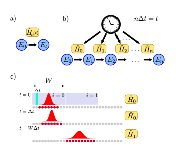
Figure 1: Autonomous clock-driven quantum machine. a) The engine evolves from the state $E_{0}$ to the state $E_{t}$ under the action of a propagator generated by the time-dependent Hamiltonian $\hat{H}_{E}(t)$. b) The time-dependent Hamiltonian is represented by a series of time-independent Hamiltonians, with the addition of a clock mechanism that chooses the appropriate generator at each intermediate stage of the time evolution. Together, the engine and clock form an autonomous system. c) A gaussian pulse travelling on a line acts as clock by selecting the generator of the evolution of the engine. The switching process relies on the field’s intensity within a time interval of magnitude $W$, which serves as a measurement of the pulse’s “position”. The field is decomposed into a succession of noninteracting time-bin ancillae. For the sake of simplicity we render the clock degradation process as a pure broadening of the pulse.

An engine can generally be defined as an open system coupled to many portions of the surrounding environment, which act as reservoirs. The primary aim of an engine is generating power in the form of mechanical work Cangemi et al. (2023). The realization of thermodynamic cycles, whether classical or quantum, relies on time-dependent Hamiltonians, which often incur significant energy costs that are difficult to fully capture in theoretical models. This problem can be addressed by embedding the system within an expanded framework that includes an additional “clock” system to keep track of time. The engine and clock together evolve under a time-independent Hamiltonian in a larger Hilbert space Aharonov and Bohm (1961). While this approach increases the dimensionality and complexity of the system due to the expanded Hilbert space, it compensates by making the overall dynamics autonomous, removing the need for external time-dependent driving. This framework has offered valuable insights into how the intrinsic physics of the time-keeping system Woods et al. (2018); Woods and Horodecki (2023) and the process of time sampling Meier et al. (2024); Erker et al. (2017); Xuereb et al. (2023) affect the dynamics of generic quantum machines, with notable implications for quantum computing protocols Feynman (2018, 1985); Lloyd (1996); Watkins et al. (2024); De Falco and Tamascelli (2004); Woods (2024). Additionally, this perspective has become foundational in the resource theory of thermodynamics Horodecki and Oppenheim (2013). In the most general framework, a quantum system that can either access or generate a time signal and use it to control the evolution of another system, while remaining robust to perturbations (such as back reactions from the engine), can serve as a clock Woods et al. (2018). A minimal model including effectively all these features has been recently proposed in Malabarba et al. (2015): the time-dependent Hamiltonian coupling system and environment is modelled as a set of time-independent operators acting sequentially during the evolution time. Each operator is correlated to the position of an external particle (the clock) freely moving under a Hamiltonian that is assumed to be linear in the momentum. The control mechanism is provided by an effective coupling between the particle and the engine that is assumed to commute with the free Hamiltonian of the engine (covariant operation). As pointed out in Woods and Horodecki (2023), this model is inherently nonphysical because of the particular free evolution assumed for the clock (pure translation), that requires an unbounded clock Hamiltonian. This argument can be seen as another facet of the celebrated Pauli objection to the existence of a time operator in standard quantum mechanics Pauli et al. (1980); Hilgevoord (2005). Namely, the equation of motion of a self-adjoint time operator $\hat{T}$ reads

$$\dot{\hat{T}}=i[\hat{H},\hat{T}]=\mathbb{1}\,\Rightarrow[\hat{T},\hat{H}]=i\mathbb{1}\,,$$ (1)

thus if such operators were to exist, they would need to be unitarily equivalent to $\hat{x}$ and $\hat{p}$, implying that their spectra are continuous and unbounded from below. This situation would result in unstable and nonphysical descriptions of interacting quantum theories. In essence, the commutation relation involving $\hat{T}$ and the Hamiltonian operator, as outlined in Eq. (1), lacks exact physical solutions within the framework of standard non-relativistic quantum mechanics. This issue has deep historical roots within the genesis of quantum theory Hilgevoord (2005). Over the years, various strategies have emerged to confront this challenge, each presenting distinctive viewpoints. These strategies include the proposition of non-self-adjoint time operators Olkhovsky et al. (1974), as well as explorations within the framework of relativistic quantum field theory Bauer (2014). Remarkably, an alternative perspective has advocated for the retention of unbounded operators Leon and Maccone (2017). Other attempts in the literature, as documented in Woods et al. (2018); Woods and Horodecki (2023), often rely on reasonable finite-dimensional approximations of $\hat{T}$. In this study, we extend the ideal model presented in Malabarba et al. (2015) to encompass a realistic quantum framework, addressing complexities previously unaccounted for. Specifically, our approach involves utilizing a quantum field as our clock-system and tracking time by monitoring the motion of a coherent pulse as it propagates along a linear trajectory. Under the same fundamental assumptions as in Malabarba et al. (2015) regarding the coupling Hamiltonian between the system and the engine, we demonstrate that this coupling directly influences the dispersion law of the wave-packet, resulting in a significant deterioration of the clock’s performance. This result paves the way to address the challenge of approximating the solution of Eq. (1) by means of infinite-dimensional operators that form an integral part of the model.

The paper is structured as follows: in Sec. II we define the global model of engine and clock and describe the dynamics of the system using the framework of quantum collision models (QCM) Ciccarello (2018); Gross et al. (2018); Ciccarello et al. (2022). Subsequently, in Sec. B we introduce a model for the interaction between the control system and the engine. This model, designed for situations characterized by minor degradation, serves to restrict deviations from the desired dynamics we aim to implement. Sec. III explicitly addresses the issue of degradation and in Sec. IV we return to the problem of time operators to quantitatively assess how the unavoidable degradation of physical clocks affects the precise definition of time operators in QM.

II Definition of engine and clock

Following the reasoning in Malabarba et al. (2015) we consider a bipartite Hilbert space $\mathcal{H}=\mathcal{H}_{E}\otimes\mathcal{H}_{C}$, where $E$ identifies a generic open system and its surrounding environment, and $C$ an auxiliary system denoted as clock. The role of the clock is controlling the evolution of the system without any external control. The total Hamiltonian reads

$$\hat{H}_{\rm tot}=\hat{H}_{E}+\hat{H}_{C}+\hat{V}_{EC}\,,$$ (2)

where $H_{E}$ and $H_{C}$ are the free Hamiltonians of engine and clock, respectively. The identities over the complementary Hilbert spaces are omitted. In Malabarba et al. (2015) the interaction between engine and clock takes the form

$$\hat{V}_{EC}=\int_{\mathbb{R}}\!\!\!dx\,\hat{V}_{E}(x)\otimes\ket{x}\!_{C}\!\bra{x}\,,$$ (3)

where $\ket{x}\!_{C}\!\bra{x}$ projects over the different position states of the clock and $\hat{V}_{E}\in\mathcal{H}_{E}$. We choose as a clock a one-dimensional bosonic field with free Hamiltonian

$$\hat{H}_{C}=\int\!dk\,\omega_{k}\hat{a}_{k}^{\dagger}\hat{a}_{k}\,.$$ (4)

In the position space, the initial state of the clock is a pulse described by

$$\ket{\psi}^{(0)}_{C}=\int dx\,\xi_{x_{0}}(x)\,\mathcal{X}(\hat{a}^{\dagger}_{x})\,\ket{\rm{vac}}\equiv\hat{\psi}^{{\dagger}}_{C}(x_{0})\ket{\rm{vac}}\,,$$ (5)

where $\xi_{x_{0}}(x)$ is the pulse envelope function centered on $x_{0}$, with velocity $c=1$ and $\mathcal{X}$ is an operator acting on the Fourier-transformed ladder operators of the field $\hat{a}^{\dagger}_{x}$ (e.g. displacement or squeezing). Within the quasimonochromatic approximation Baragiola et al. (2012), i.e. the spectral width is much smaller than the average frequency of the wave-packet. In the following, we will assume a linear dispersion relation $\omega_{k}=v_{g}k$ in the free Hamiltonian Eq. (4). These assumptions correspond to taking as our clock a single-photon pulse traveling in a vacuum or a particle with a very narrow distribution in momentum. For simplicity, we assume a gaussian envelope with frequency bandwidth $\Omega$

$$\xi(x)=\left(\frac{\Omega^{2}}{2\pi}\right)^{1/4}e^{-\Omega^{2}(x-x_{0})^{2}/4}\,,$$ (6)

with $\mathcal{X}=\mathcal{I}$, where $\mathcal{I}$ is the identity map, i.e. a single-particle pulse.

We can distinguish between two different times only when the pulse has moved by an amount that is larger than its width (in Fig. 1 there’s an example of this process). This leads naturally to a first discretisation of the interaction defined by a time window of size $W$ and discretising $\hat{V}_{E}(s)$ on them. In light of this intuition we make the following replacements in Eq. (3):

$$\hat{V}_{E}(s) \rightarrow\sum_{i}\hat{V}_{E}(s_{i})\Theta_{W}(s-s_{i})\,,$$ (7)

$$|s\rangle_{C}\langle s| \rightarrow\frac{1}{W}\int_{\mathcal{D}_{s}}dx~{}\hat{a}^{\dagger}_{x}\hat{a}_{x}\,,$$ (8)

where $\Theta(s-s_{i})$ is the rectangle function of size $W$ centered on the time $s_{i}$, which can be chosen among the times within the $i$th window. We denote with $\mathcal{D}_{q}$ the integration range corresponding to a time window centered on the value $q$. Let’s assume that $s_{i}$ corresponds to the centre of the window. In the second equation the measure of position is defined, i.e. we integrate the number of excitations per length over the region corresponding to $s$. More detailed information about $W$ and the discrete potential $\hat{V}(s_{i})$ will come in subsequent sections.

Plugging Eqs. (7) and (8) into Eq.(3), the interaction term can be expressed as

$$\hat{V}_{EC}\rightarrow \int_{\mathbb{R}}ds\sum_{i}\hat{V}_{e}(s_{i})\Theta_{W}(s-s_{i})\otimes\frac{1}{W}\int_{\mathcal{D}_{s}}dx~{}\hat{a}^{\dagger}_{x}\hat{a}_{x}$$

$$=\frac{1}{W}\sum_{i}\hat{V}_{e}(s_{i})\otimes\int_{\mathbb{R}}ds\Theta_{W}(s-s_{i})\int_{\mathcal{D}_{s}}dx~{}\hat{a}^{\dagger}_{x}\hat{a}_{x}$$

$$=\frac{1}{W}\sum_{i}\hat{V}_{e}(s_{i})\otimes\int_{\mathcal{D}_{i}}dx~{}\hat{a}^{\dagger}_{x}\hat{a}_{x}\,,$$ (9)

where $\mathcal{D}_{i}$ is now the region including $s_{i}$ (following the previous assumption it is $[s_{i}-W/2,s_{i}+W/2]$).

In the interaction picture with respect to the free Hamiltonian of the clock and the engine, we have

$$\hat{V}_{EC}^{I}(t)=\frac{1}{W}\sum_{i}\hat{V}^{I}_{E}(s_{i})\otimes\int_{\mathcal{D}_{i}}dx~{}\hat{a}^{\dagger}_{x-t}\hat{a}_{x-t}\,,$$ (10)

with $\hat{V}^{I}_{E}(s_{i})=e^{i\hat{H}_{E}t}\hat{V}_{E}(s_{i})e^{-i\hat{H}_{E}t}$ (we omit the time dependence) and the total propagator is given by

$$\hat{\mathcal{U}}_{t,0}=e^{-i(\hat{H}_{E}+\hat{H}_{C})t}\mathcal{T}\exp\left\{-i\int_{0}^{t}~{}d\tau\hat{V}^{I}_{EC}(\tau)\right\}\,,$$ (11)

where $\mathcal{T}$ is the time ordering operator.

We now discretise the time axis into shorter intervals $t=n\Delta t$ with $n\in\mathbb{N}$ and the time step $\Delta t\ll W$. Thus the propagator in Eq. (11) is decomposed as

$$\hat{\mathcal{U}}_{t,0} =\prod_{n}\hat{\mathcal{U}}_{n}$$

$$=\prod_{n}e^{-i(\hat{H}_{E}+\hat{H}_{C})\Delta t}\mathcal{T}\exp\left\{-i\int_{t_{n-1}}^{t_{n}}~{}d\tau\hat{V}^{I}_{EC}(\tau)\right\}\,.$$ (12)

In the limit of $\Delta t\rightarrow 0$ we can approximate the propagator (12) through the first order of the Magnus expansion Magnus (1954):

$$\mathcal{H}_{n}^{(0)} =\frac{1}{\Delta t}\frac{1}{W}\sum_{i}\hat{V}_{e}^{I}(s_{i})\otimes\int_{\mathcal{D}_{i}}dx~{}\int_{t_{n-1}}^{t_{n}}~{}d\tau\hat{a}^{\dagger}_{x-\tau}\hat{a}_{x-\tau}$$

$$=\frac{1}{W}\sum_{i}\hat{V}^{I}_{e}(s_{i})\otimes\int_{t_{i}-W/2-t_{n}}^{t_{i}+W/2-t_{n}}dx~{}\delta\hat{n}_{x}$$

$$=\frac{1}{W}\sum_{i}\hat{V}^{I}_{e}(s_{i})\otimes\hat{N}_{W(i+1/2)-n}\,,$$ (13)

where $\delta\hat{n}_{\alpha}:=\frac{1}{\Delta t}\int_{t_{n-1}}^{t_{n}}~{}d\tau\hat{a}^{\dagger}_{\alpha-\tau}\hat{a}_{\alpha-\tau}$ and $\hat{N}_{W(i+1/2)-n}:=\int_{t_{i}-W/2-t_{n}}^{t_{i}+W/2-t_{n}}dx~{}\delta\hat{n}_{x}$. Thus we obtain the discrete-time propagator

$$\hat{\mathcal{U}}_{n}\simeq e^{-i(\hat{H}_{e}+\hat{H}_{c})\Delta t}\exp\left\{-\frac{i\Delta t}{W}\sum_{i}\hat{V}^{I}_{e}(s_{i})\otimes\hat{N}_{W(i+1/2)-n}\right\}\,.$$ (14)

Note that in our approximation we used the operator in Eq. (8) instead of the field operator $\hat{\psi}^{{\dagger}}_{c}(s)\hat{\psi}_{c}(s)$ to avoid biasing by the shape of the pulse. None of the previous assumptions prevent pulse broadening, as it depends on the clock-engine interaction Hamiltonian. Note that unlike the ideal scenario proposed in Malabarba et al. (2015), we cannot decompose the propagator in Eq.(14) into two separate operators for the clock and the engine. Consequently, the engine and the clock exhibit correlations during their evolution. This back-reaction affects the clock’s state and provides the physical basis for degradation.

III Clock degradation and dispersion law

The free evolution of the clock ladder operators reads

$$e^{i\hat{H}_{C}t}\hat{a}_{x}e^{-i\hat{H}_{C}t}=\hat{a}_{x-t}\,,$$ (15)

i.e. the free Hamiltonian of the clock only translates the state of the field. It becomes evident that when the clock evolves exclusively under this Hamiltonian with the assumption of a linear dispersion, it might behave as an ideal clock in the sense of Woods et al. (2018). Consequently, we can explore the potential for degradation by examining the emergence of nonlinearity in the dispersion law. Starting from Eq. (9) we have, in the Fourier space

$$\hat{H}_{C}+\hat{V}_{EC} =\int dkv_{g}k\mathbb{1}_{E}\hat{a}^{\dagger}_{k}\hat{a}_{k}$$

$$+\int dkdk^{\prime}\mathcal{F}[\hat{V}_{E}](k-k^{\prime})\otimes\hat{a}^{\dagger}_{k}\hat{a}_{k^{\prime}}\,,$$ (16)

where $\mathcal{F}[\hat{V}_{E}](k)=\int dx\hat{V}_{E}(x)e^{-ikx}$ denotes the Fourier transform of the engine Hamiltonian. Even in the case in which $\langle\mathcal{F}[\hat{V}_{E}]\rangle_{E}\propto f(k,t)\delta(k-k^{\prime})$, the interaction term still introduces a complex and non-trivial deviation from linearity into the dispersion relation. One of the consequences of the non-linearity of the dispersion relation is wave-packet broadening Diels and Rudolph (2006) . When the wave-packet width becomes comparable to $W$, from the point of view of the engine’s dynamics, we are not able to select which of the transformations is the one we must implement to reproduce the target dynamics: in other words, we do not know what time it is. We interpret this phenomenon as a manifestation of clock degradation arising from the interaction with the engine. This interaction leads to the emergence of an effective mass $\propto(\partial^{2}_{k}\omega_{k})^{-1}$, even when the free clock field is originally massless. On the other hand, the coupling (9) is a translation of (3) for quantum fields, which in turn finds its origins in the broader concept of the ancilla-clock system initially introduced in Horodecki and Oppenheim (2013). Therefore, for clocks falling within this broad class, our findings provide direct evidence of the intrinsic connection between degradation and the effective mass of the system operating as a clock. Directly solving the clock’s dynamics under Eq. (16) in order to quantify the effects of degradation is unpractical. In the next section we take advantage of our model to introduce a time operator formalism that will enable us to achieve a comprehensive characterization of clock degradation.

IV Time operators

Inspired by the functional form of the Hamiltonian in Eq.(9), we define a continuous clock time operator

$$\hat{T}=\frac{1}{c}\int dx\,x\,\hat{a}_{x}^{\dagger}\hat{a}_{x}\,,$$ (17)

where $c$ is the speed of light in the vacuum. It is interesting to note that given any continuous dispersion relation $\omega(k)$ for the clock system, we can find an expression for the corresponding Eq. (1), as shown by the following

Theorem IV.1.

Given the time operator defined above, and given a continuous dispersion relation $\omega(k)$, the commutator with $\hat{H}_{C}$ reads

$$[\hat{T},\hat{H}_{C}]=i\hat{\Lambda}$$

where

$$\hat{\Lambda}=\frac{1}{c}\int dk\,\omega^{\prime}(k)\hat{a}_{k}^{\dagger}\hat{a}_{k}\,,$$ (18)

with $\omega^{\prime}(k)=d\omega(k)/dk$.

Proof.

See Appendix A. ∎

The theorem above implies the Heisenberg equation of motion

$$\dot{\hat{T}}_{H}(t)=i[\hat{T}_{H}(t),\hat{H}_{C}]=\int dk\,\omega^{\prime}(k)\hat{a}_{k}^{\dagger}\hat{a}_{k}=\hat{\Lambda}\,,$$ (19)

which is generally far off from the ideal case of Eq. (1), and the clock states will in general spread, a phenomenon that causes superpositions of different time states and reduces the resourcefulness of the clock system. Having introduced a time operator, we are in the position of defining an associated quantifier of degradation by means of the variance of the operator $\hat{T}$:

Definition IV.1 (Clock degradation).

Given a time operator $\hat{T}$ and an initial clock state $\ket{\psi_{C}}$, the degradation $D(t)$ of the clock is defined as

$$D(t)=\sqrt{\text{Var}(\hat{T})}=\left(\langle\hat{T}^{2}\rangle-\langle\hat{T}\rangle^{2}\right)^{\frac{1}{2}}\,.$$

Given a dispersion relation and its corresponding modified Heisenberg algebra $[\hat{T},\hat{H}_{C}]=i\hat{\Lambda}$, we find that the time dependency of $D(t)$ can be extracted: it is linear for any (continuous) choice of dispersion relation $\omega(k)$, and proportional to the variance of the operator $\hat{\Lambda}$:

Theorem IV.2.

Given a dispersion relation $\omega(k)$, and its corresponding modified commutator $[\hat{T},\hat{H}_{C}]=i\hat{\Lambda}$, the clock degradation obeys

$$D(t)=\sqrt{\rm{Var}(\hat{\Lambda})}~{}t$$

Proof.

See Appendix A. ∎

The theorem above suggests that it might always be possible to completely eliminate the problem of degradation at all future times by preparing initial clock states such that $\text{Var}(\hat{\Lambda})=0$, i.e. eigenstates of $\hat{\Lambda}$. Interestingly enough, under fairly general assumptions this possibility is ruled out, except in the case of strictly linear dispersion relation, as shown by the following

Theorem IV.3.

Given a single-particle clock state $\ket{\psi_{C}}$, whose support in $k$-space is defined by a compact interval $\Omega\in\mathbb{R}$ with non-zero length, and given a continuous and injective dispersion relation $\omega(k):\Omega\to\mathbb{R}$, one has $D(t)=0$ $\forall t$ if and only if $\omega(k)$ is linear in the whole support $\Omega$.

Proof.

See Appendix A. ∎

As a corollary to the theorem above, we can consider the limit case in which our initial clock state is extremely well localised in a spatial window of width $W$. Since good clock states must be sufficiently localised in position, they must necessarily be sufficiently delocalised in momentum and therefore the support $\Omega$ in the theorem above becomes the whole real line as $W\to 0$, forcing the dispersion relation to be linear everywhere.
We can now investigate what happens to Eq. (1) in the case of a linear dispersion relation $\omega(k)=ck$. Following the results above one has

$$\hat{\Lambda}=\int dk\,\hat{a}_{k}^{\dagger}\hat{a}_{k}=\hat{N}_{C}\,,$$ (20)

where $\hat{N}_{C}$ counts the excitations of the field. Remarkably, this is the unique case in which we can construct resourceful clock pulses that have $\text{Var}(\hat{\Lambda})=0$ but are not eigenstates of the clock Hamiltonian (rendering their resourcefulness as clock states void, due to their stationarity). The initial state of the clock Eq. (5) has a fixed number of excitations $N$, and furthermore such number of excitations is exactly conserved during the dynamics due to the fact that $[\hat{N}_{C},\hat{H}]=0$. Thus, within our assumptions, when starting from a clock state with well-defined particle number $\hat{N}_{C}\ket{\psi_{C}}=N\ket{\psi_{C}}$, we can always define a rescaled time operator by introducing the projector $\mathbb{P}_{N}$ onto the $N$-particles sector

$$\hat{\tau}=\frac{1}{N}\hat{\mathbb{P}}_{N}\hat{T}\hat{\mathbb{P}}_{N}$$ (21)

such that

$$\dot{\hat{\tau}}=\mathbb{1}_{N}\,,$$ (22)

that corresponds to the original Pauli relation in the $N$ excitation subspace. This definition allows us to conclude that, as long as the joint clock-engine dynamics does not couple sectors with different number of particles, the Pauli relation can be obeyed exactly if the effective dispersion relation of the clock after being coupled to the engine can be maintained linear. In other words, as expected, we found that any wave-packet with a fixed total number of excitations traveling through a medium with linear dispersion law (i.e. any massless wavepacket) behaves as an ideal clock, in the sense of Malabarba et al. (2015). However, as pointed out in the previous section, this is fundamentally impossible, due to the fact that the interaction with the engine will inevitably correct the bare dispersion relation of the clock, generating a finite effective mass and thus introducing unavoidable degradation of any clock state that is sufficiently localised in position. This trade-off between degradation and resourcefulness of the clock states is a consequence of the Heisenberg uncertainty relation for the clock’s position and momentum, and can then be translated into a lower-bound

$$D(t)\geq\frac{|\langle\hat{\Lambda}\rangle|}{2\,\Delta\hat{H}_{C}},$$ (23)

where $\Delta\hat{H}_{C}$ is the variance of $\hat{H}_{C}$, which follows directly from the general Robertson-Schrödinger uncertainty relation associated to the pair of noncommuting observables $\hat{T}$ and $\hat{H}_{C}$ Robertson (1929). Since $\hat{\Lambda}$ is a constant of motion either in the presence of inherent nonlinearity of the clock’s dispersion relation or of an engine, we can explicitly compute $|\langle\Lambda\rangle|$. Indeed only the initial state of the clock matters and we have control on that. Let the initial state of the clock, in the frequancy domain, be

$$\ket{\psi}_{0}=\int dk\tilde{\xi}(k)\hat{a}^{\dagger}_{k}\ket{0}\,,$$ (24)

where the $\tilde{\xi}(k)$ is the spectral density of the pulse and we are considering a single-particle pulse. Then we can calculate the expectation value of $\Lambda$ at any time as

$$\langle\hat{\Lambda}\rangle =\frac{1}{c}\int dkdk^{\prime}dk^{\prime\prime}\tilde{\xi}(k)\tilde{\xi}(k^{\prime\prime})\omega^{\prime}(k^{\prime})\langle\hat{a}_{k}\hat{a}^{\dagger}_{k^{\prime}}\hat{a}_{k^{\prime}}\hat{a}^{\dagger}_{k^{\prime\prime}}\rangle_{0}$$ (25)

$$=\frac{1}{c}\int dkdk^{\prime}dk^{\prime\prime}\tilde{\xi}(k)\tilde{\xi}(k^{\prime\prime})\omega^{\prime}(k^{\prime})\delta_{kk^{\prime}}\delta_{k^{\prime}k^{\prime\prime}}$$ (26)

$$=\frac{1}{c}\int dk|\tilde{\xi}(k)|^{2}\omega^{\prime}(k)$$ (27)

Using the chain rule we find

$$\langle\hat{\Lambda}\rangle =\frac{1}{c}\int dk|\tilde{\xi}(k)|^{2}\omega^{\prime}(k)=-\frac{1}{c}\int dk\frac{d}{dk}(|\tilde{\xi}(k)|^{2})\omega(k)$$ (28)

where we exploited the fact that the initial state of the clock is defined with a finite frequency bandwidth $\Omega$ ($\tilde{\xi}$ decays exponentially elsewhere). This also means that we can rescale $k\rightarrow k-k_{0}$, where $k_{0}$ is the central momentum of the pulse, and plug into the previous expression the expansion of $\omega$ up to the second order in $k$.

$$\langle\hat{\Lambda}\rangle =-\frac{1}{c}\int dk\frac{d}{dk}(|\tilde{\xi}(k)|^{2})(ck+\frac{k^{2}}{2M})$$ (29)

$$=-N-\int dk|\tilde{\xi}(k)|^{2}\frac{k}{Mc}=-N-\frac{\langle k\rangle}{Mc}$$ (30)

where $N$ is the number of excitations of the pulse. We put $N=1$ and plug this result into the uncertainty relation, thus

$$\Delta\hat{T}\Delta\hat{H}_{C}\geq\frac{1}{2}|\langle\hat{\Lambda}\rangle|=\frac{1}{2}+\frac{\langle k\rangle}{Mc}\,,$$ (31)

which introduces a positive finite correction to the ideal minimum uncertainty. This aligns with a scenario where the clock’s performance deviates from ideal behavior.

V Conclusions

In the context of the open dynamics of driven systems, we have provided a new perspective on the challenge of achieving precise time-keeping for quantum control. Previously, this problem was found to be exactly solvable only under idealized and unrealistic conditions. Building on one of these ideal scenarios, our study relaxes key approximations to develop a model of control systems that is both highly general and physically well-defined and provides a detailed fully-quantum description of engine-clock dynamics. While a connection between the mass of the clock and the possibility of keeping time has been explored also experimentally Lan et al. (2013), we focused on the characterization of the clock’s degradation phenomenon. Our formalism has proven effective in capturing its complexity, enabling us to establish a clear connection between the degradation of a quantum clock and its mass at low energies. It’s worth noting that we make an implicit but reasonable assumption that the markers on the timeline, allowing us to track the clock’s motion, are uniformly spaced and considerably wider than the initial pulse width. Consequently, this degradation will inevitably lead to the clock’s diminished performance over an extended period. As for the possibility of implementing a protocol involving adaptive adjustments to the time window widths, this falls outside the scope of our current work. It’s important to notice that such a procedure would likely necessitate the involvement of an external agent, which contradicts our goal of achieving autonomous evolution for the machine. We also exclude wave packets that exhibit acceleration, such as Airy packets Berry and Balazs (1979), because they would either require actively controlled couplings within the engine’s Hamiltonian or, if autonomous control were possible, lead to a rapid increase in couplings or number of gates needed to implement the desired evolution scheme as the clock’s speed grows in time. This behavior is somewhat reminiscent of the issues observed in quantum frequency computers as defined in Woods (2024). Finally we point out that we operated under the assumption of linear susceptibility within the propagation medium, a premise in models similar to the one outlined in Malabarba et al. (2015). However, it is important to note that nonlinear effects are well-documented for their capacity to induce phenomena that can counteract dispersion effects, and in some cases, even lead to their complete suppression. For instance, solitons are a prime example of such nonlinear effects. This perspective opens up intriguing avenues for the exploration of moving-particle clocks within the domain of nonlinear quantum mechanics.

Appendix A Proofs of the statements in section VI

For the sake of clarity, in this appendix we will focus exclusively on the dynamics of the clock setting aside the explicit goal of implementing a particular transformation. Thus we consider $V(t)$ a continuous variable as well as in Malabarba et al. (2015), i.e. we work in the limit of $W\rightarrow 0$. Therefore the clock Hamiltonian keeps the form in Eq. (4) while the total Hamiltonian is turned into

$$\hat{H}=\hat{H}_{E}\otimes\mathbb{1}_{C}+\mathbb{1}_{E}\otimes\hat{H}_{C}+\int dx\,\hat{V}_{E}(x)\otimes\hat{a}_{x}^{\dagger}\hat{a}_{x}\,.$$ (32)

When considering the time operator

$$\hat{T}=\frac{1}{c}\int dx\,x\,\hat{a}_{x}^{\dagger}\hat{a}_{x}\,,$$ (33)

where $c$ is a reference speed, we are interested in the commutator $[\hat{T}_{H}(t),\hat{H}_{C}]$, where $\hat{T}_{H}(t)$ is the Heisenberg picture representation of $\hat{T}$, which will give us the equation of motion we are looking for. In order to compute the commutator with $\hat{H}_{C}$, we make use of the following

Lemma A.1 ($k$-basis representation of $\hat{T}$).

$$\hat{T}=\frac{i}{c}\lim_{\epsilon\to 0}\frac{1}{\epsilon}\int dk\big{(}\hat{a}_{k}^{\dagger}\hat{a}_{k+\epsilon}-\hat{a}^{\dagger}_{k}\hat{a}_{k}\big{)}$$

Proof.

We start by expressing $\hat{a}_{x},\hat{a}_{x}^{\dagger}$ as anti-transforms of $\hat{a}_{x},\hat{a}_{x}^{\dagger}$, and we make use of the fact that, in the sense of distributions $\int dxxe^{-ikx}=2\pi i\delta^{\prime}(k)$ where $\delta^{\prime}(x)$ is such that $\int dx\delta^{\prime}(x)f(x)=-f^{\prime}(0)$. Putting this together we can write

$$\begin{split}&\hat{T}=\frac{1}{2\pi}\int dx\int dk\int dk^{\prime}\,xe^{i(k^{\prime}-k)x}\hat{a}_{k}^{\dagger}\hat{a}_{k^{\prime}}\\ &=\frac{1}{2\pi}\int dk\int dk^{\prime}\Big{(}\int dx\,xe^{i(k^{\prime}-k)x}\Big{)}\hat{a}_{k}^{\dagger}\hat{a}_{k^{\prime}}\\ &=\frac{1}{2\pi}\int dk\int dk^{\prime}\Big{(}-2\pi i\delta^{\prime}(k^{\prime}-k)\Big{)}\hat{a}_{k}^{\dagger}\hat{a}_{k^{\prime}}\\ &=-i\int dk\hat{a}_{k}^{\dagger}\int dk^{\prime}\delta^{\prime}(k^{\prime}-k)\hat{a}_{k^{\prime}}=i\int dk\hat{a}_{k}^{\dagger}\Big{[}\frac{\partial}{\partial k^{\prime}}\hat{a}_{k^{\prime}}\Big{]}_{k^{\prime}=k}\,.\end{split}$$ (34)

Finally, by using the definition of derivative

$$\frac{\partial}{\partial k}\hat{a}_{k}=\lim_{\epsilon\to 0}\frac{1}{\epsilon}\Big{(}\hat{a}_{k\epsilon}-\hat{a}_{k}\Big{)}\,,$$ (35)

we obtain the result. ∎

Theorem A.1.

Given the time operator defined above, and given a continuous dispersion relation $\omega(k)$, the commutator with $\hat{H}_{C}$ reads

$$[\hat{T},\hat{H}_{C}]=i\hat{\Lambda}$$

where $\hat{\Lambda}=\frac{1}{c}\int dk\,\omega^{\prime}(k)\hat{a}_{k}^{\dagger}\hat{a}_{k}$ .

Proof.

The quantity we need to compute is

$$\begin{split}[\hat{T},\hat{H}_{C}]=\frac{i}{c}\lim_{\epsilon\to 0}\frac{1}{\epsilon}\int dk\int dk^{\prime}\,\omega_{k^{\prime}}\Big{[}\hat{a}_{k}^{\dagger}\hat{a}_{k+\epsilon}-\hat{a}^{\dagger}_{k}\hat{a}_{k},\hat{a}_{k^{\prime}}^{\dagger}\hat{a}_{k^{\prime}}\Big{]}\,.\end{split}$$ (36)

By making use of the relations

$$\begin{split}&[\hat{a}_{k}^{\dagger}a_{k+\epsilon},a^{\dagger}_{k^{\prime}}\hat{a}_{k^{\prime}}]=\hat{a}_{k}^{\dagger}\hat{a}_{k^{\prime}}\delta(k+\epsilon-k^{\prime})-\hat{a}_{k^{\prime}}^{\dagger}a_{k+\epsilon}\delta(k-k^{\prime})\\ &[\hat{a}_{k}^{\dagger}\hat{a}_{k},a^{\dagger}_{k^{\prime}}\hat{a}_{k^{\prime}}]=\Big{(}\hat{a}_{k}^{\dagger}\hat{a}_{k^{\prime}}-\hat{a}_{k^{\prime}}^{\dagger}\hat{a}_{k}\Big{)}\delta(k-k^{\prime})\,,\end{split}$$ (37)

we get

$$\begin{split}&[\hat{T},\hat{H}_{C}]=\frac{i}{c}\lim_{\epsilon\to 0}\frac{1}{\epsilon}\Big{(}\int dk\,\omega_{k+\epsilon}\hat{a}_{k}^{\dagger}\hat{a}_{k+\epsilon}-\int dk\,\omega_{k}\hat{a}^{\dagger}_{k}\hat{a}_{k+\epsilon}\Big{)}\\ &=\frac{i}{c}\lim_{\epsilon\to 0}\frac{1}{\epsilon}\int dk\,(\omega_{k+\epsilon}-\omega_{k})\hat{a}^{\dagger}_{k}\hat{a}_{k+\epsilon}\,.\end{split}$$ (38)

Now, if $\omega(k)\equiv\omega_{k}$ is a continuous function of $k$ we can write

$$\begin{split}&\lim_{\epsilon\to 0}\Big{(}\frac{\omega_{k+\epsilon}-\omega_{k}}{\epsilon}\hat{a}^{\dagger}_{k}\hat{a}_{k+\epsilon}\Big{)}\\ &=\lim_{\epsilon\to 0}\frac{\omega_{k+\epsilon}-\omega_{k}}{\epsilon}\times\lim_{\epsilon\to 0}\hat{a}^{\dagger}_{k}\hat{a}_{k+\epsilon}=\omega^{\prime}(k)\hat{a}^{\dagger}_{k}\hat{a}_{k}\,,\end{split}$$ (39)

and therefore

$$[\hat{T},\hat{H}_{C}]=\frac{i}{c}\int dk\,\omega^{\prime}(k)\hat{a}_{k}^{\dagger}\hat{a}_{k}$$ (40)

∎

From the theorem above, we can easily drawn some initial conclusions, as exemplified in the following two corollaries:

Corollary A.1.

Given the time operator defined above, and given any continuous dispersion relation $\omega(k)$, the resulting modified commutator

$$[\hat{T},\hat{H}_{C}]=i\hat{\Lambda}$$

is such that $[\hat{\Lambda},\hat{H}_{C}]=0$, i.e. $\hat{\Lambda}$ is a constant of motion. In particular, the Heisenberg picture representation of $\hat{\Lambda}$ reads

$$\hat{\Lambda}_{H}(t)=e^{i\hat{H}_{C}t}\hat{\Lambda}e^{-i\hat{H}_{C}t}=\Lambda\,.$$

Corollary A.2.

Given the time operator defined above, and given a linear dispersion relation $\omega(k)=ck$, the commutator with $\hat{H}_{C}$ reads

$$[\hat{T},\hat{H}_{C}]=i\hat{N}$$

where $\hat{N}=\int dk\,\hat{a}_{k}^{\dagger}\hat{a}_{k}$ is the number operator.

As a consequence, note that the Heisenberg equations of motion for this time operator read

$$\dot{\hat{T}}_{H}=i[\hat{H}_{C},\hat{T}_{H}]=i[\hat{H}_{C},\hat{T}]=\hat{\Lambda}\,.$$ (41)

We are now in the position to define the concept of a clock’s degradation, i.e. the spreading of a clock state under its own Hamiltonian dynamics.

Definition A.1 (Clock Degradation).

Given a time operator $\hat{T}$ and an initial clock state $\ket{\psi_{C}}$, the degradation $D(t)$ of the clock is defined as

$$D(t)=\sqrt{\text{Var}(\hat{T})}=\left(\langle\hat{T}^{2}\rangle-\langle\hat{T}\rangle^{2}\right)^{\frac{1}{2}}\,.$$

Given the modified Heisenberg algebra $[\hat{T},\hat{H}_{C}]=i\hat{\Lambda}$, we can characterize the resulting degradation of a clock state. We find that the time dependency of $D_{0}(t)$ can be extracted: it is linear for any (continous) choice of dispersion relation $\omega(k)$, and proportional to the variance of the operator $\hat{\Lambda}$.

Theorem A.2 (Characterization of degradation).

Given a dispersion relation $\omega(k)$, and its corresponding modified commutator $[\hat{T},\hat{H}_{C}]=i\hat{\Lambda}$, the clock degradation obeys

$$D(t)=\sqrt{\rm{Var}(\hat{\Lambda})}t$$

Proof.

First, we exploit the freedom of writing expectation values in the Schrödinger or Heisenberg picture as follows

$$\langle\hat{T}^{2}\rangle=\bra{\psi_{C}(t)}\hat{T}^{2}\ket{\psi_{C}(t)}=\bra{\psi_{C}}\hat{T}^{2}_{H}(t)\ket{\psi_{C}}\,.$$ (42)

Then, we use the Heisenberg equation of motion

$$\dot{\hat{T}}_{H}=\hat{\Lambda}_{H}(t)=\hat{\Lambda}$$ (43)

implying the solution $\hat{T}_{H}(t)=\hat{\Lambda}t$, which we can plug in the expression for $D(t)$ and get

$$D_{0}(t)=\sqrt{\bra{\psi_{c}}\hat{\Lambda}^{2}t^{2}\ket{\psi_{c}}-\bra{\psi_{c}}\hat{\Lambda}t\ket{\psi_{c}}^{2}}\,.$$ (44)

By extracting the time dependency we get the result. ∎

It is interesting to note that, under fairly general assumptions, linear dispersion relations are the only ones that guarantee the existence of non-degrading clock states, as shown by the following

Theorem A.3.

Given a single-particle clock state $\ket{\psi_{C}}$, whose support in $k$-space is defined by a compact interval $\Omega\in\mathbb{R}$ with non-zero length, and given a continuous and injective dispersion relation $\omega(k):\Omega\to\mathbb{R}$, one has $D(t)=0$ $\forall t$ if and only if $\omega(k)$ is linear in the whole support $\Omega$

Proof.

Let us suppose that $D(t)=0$ identically. Then $\text{Var}(\hat{\Lambda})=0$ on $\ket{\psi_{C}}$, which means that $\ket{\psi_{C}}$ is an eigenstate of $\hat{\Lambda}$. Furthermore, since $\omega(k)$ is an injective function, $\ket{\psi_{C}}$ cannot be an eigenstate of $\hat{H}_{C}$ if $\Omega$ has non-vanishing length. However, since $[\hat{\Lambda},\hat{H}_{C}]=0$, the only possibility is that $\hat{\Lambda}$ is degenerate on $\Omega$, i.e. the function $\omega^{\prime}(k)$ is constant on $\Omega$. Therefore $\omega(k)$ is linear on $\Omega$.
Conversely, let us suppose that $\omega(k)$ is linear. Then $\hat{\Lambda}=\hat{N}$ and, since $\hat{N}\ket{\psi_{C}}=\ket{\psi_{C}}$ we have $\text{Var}(\hat{N})=0$ and therefore $D(t)=0$. ∎

Appendix B On the form of the interaction

The choice of the window $W$ and the interaction is crucial for the scenario we want to describe. We operate under the assumption that the interaction in Eq. (10) does not allow energy exchange between the engine and the clock. Thus apart from translation of the clock states, the pulse may suffer degradation, i.e. pulse broadening in time. The most critical parameter for this timekeeping approach based on the position is then the width of the wave-packet. One possibility can be choosing $W$ in order to include all the pulse envelope ($W\gg\Omega^{-1}$ for the Gaussian pulse Eq. (6), as depicted in Fig. 1) and

$$\hat{V}^{I}_{e}(s_{i})=\begin{cases}\hat{v}_{i}\,,{\rm for}~{}i~{}{\rm even}\,;\\ \mathbb{1}\,,{\rm for}~{}i~{}{\rm odd}\,.\end{cases}$$ (45)

This choice guarantees that a specific Hamiltonian $v_{i}$ acts on the engine at a specified time window, at the price of a phase shift due to the identity. The presence of intermittent dead windows naturally introduces the concept of a “period” in our system, similar to mechanical clocks: the interval between two successive ticks corresponds to a phase of the evolution during which the oscillating component disengages from the surrounding mechanism (Fig. 2). More precisely, for each $\Delta t$, the potential $v_{i}$ undergoes modulation proportional to the radiation flux over the $i$th time window. In this scenario the width of the pulse in terms of $\Delta t$ is crucial for the speed at which one can induce a certain $\hat{V}_{e}(t)$ on the engine.

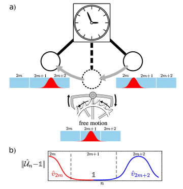
Figure 2: (a) Mechanical analogue of the time windows scheme (45). During the time between two successive ticks, the ends of the anchor (rigidly connected to the pendulum’s rod) don’t push on the teeth of the escape wheel and both pendulum and mechanism move freely. (b) Qualitative behaviour of the generator of the propagator (14) under the scheme (45). The action of the identity during the odd time windows causes the generator undergoes a smooth transition from $\hat{v}_{2m}$ to $\hat{v}_{2m+2}$. The colors correspond to the generator that is acting in the considered time. The shape of the curve depends on the shape of the pulse’s envelope.

Let us consider $W(i+1/2)-n^{\prime}\in[2mW,(2m+1)W]$, with $m\in\mathbb{N}$. In this case the pulse encompasses two time windows. According to (45) and considering the action of $\hat{N}_{\alpha}$ on the state of the clock, the generator reads

$$\frac{1}{W}\sum_{i} \hat{V}^{I}_{e}(s_{i})\otimes\hat{N}_{W(i+1/2)-n^{\prime}}=\alpha_{n^{\prime}}\hat{V}^{I}_{e}(s_{2m})+\beta_{n^{\prime}}\hat{V}^{I}_{e}(s_{2m+1})$$

$$=\alpha_{n^{\prime}}\hat{v}_{2m}+\beta_{n^{\prime}}\mathbb{1}\,,$$ (46)

where we define $\alpha_{n^{\prime}}=\frac{1}{W}\langle\hat{N}_{W(2m+1/2)-n^{\prime}}\rangle_{c}^{1/2}$ and $\beta_{n^{\prime}}=\frac{1}{W}\langle\hat{N}_{W(2m+1+1/2)-n^{\prime}}\rangle^{1/2}_{c}$. Thus in this case

$$\hat{\mathcal{U}}_{n^{\prime}} =\exp\{-i(\alpha_{n^{\prime}}\hat{v}_{2m}+\beta_{n^{\prime}}\mathbb{1})\Delta t\}$$

$$=\exp\{-i\alpha_{n^{\prime}}\hat{v}_{2m}\Delta t\}\exp\{-i\beta_{n^{\prime}}\mathbb{1}\Delta t\}$$

$$=\exp\{-i\alpha_{n^{\prime}}\hat{v}_{2m}\Delta t\}e^{-i\beta_{n^{\prime}}\Delta t}\,,$$ (47)

and the global phase factor can be neglected. At each $n^{\prime}$ the potential $\hat{v}_{2m}$ is weighted by the factor $\alpha_{n^{\prime}}$ that ranges between $0$ (the pulse is crossing another window) and a maximum that depends on the normalisation of the pulse (when the pulse is exactly centered on the $2m$th time window). This scheme allows us to approximate the action of the target time-dependent generator $V_{e}(t)$ on a mesh of time windows of size $W$. Nevertheless, a notable limitation is that each generator $V_{e}(s_{i})$ demands an effective time frame of $2W$ for execution. This, in conjunction with the modulation, imposes significant constraints on the accuracy of the achieved transformation. Notably, as $W$ increases, our discrete series offers a closer approximation to the continuous generator. Such trade-offs, that arise from the need to bridge the gap between continuous and discrete representations, are a common challenge in the realm of approximating continuous-time systems. Up to this point, we have not directly accounted for any clock degradation process. In the upcoming section, we explore the impact of clock degradation on the wave-packet dynamics, examining how the Hamiltonian in Eq. (9) affects also its shape. Understanding the underlying reasons for this degradation is crucial, given our reliance on the position of the particle in our time-keeping protocol.

References

- Cangemi et al. (2023) Loris Maria Cangemi, Chitrak Bhadra, and Amikam Levy, “Quantum engines and refrigerators,” (2023), arXiv:2302.00726 [quant-ph] .
- Aharonov and Bohm (1961) Y. Aharonov and D. Bohm, “Time in the quantum theory and the uncertainty relation for time and energy,” Phys. Rev. 122, 1649–1658 (1961).
- Woods et al. (2018) Mischa P. Woods, Ralph Silva, and Jonathan Oppenheim, “Autonomous quantum machines and finite-sized clocks,” Annales Henri Poincaré 20, 125–218 (2018).
- Woods and Horodecki (2023) Mischa P. Woods and Michał Horodecki, “Autonomous quantum devices: When are they realizable without additional thermodynamic costs?” Phys. Rev. X 13, 011016 (2023).
- Meier et al. (2024) Florian Meier, Marcus Huber, Paul Erker, and Jake Xuereb, “Autonomous quantum processing unit: What does it take to construct a self-contained model for quantum computation?” (2024), arXiv:2402.00111 [quant-ph] .
- Erker et al. (2017) Paul Erker, Mark T. Mitchison, Ralph Silva, Mischa P. Woods, Nicolas Brunner, and Marcus Huber, “Autonomous quantum clocks: Does thermodynamics limit our ability to measure time?” Phys. Rev. X 7, 031022 (2017).
- Xuereb et al. (2023) Jake Xuereb, Paul Erker, Florian Meier, Mark T. Mitchison, and Marcus Huber, “Impact of imperfect timekeeping on quantum control,” Physical Review Letters 131 (2023), 10.1103/physrevlett.131.160204.
- Feynman (2018) Richard P Feynman, “Simulating physics with computers,” in Feynman and computation (cRc Press, 2018) pp. 133–153.
- Feynman (1985) Richard P. Feynman, “Quantum mechanical computers,” Optics News 11, 11–20 (1985).
- Lloyd (1996) Seth Lloyd, “Universal quantum simulators,” Science 273, 1073–1078 (1996).
- Watkins et al. (2024) Jacob Watkins, Nathan Wiebe, Alessandro Roggero, and Dean Lee, “Time dependent hamiltonian simulation using discrete clock constructions,” (2024), arXiv:2203.11353 [quant-ph] .
- De Falco and Tamascelli (2004) Diego De Falco and Dario Tamascelli, “Quantum timing and synchronization problems,” International Journal of Modern Physics B 18, 623–631 (2004), https://doi.org/10.1142/S0217979204024240 .
- Woods (2024) Mischa P. Woods, “Quantum frequential computing: a quadratic run time advantage for all algorithms,” (2024), arXiv:2403.02389 [quant-ph] .
- Horodecki and Oppenheim (2013) Michał Horodecki and Jonathan Oppenheim, “Fundamental limitations for quantum and nanoscale thermodynamics,” Nature communications 4, 2059 (2013).
- Malabarba et al. (2015) Artur S L Malabarba, Anthony J Short, and Philipp Kammerlander, “Clock-driven quantum thermal engines,” New Journal of Physics 17, 045027 (2015).
- Pauli et al. (1980) Wolfgang Pauli, P. Achuthan, and K. Venkatesan, General Principles of Quantum Mechanics (Springer-Verlag, 1980) p. 63.
- Hilgevoord (2005) Jan Hilgevoord, “Time in quantum mechanics: a story of confusion,” Studies in History and Philosophy of Science Part B: Studies in History and Philosophy of Modern Physics 36, 29–60 (2005).
- Olkhovsky et al. (1974) VS Olkhovsky, E Recami, and AJ Gerasimchuk, “Time operator in quantum mechanics: I: Nonrelativistic case,” Il Nuovo Cimento A (1965-1970) 22, 263–278 (1974).
- Bauer (2014) Mariano Bauer, “A dynamical time operator in dirac’s relativistic quantum mechanics,” International Journal of Modern Physics A 29, 1450036 (2014).
- Leon and Maccone (2017) Juan Leon and Lorenzo Maccone, “The pauli objection,” Foundations of Physics 47, 1597–1608 (2017).
- Ciccarello (2018) Francesco Ciccarello, “Collision models in quantum optics,” Quantum Measurements and Quantum Metrology 4 (2018), 10.1515/qmetro-2017-0007.
- Gross et al. (2018) Jonathan A Gross, Carlton M Caves, Gerard J Milburn, and Joshua Combes, “Qubit models of weak continuous measurements: markovian conditional and open-system dynamics,” Quantum Science and Technology 3, 024005 (2018).
- Ciccarello et al. (2022) Francesco Ciccarello, Salvatore Lorenzo, Vittorio Giovannetti, and G. Massimo Palma, “Quantum collision models: Open system dynamics from repeated interactions,” Physics Reports 954, 1–70 (2022).
- Baragiola et al. (2012) Ben Q. Baragiola, Robert L. Cook, Agata M. Brańczyk, and Joshua Combes, “-photon wave packets interacting with an arbitrary quantum system,” Phys. Rev. A 86, 013811 (2012).
- Magnus (1954) Wilhelm Magnus, “On the exponential solution of differential equations for a linear operator,” Communications on pure and applied mathematics 7, 649–673 (1954).
- Diels and Rudolph (2006) Jean-Claude Diels and Wolfgang Rudolph, “1 - fundamentals,” in Ultrashort Laser Pulse Phenomena (Second Edition), edited by Jean-Claude Diels and Wolfgang Rudolph (Academic Press, Burlington, 2006) second edition ed., pp. 1–60.
- Berry and Balazs (1979) Michael V Berry and Nandor L Balazs, “Nonspreading wave packets,” American Journal of Physics 47, 264–267 (1979).
- Robertson (1929) H. P. Robertson, “The uncertainty principle,” Phys. Rev. 34, 163–164 (1929).
- Lan et al. (2013) Shau-Yu Lan, Pei-Chen Kuan, Brian Estey, Damon English, Justin M. Brown, Michael A. Hohensee, and Holger Müller, “A clock directly linking time to a particle’s mass,” Science 339, 554–557 (2013), https://www.science.org/doi/pdf/10.1126/science.1230767 .