Efficient Simulation of 1D Long-Range Interacting Systems at Any Temperature

Abstract

We introduce a method that ensures efficient computation of one-dimensional quantum systems with long-range interactions across all temperatures. Our algorithm operates within a quasi-polynomial runtime for inverse temperatures up to $\beta={\rm poly}(\ln(n))$. At the core of our approach is the Density Matrix Renormalization Group algorithm, which typically does not guarantee efficiency. We have created a new truncation scheme for the matrix product operator of the quantum Gibbs states, which allows us to control the error analytically. Additionally, our method is applied to simulate the time evolution of systems with long-range interactions, achieving significantly better precision than that offered by the Lieb-Robinson bound.

Introduction.— Unraveling the complex patterns of quantum many-body systems presents one of the most significant challenges in modern physics. Among these challenges, characterizing the thermal equilibrium quantum state (also known as the quantum Gibbs state) at zero and non-zero temperatures stands as a central target. These states are generally difficult to manage in high-dimensional systems as mentioned in previous studies [1, 2]. However, a variety of techniques have been developed to address their properties in one-dimensional systems [3, 4, 5, 6, 7, 8, 9, 10]. Notably, techniques such as the transfer matrix method used in classical Ising models [11] and its generalization to 1D quantum systems [12] have been well-recognized. More recently, the Density Matrix Renormalization Group (DMRG) algorithm has emerged as a promising approach [13, 14, 15, 16], enabling the numerical construction of the matrix product operator (MPO) that encapsulates all information about the equilibrium states [13, 16, 15, 17]. Despite its promise, providing a rigorous justification for the precision guarantee in the DMRG algorithm remains a critical open problem at both zero and non-zero temperatures [18, 7]. Nevertheless, several methods have been proposed to develop a ‘DMRG-type’ algorithm to construct the MPO with guaranteed accuracy and time efficiency [18, 7].

In one-dimensional systems at non-zero temperatures, the construction of the MPO for short-range interacting systems has received extensive attention. The pioneering method, based on the cluster expansion technique by Molnar et al. [4], introduced a polynomial-time algorithm. This algorithm works with a runtime scaling as $(n/\epsilon)^{\mathcal{O}(\beta)}$, where $n$ is the system size, to approximate the 1D quantum Gibbs state by the MPO within an error $\epsilon$. Subsequent advancements have refined the error bounds, with the leading-edge approach achieving a runtime of $e^{\tilde{\mathcal{O}}(\beta)+\tilde{\mathcal{O}}(\sqrt{\beta\ln(n/\epsilon)})}$ [7, 8]. This technique utilizes the imaginary-time adaptation of the Haah-Hastings-Kothari-Low (HHKL) decomposition, originally devised for real-time evolution [19].

Extending from the study of short-range interactions in one-dimensional (1D) systems, we explore the realm of long-range interactions, characterized by power-law decay. These interactions impart high-dimensional traits to systems, manifesting behaviors not observed in short-range interacting systems. Notably, phenomena such as phase transitions, typically associated with higher dimensions, can occur even in 1D systems with long-range interactions [20, 21, 22, 23, 24]. Additionally, long-range interactions are increasingly relevant in contemporary many-body physics experiments, such as those involving ultracold atomic systems [25, 26, 27, 28, 29, 30], highlighting their practical significance [31].

Beyond the realm of short-range interacting systems, the complexity analysis of long-range interactions presents substantial challenges, especially at low temperatures. Most existing methods are tailored specifically for short-range interactions, and their direct application to long-range systems often results in a loss of efficiency [32]. While the cluster expansion method proves effective at high temperatures [33, 34, 35], providing an efficient algorithm to analyze the properties of the quantum Gibbs state in systems with long-range interactions, it falls short at low temperatures. Notably, it does not offer an approximation by the MPO, leaving the computational approach at low temperatures as an unresolved issue.

In this letter, we introduce an efficiency-guaranteed method for constructing the MPO based on the DMRG algorithm. Our method achieves a runtime of:

$$e^{\mathcal{O}(\beta\ln^{3}(n/\epsilon))}\quad\text{(general cases)},$$ (1)

and for Hamiltonians that are $2$-local, as defined in Eq. (7) below, the runtime improves to:

$$e^{\tilde{\mathcal{O}}(\beta\ln^{2}(n/\epsilon))}\quad\text{(2-local cases)}.$$ (2)

These results demonstrate a quasi-polynomial time complexity under conditions where $\beta=\text{polylog}(n)$, a regime where the quantum Gibbs states typically approximate the non-critical ground state [36, 37]. Furthermore, while our primary focus has been on constructing MPOs for quantum Gibbs states, our approach is equally applicable to real-time evolutions. To our knowledge, this is the first rigorous justification of a classical simulation method with guaranteed efficiency for managing the real/imaginary-time dynamics of long-range interacting Hamiltonians.

In terms of technical advancements, the traditional DMRG algorithm faced challenges in accurately estimating the truncation errors of bond dimensions during iterative steps [14, 15] (see also Ref. [7, Sec. IV C therein]). To address this, we developed a new algorithm that captures the core mechanics, as illustrated in Fig. 1. Our approach comprises two main steps: (i) constructing the MPO at high temperatures with a precisely controlled error, using arbitrary Schatten $p$-norms, and (ii) merging high-temperature quantum Gibbs states into their low-temperature counterparts. The success of the first step allows us to apply techniques from Refs. [3, 7] in the second step. Hence, the primary challenge lies in the initial construction of the MPO. We begin by constructing the quantum Gibbs state in independent small blocks and iteratively merge them into larger ones. This approach retains the spirit of the original DMRG algorithm developed by White [13], focusing on local interactions and iterative improvements. A key innovation of our algorithm is the efficient control of the precision in the merging process, quantified by the general Schatten $p$-norm (see Proposition 2 below).

Setup.— We consider a one-dimensional quantum system composed of $n$ qudits, each in a $d$-dimensional Hilbert space. The total set of sites in this system is denoted by $\Lambda$, i.e., $\Lambda=\{1,2,3,\dots,n\}$. We define a $k$-local Hamiltonian $H$ for this system by:

$$H=\sum_{|Z|\leq k}h_{Z},\quad\max_{i\in\Lambda}\sum_{Z:Z\ni i}\|h_{Z}\|\leq g,$$ (3)

where $Z\subset\Lambda$, and $|Z|$ represents the cardinality of $Z$, meaning the number of sites involved in each interaction term $h_{Z}$. The term $\|\cdots\|$ denotes the operator norm, which is the maximum singular value of the operator. For any arbitrary subset $L\subseteq\Lambda$, the subset Hamiltonian $H_{L}$ is defined to include only those interaction terms involving sites in $L$, specifically:

$$H_{L}=\sum_{Z:Z\subset L}h_{Z}.$$

To elucidate the assumptions underpinning our analysis, let us consider a decomposition of the total system $\Lambda$ into subsets $A$ and $B$ such that $\Lambda=A\sqcup B$. Here, subset $A$ is defined as $[i,i^{\prime}]\cap\Lambda$ with $1\leq i<i^{\prime}\leq n$. We assume that the norm of the boundary interaction between $A$ and $B$, denoted by $\|\partial h_{A}\|$, is finite:

$$\|\partial h_{A}\|\leq\tilde{g},\quad\forall A,\quad\partial h_{A}:=H-(H_{A}+H_{B}),$$ (4)

where $\tilde{g}$ represents an $\mathcal{O}(1)$ constant. This condition is more general than the assumption of power-law decay of interactions. If we specifically consider the power-law decay condition in the form:

$$\sum_{Z:Z\ni\{i,i^{\prime}\}}\|h_{Z}\|\leq\frac{J}{|i-i^{\prime}|^{\alpha}}\quad\textrm{for}\quad i\neq i^{\prime},$$ (5)

then the condition in (4) is satisfied as long as $\alpha>2$ (see Supplementary materials [38]).

Throughout the paper, we analyze the quantum Gibbs state as follows:

$$\rho_{\beta}:=\frac{1}{Z_{\beta}}e^{-\beta H},\quad Z_{\beta}:=\operatorname{tr}\left(e^{-\beta H}\right).$$

We aim to approximate the Gibbs state $\rho_{\beta}$ by a MPO, which is generally described as follows:

$$M=\sum_{\begin{subarray}{c}s_{1},s_{2},\dots,s_{n}=1\\ s_{1}^{\prime},s_{2}^{\prime},\dots,s_{n}^{\prime}=1\end{subarray}}^{d} \operatorname{tr}\left(M_{1}^{[s_{1},s_{1}^{\prime}]}M_{2}^{[s_{2},s_{2}^{\prime}]}\cdots M_{n}^{[s_{n},s_{n}^{\prime}]}\right)$$

$$\left|s_{1},s_{2},\dots,s_{n}\right\rangle\left\langle s_{1}^{\prime},s_{2}^{\prime},\dots,s_{n}^{\prime}\right|,$$ (6)

where each $\{M_{j}^{[s_{j},s_{j}^{\prime}]}\}_{j,s_{j},s_{j}^{\prime}}$ is a $D\times D$ matrix, with $D$ referred to as the bond dimension. As measures of the approximation, we often use the Schatten $p$-norm as follows: $\left\|O\right\|_{p}:=[{\rm tr}(|O|^{p})]^{1/p}$ with $O$ an arbitrary operator and $|O|=\sqrt{O^{\dagger}O}$. For $p=1$, it is equivalent to the trace norm, and for $p=\infty$, it corresponds to the operator norm.

We denote the bond dimension of the MPO form of the Hamiltonian by $D_{H}$, which is at most of $n^{k}d^{k}$ in general [39]. In particular, if we restrict ourselves to a 2-local Hamiltonian in the form of:

$$H =\sum_{i<i^{\prime}}\frac{1}{|i-i^{\prime}|^{\alpha}}\sum_{\xi,\xi^{\prime}=1}^{d^{2}}J_{\xi,\xi^{\prime}}P_{i,\xi}\otimes P_{i^{\prime},\xi^{\prime}},$$ (7)

where $\{P_{i,\xi}\}_{\xi=1}^{d^{2}}$ denotes the operator bases at site $i$ and $J_{\xi,\xi^{\prime}}$ are the corresponding coefficients, the Hamiltonian can be approximated by an MPO with bond dimension $D_{H}=c_{H}\ln^{2}(n/\epsilon)$, where $c_{H}=\mathcal{O}(1)$, up to an error of $\epsilon$ (see Supplementary material [38, Lemma 2 therein]). We note that any subset Hamiltonian $H_{L}$ is also described by an MPO with the bond dimension $D_{H}$ of the global Hamiltonian.

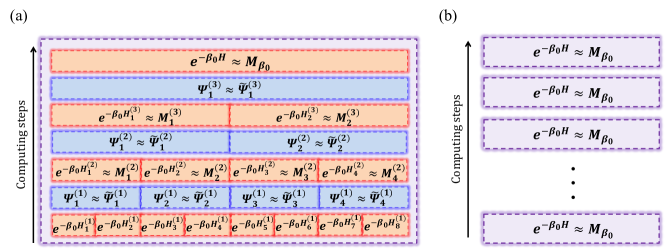
Figure 1: Illustration of the Matrix Product Operator (MPO) construction for approximating the quantum Gibbs state. (a) High-Temperature Quantum Gibbs States: The process begins with the product state of quantum Gibbs states across eight blocks. In the initial merging process $\{\Psi_{1}^{(1)},\Psi_{2}^{(1)},\Psi_{3}^{(1)},\Psi_{4}^{(1)}\}$, the block size is doubled, yielding quantum Gibbs states $\{e^{-\beta_{0}H_{1}^{(2)}},e^{-\beta_{0}H_{2}^{(2)}},e^{-\beta_{0}H_{3}^{(2)}},e^{-\beta_{0}H_{4}^{(2)}}\}$. After $q$ merging processes, with each process doubling the block size, the final block size becomes $2^{q}$ times the original. To cover the total system size $n$, $\log_{2}(n)$ merging processes are required. Each merging operator $\{\Psi_{s}^{(q)}\}_{s,q}$ is approximated by MPOs $\{\tilde{\Psi}_{s}^{(q)}\}_{s,q}$ with truncated bond dimensions [see Eq. (10)], facilitating the construction of the MPO $M_{\beta_{0}}$ for the high-temperature quantum Gibbs state $e^{-\beta_{0}H}$. Approximation errors are iteratively estimated as detailed in Proposition 2, noting that all approximation errors stem from these merging operators. (b) Low-Temperature Quantum Gibbs States: By iteratively combining high-temperature quantum Gibbs states, the Gibbs state at any desired temperature $\beta$ is achieved by exponentiating $e^{-\beta_{0}H}$ to $\beta/\beta_{0}$, where $\beta_{0}$ is chosen so that $\beta/\beta_{0}$ is an integer. The approximation error between $e^{-\beta H}$ and $(M_{\beta_{0}})^{\beta/\beta_{0}}$ is managed by controlling the error between $e^{-\beta_{0}H}$ and $M_{\beta_{0}}$ in terms of an arbitrary Schatten $p$-norm, as achieved in (13).

Main Result.— Our task is to develop a time-efficient method to approximate the quantum Gibbs state using an MPO with a fixed bond dimension. The main result concerning the time-efficient construction of the MPO is as follows:

Theorem. For an arbitrary $\beta$, we can efficiently compute the MPO $M_{\beta}$ that approximates the unnormalized Gibbs state up to an error $\epsilon$:

$$\left\|e^{-\beta H}-M_{\beta}\right\|_{p}\leq\epsilon\left\|e^{-\beta H}\right\|_{p},\quad\forall p.$$ (8)

The bond dimension of $M_{\beta}$ and the time complexity are given by $e^{C_{0}\beta\ln^{3}(n/\epsilon)}$, where $C_{0}$ is an $\mathcal{O}(1)$ constant. Typically, we consider $\epsilon=1/{\rm poly}(n)$, which leads to a time complexity of $e^{\mathcal{O}(\beta)\ln^{3}(n)}$. If we consider the 2-local Hamiltonian in Eq. (7), the time complexity qualitatively improves to $e^{C_{0}\ln^{2}(n/\epsilon)\ln\ln(n/\epsilon)}$. From the theorem, we can efficiently simulate the quantum Gibbs state in long-range interacting systems [40].

In the following, we detail the explicit calculation steps for constructing the MPO $M_{\beta}$, which is also illustrated in Fig. 1:

1. Initial State Preparation: We begin with a product state of the quantum Gibbs states of small blocks, each containing $2$ sites, at an inverse temperature $\beta_{0}$. This temperature $\beta_{0}$ is chosen to be smaller than $1/(24gk^{2})$. The exact MPO representation of the initial state has a bond dimension at most $d^{2}$, where $d$ is the dimension of the local Hilbert space.

2. Merging Operation: Adjacent quantum Gibbs states on blocks are merged using a merging operator $\Psi$. This operator is approximated by $\tilde{\Psi}$ using truncated expansions as described in Eq. (10), up to $m_{0}$-th order, where $m_{0}=\ln(n/\epsilon)$. Consequently, the bond dimension of the MPO form of $\tilde{\Psi}$ becomes $D_{H}^{\mathcal{O}(m_{0})}$, with $D_{H}$ representing the bond dimension of the Hamiltonian.

3. Approximation of High-Temperature Gibbs State: By repeating the merging processes $\log_{2}(n)$ times, we achieve the global quantum Gibbs state $e^{-\beta_{0}H}$. This high-temperature quantum Gibbs state is approximated by the MPO $M_{\beta_{0}}$, which has a bond dimension $D_{H}^{\mathcal{O}(m_{0}\ln(n))}$.

4. Approximation of Low-Temperature Gibbs State: The high-temperature quantum Gibbs state is connected $(\beta/\beta_{0})$ times to yield the MPO $(M_{\beta_{0}})^{\beta/\beta_{0}}$, serving as the approximation of the desired quantum Gibbs state $e^{-\beta H}$.

In the next section, we will focus on analytically estimating the precision error and the time complexity resulting from these approximations.

Finally, we discuss the preparation of quantum Gibbs states on a quantum computer. In conclusion, the time complexity (or circuit depth) for this preparation is also given by the quasi-polynomial form, i.e., $e^{C_{0}\beta\ln^{3}(n/\epsilon)}$. To achieve this, we first purify the Gibbs state into the form of a thermofield double state [41], which can also be well-approximated by a Matrix Product State (MPS) with the same bond dimension as that of $M_{\beta}$ [7, Sec. VI A therein]. For the quantum circuit representation of the MPS, we refer to Ref. [42, Appendix B therein], where it is generally shown that an arbitrary MPS with bond dimension $\chi$ can be constructed using a circuit with depth $n\times\mathrm{poly}(\chi)$. By setting $\chi=e^{C_{0}\beta\ln^{3}(n/\epsilon)}$ for the quantum Gibbs state’s preparation, we achieve the desired circuit depth.

Proof of main theorem.— We here provide the outline of the proof, and we defer the details to Supplementary materials [38]. We follow Steps 1 to 4 above and estimate the precision error depending on the bond dimension. We denote the Gibbs state of the block $L_{s}^{(q)}$ as $e^{-\beta_{0}H_{s}^{(q)}}$, where $H_{s}^{(q)}$ serves as an abbreviation for the subset Hamiltonian $H_{L_{s}^{(q)}}=\sum_{Z:Z\subset L_{s}^{(q)}}h_{Z}$ on block $L_{s}^{(q)}$. Under this notation, $e^{-\beta_{0}H_{1}^{(q_{0})}}=e^{-\beta_{0}H}$ represents the Gibbs state of the entire system, encompassing all interactions within the system.

We then estimate the error arising from the merging operations. In general, we define a merging operator $\Psi$ that connects two subsets, $A$ and $B$, as follows:

$$\Psi=e^{-\beta_{0}H_{AB}}e^{\beta_{0}(H_{A}+H_{B})},$$ (9)

which implies the relation $e^{-\beta_{0}H_{AB}}=\Psi e^{-\beta_{0}H_{A}}e^{-\beta_{0}H_{B}}$. Here, $\Psi$ facilitates the merging of the Gibbs states of $A$ and $B$ to form the combined Gibbs state on the larger block $AB$, as illustrated in Fig. 1(a). In this context, $H_{AB}=H_{A}+H_{B}+\partial h_{A}$, where $\partial h_{A}$ represents the boundary interactions between systems $A$ and $B$, as defined in Eq. (4).

To construct an MPO with a small bond dimension for $\Psi$, we first approximate $\Psi$ using a polynomial expansion in terms of $\beta_{0}$. However, the independent approximations of $e^{-\beta_{0}H_{AB}}$ and $e^{\beta_{0}(H_{A}+H_{B})}$ require polynomial degrees of at least $(\beta_{0}\left\|H_{AB}\right\|)^{1/2}$ and $(\beta_{0}\left\|H_{A}\right\|+\beta_{0}\left\|H_{B}\right\|)^{1/2}$, respectively [43]. This results in a demand for sub-exponentially large bond dimensions for an accurate approximation.

The key idea here is that by combining $e^{-\beta_{0}H_{AB}}$ and $e^{\beta_{0}(H_{A}+H_{B})}$ the truncation order is significantly reduced for a good approximation of $\Psi$. We adopt the following polynomial approximation of the merging operator (9):

$$\tilde{\Psi}=\sum^{m_{0}}_{m=0}\beta_{0}^{m}\sum_{s_{1}+s_{2}=m}(-1)^{s_{1}}\frac{H_{AB}^{s_{1}}(H_{A}+H_{B})^{s_{2}}}{s_{1}!s_{2}!},$$ (10)

where we apply the Taylor expansion for each of $e^{-\beta_{0}H_{AB}}$ and $e^{\beta_{0}(H_{A}+H_{B})}$ and truncate the terms with $\beta_{0}^{m}$ for $m>m_{0}$. Then, we prove the following precision error:
Proposition 1. If $\beta_{0}$ is smaller than $1/(24gk^{2})$, we achieve the approximation of

$$\|\Psi-\tilde{\Psi}\|\leq\delta_{0}\quad\textrm{for}\quad m_{0}\geq\log_{2}\left(c_{0}/\delta_{0}\right),$$ (11)

with $c_{0}=e^{\tilde{g}/(6gk^{2})}$ which is an $\mathcal{O}(1)$ constant.

To derive the MPO form of $\tilde{\Psi}$, we first create individual MPOs for each term in the expansion (10). These individual MPOs are then combined to obtain the MPO representation of $\tilde{\Psi}$. Given the MPO form of the Hamiltonians $H_{AB}$ and $H_{A}+H_{B}$, the bond dimension required for the term $H_{AB}^{s_{1}}(H_{A}+H_{B})^{s_{2}}$ is at most $D_{H}^{s_{1}}D_{H}^{s_{2}}=D_{H}^{m}$, where $s_{1}+s_{2}=m$. The total bond dimension required to represent all terms up to $m_{0}$ in the expansion is calculated as:

$$\sum_{m=0}^{m_{0}}(m+1)D_{H}^{m}\leq(m_{0}+1)^{2}D_{H}^{m_{0}}=:\tilde{D}_{\delta_{0}}.$$ (12)

Thus, we construct the MPO with the bond dimension $\tilde{D}_{\delta_{0}}$ to approximate the merging operator $\Psi$ for any arbitrary adjacent subsets $A$ and $B$.

After constructing the MPO approximation of the merging operator, we proceed to find the MPO for the combined Gibbs state. We in general consider the merging of $e^{-\beta_{0}H_{2s-1}^{(q-1)}}$ and $e^{-\beta_{0}H_{2s}^{(q-1)}}$, which is given by $e^{-\beta_{0}H_{s}^{(q)}}=\Psi_{s}^{(q-1)}e^{-\beta_{0}H_{2s-1}^{(q-1)}}e^{-\beta_{0}H_{2s}^{(q-1)}}$. Our purpose is to estimate the approximation by $\tilde{\Psi}_{s}^{(q-1)}M_{2s-1}^{(q-1)}M_{2s}^{(q-1)}$ when approximate MPOs $M_{2s-1}^{(q-1)}$ and $M_{2s}^{(q-1)}$ are given for $e^{-\beta_{0}H_{2s-1}^{(q-1)}}$ and $e^{-\beta_{0}H_{2s}^{(q-1)}}$, respectively. For simplicity, we denote $\Psi_{s}^{(q-1)}$ as $\Psi$ and $\tilde{\Psi}_{s}^{(q-1)}$ as $\tilde{\Psi}$, by omitting the indices $s$ and $q$.
Proposition 2. Let $M_{2s-1}^{(q-1)}$ and $M_{2s}^{(q-1)}$ represent the MPOs approximating $e^{-\beta_{0}H_{2s-1}^{(q-1)}}$ and $e^{-\beta_{0}H_{2s}^{(q-1)}}$, respectively, such that

$$\left\|e^{-\beta_{0}H_{i}^{(q-1)}}-M_{i}^{(q-1)}\right\|_{p}\leq\epsilon_{q-1}\left\|e^{-\beta_{0}H_{i}^{(q-1)}}\right\|_{p}$$

$\forall p$ with $i=2s-1,2s$. Using the approximate merging operator $\tilde{\Psi}$ with $\|\Psi-\tilde{\Psi}\|\leq\delta_{0}$, the merged quantum Gibbs state $e^{-\beta_{0}H_{s}^{(q)}}$ can be approximated as:

$$\left\|e^{-\beta_{0}H_{s}^{(q)}}-M_{s}^{(q)}\right\|_{p}\leq \epsilon_{q}\left\|e^{-\beta_{0}H_{s}^{(q)}}\right\|_{p},$$

with $\epsilon_{q}=a_{2}\delta_{0}+a_{1}\epsilon_{q-1}$, where the MPO $M_{s}^{(q)}$ is constructed as $M_{s}^{(q)}=\tilde{\Psi}M_{2s-1}^{(q-1)}M_{2s}^{(q-1)}$, and $a_{1}$ and $a_{2}$ are $\mathcal{O}(1)$ constants with $a_{1}>1$.

This shows that $\epsilon_{q}$ and $\epsilon_{q-1}$ are related by a linear equation, leading to a recursive relation on $q$. By solving this recursive relation, we find: $\epsilon_{q}\leq a_{2}\delta_{0}qa_{1}^{q-2},$ using the fact that $\epsilon_{1}=0$, because the MPO description of the initial state is exact. We then obtain the MPO approximation $M_{\beta_{0}}$ of the Gibbs state $e^{-\beta_{0}H}$, which results in the following error $\forall p$:

$$\left\|e^{-\beta_{0}H}-M_{\beta_{0}}\right\|_{p}\leq\epsilon^{\prime}_{0}\left\|e^{-\beta_{0}H}\right\|_{p}$$ (13)

with $\epsilon^{\prime}_{0}:=a_{2}\delta_{0}q_{0}a_{1}^{q_{0}-2}$. The MPO $M_{\beta_{0}}=M_{1}^{(q_{0})}$ is constructed through $q_{0}$ approximate merging processes $\tilde{\Psi}$, starting from the Gibbs states in layer 1. Consequently, the bond dimension increases by a factor of $\tilde{D}_{\delta_{0}}^{q_{0}}$, where $\tilde{D}_{\delta_{0}}$ was defined as the bond dimension of $\tilde{\Psi}$ in Eq. (12). If we consider the error $\|\Psi-\tilde{\Psi}\|\leq\delta_{0}=\epsilon/\mathrm{poly}(n)$, then the bond dimension becomes $\tilde{D}_{\delta_{0}}^{q_{0}}=D_{H}^{\mathcal{O}(\ln^{2}(n/\epsilon))}$, as $q_{0}=\log_{2}(n)$ and $\tilde{D}_{\delta_{0}}=D_{H}^{\mathcal{O}(\ln(1/\delta_{0}))}$.

Finally, we use the MPO $M_{\beta_{0}}$ for the high-temperature Gibbs state $e^{-\beta_{0}H}$ to approximate the target low-temperature Gibbs state $e^{-\beta H}$, as illustrated in Fig. 1(b). We combine the $(\beta/\beta_{0})$ MPOs $M_{\beta_{0}}$ to approximate the low-temperature Gibbs state, resulting in: $(M_{\beta_{0}})^{\beta/\beta_{0}}\approx e^{-\beta H}.$ Consequently, the bond dimension is multiplied $(\beta/\beta_{0})$ times, leading to a final required bond dimension of the order $D_{H}^{\mathcal{O}(\beta\ln^{2}(n/\epsilon))}$.

To derive the error bound, we use the inequality from [7, ineq. (C6) therein], which states the following: for fixed positive integers $p_{1}$ and $p_{2}$, if $\|e^{-\beta_{0}H}-M_{\beta_{0}}\|_{p_{1}p_{2}}\leq\epsilon^{\prime}\|e^{-\beta_{0}H}\|_{p_{1}p_{2}},$ then $\|e^{-p_{1}\beta_{0}H}-M_{\beta_{0}}^{p_{1}}\|_{p_{2}}\leq(3e/2)p_{1}\epsilon^{\prime}\|e^{-p_{1}\beta_{0}H}\|_{p_{2}}.$ We have already derived the MPO approximation for a general Schatten $p$-norm in (13). Therefore, we can obtain

$$\left\|e^{-\beta H}-(M_{\beta_{0}})^{\beta/\beta_{0}}\right\|_{p}\leq\epsilon_{\beta}\left\|e^{-\beta H}\right\|_{p},$$ (14)

where $\epsilon_{\beta}=5(\beta/\beta_{0})\epsilon^{\prime}_{0}.$ Since $a_{1}^{q_{0}}=\mathrm{poly}(n)$ with $q_{0}=\log_{2}(n)$, the choice of $\delta_{0}=\epsilon/\mathrm{poly}(n)$ yields the main precision bound in Eq. (8), where we defined $M_{\beta}=(M_{\beta_{0}})^{\beta/\beta_{0}}$ and assume $\beta<n$ without loss of generality [44].

By estimating each of the algorithm steps, we can see that the runtime is also upper-bounded by $D_{H}^{\mathcal{O}(\beta\ln^{2}(n/\epsilon))}$ (see Supplementary materials [38]). We thus prove the main theorem. $\square$

Extension to Real-Time Evolution– In our method, we did not rely on the fact that the inverse temperature $\beta$ is a real number. Therefore, it is possible to generalize our approach to cases where $\beta$ is a complex number. By considering the case where $\beta=it$, we can address the simulation of real-time evolution.

Given an MPO $M_{t}$ that approximates $e^{-iHt}$, we can estimate the error as: $\left\|e^{-iHt}\ket{\Psi}-M_{t}\ket{\Psi}\right\|\leq\left\|e^{-iHt}-M_{t}\right\|_{\infty}$ for an arbitrary quantum state $\ket{\Psi}$. By following our algorithm, we can construct an MPO $M_{t}$ for $e^{-iHt}$ that satisfies the error bound $\left\|e^{-iHt}-M_{t}\right\|_{\infty}\leq\epsilon\left\|e^{-iHt}\right\|_{\infty}=\epsilon$. The bond dimension and time complexity required are given by a quasi-polynomial form of $e^{\mathcal{O}(t\ln^{3}(n/\epsilon))}$. Compared to methods based on the Lieb-Robinson bound, our approach significantly reduces the time complexity. Assuming the Lieb-Robinson bound as $\left\|[O_{i}(t),O_{j}]\right\|\leq t^{\eta}/r^{\alpha}$ for $\alpha>2$ [45, 46, 47, 48], the time cost to calculate the average value of a time-evolved local observable $O_{i}(t)$ scales as $e^{(t^{\eta}/\epsilon)^{1/(\alpha-1)}}$.

Summary and outlook.— In this letter, we have presented an algorithm that achieves quasi-polynomial time complexity in approximating the quantum Gibbs state of 1D long-range interacting systems using MPOs. This was accomplished by adopting a DMRG-type method, as depicted in Fig. 1. We note that achieving quasi-polynomial complexity is likely the best attainable result in general [49]. However, there is hope to achieve polynomial time complexity for the $2$-local cases, as described in Eq. (7). Identifying the optimal time complexity for simulating long-range interacting systems remains an important open question.

Another intriguing avenue for exploration is whether our method can be extended to cases where the power-law decay is slower than $r^{-2}$ ($\alpha<2$), where the assumption of finite boundary interactions in Eq. (4) may no longer hold. In specific cases, this condition can still be recovered. For instance, in fermion systems with long-range hopping and short-range fermion-fermion interactions, the condition in Eq. (4) holds for $\alpha>3/2$ [50]. Another interesting class is the non-critical quantum Gibbs state, where power-law clustering is satisfied. In such systems, the MPO approximation is expected to hold for $\alpha>1$, since the mutual information for any bipartition obeys the area law [51].

S.I Several basic statements

S.I.1 Operator norm of the boundary interaction for long-range interacting systems when $\alpha>2$

We assume in the main text that the boundary interaction is bounded:

$$\left\|\partial h_{A}\right\|\leq\tilde{g},\qquad\forall A\subset\Lambda,$$ (S.1)

where the boundary interaction $\partial h_{A}$ is defined as the interaction acting on both subsystems $A$ and $B$, derived by subtracting the Hamiltonians $H_{A}$ and $H_{B}$, which act exclusively on $A$ and $B$, from the total Hamiltonian,

$$\partial h_{A}:=\sum_{Z:Z\cap A\neq\emptyset,Z\cap B\neq\emptyset}h_{Z}=H-(H_{A}+H_{B}).$$ (S.2)

We demonstrate that this assumption is inherently satisfied for long-range interactions with a power law decay of $\alpha>2$:

Lemma 1.

Considering the power-law decay of interactions in the form

$$\sum_{Z:Z\ni{i,i^{\prime}}}\left\|h_{Z}\right\|\leq\frac{J}{|i-i^{\prime}|^{\alpha}}\quad\textrm{for}\quad i\neq i^{\prime},$$ (S.3)

we prove that $\tilde{g}$ in Eq. (S.1) is $\mathcal{O}(1)$ as long as $\alpha>2$.

Proof of Lemma 1. Let us consider two adjacent subsystems, $A$ and $B$. From the definition of $\partial h_{A}$, we obtain

$$\left\|\partial h_{A}\right\| \leq\sum_{Z:Z\cap A\neq\emptyset,Z\cap B\neq\emptyset}\left\|h_{Z}\right\|\leq\sum_{i\in A}\sum_{i^{\prime}\in B}\sum_{Z:Z\ni i,i^{\prime}}\left\|h_{Z}\right\|\leq\sum_{i\in A}\sum_{i^{\prime}\in B}\frac{J}{|i-i^{\prime}|^{\alpha}}\leq\sum_{i=1}^{\infty}\sum_{j=1}^{\infty}\frac{J}{(i+j-1)^{\alpha}}=\zeta(\alpha-1),$$ (S.4)

where $\zeta(s)$ is the Riemann zeta function. For $\alpha>2$, we can choose $\tilde{g}=\zeta(\alpha-1)=\mathcal{O}(1)$. This completes the proof. $\square$

S.I.2 MPO approximation of the 2-local Hamiltonians

We generally obtain the MPO forms of $k$-local Hamiltonians which have the bond dimensions at most of $n^{k}d^{k}$. In this section, we show that the bond dimension is improved in the specific cases of the $2$-local Hamiltonians.

Lemma 2.

For a 2-local Hamiltonian of the form

$$H =\sum_{1\leq i<i^{\prime}\leq n}\frac{1}{|i-i^{\prime}|^{\alpha}}\sum_{\xi,\xi^{\prime}=1}^{d^{2}}J_{\xi,\xi^{\prime}}P_{i,\xi}\otimes P_{i^{\prime},\xi^{\prime}},$$ (S.5)

where $\{P_{i,\xi}\}_{\xi=1}^{d^{2}}$ are operator bases on site $i$ and $J_{\xi,\xi^{\prime}}$ are constants, there exists a Hamiltonian $\tilde{H}$ that approximates $H$ with an error bounded by $\left\|H-\tilde{H}\right\|\leq\epsilon_{H}$, and admits an MPO representation with bond dimension

$$D_{\tilde{H}}=c_{H}\ln^{2}(n/\epsilon_{H}),$$ (S.6)

where $c_{H}$ is an $\mathcal{O}(1)$ constant.

Remark. Here, the MPO form for the Hamiltonian $\tilde{H}$ is not exactly the same as that of the original Hamiltonian $H$. We hence need to take into account the error between $H$ and $\tilde{H}$ for the simulation of the quantum Gibbs states (see Sec. S.II.5).

Proof of Lemma 2. We approximate $r^{-\alpha}$ as an exponential series in accordance with Ref. [52, Theorem 3], as follows:

$$\left|r^{-\alpha}-\sum_{s\in\mathbb{Z}}e^{\alpha sx}e^{-e^{sx}r}\right|\leq\epsilon\quad\textrm{for}\quad r\geq 1,$$

$$x=\frac{2\pi}{\ln(3)+\alpha\ln[1/\cos(1)]+\ln(1/\epsilon)}.$$ (S.7)

We then consider the finite truncation as $s\in\mathbb{Z}_{m}=[-m,m]$. We obtain

$$\left|\sum_{s\in\mathbb{Z}}e^{\alpha sx}e^{-e^{sx}r}-\sum_{s\in\mathbb{Z}_{m}}e^{\alpha sx}e^{-e^{sx}r}\right|\leq\sum_{s<-m}e^{\alpha sx}+\sum_{s>m}e^{\alpha sx-e^{sx}}.$$ (S.8)

We assume that $m$ satisfies

$$\alpha mx-e^{mx}\leq-\alpha mx\quad\longrightarrow\quad e^{mx}\geq 2\alpha mx\quad \longrightarrow\quad mx\geq-{\rm ProductLog}\left(-\frac{1}{2\alpha}\right)$$

$$\longrightarrow\quad m\geq\frac{2}{x}\ln(2\alpha),$$ (S.9)

where ${\rm ProductLog}(x)$ is equivalent to the Lambert W function $W(x)$, defined by $x=W(x)e^{W(x)}$.

Under the assumption, we reduce the inequality (S.8) to

$$\left|\sum_{s\in\mathbb{Z}}e^{\alpha sx}e^{-e^{sx}r}-\sum_{s\in\mathbb{Z}_{m}}e^{\alpha sx}e^{-e^{sx}r}\right|\leq 2\sum_{s>m}e^{-\alpha sx}=\frac{2e^{-\alpha xm}}{e^{\alpha x}-1}=\frac{2}{e^{\alpha x}-1}\left(\frac{\epsilon}{2\alpha}\right)^{2\alpha}$$ (S.10)

with

$$m=\left\lceil\frac{2}{x}\ln(2\alpha/\epsilon)\right\rceil.$$ (S.11)

Under the above choice, we obtain

$$\left|r^{-\alpha}-\sum_{s\in\mathbb{Z}_{m}}e^{\alpha sx}e^{-e^{sx}r}\right|\leq\epsilon+\frac{2}{e^{\alpha x}-1}\left(\frac{\epsilon}{2\alpha}\right)^{2\alpha}\leq\zeta\epsilon,$$ (S.12)

where $\zeta$ is an $\mathcal{O}(1)$ constant for $\alpha\geq 2$.

Based on this approximation, we define the Hamiltonian $\tilde{H}$ as:

$$\tilde{H} =\sum_{1\leq i<i^{\prime}\leq n}\sum_{s\in\mathbb{Z}_{m}}e^{\alpha sx}e^{-e^{sx}|i-i^{\prime}|}\sum_{\xi,\xi^{\prime}=1}^{d^{2}}J_{\xi,\xi^{\prime}}P_{i,\xi}\otimes P_{i^{\prime},\xi^{\prime}}.$$ (S.13)

We then obtain

$$\left\|H-\tilde{H}\right\|\leq\zeta\epsilon\sum_{1\leq i<i^{\prime}\leq n}\sum_{\xi,\xi^{\prime}=1}^{d^{2}}J_{\xi,\xi^{\prime}}\left\|P_{i,\xi}\otimes P_{i^{\prime},\xi^{\prime}}\right\|\leq\bar{J}n^{2}\zeta\epsilon,$$ (S.14)

with

$$\bar{J}:=\sum_{\xi,\xi^{\prime}=1}^{d^{2}}|J_{\xi,\xi^{\prime}}|,$$ (S.15)

where we set the operator bases such that $\left\|P_{i,\xi}\right\|=1$ for $\forall i$ and $\forall\xi$.

To ensure an approximation error of $\epsilon_{H}$ for $\left\|H-\tilde{H}\right\|$, we let $\bar{J}n^{2}\zeta\epsilon=\epsilon_{H}$ (or $\epsilon=\epsilon_{H}/(\bar{J}\zeta n^{2})$), which implies

$$m=\left\lceil\frac{2}{x}\ln(2\alpha/\epsilon)\right\rceil\leq c^{\prime}_{H}\ln^{2}(n/\epsilon_{H}),$$ (S.16)

where $c^{\prime}_{H}$ is a constant of order $\mathcal{O}(1)$.

Moreover, it has been shown that each Hamiltonian of the form $\sum_{1\leq i<i^{\prime}\leq n}e^{\alpha sx}e^{-e^{sx}|i-i^{\prime}|}\sum_{\xi,\xi^{\prime}=1}^{d^{2}}J_{\xi,\xi^{\prime}}P_{i,\xi}\otimes P_{i^{\prime},\xi^{\prime}}$ with exponential decay admits an MPO representation with a bond dimension of $\mathcal{O}(d^{2})$ [53]. Therefore, the MPO representation of $\tilde{H}$ can be constructed by combining the MPOs of each term, resulting in a total bond dimension of:

$$D_{\tilde{H}} =c_{H}\ln^{2}(n/\epsilon_{H})$$ (S.17)

for $d=\mathcal{O}(1)$, where $c_{H}$ is an $\mathcal{O}(1)$ constant. This completes the proof. $\square$

S.II Proof of main propositions and technical details

S.II.1 Proof of Proposition 1 in the main text

We now present the proof of Proposition 1 in the main text. For the convenience of readers, we recall the setup. We define a merging operator $\Psi$ that connects two subsets $A$ and $B$ as follows:

$$\Psi=e^{-\beta_{0}H_{AB}}e^{\beta_{0}(H_{A}+H_{B})},\qquad H_{AB}=H_{A}+H_{B}+\partial h_{A},$$ (S.18)

which leads to the relation

$$e^{-\beta_{0}H_{AB}}=\Psi\,e^{-\beta_{0}H_{A}}e^{-\beta_{0}H_{B}}.$$ (S.19)

Proposition 1.

Consider the polynomial expansion of the merging operator $\Psi$ in powers of $\beta_{0}$, given by:

$$\Psi=e^{-\beta_{0}H_{AB}}e^{\beta_{0}(H_{A}+H_{B})} =e^{-\beta_{0}H_{AB}}e^{\beta_{0}(H_{AB}-\partial h_{A})}$$

$$=\sum_{m=0}^{\infty}\beta_{0}^{m}\sum_{s_{1}+s_{2}=m}\frac{1}{s_{1}!s_{2}!}(-H_{AB})^{s_{1}}(H_{AB}-\partial h_{A})^{s_{2}}.$$ (S.20)

We truncate the above series to $m_{0}$ terms and denote the resulting truncated series as $\tilde{\Psi}$:

$$\tilde{\Psi} =\sum_{m=0}^{m_{0}}\beta_{0}^{m}\sum_{s_{1}+s_{2}=m}\frac{1}{s_{1}!s_{2}!}(-H_{AB})^{s_{1}}(H_{AB}-\partial h_{A})^{s_{2}}.$$ (S.21)

Then, if $\beta_{0}$ is smaller than $\frac{1}{24gk^{2}}$, we achieve the approximation

$$\left\|\Psi-\tilde{\Psi}\right\|\leq\delta_{0}\quad\textrm{for}\quad m_{0}\geq\log_{2}\left(\frac{c_{0}}{\delta_{0}}\right),$$ (S.22)

where $c_{0}=e^{\tilde{g}/(6gk^{2})}$ is a constant of $\mathcal{O}(1)$.

Proof of Proposition 1. We derive the approximation of the truncation of the expansion. To this end, we first reformulate each term in the expansion (S.20) by employing an alternative expansion, specifically using the interaction picture:

$$e^{\beta_{0}(H_{AB}-\partial h_{A})}=e^{\beta_{0}H_{AB}}\mathcal{T}\left(e^{-\int_{0}^{\beta_{0}}\partial h_{x}\,dx}\right),$$ (S.23)

where we define $\partial h_{x}:=e^{-xH_{AB}}\partial h_{A}e^{xH_{AB}}$ and $\mathcal{T}$ is the time-ordering operator. We then obtain

$$\Psi =e^{-\beta_{0}H_{AB}}e^{\beta_{0}(H_{AB}-\partial h_{A})}$$

$$=\mathcal{T}\left(e^{-\int_{0}^{\beta_{0}}\partial h_{x}\,dx}\right)=\sum_{s=0}^{\infty}(-1)^{s}\int_{0}^{\beta_{0}}dx_{1}\int_{0}^{x_{1}}dx_{2}\cdots\int_{0}^{x_{s-1}}dx_{s}\,\partial h_{x_{1}}\partial h_{x_{2}}\cdots\partial h_{x_{s}}.$$ (S.24)

By applying the decomposition

$$\partial h_{x}=\sum_{p=0}^{\infty}\frac{(-x)^{p}}{p!}\mathrm{ad}_{H_{AB}}^{p}(\partial h_{A})=:\sum_{p=0}^{\infty}\frac{(-x)^{p}}{p!}\partial h^{(p)},$$ (S.25)

the $m$-th order term in the expansion of $\Psi$ in powers of $\beta_{0}$, which includes the contribution from $\beta_{0}^{m}$ in Eq. (S.24), is expressed as

$$\Psi_{0} :=1,$$ (S.26)

$$\Psi_{m} :=\sum_{s=1}^{m}\sum_{p_{1}+p_{2}+\cdots+p_{s}=m-s}(-1)^{s}\int_{0}^{\beta_{0}}dx_{1}\int_{0}^{x_{1}}dx_{2}\cdots\int_{0}^{x_{s-1}}dx_{s}\,\frac{(-x_{1})^{p_{1}}}{p_{1}!}\cdots\frac{(-x_{s})^{p_{s}}}{p_{s}!}\,\partial h^{(p_{1})}\cdots\partial h^{(p_{s})}$$ (S.27)

for $\forall m\geq 1$. As both Eq. (S.20) and Eq. (S.24) are expansions in powers of $\beta_{0}$, the term $\Psi_{m}$ defined above corresponds to the $m$th order term in Eq. (S.20):

$$\Psi_{m}=\beta_{0}^{m}\sum_{s_{1}+s_{2}=m}\frac{1}{s_{1}!s_{2}!}(-H_{AB})^{s_{1}}(H_{AB}-\partial h_{A})^{s_{2}},$$ (S.28)

which we aim to upper-bound.

The norm of $\Psi_{m}$ is upper-bounded as

$$\|\Psi_{m}\| \leq\sum_{s=1}^{m}\beta_{0}^{m-s}\sum_{p_{1}+p_{2}+\cdots+p_{s}=m-s}\int_{0}^{\beta_{0}}dx_{1}\,\int_{0}^{x_{1}}dx_{2}\cdots\int_{0}^{x_{s-1}}dx_{s}\,\prod_{j=1}^{s}\frac{1}{p_{j}!}\|\partial h^{(p_{j})}\|$$

$$\leq\beta_{0}^{m}\sum_{s=1}^{m}\frac{1}{s!}\sum_{p_{1}+p_{2}+\cdots+p_{s}=m-s}\prod_{j=1}^{s}\frac{1}{p_{j}!}\|\partial h^{(p_{j})}\|.$$ (S.29)

From Theorem 2.1 in [54], if $H$ is a $k$-local and $g$-extensive Hamiltonian and $A$ is a $r$-local operator, then

$$\left\|[H,A]\right\|\leq 6gkr\|A\|.$$ (S.30)

Since $H_{AB}$ and $\partial h_{A}$ are $k$-local Hamiltonians, $\text{ad}_{H_{AB}}^{p-1}(\partial h_{A})$ is at most $kp$-local. Using the inequality (S.30), we get

$$\|\partial h^{(p)}\|=\|\text{ad}_{H_{AB}}^{p}(\partial h_{A})\| \leq 6gk(kp)\|\text{ad}_{H_{AB}}^{p-1}(\partial h_{A})\|.$$ (S.31)

By iterating the above process for $\|\text{ad}_{H_{AB}}^{p^{\prime}}(\partial h_{A})\|$ with $p^{\prime}\leq p-2$ and using (S.1), we obtain

$$\|\partial h^{(p)}\|\leq(6gk^{2})^{p}p!\tilde{g}=:C^{p}p!\tilde{g},$$ (S.32)

where we define $C:=6gk^{2}$. Substituting Eq. (S.32) into Eq. (S.29), we get

$$\|\Psi_{m}\| \leq\beta_{0}^{m}\sum_{s=1}^{m}\frac{C^{m-s}\tilde{g}^{s}}{s!}\sum_{p_{1}+p_{2}+\cdots+p_{s}=m-s}1=\beta_{0}^{m}\sum_{s=1}^{m}\frac{C^{m-s}\tilde{g}^{s}}{s!}\left(\binom{m-s}{s}\right).$$ (S.33)

Using $\left(\binom{m-s}{s}\right)=\binom{m-1}{s}\leq 2^{m}$ ,

$$\|\Psi_{m}\| \leq(2C\beta_{0})^{m}\sum_{s=1}^{m}\frac{1}{s!}\left(\frac{\tilde{g}}{C}\right)^{s}\leq(2C\beta_{0})^{m}e^{\tilde{g}/C}.$$ (S.34)

Given the assumption $\beta_{0}\leq\frac{1}{24gk^{2}}=\frac{1}{4C}$, it follows that

$$\|\Psi_{m}\|\leq 2^{-m}e^{\tilde{g}/C},$$ (S.35)

which exhibits exponential decay with respect to $m$. Thus, the truncation error resulting from approximating $\Psi$ by $\tilde{\Psi}$ is bounded by

$$\left\|\Psi-\tilde{\Psi}\right\|\leq\sum_{m=m_{0}+1}^{\infty}\left\|\Psi_{m}\right\|\leq\sum_{m=m_{0}+1}^{\infty}2^{-m}e^{\tilde{g}/C}=e^{\tilde{g}/C}2^{-m_{0}}.$$ (S.36)

Letting $c_{0}=e^{\tilde{g}/C}=e^{\tilde{g}/(6gk^{2})}$, to achieve the desired error $\|\Psi-\tilde{\Psi}\|\leq\delta_{0}$, it is sufficient to choose $m_{0}$ such that $\|\Psi-\tilde{\Psi}\|\leq c_{0}2^{-m_{0}}\leq\delta_{0}$, i.e.,

$$m_{0}\geq\log_{2}\left(\frac{c_{0}}{\delta_{0}}\right).$$ (S.37)

This completes the proof of Proposition 1. $\square$

S.II.2 Proof of Proposition 2 in the main text

In this subsection, we prove Proposition 2 in the main text, which concerns the approximation of the merged quantum Gibbs state.

Proposition 2.

Let $M_{2s-1}^{(q-1)}$ and $M_{2s}^{(q-1)}$ represent the MPOs approximating $e^{-\beta_{0}H_{2s-1}^{(q-1)}}$ and $e^{-\beta_{0}H_{2s}^{(q-1)}}$, respectively, such that

$$\left\|e^{-\beta_{0}H_{2s-1}^{(q-1)}}-M_{2s-1}^{(q-1)}\right\|_{p} \leq\epsilon_{q-1}\left\|e^{-\beta_{0}H_{2s-1}^{(q-1)}}\right\|_{p},$$ (S.38)

$$\left\|e^{-\beta_{0}H_{2s}^{(q-1)}}-M_{2s}^{(q-1)}\right\|_{p} \leq\epsilon_{q-1}\left\|e^{-\beta_{0}H_{2s}^{(q-1)}}\right\|_{p},$$ (S.39)

for an arbitrary Schatten $p$-norm. Using the merging operator $\tilde{\Psi}_{s}^{(q-1)}$, which provides an approximation to $\Psi_{s}^{(q-1)}$ with the error bounded by $\|\Psi_{s}^{(q-1)}-\tilde{\Psi}_{s}^{(q-1)}\|\leq\delta_{0}$, the merged quantum Gibbs state $e^{-\beta_{0}H_{s}^{(q)}}$ can be approximated by the newly constructed MPO $M_{s}^{(q)}$ based on $M_{s}^{(q)}=\tilde{\Psi}_{s}^{(q-1)}M_{2s-1}^{(q-1)}M_{2s}^{(q-1)}$ as

$$\left\|e^{-\beta_{0}H_{s}^{(q)}}-M_{s}^{(q)}\right\|_{p}\leq\epsilon_{q}\left\|e^{-\beta_{0}H_{s}^{(q)}}\right\|_{p},$$ (S.40)

with the error

$$\epsilon_{q}=a_{2}\delta_{0}+a_{1}\epsilon_{q-1}.$$ (S.41)

Here, $a_{1}$ and $a_{2}$ are $\mathcal{O}(1)$ constants with $a_{1}>1$, defined as

$$a_{1} :=12e^{\tilde{g}/(4gk^{2})},\qquad a_{2}:=2e^{\tilde{g}/(24gk^{2})}.$$ (S.42)

Proof of Proposition 2. The merging operator is defined as $\Psi_{s}^{(q-1)}=e^{-\beta_{0}H_{s}^{(q)}}e^{\beta_{0}(H_{2s-1}^{(q-1)}+H_{2s}^{(q-1)})}$, and the approximate merging operator $\tilde{\Psi}_{s}^{(q-1)}$ is given by Eq. (S.21). With the MPO defined as $M_{s}^{(q)}=\tilde{\Psi}_{s}^{(q-1)}M_{2s-1}^{(q-1)}M_{2s}^{(q-1)}$, we proceed with the following inequality:

$$\left\|e^{-\beta_{0}H_{s}^{(q)}}-M_{s}^{(q)}\right\|_{p} =\left\|\Psi_{s}^{(q-1)}e^{-\beta_{0}H_{2s-1}^{(q-1)}}e^{-\beta_{0}H_{2s}^{(q-1)}}-\tilde{\Psi}_{s}^{(q-1)}M_{2s-1}^{(q-1)}M_{2s}^{(q-1)}\right\|_{p}$$

$$\leq\left\|\left(\Psi_{s}^{(q-1)}-\tilde{\Psi}_{s}^{(q-1)}\right)e^{-\beta_{0}H_{2s-1}^{(q-1)}}e^{-\beta_{0}H_{2s}^{(q-1)}}\right\|_{p}$$

$$\qquad+\left\|\tilde{\Psi}_{s}^{(q-1)}\left(e^{-\beta_{0}H_{2s-1}^{(q-1)}}e^{-\beta_{0}H_{2s}^{(q-1)}}-M_{2s-1}^{(q-1)}M_{2s}^{(q-1)}\right)\right\|_{p}$$

$$\leq\left\|\Psi_{s}^{(q-1)}-\tilde{\Psi}_{s}^{(q-1)}\right\|_{\infty}\left\|e^{-\beta_{0}H_{2s-1}^{(q-1)}}e^{-\beta_{0}H_{2s}^{(q-1)}}\right\|_{p}$$

$$\qquad+\left\|\tilde{\Psi}_{s}^{(q-1)}\right\|_{\infty}\left\|e^{-\beta_{0}H_{2s-1}^{(q-1)}}e^{-\beta_{0}H_{2s}^{(q-1)}}-M_{2s-1}^{(q-1)}M_{2s}^{(q-1)}\right\|_{p}.$$ (S.43)

From Ref. [55, Lemma 7 therein], we can prove for arbitrary operators ${\mathcal{A}}$ and ${\mathcal{B}}$

$$\left\|e^{{\mathcal{A}}+{\mathcal{B}}}-e^{{\mathcal{A}}}\right\|_{p}\leq e^{\left\|{\mathcal{B}}\right\|}\left\|{\mathcal{B}}\right\|\left\|e^{{\mathcal{A}}}\right\|_{p}.$$ (S.44)

By applying the inequality and substituting $-\beta_{0}H_{s}^{(q)}$ for ${\mathcal{A}}$ and $\beta_{0}H_{s}^{(q)}-\beta_{0}H_{2s}^{(q-1)}-\beta_{0}H_{2s-1}^{(q-1)}$ for ${\mathcal{B}}$, we obtain $\left\|{\mathcal{B}}\right\|\leq\tilde{g}$ from assumption (S.1) and

$$\left\|e^{-\beta_{0}H_{2s-1}^{(q-1)}}e^{-\beta_{0}H_{2s}^{(q-1)}}-e^{-\beta_{0}H_{s}^{(q)}}\right\|_{p}\leq e^{\beta_{0}\tilde{g}}\left\|e^{-\beta_{0}H_{s}^{(q)}}\right\|_{p}.$$ (S.45)

The triangle inequality leads to

$$\left\|e^{-\beta_{0}H_{2s-1}^{(q-1)}}e^{-\beta_{0}H_{2s}^{(q-1)}}\right\|_{p}\leq\left(e^{\beta_{0}\tilde{g}}+1\right)\left\|e^{-\beta_{0}H_{s}^{(q)}}\right\|_{p}\leq 2e^{\beta_{0}\tilde{g}}\left\|e^{-\beta_{0}H_{s}^{(q)}}\right\|_{p}.$$ (S.46)

From the above inequality and the condition $\|\Psi_{s}^{(q-1)}-\tilde{\Psi}_{s}^{(q-1)}\|_{p}\leq\delta_{0}$, we reduce inequality (S.43) to

$$\left\|e^{-\beta_{0}H_{s}^{(q)}}-M_{s}^{(q)}\right\|_{p} \leq 2\delta_{0}e^{\beta_{0}\tilde{g}}\left\|e^{-\beta_{0}H_{s}^{(q)}}\right\|_{p}+\left\|\tilde{\Psi}_{s}^{(q-1)}\right\|_{\infty}\left\|e^{-\beta_{0}H_{2s-1}^{(q-1)}}e^{-\beta_{0}H_{2s}^{(q-1)}}-M_{2s-1}^{(q-1)}M_{2s}^{(q-1)}\right\|_{p}.$$ (S.47)

To estimate the second term on the RHS of (S.47), we use the following mathematical lemma:

Lemma 3.

If two operators $O_{1}$ and $O_{2}$ act on disjoint supports, with their respective approximations $\tilde{O}_{1}$ and $\tilde{O}_{2}$ defined on the supports of $O_{1}$ and $O_{2}$, satisfying

$$\left\|O_{1}-\tilde{O}_{1}\right\|_{p} \leq\epsilon\left\|O_{1}\right\|_{p},$$ (S.48)

$$\left\|O_{2}-\tilde{O}_{2}\right\|_{p} \leq\epsilon\left\|O_{2}\right\|_{p},$$ (S.49)

with $\epsilon<1$, we then obtain

$$\left\|O_{1}O_{2}-\tilde{O}_{1}\tilde{O}_{2}\right\|_{p}\leq 3\epsilon\left\|O_{1}O_{2}\right\|_{p}.$$ (S.50)

Proof of Lemma 3. When $O_{1}$ and $O_{2}$ operate on disjoint supports, we have $\left\|O_{1}O_{2}\right\|_{p}=\left\|O_{1}\right\|_{p}\left\|O_{2}\right\|_{p}$. By leveraging this fact along with Eqs. (S.48) and (S.49), we derive

$$\left\|O_{1}O_{2}-\tilde{O}_{1}\tilde{O}_{2}\right\|_{p} \leq\left\|O_{1}(O_{2}-\tilde{O}_{2})\right\|_{p}+\left\|(O_{1}-\tilde{O}_{1})\tilde{O}_{2}\right\|_{p}$$

$$=\left\|O_{1}\right\|_{p}\left\|O_{2}-\tilde{O}_{2}\right\|_{p}+\left\|O_{1}-\tilde{O}_{1}\right\|_{p}\left\|\tilde{O}_{2}\right\|_{p}$$

$$\leq\epsilon\left\|O_{1}\right\|_{p}\left\|O_{2}\right\|_{p}+\epsilon\left\|O_{1}\right\|_{p}\left\|\tilde{O}_{2}\right\|_{p}.$$

The relation $\left\|\tilde{O}_{2}\right\|_{p}\leq\left\|O_{2}\right\|_{p}+\left\|O_{2}-\tilde{O}_{2}\right\|_{p}\leq(1+\epsilon)\left\|O_{2}\right\|_{p}$ and $\epsilon^{2}\leq\epsilon$ leads to

$$\left\|O_{1}O_{2}-\tilde{O}_{1}\tilde{O}_{2}\right\|_{p} \leq\epsilon\left\|O_{1}\right\|_{p}\left\|O_{2}\right\|_{p}+\epsilon(1+\epsilon)\left\|O_{1}\right\|_{p}\left\|O_{2}\right\|_{p}=(2\epsilon+\epsilon^{2})\left\|O_{1}\right\|_{p}\left\|O_{2}\right\|_{p}\leq 3\epsilon\left\|O_{1}\right\|_{p}\left\|O_{2}\right\|_{p}.$$

This completes the proof of Lemma 3. $\square$

Since $e^{-\beta_{0}H_{2s-1}^{(q-1)}}$ and $e^{-\beta_{0}H_{2s}^{(q-1)}}$ act on disjoint supports (i.e., $L_{2s-1}^{(q-1)}\cap L_{2s}^{(q-1)}=\emptyset$), applying the Lemma 3 yields:

$$\left\|e^{-\beta_{0}H_{2s-1}^{(q-1)}}e^{-\beta_{0}H_{2s}^{(q-1)}}-M_{2s-1}^{(q-1)}M_{2s}^{(q-1)}\right\|_{p} \leq 3\epsilon_{q-1}\left\|e^{-\beta_{0}H_{2s-1}^{(q-1)}}e^{-\beta_{0}H_{2s}^{(q-1)}}\right\|_{p}$$

$$\leq 6\epsilon_{q-1}e^{\beta_{0}\tilde{g}}\left\|e^{-\beta_{0}H_{s}^{(q)}}\right\|_{p},$$ (S.51)

where we use the upper bound (S.46) in the second inequality.

We then upper-bound the norm of $\tilde{\Psi}_{s}^{(q-1)}$, which is the truncated series up to $m_{0}$ terms in the expansion of $\Psi_{s}^{(q-1)}$ as in Eq. (S.21). By using the upper bound (S.35), which gives $\|\Psi_{m}\|\leq 2^{-m}e^{\tilde{g}/C}$, we obtain

$$\left\|\tilde{\Psi}_{s}^{(q-1)}\right\|\leq\sum_{m=0}^{m_{0}}\left\|\Psi_{m}\right\|\leq\sum_{m=0}^{m_{0}}2^{-m}e^{\tilde{g}/C}\leq 2e^{\tilde{g}/C}=2e^{\tilde{g}/(6gk^{2})}.$$ (S.52)

We thus derive the upper bound

$$\left\|\tilde{\Psi}_{s}^{(q-1)}\right\|_{\infty}\left\|e^{-\beta_{0}H_{2s-1}^{(q-1)}}e^{-\beta_{0}H_{2s}^{(q-1)}}-M_{2s-1}^{(q-1)}M_{2s}^{(q-1)}\right\|_{p}\leq 12e^{\tilde{g}/(6gk^{2})+\beta_{0}\tilde{g}}\epsilon_{q-1}\left\|e^{-\beta_{0}H_{s}^{(q)}}\right\|_{p}.$$ (S.53)

By combining the above inequality with (S.47), we have

$$\left\|e^{-\beta_{0}H_{s}^{(q)}}-M_{s}^{(q)}\right\|_{p} \leq\left(2\delta_{0}e^{\beta_{0}\tilde{g}}+12e^{\tilde{g}/(6gk^{2})+\beta_{0}\tilde{g}}\epsilon_{q-1}\right)\left\|e^{-\beta_{0}H_{s}^{(q)}}\right\|_{p}$$

$$\leq\left(2\delta_{0}e^{\tilde{g}/(24gk^{2})}+12e^{\tilde{g}/(4gk^{2})}\epsilon_{q-1}\right)\left\|e^{-\beta_{0}H_{s}^{(q)}}\right\|_{p},$$ (S.54)

where we use $\beta_{0}\leq 1/(24gk^{2})$. Thus, we establish the desired inequality (S.40), along with Eqs. (S.41) and (S.42). This completes the proof of Proposition 2. $\square$

S.II.3 Explicit estimation of the bond dimension

From Proposition 2, we see that $\epsilon_{q}$ follows a recursive relation, with $\epsilon_{1}=0$ since the blocks in layer 1 have exact MPOs. Using $\epsilon_{1}=0$, the recursive relation yields the following relations:

$$\epsilon_{q} =a_{2}\delta_{0}+a_{1}\epsilon_{q-1}=a_{2}\delta_{0}\left(1+a_{1}+a_{1}^{2}+\cdots+a_{1}^{q-2}\right)+a_{1}^{q-1}\epsilon_{1}=a_{2}\delta_{0}\left(\frac{a_{1}^{q-1}-1}{a_{1}-1}\right)+0\leq a_{2}\delta_{0}q\,a_{1}^{q-2}.$$ (S.55)

Given that $e^{-\beta_{0}H_{1}^{(q_{0})}}=e^{-\beta_{0}H}$ and $M_{\beta_{0}}:=M_{1}^{(q_{0})}$, Proposition 2 implies

$$\left\|e^{-\beta_{0}H}-M_{\beta_{0}}\right\|_{p} \leq\epsilon_{q_{0}}\left\|e^{-\beta_{0}H}\right\|_{p}.$$ (S.56)

Thus, using the inequality (S.55) and $q_{0}=\log_{2}(n)$, we obtain the MPO approximation of the high-temperature Gibbs state $e^{-\beta_{0}H}$ given by:

$$\left\|e^{-\beta_{0}H}-M_{\beta_{0}}\right\|_{p} \leq a_{2}\delta_{0}q_{0}a_{1}^{q_{0}-2}\left\|e^{-\beta_{0}H}\right\|_{p}\leq a_{2}\delta_{0}n^{\log_{2}(2a_{1})}\left\|e^{-\beta_{0}H}\right\|_{p}.$$ (S.57)

Starting from the approximate MPO $M_{\beta_{0}}$ for the high-temperature Gibbs state, we construct the MPO for the low-temperature Gibbs state. By concatenating the MPO $M_{\beta_{0}}$ $(\beta/\beta_{0})$ times, we obtain $(M_{\beta_{0}})^{\beta/\beta_{0}}\approx e^{-\beta H}$. To derive the error bound for the low-temperature Gibbs state, we begin by considering the approximation in the $(pQ)$-norm, where $Q=\beta/\beta_{0}$. Given that we have already established the MPO approximation for any general Schatten $p$-norm, it follows that

$$\left\|e^{-\beta_{0}H}-M_{\beta_{0}}\right\|_{pQ} \leq a_{2}\delta_{0}n^{\log_{2}(2a_{1})}\left\|e^{-\beta_{0}H}\right\|_{pQ}.$$ (S.58)

We now use the inequality from [7, ineq. (C6) therein], which states: For fixed positive integers $p_{1}$ and $p_{2}$, if $\left\|e^{-\beta_{0}H}-M_{\beta_{0}}\right\|_{p_{1}p_{2}}\leq\epsilon^{\prime}\left\|e^{-\beta_{0}H}\right\|_{p_{1}p_{2}}$, then

$$\left\|e^{-p_{1}\beta_{0}H}-M_{\beta_{0}}^{p_{1}}\right\|_{p_{2}}\leq\frac{3e}{2}p_{1}\epsilon^{\prime}\left\|e^{-p_{1}\beta_{0}H}\right\|_{p_{2}}.$$ (S.59)

Applying this to our case, with $p_{1}=Q=\beta/\beta_{0}$ and $p_{2}=p$, we get:

$$\left\|e^{-\beta_{0}QH}-(M_{\beta_{0}})^{Q}\right\|_{p} \leq\frac{3e}{2}Qa_{2}\delta_{0}n^{\log_{2}(2a_{1})}\left\|e^{-\beta_{0}QH}\right\|_{p}\leq 5\left(\frac{\beta}{\beta_{0}}\right)a_{2}\delta_{0}n^{\log_{2}(2a_{1})}\left\|e^{-\beta_{0}QH}\right\|_{p}.$$ (S.60)

Now we choose

$$\delta_{0}=\frac{\beta_{0}\epsilon}{5\beta a_{2}n^{\log_{2}(2a_{1})}}.$$ (S.61)

Since $a_{2}$, $\beta_{0}$, and $a_{1}$ are $\mathcal{O}(1)$ constants, we have $\delta_{0}=\epsilon/\mathrm{poly}(n)$ under the assumption $\beta<n$. By selecting $\delta_{0}$ as in Eq. (S.61), we obtain the final desired inequality,

$$\left\|e^{-\beta H}-M_{\beta}\right\|_{p} \leq\epsilon\left\|e^{-\beta H}\right\|_{p}.$$ (S.62)

In the following, we denote the bond dimensions of the MPOs $M_{\beta_{0}}$ and $M_{\beta}$ by $D_{\beta_{0}}$ and $D_{\beta}$, respectively. The MPO $M_{\beta_{0}}$ is constructed by $(q_{0}-1)$ approximate merging processes of $\tilde{\Psi}$ starting from the layer 1. The bond dimension of the MPO for the Gibbs states in layer 1 is $d^{2}$. This bond dimension increases by $\tilde{D}_{\delta_{0}}$ with the application of the merging operator $\tilde{\Psi}$ at each subsequent layer, where $\tilde{D}_{\delta_{0}}$ is defined as the bond dimension of $\tilde{\Psi}$ in Eq. (12). Hence, the final bond dimension after $(q_{0}-1)$ mergings becomes $d^{2}\tilde{D}_{\delta_{0}}^{q_{0}-1}$. From Eq. (12), we have $\tilde{D}_{\delta_{0}}=(m_{0}+1)^{2}D_{H}^{m_{0}}\leq D_{H}^{2m_{0}}$, where $m_{0}$ is chosen as

$$m_{0}=\log_{2}(c_{0}/\delta_{0})=\log_{2}\left(\frac{5c_{0}\beta a_{2}n^{\log_{2}(2a_{1})}}{\beta_{0}\epsilon}\right)$$

according to Proposition 1, with $a_{0}>1$ ensuring that $m_{0}$ is an integer. This yields

$$D_{\beta_{0}} =d^{2}\tilde{D}_{\delta_{0}}^{q_{0}-1}\leq\tilde{D}_{\delta_{0}}^{q_{0}}\leq D_{H}^{2m_{0}q_{0}}.$$ (S.63)

Using Eq. (S.61) and $q_{0}=\log_{2}(n)$, we get

$$2m_{0}q_{0} \leq 2\log_{2}\left(\frac{5c_{0}\beta a_{2}n^{\log_{2}(2a_{1})}}{\beta_{0}\epsilon}\right)\log_{2}(n)$$

$$=\frac{2}{\ln^{2}(2)}\ln\left(\frac{5c_{0}\beta a_{2}n^{\log_{2}(2a_{1})}}{\beta_{0}\epsilon}\right)\ln(n)$$

$$\leq 5\left[\ln\left(\frac{5c_{0}a_{2}}{\beta_{0}}\right)+\log_{2}(4a_{1})\ln(n/\epsilon)\right]\ln(n)$$

$$\leq 5\left[\ln\left(\frac{5c_{0}a_{2}}{\beta_{0}}\right)+\log_{2}(4a_{1})\right]\ln^{2}(n/\epsilon)=:b_{1}\ln^{2}(n/\epsilon)\quad\textrm{for}\quad(n/\epsilon)\geq e,$$ (S.64)

with

$$b_{1}:=5\left[\ln\left(\frac{5c_{0}a_{2}}{\beta_{0}}\right)+\log_{2}(4a_{1})\right],$$ (S.65)

where we use $\beta<n$ and define an $\mathcal{O}(1)$. We recall the definitions of $\beta_{0}$, $c_{0}$, $a_{1}$ and $a_{2}$ as follows:

$$\beta_{0}\leq\frac{1}{24gk^{2}},\quad c_{0}=e^{\tilde{g}/(6gk^{2})},\quad a_{1}:=12e^{\tilde{g}/(4gk^{2})},\quad a_{2}:=2e^{\tilde{g}/(24gk^{2})}.$$

Hence, the order of $D_{\beta_{0}}$ becomes $D_{H}^{\mathcal{O}(\ln^{2}(n/\epsilon))}$, which directly leads to the following bond dimension $D_{\beta}$ for the MPO $M_{\beta}$ corresponding to the low-temperature Gibbs state:

$$D_{\beta} =D_{\beta_{0}}^{\beta/\beta_{0}}\leq D_{H}^{b_{1}(\beta/\beta_{0}\ln^{2}(n/\epsilon))}\leq D_{H}^{(b_{1}/\beta_{0})\beta\ln^{2}(n/\epsilon)}\quad\textrm{for}\quad(n/\epsilon)\geq e.$$ (S.66)

Hence the order of the bond dimension of $M_{\beta}$ is $D_{H}^{\mathcal{O}(\beta\ln^{2}(n/\epsilon))}$ since $b_{1},\beta_{0}$ are $\mathcal{O}(1)$ constants.

S.II.4 Estimation of the time complexity

We finally estimate the time complexity of constructing the MPO $M_{\beta}$. We begin with the construction of $M_{\beta_{0}}$. Given two MPOs $M_{1}$ and $M_{2}$ with bond dimensions $D_{1}$ and $D_{2}$, respectively, the time cost to calculate $M_{1}M_{2}$ is given by $n(D_{1}D_{2})^{2}d^{3}$. The total number of merging processes is given by

$$2^{q_{0}-1}+2^{q_{0}-2}+\cdots+1=2^{q_{0}}-1<n,$$

and each merging process requires a time cost of at most $nD_{\beta}^{4}d^{3}$, where we use $D_{\beta_{0}}$ is smaller than $D_{\beta}$, i.e., the final bond dimension of the MPO $M_{\beta}$. Thus, the total time cost for constructing $M_{\beta_{0}}$ is bounded by $n^{2}D_{\beta}^{4}d^{3}$.

For each multiplication of $M_{\beta_{0}}$ and $M_{\beta_{0}}^{s}$ with $s\leq\beta/\beta_{0}$, the time cost is also upper-bounded by $nD_{\beta}^{4}d^{3}$. Therefore, the time cost to calculate $(M_{\beta_{0}})^{\beta/\beta_{0}}$ is at most $n(\beta/\beta_{0})D_{\beta}^{4}d^{3}$. In total, the time cost to construct $M_{\beta}$ is upper-bounded by

$$\left(n^{2}+\frac{n\beta}{\beta_{0}}\right)D_{\beta}^{4}d^{3}=D_{H}^{\mathcal{O}(\beta\ln^{2}(n/\epsilon))}.$$ (S.67)

By applying $D_{H}=n^{k}d^{k}$ in general cases and $D_{H}=c_{H}\ln^{2}(n/\epsilon)$ in 2-local cases, we confirm the desired time complexity.

S.II.5 MPO construction for the 2-local cases

In the 2-local case, the original total Hamiltonian $H$ can be approximated by $\tilde{H}$ as an exponential series, following Sec. S.I.2, such that $\left\|H-\tilde{H}\right\|\leq\epsilon_{H}$ for any arbitrary $\epsilon_{H}$. The MPO for the approximate Hamiltonian $\tilde{H}$ is then constructed according to Sec S.II.3, satisfying

$$\left\|e^{-\beta\tilde{H}}-\tilde{M}_{\beta}\right\|_{p}\leq\frac{\epsilon}{3}\left\|e^{-\beta\tilde{H}}\right\|_{p},$$ (S.68)

where we assume $\epsilon\leq 1$. Here the bond dimension for $\tilde{M}_{\beta}$ is given by $D_{H}^{(b_{1}/\beta_{0})\beta\ln^{2}(3n/\epsilon)}$ with $D_{H}=c_{H}\ln^{2}(n/\epsilon_{H})$.

We estimate the error between $e^{-\beta H}$ and $e^{-\beta\tilde{H}}$ using the Ref. [55, Lemma 7 therein], which states that we can prove for arbitrary operators ${\mathcal{A}}$ and ${\mathcal{B}}$

$$\left\|e^{{\mathcal{A}}+{\mathcal{B}}}-e^{{\mathcal{A}}}\right\|_{p}\leq e^{\left\|{\mathcal{B}}\right\|}\left\|{\mathcal{B}}\right\|\cdot\left\|e^{{\mathcal{A}}}\right\|_{p}.$$ (S.69)

By applying the inequality and substituting $-\beta H$ for ${\mathcal{A}}$ and $\beta\tilde{H}-\beta H$ for ${\mathcal{B}}$, we get

$$\left\|e^{-\beta H}-e^{-\beta\tilde{H}}\right\|_{p} \leq e^{\beta\left\|H-\tilde{H}\right\|}\beta\left\|H-\tilde{H}\right\|\cdot\left\|e^{-\beta H}\right\|_{p}\leq e^{\beta\epsilon_{H}}\beta\epsilon_{H}\left\|e^{-\beta H}\right\|_{p}\leq 3\beta\epsilon_{H}\left\|e^{-\beta H}\right\|_{p},$$ (S.70)

where we choose $\epsilon_{H}$ such that $\epsilon_{H}\leq 1/\beta$. For a given $\beta$, if we choose $\epsilon_{H}\leq\epsilon/(6\beta)$, we obtain

$$\left\|e^{-\beta H}-e^{-\beta\tilde{H}}\right\|_{p} \leq\frac{\epsilon}{2}\left\|e^{-\beta H}\right\|_{p}.$$ (S.71)

Using inequalities (S.68) and (S.71),

$$\left\|e^{-\beta\tilde{H}}-M_{\beta}\right\|_{p}\leq\frac{\epsilon}{3}\left\|e^{-\beta\tilde{H}}\right\|_{p}\leq\frac{\epsilon}{3}\left(\left\|e^{-\beta\tilde{H}}-e^{-\beta H}\right\|_{p}+\left\|e^{-\beta H}\right\|_{p}\right) \leq\frac{\epsilon}{3}\left(\frac{\epsilon}{2}+1\right)\left\|e^{-\beta H}\right\|_{p}$$

$$\leq\frac{\epsilon}{2}\left\|e^{-\beta H}\right\|_{p},$$ (S.72)

where we use $\epsilon\leq 1$ to derive $\epsilon/2+1\leq 3/2$.

Therefore, using inequalities (S.71) and (S.72), we finally obtain the following error

$$\left\|e^{-\beta H}-M_{\beta}\right\|_{p}\leq\left\|e^{-\beta H}-e^{-\beta\tilde{H}}\right\|_{p}+\left\|e^{-\beta\tilde{H}}-M_{\beta}\right\|_{p}\leq\epsilon\left\|e^{-\beta H}\right\|_{p}.$$ (S.73)

This gives us the approximation MPO for the final Gibbs state $e^{-\beta H}$ for the 2-local case.

References

Bulatov and Grohe [2005]A. Bulatov and M. Grohe, The complexity of
partition functions, Theoretical Computer Science 348, 148 (2005), automata, Languages and Programming: Algorithms
and Complexity (ICALP-A 2004).
Hastings [2007a]M. B. Hastings, Quantum belief
propagation: An algorithm for thermal quantum systems, Phys. Rev. B 76, 201102 (2007a).
Molnar et al. [2015]A. Molnar, N. Schuch,
F. Verstraete, and J. I. Cirac, Approximating Gibbs states of local
Hamiltonians efficiently with projected entangled pair states, Phys. Rev. B 91, 045138 (2015).
Kim [2017]I. H. Kim, Markovian Matrix Product
Density Operators: Efficient computation of global entropy, arXiv preprint arXiv:1709.07828 (2017), arXiv:1709.07828 .
Kuwahara and Saito [2018]T. Kuwahara and K. Saito, Polynomial-time Classical
Simulation for One-dimensional Quantum Gibbs States (2018), arXiv:1807.08424
[quant-ph] .
Kuwahara et al. [2021]T. Kuwahara, A. M. Alhambra, and A. Anshu, Improved Thermal Area
Law and Quasilinear Time Algorithm for Quantum Gibbs States, Phys. Rev. X 11, 011047 (2021).
Alhambra and Cirac [2021]A. M. Alhambra and J. I. Cirac, Locally Accurate
Tensor Networks for Thermal States and Time Evolution, PRX Quantum 2, 040331 (2021).
Fawzi et al. [2023]H. Fawzi, O. Fawzi, and S. O. Scalet, A subpolynomial-time algorithm for the free
energy of one-dimensional quantum systems in the thermodynamic limit, Quantum 7, 1011 (2023).
Scalet [2024]S. O. Scalet, A faster algorithm
for the free energy in one-dimensional quantum systems, Journal of Mathematical Physics 65, 10.1063/5.0218349 (2024).
Feiguin and White [2005]A. E. Feiguin and S. R. White, Finite-temperature
density matrix renormalization using an enlarged Hilbert space, Phys. Rev. B 72, 220401 (2005).
Verstraete et al. [2004]F. Verstraete, J. J. García-Ripoll, and J. I. Cirac, Matrix
Product Density Operators: Simulation of Finite-Temperature and Dissipative
Systems, Phys. Rev. Lett. 93, 207204 (2004).
Cirac et al. [2021]J. I. Cirac, D. Pérez-García, N. Schuch, and F. Verstraete, Matrix product states
and projected entangled pair states: Concepts, symmetries, theorems, Rev. Mod. Phys. 93, 045003 (2021).
Thouless [1969]D. J. Thouless, Long-Range Order in
One-Dimensional Ising Systems, Phys. Rev. 187, 732 (1969).
Dutta and Bhattacharjee [2001]A. Dutta and J. K. Bhattacharjee, Phase
transitions in the quantum Ising and rotor models with a long-range
interaction, Phys. Rev. B 64, 184106 (2001).
Bloch et al. [2008]I. Bloch, J. Dalibard, and W. Zwerger, Many-body physics with ultracold
gases, Rev. Mod. Phys. 80, 885 (2008).
Saffman et al. [2010]M. Saffman, T. G. Walker, and K. Mølmer, Quantum
information with Rydberg atoms, Rev. Mod. Phys. 82, 2313 (2010).
Islam et al. [2013]R. Islam, C. Senko,
W. C. Campbell, S. Korenblit, J. Smith, A. Lee, E. E. Edwards, C.-C. J. Wang, J. K. Freericks, and C. Monroe, Emergence and
Frustration of Magnetism with Variable-Range Interactions in a Quantum
Simulator, Science 340, 583 (2013).
Bernien et al. [2017]H. Bernien, S. Schwartz,
A. Keesling, H. Levine, A. Omran, H. Pichler, S. Choi, A. S. Zibrov, M. Endres, M. Greiner,
et al., Probing
many-body dynamics on a 51-atom quantum simulator, Nature 551, 579 (2017), article.
Zhang et al. [2017]J. Zhang, G. Pagano,
P. W. Hess, A. Kyprianidis, P. Becker, H. Kaplan, A. V. Gorshkov, Z.-X. Gong, and C. Monroe, Observation of a many-body dynamical phase transition with a 53-qubit quantum
simulator, Nature 551, 601 (2017).
Neyenhuis et al. [2017]B. Neyenhuis, J. Zhang,
P. W. Hess, J. Smith, A. C. Lee, P. Richerme, Z.-X. Gong, A. V. Gorshkov, and C. Monroe, Observation of
prethermalization in long-range interacting spin chains, Science Advances 3, 10.1126/sciadv.1700672 (2017).
Defenu et al. [2023]N. Defenu, T. Donner,
T. Macrì, G. Pagano, S. Ruffo, and A. Trombettoni, Long-range interacting quantum systems, Rev. Mod. Phys. 95, 035002 (2023).
Foo [a]For example, when applying the cluster expansion
method [4], we can only obtain the tensor network
representation for a fully connected graph. However, at low temperatures,
this approach faces challenges related to the contraction problem.
Additionally, to apply the HHKL-type decomposition [7]
to long-range interacting systems, the block size needs to be significantly
larger compared to short-range interactions. For short-range interactions,
the block size is , while for long-range interactions, it
scales as . As a result, achieving
requires sub-exponential time complexity.
Helmuth and Mann [2023]T. Helmuth and R. L. Mann, Efficient Algorithms for
Approximating Quantum Partition Functions at Low Temperature, Quantum 7, 1155 (2023).
Mann and Minko [2024]R. L. Mann and R. M. Minko, Algorithmic Cluster
Expansions for Quantum Problems, PRX Quantum 5, 010305 (2024).
Wild and Alhambra [2023]D. S. Wild and A. M. Alhambra, Classical
Simulation of Short-Time Quantum Dynamics, PRX Quantum 4, 020340 (2023).
Kuwahara and Saito [2020a]T. Kuwahara and K. Saito, Eigenstate
Thermalization from the Clustering Property of Correlation, Phys. Rev. Lett. 124, 200604 (2020a).
[38]Supplementary material .
Foo [b] In the general -local case, the
Hamiltonian can have at most terms, as it involves interactions
among at most sites out of the total sites. Furthermore, by applying
the Schmidt decomposition to each interaction term, the maximum bond
dimension for each term is at most with
the floor function. Hence, we can construct an MPO
for each interaction term with a bond dimension less than . Therefore,
the total bond dimension required to represent any general -local
Hamiltonian using an MPO cannot exceed .
Foo [c]We typically consider the case of in practice, where
. This norm is important because it
simplifies to the partition function , allowing us to calculate it
directly from with the accuracy specified by
(15)
It also implies that the error in the approximation of the Gibbs
state by the normalized MPO is bounded as follows: Moreover, for
any arbitrary observable , the deviation of the expected value computed
using from that computed using the true Gibbs state
is bounded by: .
Zhu et al. [2020]D. Zhu, S. Johri, N. M. Linke, K. Landsman, C. Huerta Alderete, N. H. Nguyen, A. Matsuura, T. Hsieh, and C. Monroe, Generation of thermofield double states and critical ground
states with a quantum computer, Proceedings of the National Academy of Sciences 117, 25402 (2020).
Lin et al. [2021]S.-H. Lin, R. Dilip, A. G. Green, A. Smith, and F. Pollmann, Real- and Imaginary-Time Evolution with Compressed Quantum
Circuits, PRX Quantum 2, 010342 (2021).
Foo [d]For , the bond dimension of is worse than the trivial upper bound of .
Therefore, the exact diagonalization achieves the desired bond dimension as
well as the time complexity in the main theorem.
Foss-Feig et al. [2015]M. Foss-Feig, Z.-X. Gong,
C. W. Clark, and A. V. Gorshkov, Nearly Linear Light Cones in
Long-Range Interacting Quantum Systems, Phys. Rev. Lett. 114, 157201 (2015).
Kuwahara and Saito [2020b]T. Kuwahara and K. Saito, Strictly Linear Light
Cones in Long-Range Interacting Systems of Arbitrary Dimensions, Phys. Rev. X 10, 031010 (2020b).
Kuwahara and Saito [2021]T. Kuwahara and K. Saito, Absence of Fast
Scrambling in Thermodynamically Stable Long-Range Interacting Systems, Phys. Rev. Lett. 126, 030604 (2021).
Tran et al. [2021]M. C. Tran, A. Y. Guo,
C. L. Baldwin, A. Ehrenberg, A. V. Gorshkov, and A. Lucas, Lieb-Robinson Light Cone for Power-Law Interactions, Phys. Rev. Lett. 127, 160401 (2021).
Foo [e]When considering the polynomial approximation of , the required polynomial degree is at least [43], even when .
Additionally, the bond dimension for generic -local Hamiltonians cannot be
reduced from . Thus, for ,
the bond dimension of the MPO must have a quasi-polynomial form, typically
larger than for general -local
Hamiltonians.
Kuwahara and Saito [2020c]T. Kuwahara and K. Saito, Area law of
noncritical ground states in 1D long-range interacting systems, Nature Communications 11, 4478 (2020c).
Kim et al. [2024]D. Kim, T. Kuwahara, and K. Saito, Thermal Area Law in Long-Range Interacting Systems
(2024), arXiv:2404.04172 .
Beylkin and Monzón [2010]G. Beylkin and L. Monzón, Approximation by
exponential sums revisited, Applied and Computational Harmonic Analysis 28, 131 (2010), special Issue on Continuous Wavelet Transform in
Memory of Jean Morlet, Part I.
Kuwahara [2016]T. Kuwahara, Exponential bound
on information spreading induced by quantum many-body dynamics with
long-range interactions, New Journal of Physics 18, 053034 (2016).
Kimura and Kuwahara [2024]Y. Kimura and T. Kuwahara, Clustering theorem in 1D
long-range interacting systems at arbitrary temperatures (2024), arXiv:2403.11431
[quant-ph] .
Supplementary Material for "Efficient Simulation of 1D Long-Range Interacting Systems at Any Temperature"
Rakesh Achutha1,2, Donghoon Kim1, Yusuke Kimura1 and Tomotaka Kuwahara1,3,4
1Analytical quantum complexity RIKEN Hakubi Research Team, RIKEN Center for Quantum Computing (RQC), Wako, Saitama 351-0198, Japan
2Department of Computer Science and Engineering, Indian Institute of Technology (Banaras Hindu University), Varanasi, 221005, India
3PRESTO, Japan Science and Technology (JST), Kawaguchi, Saitama 332-0012, Japan
4RIKEN Cluster for Pioneering Research (CPR), Wako, Saitama 351-0198, Japan