A hybrid FEM-PINN method for time-dependent partial differential equations

Abstract

In this work, we present a hybrid numerical method for solving evolution partial differential equations (PDEs) by merging the time finite element method with deep neural networks. In contrast to the conventional deep learning-based formulation where the neural network is defined on a spatiotemporal domain, our methodology utilizes finite element basis functions in the time direction where the space-dependent coefficients are defined as the output of a neural network. We then apply the Galerkin or collocation projection in the time direction to obtain a system of PDEs for the space-dependent coefficients which is approximated in the framework of PINN. The advantages of such a hybrid formulation are twofold: statistical errors are avoided for the integral in the time direction, and the neural network’s output can be regarded as a set of reduced spatial basis functions. To further alleviate the difficulties from high dimensionality and low regularity, we have developed an adaptive sampling strategy that refines the training set. More specifically, we use an explicit density model to approximate the distribution induced by the PDE residual and then augment the training set with new time-dependent random samples given by the learned density model. The effectiveness and efficiency of our proposed method have been demonstrated through a series of numerical experiments.

1 Introduction

Evolution equations, including both time-dependent ordinary and partial differential equations (ODEs / PDEs), are used Many numerical approaches have been developed for such problems, e.g. the finite difference method, the spectral method, and the finite element method. Recently solving PDEs with deep learning methods has been receiving increasing attention [1, 2, 3]. Typical techniques include physics-informed neural networks (PINNs) [4], the deep Ritz methods [5], the weak adversarial networks [6], etc. Although deep learning-based approaches have shown a lot of potential in solving high-dimensional PDEs, there still exist many numerical issues in adapting the neural network approximation to the problem studied.

1.1 Related work

In this work, we pay particular attention to the error of PINNs for evolution equations which may grow too fast and limit the application of PINNs in long-term integration. Many efforts have been made to address this issue. We now briefly review the relevant works.

Improved PINNs: PINNs represent the approximate PDE solution as a single neural network, which takes a space-time tuple as input and is trained by minimizing the PDE residual on random collocation points in the space-time domain. To improve the performance of PINNs on long-term integration, many approaches have been developed which mainly focus on seeking a more effective training strategy. In [7, 8], a marching-in-time strategy is proposed by splitting the time domain into many small segments, where the training is done segment by segment and the approximate solution at the end of one segment is used as the initial condition for the next segment. In [9], backward-compatibility PINNs (bc-PINNs) are proposed, where the obtained solution in previous time segments is used as a constraint for the model training in the current time segment. In [10], Causal PINNs are developed to incorporate causality into the training process by introducing causality weights. In [11], a unified scalable framework for causal sweeping strategies is developed.

Evolution deep neural networks (EDNNs): EDNNs [12, 13] are formulated with the Dirac-Frenkel variational principle to train networks by minimizing the residual sequentially in time, where the model parameters are time-dependent rather than global in the whole space-time domain. Traditional time-marching methods can be used to update the model parameters. Compared to PINNs, the training of EDNNs is more expensive while it is more flexible to adapt EDNNs to constraints such as Hamiltonian conservation [14]. The efficiency of EDNNs is improved in [15] by making a part of model parameters time-dependent and in [16] by updating randomized sparse subsets of model parameters at each time step.

Operator learning: The main idea is to learn an operator that maps the solution from the current time step to the next time step. For example, physics-informed DeepONet [17, 18] can be used to learn a solution operator over a short time interval $t\in[0,\Delta t]$. Starting with $n=2$, the model’s prediction at $n\Delta t$ can be obtained from the trained model using the approximate solution at $(n-1)\Delta t$ as the input. Other examples include auto-regressive networks [19], transformer [20], etc.

Hybrid strategies: These approaches try to hybridize classical numerical methods with deep learning techniques by either adapting neural networks to augment classical PDE solvers [21, 22] or adapting classical numerical approaches to improve the performance of PINNs [23]. For example, in [23], a coupled automatic and numerical differentiation approach is proposed to take advantage of the regularization induced by numerical discretization. In [24], a deep adaptive basis Galerkin approach is proposed where the orthogonal polynomial expansion is employed in time direction and the expansion coefficients are modeled as the output of a deep neural network.

1.2 Our contribution

The main contributions of this work are summarized as follows:

• We have developed a hybrid numerical method by merging the time finite element method with deep neural networks. The approximate solution is a linear combination of the time finite element basis functions, where the coefficients are given by the output of a neural network. We subsequently apply Galerkin or collocation projection to eliminate the time and use PINN to approximate the system of PDEs for the coefficients. This strategy has some advantages: First, the numerical difficulties induced by random sampling and causality are avoided in the time direction since the projection can be done accurately. Second, all the coefficients define a set of reduced basis functions on the computation domain, which are learned through the neural network. The approximate solution can also be regarded as a time-dependent linear combination of these reduced basis functions, which shares similarities with the low-rank representation in the study of high-dimensional problems.

• We have proposed a deep adaptive sampling strategy to enhance the numerical efficiency. Mesh refinement in the time direction is straightforward. Particular attention needs to be paid to the random sampling in the physical space, especially for high-dimensional and low-regularity problems. Using a spatially conditional bounded KRnet and a discrete distribution in the time direction, we have constructed a joint density model to learn the distribution induced by the PDE residual, based on which new time-dependent samples are generated to refine the training set.

The remainder of the paper is organized as follows. In Section 2, we provide an overview of PINN. Then we briefly introduce the existing work in solving evolution PDEs and review classic finite element methods for the first-order ordinary differential equations, including Galerkin and collocation frameworks. In Section 3, we introduce a hybrid FEM-PINN method and also develop some adaptive sampling strategies. Several numerical examples are demonstrated in Section 4 to test the performance of the proposed method. The paper is concluded in Section 5.

2 Preliminaries

2.1 Physics-informed neural networks (PINNs)

We begin with a brief overview of physics-informed neural networks (PINNs). We consider a general time-dependent PDE

$$u_{t}(\bm{x},t)+\mathcal{N}[u](\bm{x},t)=f(\bm{x},t),\quad\bm{x}\in\Omega\subset\mathbb{R}^{d},t\in[0,T],$$ (1)

subject to the initial and boundary conditions

$$u(\bm{x},0)=g(\bm{x}),\quad\bm{x}\in\Omega,$$ (2)

$$\mathcal{B}[u](\bm{x},t)=b(\bm{x},t),\quad\bm{x}\in\partial\Omega,\;t\in[0,T],$$

where $\mathcal{N}[\cdot]$ is a linear or nonlinear differential operator, and $\mathcal{B}[\cdot]$ is a boundary operator corresponding to Dirichlet, Neumann, Robin or periodic boundary conditions.

Following the original work of Raissi et al. [4], we represent the unknown solution $u(\bm{x},t)$ with a deep neural network $u_{\theta}(x,t)$, where $\theta$ denotes all tunable parameters (e.g. weights and biases). Then, a physics-informed model can be trained by minimizing the following composite loss function

$$\mathcal{L}(\theta)=\lambda_{ic}\mathcal{L}_{ic}(\theta)+\lambda_{bc}\mathcal{L}_{bc}(\theta)+\lambda_{r}\mathcal{L}_{r}(\theta),$$ (3)

where

$$\mathcal{L}_{ic}(\theta)=\frac{1}{N_{ic}}\sum_{i=1}^{N_{ic}}\left|u_{\theta}(\bm{x}_{ic}^{i},0)-g(\bm{x}_{ic}^{i})\right|^{2},$$ (4)

$$\mathcal{L}_{bc}(\theta)=\frac{1}{N_{bc}}\sum_{i=1}^{N_{bc}}\left|\mathcal{B}[u_{\theta}](\bm{x}_{bc}^{i},t_{bc}^{i})-b(\bm{x}_{bc}^{i},t_{bc}^{i})\right|^{2},$$

$$\mathcal{L}_{r}(\theta)=\frac{1}{N_{r}}\sum_{i=1}^{N_{r}}\left|\frac{\partial u_{\theta}}{\partial t}(\bm{x}_{r}^{i},t_{r}^{i})+\mathcal{N}[u_{\theta}](\bm{x}_{r}^{i},t_{r}^{i})-f(\bm{x}_{r}^{i},t_{r}^{i})\right|^{2}.$$

Here $\{\bm{x}_{ic}^{i}\}_{i=1}^{N_{ic}}$, $\{t_{bc}^{i},\bm{x}_{bc}^{i}\}_{i=1}^{N_{bc}}$ and $\{t_{r}^{i},\bm{x}_{r}^{i}\}_{i=1}^{N_{r}}$ can be the vertices of a fixed mesh or points that are randomly sampled at each iteration of a gradient descent algorithm. The gradients with respect to both the input variables $(t,\bm{x})$ and the model parameters $\theta$ can be efficiently computed via automatic differentiation [25]. Moreover, the hyper-parameters $\{\lambda_{ic},\lambda_{bc},\lambda_{r}\}$ allow the flexibility of assigning a varying learning rate to each loss term to balance their interplay during the training process, which may be user-specified or tuned automatically.

2.2 Continuous time finite element method

Evolution PDEs are often approximated by spatial finite elements together with a sequential time-marching scheme. Another choice is to construct a finite element approximation space on the space-time domain. We briefly review the time finite element method for first-order ordinary differential equations. Consider the following model problem:

$$u^{\prime}(t)+\mathcal{N}[u](t)=f(t),\quad t\in[0,T],$$ (5)

$$u(0)=0,$$

where $\mathcal{N}$ is a linear or nonlinear operator and $f(t)\in L_{2}(I)$ with $I=[0,T]$.

2.2.1 Galerkin projection

We let $X\coloneqq\{u\in H^{1}(I):u(0)=0\}$ be the trial space and $Y\coloneqq L_{2}(I)$ the test space. The primal variational formulation of (5) is as follows.

$$\left\{\begin{aligned} &\mbox{Find}\;u\in X\;\mbox{such that}\\ &(u^{\prime},v)+(\mathcal{N}[u],v)=(f,v),\;\forall v\in Y,\end{aligned}\right.$$ (6)

where $(\cdot,\cdot)$ indicates the inner product of two functions. For approximation, we consider the Galerkin projection with $X_{N}\subset X$ and $Y_{N}\subset Y$, i.e.,

$$\left\{\begin{aligned} &\mbox{Find }u_{N}\in Y_{N}\mbox{ such that }\\ &(u_{N}^{\prime},v_{N})+(\mathcal{N}[u_{N}],v_{N})=(f,v_{N}),\quad\forall v_{N}\,\in Y_{N}.\end{aligned}\right.$$ (7)

Define

$$X_{N}=\mathrm{span}\{\phi_{j}(t)|0\leq j\leq N\},\quad Y_{N}=\mathrm{span}\{\psi_{j}(t)|0\leq j\leq N\},$$ (8)

where $\phi_{j}(t)$ and $\psi_{j}(t)$ are finite element basis functions. Let

$$u_{N}(t)=\sum_{i=0}^{N}\tilde{u}_{i}\phi_{i}(t)\in X_{N}$$ (9)

be the approximate solution with undetermined coefficients $\tilde{u}_{i}$. Taking $v_{N}=\psi_{j}$ for $j=0,\cdots,N$ in (7) leads to the following system

$$\sum_{i=0}^{N}\big{(}\partial_{t}\phi_{i}(t),\psi_{j}(t)\big{)}\tilde{u}_{i}+\bigg{(}\mathcal{N}\Big{[}\sum_{i=0}^{N}\phi_{i}(t)\tilde{u}_{i}\Big{]},\psi_{j}(t)\bigg{)}=(f(t),\psi_{j}(t)),\quad\forall j=0,1,\cdots,N.$$ (10)

The inner products in (10) can be accurately evaluated with the Gaussian quadrature formulas, where the degree of exactness is determined by the nonlinearilty of $\mathcal{N}$.

2.2.2 Collocation projection

Collocation projection provides a flexible strategy especially when $\mathcal{N}$ is nonlinear [26, 27].Let $\{s_{k}\}_{k=1}^{K}$ be Gaussian-type quadrature points on the reference interval $[0,1]$

$$0\leq s_{1}<s_{2}<\cdots<s_{K}\leq 1.$$ (11)

Consider a partition of $[0,T]$ with

$$0=t_{0}<t_{1}<\cdots<t_{\hat{M}}=T,\quad h_{i}=t_{i}-t_{i-1},\;i=1,\cdots,\hat{M}.$$ (12)

Define

$$s_{m,k}=t_{m-1}+h_{m}s_{k},\quad 1\leq k\leq K,\quad 1\leq m\leq\hat{M}.$$ (13)

We seek the approximate solution by enforcing the equation on the collocation points, i.e.,

$$\left\{\begin{aligned} &\mbox{Find }u\in X_{N}\cap C^{1}(I)\mbox{ such that}\\ &\partial_{t}u(s)+\mathcal{N}[u](s)=f(s),\quad s\in\cup_{m=1}^{\hat{M}}\{s_{m,k}\}_{k=1}^{K},\end{aligned}\right.$$ (14)

where $X_{N}\cap C^{1}(I)$ defines a finite element approximation space with $C^{1}$ elements and $N+1$ is equal to the total number of collocation points. It is shown in [28] by selecting the collocation points carefully collocation projection yields the same order of accuracy as Galerkin projection. Typical piecewise polynomials with at least $C^{1}$ regularity include piecewise cubic Hermite polynomials and cubic spline functions.

3 Methodology

Now we are ready to present our approach for evolution equations (1). We aim to seek an approximate solution of the following form

$$u_{N}(\bm{x},t;\theta)=\sum_{i=0}^{N}\omega_{i}(\bm{x};\theta)\phi_{i}(t),$$ (15)

where $\{\phi_{i}(t)\}_{i}$ is a pre-specified set of time finite element basis functions, $\omega_{i}:\mathbb{R}^{d}\to\mathbb{R}$ are modeled by the output of a neural network $\bm{\omega}(\bm{x},\theta):\mathbb{R}^{d}\rightarrow\mathbb{R}^{N+1}$, and $\theta$ includes all tunable model parameters. More precisely, $\omega(\bm{x},\theta)$ is a fully-connected neural network defined as

$$\bm{\omega}(\bm{x};\theta)\coloneqq a^{T}h_{L-1}\circ h_{L-2}\circ\cdots\circ h_{1}(\bm{x})\quad\mathrm{for}\;\bm{x}\in\mathbb{R}^{d},$$ (16)

where $L\in\mathbb{N}^{+}$, $a\in\mathbb{R}^{M_{L-1}\times(N+1)},\;h_{\ell}(\bm{x}_{\ell})\coloneqq\sigma(W_{\ell}\bm{x}_{\ell}+b_{\ell})$ with $W_{\ell}\in\mathbb{R}^{M_{\ell}\times M_{\ell-1}}\;(M_{0}\coloneqq d)$ and $b_{\ell}\in\mathbb{R}^{M_{\ell}}$ for $\ell=1,2,\cdots,L-1$. Then $\theta\coloneqq\{a,W_{\ell},b_{\ell}:1\leq\ell\leq L-1\}$. $\sigma(\bm{x})$ is an activation function which acts on $\bm{x}$ componentwisely to return a vector of the same size as $\bm{x}$. We let $M_{\ell}=M$ be a fixed number for all $\ell$ and $\mathcal{F}_{L,M}$ the set consisting of all $\bm{\omega}$ with depth $L$ and width $M$.

3.1 A hybrid FEM-PINN method

We consider the following hypothesis space

$$\mathcal{U}_{N}\coloneqq\left\{u_{N}(\bm{x},t;\theta)=\sum_{i=0}^{N}\omega_{i}(\bm{x};\theta)\phi_{i}(t),\,\bm{\omega}=(\omega_{0},\cdots,\omega_{N})\in\mathcal{F}_{L,M}\right\}.$$ (17)

The Galerkin projection along the time direction yields that

$$\left\{\begin{array}[]{l}\mathrm{Find}\;u_{N}\in\mathcal{U}_{N}\mbox{ such that}\\ (\partial_{t}u_{N}(\bm{x},\cdot),v_{N})+(\mathcal{N}[u_{N}](\bm{x},\cdot),v_{N})=(f(\bm{x},\cdot),v_{N})\quad\forall v_{N}\in\mathrm{span}\{\psi_{j}(t)|0\leq j\leq N\},\quad\forall\,\bm{x}\in\Omega.\end{array}\right.$$ (18)

where $(\cdot,\cdot)$ indicates the inner product of two functions with respect to time. More specifically, we have

$$\sum_{i=0}^{N}\big{(}\partial_{t}\phi_{i}(t),\psi_{j}(t)\big{)}\omega_{i}(\bm{x};\theta)+\bigg{(}\mathcal{N}\Big{[}\sum_{i=0}^{N}\phi_{i}(t)\omega_{i}(\bm{x};\theta)\Big{]},\psi_{j}(t)\bigg{)}=(f(\bm{x},t),\psi_{j}(t)),\quad\forall j=0,1,\cdots,N,\quad\forall\bm{x}\in\Omega.$$ (19)

If $\mathcal{N}$ is linear with respect to $\omega$ and time-independent, the above system can be further simplified as follows:

$$\sum_{i=0}^{N}\big{(}\partial_{t}\phi_{i}(t),\psi_{j}(t)\big{)}{\omega}_{i}(\bm{x};\theta)+\sum_{i=0}^{N}\big{(}\phi_{i}(t),\psi_{j}(t)\big{)}\mathcal{N}({\omega}_{i}(\bm{x};\theta))=(f(\bm{x},t),\psi_{j}(t)),\quad\forall j=0,1,\cdots,N.$$ (20)

Now let us turn to the collocation projection along the time direction. Let $S_{t}=\cup_{m=1}^{\hat{M}}\{s_{m,k}\}_{k=1}^{K}$, where $s_{m,k}$ is defined in equation (13). The collocation formulation can be written as

$$\left\{\begin{aligned} &\mbox{Find }u_{N}\in\mathcal{U}_{N}\mbox{ such that }\\ &\partial_{t}u_{N}(\bm{x},s;\theta)+\mathcal{N}[u_{N}](\bm{x},s;\theta)=f(\bm{x},s),\forall s\in S_{t},\forall\bm{x}\in\Omega.\end{aligned}\right.$$ (21)

More specifically,

$$\sum_{i=0}^{N}\partial_{t}\phi_{i}(s)\omega_{i}(\bm{x};\theta)+\mathcal{N}\left[\sum_{i=0}^{N}\phi_{i}(s)\omega_{i}(\bm{x};\theta)\right]=f(\bm{x},s),\quad\forall s\in S_{t},\,\forall\bm{x}\in\Omega.$$ (22)

Remark 3.1.

The Galerkin and collocation projections yield respectively two systems of PDEs for $\omega_{i}(\bm{x};\theta)$. Due to the hybrid form of $u_{N}(\bm{x},t;\theta)$, all integrals for the Galerkin projection in the time direction can be done accurately by Gaussian quadrature formulas. Since the temporal basis functions are polynomials, collocation projection is also effective [28]. We then mainly focus on the integration in the physical space.

We subsequently approximate the PDE systems (19) and (22) in the framework of PINNs. More specifically, we consider the following minimization problem

$$\min\limits_{\theta}\mathcal{L}(\theta)=\mathcal{L}_{r}(\theta)+\gamma_{1}\mathcal{L}_{ic}(\theta)+\gamma_{2}\mathcal{L}_{bc}(\theta),$$ (23)

where

$$\mathcal{L}_{ic}(\theta)=\|u(\bm{x},0;\theta)-g(\bm{x})\|_{L_{2}(\Omega)}^{2},\quad\mathcal{L}_{bc}(\theta)=\|\mathcal{B}[u](\bm{x},t;\theta)-b(\bm{x},t)\|_{L_{2}(\partial\Omega\times[0,T])}^{2},$$ (24)

with $0<\gamma_{1},\gamma_{2}<\infty$ being penalty parameters. For system (19), we define

$$\mathcal{L}_{r}(\theta)=\sum_{j=0}^{N}\mathcal{L}^{g}_{r,j}(\theta),$$ (25)

$$\mathcal{L}^{g}_{r,j}(\theta)=\left\|\sum_{i=0}^{N}\big{(}\partial_{t}\phi_{i}(t),\psi_{j}(t)\big{)}{\omega}_{i}(\bm{x};\theta)+\bigg{(}\mathcal{N}\Big{[}\sum_{i=0}^{N}\phi_{i}(t)\omega_{i}(\bm{x};\theta)\Big{]},\psi_{j}(t)\bigg{)}-(f(\bm{x},t),\psi_{j}(t))\right\|^{2}_{L_{2}(\Omega)}=\left\|r_{j}^{g}(\bm{x};\theta)\right\|^{2}_{L_{2}(\Omega)}.$$

For system (22), we define

$$\mathcal{L}_{r}(\theta)=\sum_{j=1}^{|S_{t}|}\mathcal{L}^{c}_{r,j}(\theta),$$ (26)

$$\mathcal{L}^{c}_{r,j}(\theta)=\left\|\sum_{i=0}^{N}\partial_{t}\phi_{i}(s_{j}){\omega}_{i}(\bm{x};\theta)+\mathcal{N}\left[\sum_{i=0}^{N}{\omega_{i}}(\bm{x};\theta)\phi_{i}(s_{j})\right]-f(\bm{x},s_{j})\right\|^{2}_{L_{2}(\Omega)}=\left\|r_{j}^{c}(\bm{x};\theta)\right\|^{2}_{L_{2}(\Omega)},$$

where we order all collocation points in $S_{t}$ as $s_{j}$ with $j=1,\ldots,|S_{t}|$.

We note that $|S_{t}|\geq(N+1)$ in general since there are $N+1$ time finite element basis functions. For simplicity, we let $|S_{t}|=N+1$ and consider the following form

$$\mathcal{L}_{r}(\theta)=\sum_{j=0}^{N}\mathcal{L}_{r,j}(\theta),\quad\mathcal{L}_{r,j}(\theta)=\left\|r_{j}(\bm{x};\theta)\right\|^{2}_{L_{2}(\Omega)},$$ (27)

which are shared by both the Galerkin and collocation projections, i.e., $r_{j}=r_{j}^{g}\textrm{ or }r_{j}^{c}$. The loss functional (23) is usually discretized numerically before the optimization with respect to $\theta$ is addressed. In practice, one often chooses uniformly distributed collocation points $S_{r}=\{S_{r,j}\}_{j=0}^{N}=\left\{\{\bm{x}_{r,j}^{(i)}\}_{i=1}^{N_{r,j}}\right\}_{j=0}^{N}$, $S_{ic}=\{\bm{x}_{ic}^{(i)}\}_{i=1}^{N_{ic}}$ on $\Omega$ and $S_{bc}=\left\{(\bm{x}_{bc}^{(i)},t_{bc}^{(i)})\right\}_{i=1}^{N_{bc}}$ on $\partial\Omega\times[0,T]$ for the discretization of the three terms in the objective functional (23), leading to the following empirical loss

$$\widehat{\mathcal{L}}(\theta)=\sum_{j=0}^{N}\|r_{j}(\bm{x};\theta)\|^{2}_{N_{r,j}}+\hat{\gamma}_{1}\|\mathcal{B}[u](\bm{x},t;\theta)-b(\bm{x},t)\|_{N_{ic}}^{2}+\hat{\gamma}_{2}\|u(\bm{x},0;\theta)-g(\bm{x})\|^{2}_{N_{bc}},$$ (28)

where $0<\hat{\gamma}_{1},\hat{\gamma}_{2}<\infty$, and

$$\|u(\bm{x})\|_{N_{r,j}}=\left(\frac{1}{N_{r,j}}\sum_{i=1}^{N_{r,j}}u^{2}(\bm{x}_{r,j}^{(i)})\right)^{\frac{1}{2}},\,\|u(\bm{x},0)\|_{N_{ic}}=\left(\frac{1}{N_{ic}}\sum_{i=1}^{N_{ic}}u^{2}(\bm{x}_{ic}^{(i)},0)\right)^{\frac{1}{2}},\,\|u(\bm{x},t)\|_{N_{bc}}=\left(\frac{1}{N_{bc}}\sum_{i=1}^{N_{bc}}u^{2}(\bm{x}_{bc}^{(i)},t_{bc}^{(i)})\right)^{\frac{1}{2}}.$$ (29)

We then seek an estimator $\hat{\theta}$ by minimizing the empirical loss (28) via stochastic gradient descent methods, i.e.,

$$\hat{\theta}=\operatorname*{arg\,min}_{\theta}\widehat{\mathcal{L}}(\theta).$$ (30)

As suggested by [7, 8, 9], we can also employ a time-marching strategy to reduce optimization difficulties. Specifically, we partition the temporal domain $[0,T]$ into sub-domains $[0,\Delta t],[\Delta t,2\Delta t],\cdots,[T-\Delta t,T]$. Neural networks are then trained on each sub-domain successively with the initial conditions given by the same model trained on previous sub-domains. The schematic of the proposed approach is shown in Figure 1, and the corresponding algorithm is summarized as follows.

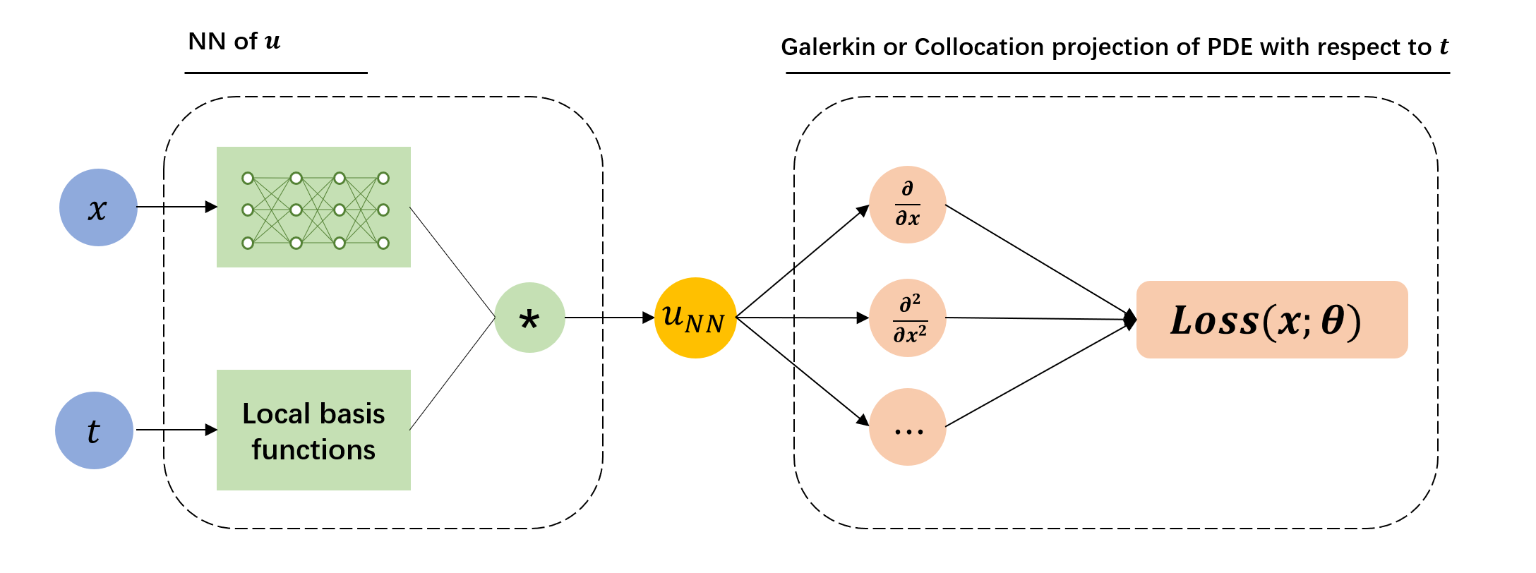
Figure 1: Schematic of the proposed approach.

Algorithm 1 Solving time-dependent PDEs via a hybrid FEM-PINN method

Input: terminal time $T$, number of segment $N_{\mathrm{segment}}$, number of basis function $N$, number of epoch $N_{e}$, training data $S_{r}=\cup_{j=0}^{N}S_{r,j}=\cup_{j=0}^{N}\{\bm{x}_{r,j}^{(i)}\}_{i=1}^{N_{r,j}}$, $S_{ic}=\{\bm{x}_{ic}^{(i)}\}_{i=1}^{N_{ic}}$ and $S_{bc}=\{(\bm{x}_{bc}^{(i)},t_{bc}^{(i)})\}_{i=1}^{N_{bc}}$, initial learning rate $l_{r}$, decay rate $\eta$, step size $n_{s}$

for $k=1,\cdots,N_{\mathrm{segment}}$ do

     Construct $N+1$ local finite element basis functions in the interval $[(k-1)T/N_{\mathrm{segment}},kT/N_{\mathrm{segment}}]$.

     for $j=1,\cdots,N_{e}$ do

         Divide $\{S_{r,j}\}_{j=0}^{N}$, $S_{ic}$ and $S_{bc}$ into $n_{r},n_{ic},n_{bc}$ mini-batches $\{S_{r,j}^{ib}\}_{j=0}^{N},S_{ic}^{ib},S_{bc}^{ib}$ randomly, respectively.

         for $ib=1,\cdots,n$ do

              if $((k-1)N_{e}+j)\%n_{s}==0$ then

                  $l_{r}=\eta*l_{r}$.

              end if

              Compute the loss function ${\widehat{\mathcal{L}}}(\theta)$ (28) for mini-batch data $\{S_{r,j}^{ib}\}_{j=0}^{N},S_{ic}^{ib}$ and $S_{bc}^{ib}$.

              Update $\bm{\theta}$ by using the Adam optimizer.

         end for

     end for

     Compute the prediction for new initial training data set $\{\bm{x}_{ic}^{(i)},t_{ic}^{(i)}\}_{i=1}^{N_{ic}}$, where $t_{ic}^{(i)}=KT/N_{\mathrm{segment}}$.

     Update the above prediction values as $g(\bm{x}_{ic}^{(i)})$.

     Update the corresponding initial and boundary training data $S_{ic},S_{bc}$.

     Save the parameter $\theta$ as $\theta_{k}$.

end for

Output: The predicted solutions $\{u(\bm{x},t_{k};\theta_{k})\}_{k=1}^{N_{\mathrm{segment}}}$, where $t_{k}\in[(k-1)T/N_{\mathrm{segment}},kT/N_{\mathrm{segment}}],k=1,\cdots,N_{\mathrm{segment}}$.

3.1.1 Some remarks on the hybrid form

PINN is formulated as a least-square method in terms of the hypothesis space given by the neural network. The error of $u_{N}(\bm{x},t;\hat{\theta})$ satisfies

$$\mathbb{E}\|u_{\text{exact}}(\bm{x},t)-u_{N}(\bm{x},t;\hat{\theta})\|\leq\|u_{\text{exact}}(\bm{x},t)-u_{N}(\bm{x},t;\theta^{*})\|+\mathbb{E}\|u_{N}(\bm{x},t;\theta^{*})-u_{N}(\bm{x},t;\hat{\theta})\|$$ (31)

for a proper norm, where $\theta^{*}$ is the minimizer of $\mathcal{L}(\theta)$, $\hat{\theta}$ is the minimizer of $\widehat{\mathcal{L}}(\theta)$ and the expectation $\mathbb{E}[\cdot]$ is with respect to random samples. On the right-hand side, the first term is the approximation error determined by the hypothesis space and the second term is the statistical error introduced by the random samples.

It is well known that PINN may fail to predict convection when the frequency is large although the hypothesis space is capable of yielding a good approximate solution [8]. According to the inequality (31), the reason is twofold: the non-convex structure of the loss landscape and the statistical error. First, the best approximation may not be obtained due to non-convexity of the loss function even the statistical error is zero. The change of the loss landscape can be achieved by adding a regularization term. For example, bc-PINNs have a penalty term to force the model to remember what was learned before [9]. Second, the available strategies that improve the performance of PINNs for time integration can be understood through the reduction of statistical error. Assume that $N_{t}$ random samples are used in the time direction. The most straightforward strategy is to divide the time interval as $[0,T]=\cup_{i=0}^{n-1}[i\Delta T,(i+1)\Delta T]$ with $\Delta T=T/n$ and train the model sequentially in each time segment. After such a decomposition, the variation in time is reduced implying that the Monte Carlo approximation of the loss given by the random samples is more accurate due to variance reduction. The better the loss is discretized by random samples, the smaller the statistical error is. Another strategy, called causal training, is proposed in [10]. A weighted residual loss function is defined as

$$\mathcal{L}_{r}(\theta)=\frac{1}{N_{t}}\sum_{i=1}^{N_{t}}\lambda_{i}\mathcal{L}_{r}(t_{i},\theta),$$

where $\mathcal{L}_{r}(t_{i},\theta)$ is the residual loss at $t=t_{i}$, and

$$\lambda_{i}=\exp\left(-\epsilon\sum_{j=1}^{i-1}\mathcal{L}_{r}(t_{j},\theta)\right),\quad i=2,3,\ldots,N_{t}$$

with $0<\epsilon<\infty$. The intuition is that the model will not be trained until the model is well trained for small $t_{i}$, which is consistent with the causality induced by evolution. Note that

$$\frac{1}{N_{t}}\sum_{i=1}^{N_{t}}\lambda_{i}\mathcal{L}_{r}(t_{i},\theta)\approx\frac{1}{T}\int_{t}\lambda(t)\mathcal{L}_{r}(t,\theta)dt$$

is the Monte Carlo approximation of a weighted loss with $N_{t}$ uniform random samples. If $\lambda(t)>0$ and the exact solution is included in the hypothesis space, the same $\theta^{*}$ will be reached. $\lambda(t)$ is a decreasing function by definition while $\mathcal{L}_{r}(t,\theta)$ is in general an increasing function due to the accumulation of errors with time. If $\lambda(t)$ and $\mathcal{L}_{r}(t,\theta)$ are well balanced, their product varies much less in time, corresponding to a small variance in terms of the uniform distribution. Such a balance is mainly achieved by the selection of the so-called causality parameter $\epsilon$. If $\epsilon$ fails to introduce a variance reduction for $\lambda(t)\mathcal{L}_{r}(t,\theta)$, the statistical error will not be reduced, implying that the training results may get worse. This explains the sensitivity of the training strategy on $\epsilon$.

Based on the above observations, we intend to use the hybrid form (15) to alleviate the difficulties induced by the statistical errors in the time direction. We also note that the coefficients for the time finite element basis functions are given by the outputs of a neural network, which corresponds to learning a set of reduced basis functions in the physical space since the output layer of the neural network is a linear combination of these basis functions.

3.2 Deep adaptive sampling method

Random samples are used for the integration in the physical space. To reduce the statistical errors, we consider the adaptive sampling method [29, 30]. For simplicity, we only consider the interior residual $\mathcal{L}_{r}(\theta)$, and the time interval is $[0,1]$. As suggested in [29], we relax the objective function $\mathcal{L}_{r}(\theta)$ as:

$$\widetilde{\mathcal{L}}_{r}(\theta)=\sum_{i=0}^{N}\lambda_{i}\widetilde{\mathcal{L}}_{r,i}(\theta)=\sum_{i=0}^{N}\lambda_{i}\int_{\Omega}r_{i}^{2}(\bm{x};\theta)p_{i}(\bm{x})d\bm{x}\approx\frac{1}{N_{r}}\sum_{i=0}^{N}\sum_{j=1}^{N_{r}}\lambda_{i}r_{i}^{2}(\bm{x}^{(i)}_{j};\theta),$$ (32)

where $\lambda_{i}>0$, $\sum_{i=0}^{N}\lambda_{i}=1$, the set $\{\bm{x}^{(i)}_{j}\}_{j=1}^{N_{r}}$ is generated with respect to the probability density function $p_{i}(\bm{x})>0$ instead of a uniform distribution. We associate $\widetilde{\mathcal{L}}_{r,i}(\theta)$ with a weight $\lambda_{i}$. The minimizer of $\widetilde{\mathcal{L}}_{r}(\theta)$ is also the solution to the problem if the exact solution is included in the hypothesis space. To reduce the error induced by the Monte Carlo approximation, we may adjust $p_{i}(\bm{x})$ to make the residuals $r_{i}^{2}(\bm{x};\theta)$ nearly uniform. To do this, we refine the training set gradually by adding new samples according to the distribution induced by $r_{i}^{2}(\bm{x};\theta^{(k)}$), where $k$ indicates the adaptivity iteration and $\theta^{(k)}$ is the optimal model parameter given by the previous training set. Once the training set is updated, the model will be retrained, based on which the training set will be refined again. In a nutshell, the model and the training set are updated alternately.

The main problem is that we need to obtain new samples from $N+1$ distributions induced by $r_{i}^{2}(\bm{x};\theta^{(k)})$. To handle this issue, we adopt a time-dependent density estimation strategy. Specifically, we augment the spatial variable in different terms ($\widetilde{\mathcal{L}}_{r,i}$) with an extra dimension $s$, and consider a set $\{s_{i}\}_{i=0}^{N}$ of grid points on the time interval. For the Galerkin approach, $s_{i}$ can be interpreted as pre-defined nodes of finite element mesh; for the collocation approach, $s_{i}$ can be viewed as a reordering of pre-defined Gaussian nodes $s_{m,k}$ (see Section 2.2.2). We define a weighted empirical measure

$$\delta_{\lambda}(A)=\sum_{i=0}^{N}\lambda_{i}\delta_{s_{i}}(A)$$

for any $A\subset[0,1]$ with $\delta_{s_{i}}$ being the Dirac measure and let $r(\bm{x},s;\theta)$ be an interpolation function satisfying

$$r(\bm{x},s;\theta)=r_{i}(\bm{x};\theta)\quad\mathrm{if}\;s=s_{i},\quad i=0,\cdots,N.$$ (33)

Let $p_{\bm{X},S}(\bm{x},s)=p_{\bm{X}|S}(\bm{x}|s)p_{S}(s)$ be a joint PDF. Choosing $p_{S}(s)ds=\delta_{\lambda}(ds)$. We have

$$\int\int_{\Omega}r^{2}(\bm{x},s;\theta)p_{\bm{X},S}(\bm{x},s)\mathrm{d}\bm{x}\mathrm{d}s=\sum_{i=0}^{N}\int_{\Omega}r_{i}^{2}(\bm{x};\theta)p_{\bm{X}|S}(\bm{x}|s_{i})\lambda_{i}\mathrm{d}\bm{x},$$ (34)

which is consistent with equation (32) if $p_{\bm{X}|S}(\bm{x}|s_{i})=p_{i}(\bm{x})$. Using $p_{\bm{X},S}(\bm{x},s)$, the objective functional is discretized as

$$\widetilde{\mathcal{L}}_{r}(\theta)\approx\frac{1}{N_{r}}\sum_{i=1}^{N_{r}}r^{2}(\bm{x}^{(i)},s^{(i)};\theta),$$ (35)

where $\{(\bm{x}^{(i)},s^{(i)})\}_{i=1}^{N_{r}}$ are sampled from $p_{\bm{X},S}(\bm{x},s)$. We will use a density model with the form $p_{\bm{X}|S}(\bm{x}|s)p_{S}(s)$ to approximate the distribution induced by $r^{2}(\bm{x},s;\theta)$. New samples from the trained density model will be added to the training set for refinement.

3.2.1 Model $p_{S}(s)$

Without loss of generality, we assume that $s\in[0,1]$. We aim to find a invertible transformation $z=f(s)$ such that

$$\quad p_{S}(s)=p_{Z}(f(s))|\det\nabla_{s}f|,\quad Z\sim\mathcal{U}[0,1],$$ (36)

where $\mathcal{U}$ denotes the uniform distribution. We use the bounded polynomial spline layer $f_{\mathrm{poly}}$ [31] to parameterize $f$. Specifically, let $0=l_{0}<l_{1}<\cdots<l_{m-1}<l_{m}=1$ be a given partition of the unit interval and $\{k_{j}\}_{j=0}^{m}$ be the corresponding weights satisfying $\sum_{j}k_{j}=1$. A piecewise linear polynomial can be defined as follows:

$$p(s)=\frac{k_{j+1}-k_{j}}{l_{j+1}-l_{j}}(s-l_{j})+k_{j},\quad\forall s\in[l_{j},l_{j+1}].$$ (37)

Then the corresponding cumulative probability function $f_{\mathrm{poly}}$ admits the following formulation:

$$f_{\mathrm{poly}}(s)=\frac{k_{j+1}-k_{j}}{2(l_{j+1}-l_{j})}(s-l_{j})^{2}+k_{j}(s-l_{j})+\sum_{i=0}^{j-1}\frac{k_{i}+k_{i+1}}{2}(l_{i+1}-l_{i}),\quad\forall s\in[l_{j},l_{j+1}].$$ (38)

To satisfy $\int_{0}^{1}p(s){\rm d}s=1$, we can model $\{k_{j}\}_{j=0}^{m}$ as

$$k_{j}=\frac{\exp(\tilde{k}_{j})}{C},\ \forall j=0,\ldots,m,$$ (39)

where $\theta_{f,1}=\{\tilde{k}_{j}\}_{j=0}^{m}$ are trainable parameters and $C$ is a normalization constant:

$$C=\sum_{i=0}^{m-1}\frac{(\exp(\tilde{k}_{i})+\exp(\tilde{k}_{i+1}))(l_{i+1}-l_{i})}{2}.$$ (40)

Notice that the polynomial spline layer $f_{\mathrm{poly}}(\cdot;\theta_{f,1})$ (37)-(38) yields explicit monotonous expressions, and its inverse can be readily computed. Then an explicit PDF model $p_{\mathrm{poly}}(s;\theta_{f,1})$ can be obtained by letting $f=f_{\mathrm{poly}}$, i.e.,

$$p_{\mathrm{poly}}(s;\theta_{f,1})=p_{Z}(f_{\mathrm{poly}}(s))\left|\det\nabla_{s}f_{\mathrm{poly}}\right|.$$ (41)

3.2.2 Model $p_{X|S}(\textbf{x}|s)$

For $\bm{x}\in\mathbb{R}^{d}$, we seek a invertible transformation $\bm{z}=f(\bm{x},s)\in\mathbb{R}^{d}$ for any given $s$ such that

$$p_{\bm{X}|S}(\bm{x}|s)=p_{\bm{Z}|S}(\bm{z}|s)\left|\frac{\partial f(\bm{x},s)}{\partial\bm{x}}\right|,\quad\bm{Z}|S\sim\mathcal{U}[-1,1]^{d},\quad\forall s.$$ (42)

Here we employ conditional bounded KR-net $f_{\mathrm{B-KRnet}}(\cdot,s)$ [32] to parameterize $f(\cdot,s)$. The basic idea of conditional bounded KRnet is to define the structure of $f(\bm{x},s)$ in terms of the Knothe-Rosenblatt rearrangement. The transformation $f(\cdot,s)$ inspired by the Knothe-Rosenblatt (K-R) rearrangement [33] has a low-triangular structure

$$\bm{z}=f(\bm{x},s)=\left[\begin{array}[]{l}f_{1}(x_{1},s)\\ f_{2}(x_{1},x_{2},s)\\ \vdots\\ f_{d}(x_{1},\cdots,x_{d},s)\end{array}\right].$$ (43)

The sub-transformations $f_{1},\cdots,f_{d}$ consist of polynomial spline layers and coupling layers [34]. More details can be found in [32, 35]. Let $f_{\mathrm{B-KRnet}}(\cdot,s;\theta_{f,2})$ indicate the conditional invertible transport map induced by bounded KR-net, where $\theta_{f,2}$ includes the model parameters. Then an explicit PDF model $p_{\mathrm{B-KRnet}}(\bm{x},s;\theta_{f,2})$ can be obtained by letting $f=f_{\mathrm{B-KRnet}}$ in equation (42)

$$p_{\mathrm{B-KRnet}}(\bm{x}|s;\theta_{f,2})=p_{\bm{Z}}(f_{\mathrm{B-KRnet}}(\bm{x},s))\left|\det\nabla_{\bm{x}}f_{\mathrm{B-KRnet}}\right|.$$ (44)

3.2.3 Adaptive sampling approach

Now we model a continuous joint density distribution $p_{\theta_{f}}(\bm{x},t)$

$$p_{\theta_{f}}(\bm{x},t)=p_{\mathrm{poly}}(t;\theta_{f,1})p_{\mathrm{B-KRnet}}(\bm{x}|t;\theta_{f,2}),$$ (45)

where $\theta_{f}=\{\theta_{f,1},\theta_{f,2}\}$. To seek the "optimal" parameter $\theta_{f}$, we can minimize the following objective

$$D_{\mathrm{KL}}(\hat{r}_{\theta}(\bm{x},t)||p_{\theta_{f}}(\bm{x},t)) =D_{\mathrm{KL}}\big{(}\hat{r}_{\theta}(\bm{x},t)||p_{\mathrm{poly}}(t;\theta_{f,1})p_{\mathrm{B-KRnet}}(\bm{x}|t;\theta_{f,2})\big{)}$$ (46)

$$=\iint\hat{r}_{\theta}(\bm{x},t)\log\left(\hat{r}_{\theta}(\bm{x},t)\right)\mathrm{d}\bm{x}\mathrm{d}t-\iint\hat{r}_{\theta}(\bm{x},t)\log\left(p_{\mathrm{poly}}(t;\theta_{f,1})p_{\mathrm{B-KRnet}}(\bm{x}|t;\theta_{f,2})\right)\mathrm{d}\bm{x}\mathrm{d}t,$$

where $D_{\mathrm{KL}}$ indicates the Kullback-Leibler (KL) divergence and $\hat{r}_{\theta}(\bm{x},t)\propto r^{2}(\bm{x},t;\theta)$ is the induced measure by continuous residual squared $r^{2}(\bm{x},t;\theta)$

$$r(\bm{x},t;\theta)=\partial_{t}u_{N}(\bm{x},t;\theta)-\mathcal{N}[u_{N}](\bm{x},t;\theta)-f(\bm{x},t).$$

The first term on the right-hand side in (46) corresponds to the differential entropy of $\hat{r}_{\theta}(\bm{x},t)$, which does not affect the optimization with respect to $\theta_{f}$. So minimizing the KL divergence is equivalent to minimizing the cross entropy between $\hat{r}_{\theta}(\bm{x},t)$ and $p_{\theta_{f}}(\bm{x},t)$

$$H(\hat{r}_{\theta}(\bm{x},t),p_{\theta_{f}}(\bm{x},t)) =-\iint\hat{r}_{\theta}(\bm{x},t)\log\left(p_{\mathrm{poly}}(t;\theta_{f,1})p_{\mathrm{B-KRnet}}(\bm{x}|t;\theta_{f,2})\right)\mathrm{d}\bm{x}\mathrm{d}t,$$ (47)

Since the samples from $\hat{r}_{\theta}(\bm{x},t)$ are not available, we approximate the cross entropy using the importance sampling technique:

$$H(\hat{r}_{\theta}(\bm{x},t),p_{\theta_{f}}(\bm{x},t))\approx-\frac{1}{N_{r}}\sum_{i=1}^{N_{r}}\frac{\hat{r}_{\theta}(\bm{x}_{i},t_{i})}{p_{\mathrm{poly}}(t_{i};\hat{\theta}_{f,1})p_{\mathrm{B-KRnet}}(\bm{x}_{i}|t_{i};\hat{\theta}_{f,2})}\left(\log p_{\mathrm{poly}}(t_{i};\theta_{f,1})+\log p_{\mathrm{B-KRnet}}(\bm{x}_{i}|t_{i};{\theta}_{f,2})\right),$$ (48)

where

$$t_{i}\sim p_{\mathrm{poly}}(\cdot;\hat{\theta}_{f,1}),\quad\bm{x}_{i}\sim p_{\mathrm{B-KRnet}}(\cdot|t_{i};\hat{\theta}_{f,2}).$$ (49)

The choice of $\hat{\theta}_{f}=\{\hat{\theta}_{f,1},\hat{\theta}_{f,2}\}$ will be specified as follows.

Once obtaining the well-trained parameters $\theta_{f}^{*}=\{\theta_{f,1}^{*},\theta_{f,2}^{*}\}$, one can refine initial training set via adding new samples and update the weights in (32). Specifically, note that the residuals $r_{i}(\bm{x};\theta)$ in (27) are only needed at time $s_{i}$, we need to construct the corresponding discrete distributions. For system (19) in Galerkin projection, we use the following discrete distribution

$$p_{\mathrm{dis}}(s)=\left\{\begin{array}[]{rl}\frac{\int_{\Omega}r_{i}^{2}(\bm{x};\theta)\mathrm{d}\bm{x}}{\sum_{i=0}^{N}\int_{\Omega}r_{i}^{2}(\bm{x};\theta)\mathrm{d}\bm{x}},&s=s_{i},0\leq i\leq N\\ 0,&\mathrm{otherwise}.\end{array}\right.$$ (50)

For system (22) in collocation projection, we simply use the following discrete distribution

$$p_{\mathrm{dis}}(s;\theta_{f,1}^{*})=\left\{\begin{array}[]{rl}\int_{0}^{(s_{0}+s_{1})/2}p_{\mathrm{poly}}(s;\theta_{f,1}^{*})\mathrm{d}s,&s=s_{0},\\ \int_{(s_{i-1}+s_{i})/2}^{(s_{i}+s_{i+1})/2}p_{\mathrm{poly}}(s;\theta_{f,1}^{*})\mathrm{d}s,&s=s_{i},0<i<N\\ \int_{(s_{N-1}+s_{N})/2}^{1}p_{\mathrm{poly}}(s;\theta_{f,1}^{*})\mathrm{d}s,&s=s_{N},\\ 0,&\mathrm{otherwise}.\end{array}\right.$$ (51)

Then the weights in (32) can be determined via the discrete distribution $p_{\mathrm{dis}}(\cdot;\theta_{f,1}^{*})$. For collocation projection, it is straightforward to refine the training set. We first generate $N_{\mathrm{new}}$ samples $\{t_{j}\}_{j=1}^{N_{\mathrm{new}}}$ via the well-trained model $p_{\mathrm{dis}}(\cdot;\theta^{*}_{f,1})$, then we generate the corresponding spatial samples $\bm{x}_{j}\sim p_{\mathrm{B-KRnet}}(\cdot|t_{j};\theta^{*}_{f,2})$ for each $t_{j}$. After that we reorder newly generated data into the original spatial space

$$\bm{x}_{j}\in S^{(i)}_{r,\mathrm{new}},\quad\mathrm{if}\;t_{j}=s_{i},\forall i=0,\cdots,N,\;j=1,\cdots,N_{\mathrm{new}}.$$ (52)

For Galerkin projection, recall that we need to use the same training set for the basis function with same support (see (25)). Hence for each $s_{i}$ in (50), one firstly identies its corresponding basis function and support, here it is denoted as $\tilde{I}_{i}$. Then we generate spatial samples $\bm{x}_{i,k}\sim p_{\mathrm{B-KRnet}}(\cdot|t_{i,k};\theta_{f,2}^{*})$, where $t_{i,k}$ are Gaussian quadrature points in the interval $\tilde{I}_{i}$. The total number of generated spatial points for each $s_{i}$ should be proportional to the discrete weights $p_{\mathrm{dis}}(s_{i})$. Again, we recoder newly generated data into the original spatial space

$$\bm{x}_{i,k}\in S^{(i)}_{r,\mathrm{new}},\quad\forall i=0,\cdots,N.$$ (53)

We are now ready to present our algorithms. Let $\{S_{r,0}^{(i)}\}_{i=0}^{N},S_{ic}$ and $S_{bc}$ be three sets of collocation points that are uniformly sampled from $\Omega^{N+1}$, $\Omega\times\{0\}$ and $\partial\Omega\times[0,T]$, respectively. Using $\{S_{r,0}^{(i)}\}_{i=0}^{N},S_{ic}$ and $S_{bc}$, we minimize the empirical loss (28) to obtain $u(\bm{x},t;\theta^{*,(1)})$. With $u(\bm{x},t;\theta^{*,(1)})$, we minimize the cross entropy (48) to get $p_{\theta^{*,(1)}_{f}}(\bm{x},t)$, where we use uniform samples for importance sampling. To refine the training set, a new set $S_{r,\mathrm{new}}=\{S^{(i)}_{r,\mathrm{new}}\}_{i=0}^{N}$ is generated according to the model $p_{\theta_{f}^{*,(1)}}(\bm{x},t)$, and new training set can be updated as $S_{r,1}=S_{r,0}\cup S_{r,\mathrm{new}}$. Then we continue to update the approximate solution $u(\bm{x},t;\theta^{*,(1)})$ using $S_{r,1}$ as the training set, which yields a refined model $u(\bm{x},t;\theta^{*,(2)})$. Starting from $k=2$, we seek $p_{\theta^{*,k}}(\bm{x},t)$ using the previous approach. We repeat the procedure to obtain an adaptive algorithm (see Algorithm 2).

Algorithm 2 Deep adaptive sampling method for time-dependent PDEs

Input: Initial $p_{\mathrm{dis}}(t;\theta_{f,1}^{(0)}),p_{\mathrm{B-KRnet}}(\bm{x},t;\theta_{f,2}^{(0)})$,$u(\bm{x},t;\theta)$, number of finite element basis $N+1$, initial weights $\lambda_{i}=\frac{1}{N+1}$, maximum epoch number $N_{e}$, number of maximum iteration $N_{\mathrm{adaptive}}$, number of newly added points $N_{\mathrm{new}}$, training data $\{S_{r,0}^{(i)}\}_{i=0}^{N}$, $S_{ic}$ and $S_{bc}$.

for $k=0,\cdots,N_{\mathrm{adaptive}}-1$ do

     // Solve PDE

     for $j=1,\cdots,N_{e}$ do

         Divide $\{S_{r,k}^{(i)}\}_{i=0}^{N}$, $S_{ic}$ and $S_{bc}$ into $n_{r},n_{ic},n_{bc}$ mini-batches $\{S_{r,k}^{(i),ib}\}_{i=0}^{N},S_{ic}^{ib},S_{bc}^{ib}$ randomly, respectively.

         for $ib=1,\cdots,n$ do

              Compute the loss function ${\widehat{\mathcal{L}}}(\theta)$ (35) for mini-batch data $\{S_{r,k}^{(i),ib}\}_{i=0}^{N},S_{ic}^{ib}$ and $S_{bc}^{ib}$.

              Update $\theta$ by using the Adam optimizer.

         end for

     end for

     // Train density model

     for $j=1,\cdots,N_{e}$ do

         Sample $n_{r}$ samples from $\{S_{r,k}^{(i),ib}\}_{i=0}^{N}$

         Update $p_{\mathrm{poly}}(t;\theta_{f,1}^{(k)})$ and $p_{\mathrm{B-KRnet}}(\bm{x}|t;\theta_{f,2}^{(k)})$ by descending the stochastic gradient of $H(\hat{r}_{\theta}(\bm{x},t),p_{\theta_{f}^{(k)}}(\bm{x},t))$ (see equation (48))

     end for

     // Refine training set and update weights

     Generate $N_{\mathrm{new}}\times(N+1)$ samples $\{S_{r,\mathrm{new}}^{(i)}\}_{i=0}^{N}$, where $t_{j}\sim p_{\mathrm{dis}}(\cdot;\theta_{f,1}^{(k)})$ and $\bm{x}_{j}\sim p_{\mathrm{B-KRnet}}(\cdot|t_{j};\theta^{(k)}_{f,2})$.

     $\{S_{r,k+1}^{(i)}\}_{i=0}^{N}=\{S_{r,k}^{(i)}\}_{i=0}^{N}\cup\{S_{r,\mathrm{new}}^{(i)}\}_{i=0}^{N}$.

end for

Output: The predicted solution $u(\bm{x},t;\theta^{*})$.

4 Numerical experiments

In this section, we conduct some numerical experiments to demonstrate the effectiveness of the proposed method, including one convection equation, one Allen-Cahn equation, one two-dimensional and low regularity test problems, and two high-dimensional linear or nonlinear problems. Throughout all benchmarks, we will employ the fully-connected neural network equipped with hyperbolic tangent activation functions (Tanh) and initialized using the Glorot normal scheme [36]. All neural networks are trained via stochastic gradient descent using the Adam optimizer with default settings [37] and an exponential learning rate decay with a decay-rate of 0.9 every 1,000 training iterations. All experiments are implemented by JAX [38].

In order to test the validity of the method, we use the following relative $L_{2}$ error:

$$err_{L_{2}}=\frac{\sqrt{\sum_{i=1}^{\mathrm{num}}|u(\bm{x}_{i},t_{i};\theta)-u(\bm{x}_{i},t_{i})|^{2}}}{\sqrt{\sum_{i=1}^{\mathrm{num}}|u(\bm{x}_{i},t_{i})|^{2}}},$$ (54)

where $\mathrm{num}$ represents the total number of test points chosen randomly in the domain, and $u(\bm{x}_{i},t_{i};\theta)$ and $u(\bm{x}_{i},t_{i})$ represent the predicted and the exact solution values, respectively.

4.1 Convection equation

We start with a one-dimensional linear convection equation of the form

$$\frac{\partial u}{\partial t}+\beta\frac{\partial u}{\partial x}=0,\quad(x,t)\in[0,2\pi]\times[0,1],$$ (55)

subject to periodic boundary conditions and an initial condition $u(0,x)=\sin(x)$. The precise solutions for varying values of $\beta$ are depicted in Figure 2. One can observe that as $\beta$ increases, the solution exhibits increasingly pronounced temporal variations.

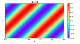
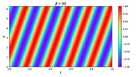
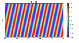
Figure 2: Exact solutions. From left to right: $\beta=10,30$ and $50$.

We initially evaluate the performance with linear finite element basis functions in Galerkin projection. The latent coefficients, denoted as ${\omega_{i}(\bm{x};\theta)}$, are represented using a fully-connected neural network with tanh activation function, 4 hidden layers and 128 neurons per hidden layer. To simplify the training object, we strictly impose the periodic boundary conditions by embedding the input coordinates into Fourier expansion (see A). Notice that the above equation is linear, we use the linear form of loss function (20) and set $N_{\mathrm{segment}}=1$. We create a uniform mesh of size 400 in the spatial computational domain $[0,2\pi]$, yielding 400 initial points and 400 collocation points for enforcing the PDE residual. We proceed by training the resulting model via full-batch gradient descent using the Adam optimizer for 40,000 iterations. As shown in Figure 3, for fixed $N$, the relative $L_{2}$ gradually increases as $\beta$ increases; for fixed $\beta=50$, the relative $L_{2}$ exhibits linear convergence concerning the number of basis functions ($N$). Particularly, when $\beta=30$, the proposed method attains a remarkable relative $L_{2}$ error of $2.85e-3$.

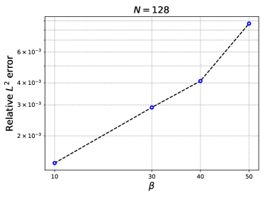
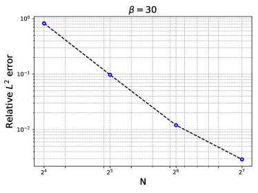
Figure 3: Convection equation. Numerical results with linear finite element discretization.

Furthermore, we investigate the impact of linear and quadratic finite element basis functions on the performance of the proposed model. Specifically, we set $\beta$ to 50 and vary the number of mesh elements $N$, ranging from 32 to 128. We then train the proposed model under same hyperparameter configurations. Figure 4 and Table 1 present a summary of the relative $L_{2}$ errors observed in the trained models. It is not surprising that the error diminishes when we replace linear basis functions with quadratic ones, in accordance with the classical results of finite element theory.

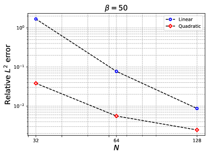
Figure 4: Convection equation ($\beta=50$). Linear finite element basis functions versus quadratic finite element basis functions.

To investigate the effects of increasing the number of basis functions, we compare the relative $L_{2}$ errors given by various settings. It is seen in Table 1 that relative $L_{2}$ error decreases as $N$ increases for all cases.

$N$	32	64	96	128
Galerkin (linear)	1.69e+00	7.73e-02	1.91e-02	8.69e-03
Galerkin (quadratic)	3.83e-02	5.58e-03	2.26e-03	1.13e-03
Collocation (Hermite polynomial)	1.97e-01	1.18e-02	2.34e-03	7.50e-04
Collocation (spline)	6.44e-01	1.83e-02	3.16e-03	9.83e-04

Table 1: Convection equation ($\beta=50$). Relative $L_{2}$ errors at different $N$ for different methods.

In Table 2 we compare the performance of the proposed method with the DABG [24] at different $\beta$. One can observe that for these two methods, when $\beta$ is relatively small, as $N$ increases, the error first decreases and then increases; when $\beta$ is relatively large, the error consistently decreases as $N$ increases. We conjecture that reason for this phenomenon is that when $\beta$ is relatively small (i.e., the solution is smoother), small $N$ can achieve good accuracy, while larger $N$ may lead to greater optimization challenges. Another message from Table 2 is that the proposed approach exhibits reduced sensitivity to temporal frequency variations in the solution compared to DABG.

$N$		8	16	32	64	96	128
$\beta=10$	Galerkin(quadratic)	1.55e-02	3.52e-03	1.03e-03	4.67e-04	6.91e-04	3.91e-01
	DABG	1.36e-02	1.25e-04	8.73e-04	1.04e-05	3.33e+00	1.32e+00
$\beta=30$	Galerkin(quadratic)	3.37e-01	4.98e-02	8.03e-03	1.90e-03	9.03e-04	5.04e-04
	DABG	1.12e+00	2.87e-01	2.93e-04	4.34e-04	5.75e-05	1.06e-04
$\beta=50$	Galerkin(quadratic)	4.67e+00	2.15e-01	3.83e-02	5.17e-03	2.08e-03	1.32e-03
	DABG	1.05e+00	1.03e+00	3.30e-03	1.44e-03	6.46e-04	6.39e-04

Table 2: Convection equation. Different relative $L_{2}$ errors between the proposed method and DABG.

We also compare the performance and computational time of the proposed method with causal PINNs. We set the same hyper parameters to compare these two methods, including the architecture of neural network, the initial learning rate, decay rate, the number of training points in space, and iterations. The $\epsilon$ in causal PINNs is set to $\{1e-2,1e-1,1e0,1e1,1e2\}$. All runtime statistics were computed on the same hardware, a Nvidia Tesla V100 w/ 32 GB memory. It is shown in Table 3 that as $\beta$ increases, the proposed method demonstrates superior accuracy compared to causal PINNs. The proposed method (Galerkin projection) runs approximately 100 times faster than causal PINNs. Such a significant difference in efficiency is due to the distinct computational graphs adopted by these two methods. For the proposed method, because the residual originates from the linear system defined in (20), we can pre-calculate the finite element sparse matrix along the time direction. We consider the computational cost of automatic differentiation in calculating the residual. For any given spatial point $\bm{x}$, causal PINNs need $n$ back-propagation computations for $n$ temporal points, while our method only requires a single back-propagation computation and one matrix-vector multiplication of the above-mentioned finite element sparse matrix and the neural network output.

$\beta$		10	30	50
Error	Galerkin(quadratic)	2.95e-04	1.32e-03	3.57e-03
	Causal PINNs	7.58e-04	1.12e-02	1.65e+00
Running time	Galerkin(quadratic)	57	62	63
	Causal PINNs	6639	8087	8057

Table 3: Convection equation. Relative $L_{2}$ error and running time between the proposed method and causal PINNs.

4.2 Allen-Cahn equation

The next example aims to illustrate the effectiveness of time marching technology in our proposed method. Consider the following Allen-Cahn equation

$$\begin{array}[]{rcl}u_{t}-c_{1}^{2}\nabla^{2}u+f(u)&=&0,\quad x\in[-1,1],t\in[0,1],\\ f(u)&=&c_{2}(u^{3}-u),\\ u(x,0)&=&x^{2}\cos(\pi x),\\ u(1,t)&=&u(-1,t),\\ u_{x}(1,t)&=&u_{x}(-1,t),\end{array}$$ (56)

where $c_{1}^{2}=0.0001$ and $c_{2}=5$. We take the number of linear mesh elements as 100 and represent the latent coefficients $\{\omega_{i}(\bm{x};\theta)\}$ by a fully-connected neural network with tanh activation function, 4 hidden layers and 128 neurons per hidden layer. Similarly, we strictly impose the periodic boundary conditions by embedding the input coordinates into Fourier expansion (see A). We create a uniform mesh of size 1,000 in the spatial computational domain $[-1,1]$, yielding 1,000 initial points and 1,000 collocation points for enforcing the PDE residual. We proceed by training the resulting model via full-batch gradient descent using the Adam optimizer for the total 100,000 iterations. The resulting $L_{2}$ errors for different numbers of time segments are shown in Table 4. We observe the relative $L_{2}$ error significantly decreases as the number of time segments increases. One can see that the predicted solution achieves an excellent agreement with the ground truth, yielding an approximation error of $7.67e-3$ measured in the relative $L_{2}$ norm.

$N_{\mathrm{segment}}$	1	2	4
Error	–	1.17e-02	7.67e-03

Table 4: The relative $L_{2}$ error for different segments. (Linear finite element basis function with $N=100$)

In addition, we employ quadratic basis functions and set $N$ to 30. All other parameters remain consistent with the previous configuration. In Table 5 similar results are observed compared to the previous scenario. Moreover, we also present a representative predicted solution in Figure 5, one can see that the predicted solution is in good agreement with the reference solution.

$N_{\mathrm{segment}}$	1	2	4
Error	2.25e-01	7.57e-03	5.08e-03

Table 5: Relative $L_{2}$ error for different segments. (Quadratic finite element basis function with $N=30$)

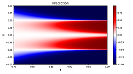
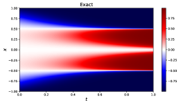
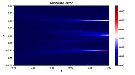
Figure 5: Allen Cahn equation. From left to right: the prediction and absolute error. Relative $L_{2}$ error is 5.08e-3 (Quadratic basis function, $N_{\mathrm{segment}}$=4, $N$=30).

$N$	10	20	30
Galerkin (quadratic)	4.07e-03	7.87e-03	7.57e-03
Collocation (Hermite polynomial)	4.12e-03	5.51e-03	7.65e-03
Collocation (spline)	3.81e-03	3.89e-03	3.56e-03

Table 6: Relative $L_{2}$ error for different approaches ($N_{\mathrm{segment}}=2$).

We summarize some relative $L_{2}$ errors for $N_{\mathrm{segment}}=2$ in Table 6. We observe that the collocation framework with piecewise spline functions has achieved the best accuracy. Moreover, we compare the Galerkin projection with causal PINNs in Table 7. Again, we set the same hyper parameters to compare these two methods. The $\epsilon$ in causal PINNs is set to $\{1e-2,1e-1,1e0,1e1,1e2\}$. It is shown that the accuracy of these two methods is comparable. Note that due to the presence of non-linear term $f(u)$, we must employ a Gaussian quadrature formula of a sufficient degree of exactness for the Galerkin projection in the time direction. Even so, the proposed method runs approximately 40 times faster than causal PINNs.

	Galerkin(quadratic)	Causal PINNs
Running time	71	2524
Error ($N_{\mathrm{segment}}$=1)	1.95e-02	1.33e-02
Error ($N_{\mathrm{segment}}$=2)	3.58e-03	3.73e-03

Table 7: Relative $L_{2}$ error and running time for the proposed method and causal PINNs.

4.3 High-dimensional linear problem

To demonstrate the effectiveness of the proposed approaches in tackling high-dimensional PDEs, we consider the following parabolic equation with non-constant coefficients

$$u_{t}-\nabla\cdot(a(\bm{x})\nabla u)=f,\quad\mbox{in }\Omega\times(0,1],$$ (57)

$$u(\bm{x},0)=0,\quad\mbox{in }\Omega,$$

$$u=0,\quad\mbox{on }\partial\Omega\times[0,1],$$

with $a(\bm{x})=1+|\bm{x}|^{2}/2$. The domain is set to be the 20-D unit ball $\Omega=\{\bm{x}\in\mathbb{R}^{20}\mid|\bm{x}|<1\}$, and the true solution is set to be

$$u(\bm{x},t)=\sin\big(\sin(2\pi\omega t)(|\bm{x}|^{2}-1)\big{missing}).$$ (58)

We set $\omega$ to be 3 and $N_{\mathrm{segment}}$ to be 1. For simplicity, here we only test the performance of the proposed approach with quadratic finite element basis functions. We represent the latent coefficients $\{{\omega}_{i}(\bm{x};\theta)\}$ by a fully-connected neural network with activation function tanh, 5 hidden layers, and 128 neurons per hidden layer. We impose exactly the Dirichlet boundary conditions by transforming the output into the following form:

$${\omega}_{i}(\bm{x};\theta)={\omega}_{i}(\bm{x};\theta)(|\bm{x}|-1).$$ (59)

In addition, we set $\tilde{u}_{0}(\bm{x};\theta)$ to be zero such that the initial conditions are exactly satisfied. To obtain a set of training data for evaluating PDE residual, we randomly sample 100,000 collocation points in $\Omega$. Since the problem is linear, equation (20) is used to define the loss. We set the size of mini-batch to 5,000 and train the model via mini-batch stochastic descent with the Adam optimizer for 40,000 iterations. The corresponding results for different numbers of mesh elements are summarized in Table 8. We observe that the resulting relative $L_{2}$ error is $9.67e-4$, which is more accurate than the ones in recent work [24] ($3.07e-3$ for the deep adaptive basis Galerkin approach and $4.54e-2$ for the PINNs).

N	10	20	40	80
Galerkin (quadratic)	4.45e-02	7.61e-03	1.74e-03	9.67e-04
Collocation (Hermite polynomial)	2.28e-02	1.41e-03	6.58e-04	1.04e-03
Collocation (spline)	4.89e-02	1.42e-02	6.42e-04	8.89e-04

Table 8: Relative $L_{2}$ error for different $N$.

4.4 High-dimensional nonlinear problem

In this case, we solve the Allen-Cahn equation

$$u_{t}-\Delta u+u^{3}-u=f_{AC},\quad\mbox{in }\Omega\times[0,1],$$ (60)

$$u(\bm{x},0)=0,\quad\mbox{in }\Omega,$$

$$u=0,\quad\mbox{on }\partial\Omega\times[0,1].$$

The domain is set as $\Omega=\{\bm{x}\in\mathbb{R}^{20}:|\bm{x}|<1\}$, and the true solution is set to be

$$u(\bm{x},t)=\sin(\sin(2\pi\omega t)(|\bm{x}|^{2}-1)).$$

Here we set $\omega$ to be 3 and $N_{\mathrm{segment}}$ to be 1. For simplicity, We only test the performance of the proposed approach with quadratic finite element basis functions. We represent the latent coefficients $\{\tilde{u}_{i}(\bm{x};\theta)\}$ by a fully-connected neural network with tanh activation function, 5 hidden layers and 128 neurons per hidden layer. The initial condition and Dirichlet boundary condition can be exactly embedded into the network structure (as described in Section 4.3). We set $K$ in equation (13) to be 30 and randomly sample 100,000 collocation points for evaluating PDE residual. We set mini-batch to be 5,000 and proceed by training the resulting model via stochastic gradient descent using the Adam optimizer for 40,000 iterations. The obtained errors for different number of finite element $N$ are shown in Table 9. The resulting relative $L_{2}$ error is $1.16e-3$, which is more accurate than the recent ones in [24] ($2.07e-3$ for the deep adaptive basis Galerkin approach and $7.79e-2$ for the PINNs).

N	10	20	40	80
Galerkin (quadratic)	4.48e-02	7.92e-03	1.89e-03	1.16e-03
Collocation (Hermite polynomial)	2.48e-02	2.21e-03	1.72e-03	1.33e-03
Collocation (spline)	5.04e-02	1.61e-02	2.42e-03	2.31e-03

Table 9: Relative $L_{2}$ error for different $N$.

4.5 Low regularity test problems

Our last example aims to demonstrate the effectiveness of the proposed adaptivity strategy. We consider the following low-regularity equation

$$u_{t}-\Delta u=f\quad\mbox{in }\Omega\times(0,T]$$

$$u(x_{1},x_{2};0)=g(x_{1},x_{2})\quad\mbox{in }\Omega\times\{0\},$$

$$u(x_{1},x_{2};t)=h(x_{1},x_{2};t)\quad\mbox{on }\partial\Omega\times(0,T].$$

where $\Omega=[0,1]^{2},T=0.5$ and the true solution is chosen as

$$u(x_{1},x_{2},t)=\exp\big(-\beta\left[(x_{1}-t-1/4)^{2}+(x_{2}-t-1/4)^{2}\right]\big{missing}).$$

This solution has one peak at the point $(t+1/4,t+1/4)$ and decreases rapidly away from $(t+1/4,t+1/4)$, see Figure 6.

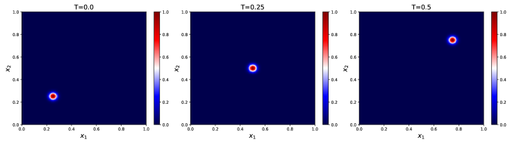
Figure 6: Exact solutions for different time ($\beta$=1000). From left to right: $t=0,0.25$ and $0.5$.

We first consider the case with $\beta=200$. We represent the latent coefficients $\{\tilde{\omega}_{i}(\bm{x};\theta)\}$ by a fully-connected neural network with activation function tanh, 5 hidden layers and 128 neurons per hidden layer. To simplify the training objective, we precisely embed the Dirichlet boundary conditions into the neural network architecture through the following transformation

$$\tilde{\omega}_{i}(\bm{x};\theta)=x_{1}x_{2}(1-x_{1})(1-x_{2})\tilde{\omega}_{i}(\bm{x};\theta).$$

For B-KRnet, we take 8 CDF coupling layers, and two fully connected layers with 32 neurons for each CDF coupling layer. The corresponding activation function is tanh. To assess the effectiveness of our adaptive sampling approach, we generate a uniform meshgrid with size $256\times 256\times 100$ in $[0,1]^{2}\times[0,0.5]$ and compute relative $L_{2}$ error on these grid points.

For collocation projection, we set the number of piecewise cubic spline basis functions to 20, and randomly sample 1,000 collocation points in $\Omega$ as our initial training set. We let $N_{\mathrm{adaptive}}=5$ and $N_{\mathrm{new}}=500$. The number of epochs for training $u(\bm{x},t;\theta)$ and $p_{\theta_{f}}(\bm{x},t)$ is set to 40,000 and 5,000, respectively.

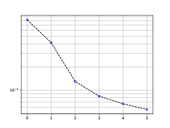
Figure 7: Relative $L_{2}$ error of different adaptivity iterations for collocation projection.

In Figure 7, we plot the approximation errors with respect to the adaptivity iterations. It is clearly seen that the error rapidly decreases as the adaptivity iteration step $k$ increases. Figure 8 shows the evolution of temporal distribution $p_{\mathrm{dis}}(t)$ for $k=1,3,5$. It is seen that the largest density at the first adaptivity iteration is around terminal time. After the training set is refined, the error profile becomes more flat at $k=3$ and $5$. Similar results are observed in Figure 9, which indicates that the distribution of residual becomes more uniform as adaptivity iteration increases.

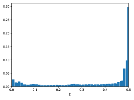
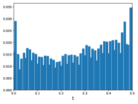
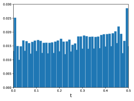
Figure 8: Temporal density of the 1st, 3rd, 5th adaptivity iteration. ($\beta=200$, collocation projection)

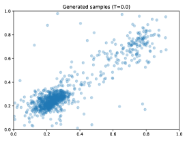
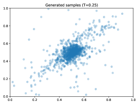
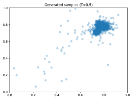
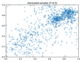
Figure 9: From top to bottom: The generated samples of the 1st and 5th adaptivity iteration. ($\beta=200$, collocation projection)

For Galerkin projection, we set the number of piecewise quadratic basis functions to 20, the remaining hyper-parameter settings remain the same. The corresponding numerical results, included in B, are very similar to the results for collocation projection.

We also investigate the case when $\beta=1000$. Here we take the Galerkin projection as an example.

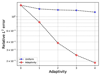
Figure 10: Relative $L_{2}$ error for different sampling strategies ($\beta$=1000, Galerkin projection).

In Figure 10, we compare the performance of uniform sampling and adaptive sampling using the relative $L_{2}$ error, which demonstrates the necessity of adaptive sampling for this case. Figure 11 shows the evolution of temporal weights $\lambda_{i}$ for $k=1,3,5$. The observed temporal weights exhibit an alternating high-low pattern, which can be attributed to the properties of the test basis function in time dimension. One also finds that the error profiles become more flat as the adaptivity iterations increase. Figure 12 shows the generated samples of bounded KRnet with respect to adaptivity iterations $k=1,5$. It is seen that the largest density of generated samples at the first update is around the peak of the reference solution, which is consistent with the residual-induced distribution. Moreover, as $k$ increases, we expect the tail of the residual-induced distribution becomes heavier since the adaptivity tries to make the residual-induced distribution more uniform. It is illustrated by the last update in the Figure 12, which is consistent with previous findings reported in [29].

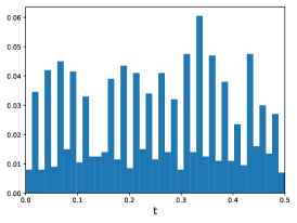
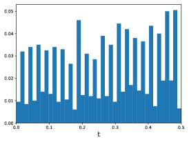
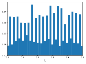
Figure 11: Temporal density of the 1st, 3rd, 5th adaptivity iteration. ($\beta=1000$, Galerkin projection)

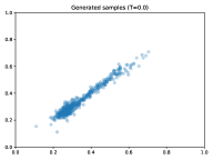
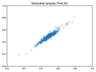
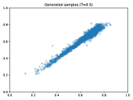
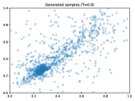
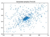
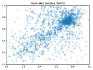
Figure 12: The distribution of collocation points obtained by bounded KRnet $p_{\mathrm{B-KRnet}}(x|t)$ for the first and last updates. From left to right: $t=0,0.25$ and $0.5$. ($\beta=1000,$ Galerkin projection)

5 Conclusion

In this paper we have developed a hybrid numerical method for solving evolution partial differential equations (PDEs) by merging the time finite element method with deep neural networks. The key idea of the proposed method is to represent the solution as a tensor product comprising a series of predetermined local finite element basis functions in time and a sequence of unspecified neural networks in space. Subsequently, we apply the Galerkin or collocation formulation to the original evolution equation, eliminating the temporal variable and resulting in a differential system exclusively involving unknown neural networks with respect to the spatial variable. Furthermore, to address the evolution problems characterized by high dimensionality and low regularity, we have developed an adaptive sampling strategy where the training set and the model are updated alternately to improve both efficiency and accuracy. Numerical experiments have demonstrated the effectiveness of our proposed approaches. Several issues deserve further investigation. First, a rigorous error analysis is still missing especially for the collocation projection. Second, while herein we only consider linear and quadratic finite element methods over a uniform mesh, the strategy can also be generalized to $hp$-finite element method in the temporal domain. Finally, the proposed methods need to be further investigated for convection-dominated problems.

Appendix A Exact periodic boundary conditions

Following the work from [10, 11], we can exactly enforce $C^{\infty}$ periodic boundary conditions by applying a Fourier feature encoding to the spatial input of the network. The spatial encoding is

$$v(x)=\left\{1,\cos(\omega x),\sin(\omega x),\cdots,\cos(M\omega x),\sin(M\omega x)\right\}$$

where $\omega=\frac{2\pi}{L},L=x_{\mathrm{max}}-x_{\mathrm{min}}$, and $M$ is a non-negative integer representing the sinusoidal frequency of the input. In this work, we take $M=10.$

Appendix B Supplementary Figures

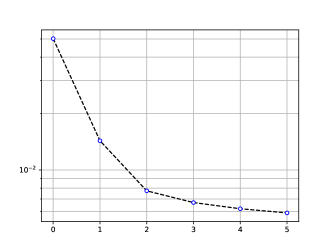
Figure 13: Relative $L_{2}$ error of different adaptivity iterations for Galerkin projection. ($\beta=200$)

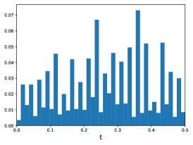
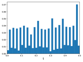
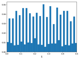
Figure 14: Temporal weights $\lambda_{i}$ of the 1st, 3rd, 5th adaptivity iteration. ($\beta=200$, Galerkin projection)

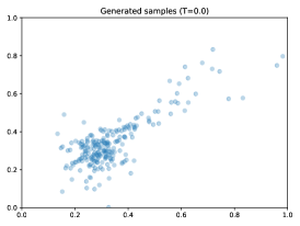
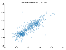
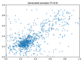
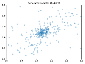
Figure 15: From top to bottom: The generated samples of the first, and the last adaptivity iteration. ($\beta=200$, Galerkin projection)

References

• Weinan [2021] E. Weinan, The dawning of a new era in applied mathematics, Notices of the American Mathematical Society 68 (2021) 565–571.
• Han et al. [2018] J. Han, A. Jentzen, W. E, Solving high-dimensional partial differential equations using deep learning, Proceedings of the National Academy of Sciences 115 (2018) 8505–8510.
• Karniadakis et al. [2021] G. E. Karniadakis, I. G. Kevrekidis, L. Lu, P. Perdikaris, S. Wang, L. Yang, Physics-informed machine learning, Nature Reviews Physics 3 (2021) 422–440.
• Raissi et al. [2019] M. Raissi, P. Perdikaris, G. E. Karniadakis, Physics-informed neural networks: A deep learning framework for solving forward and inverse problems involving nonlinear partial differential equations, Journal of Computational physics 378 (2019) 686–707.
• Weinan and Yu [2018] E. Weinan, B. Yu, The deep Ritz method: A deep learning-based numerical algorithm for solving variational problems, Communications in Mathematics and Statistics 6 (2018) 1–12.
• Zang et al. [2020] Y. Zang, G. Bao, X. Ye, H. Zhou, Weak adversarial networks for high-dimensional partial differential equations, Journal of Computational Physics 411 (2020) 109409.
• Wight and Zhao [2020] C. L. Wight, J. Zhao, Solving Allen-Cahn and Cahn-Hilliard equations using the adaptive physics informed neural networks, arXiv preprint arXiv:2007.04542 (2020).
• Krishnapriyan et al. [2021] A. Krishnapriyan, A. Gholami, S. Zhe, R. Kirby, M. W. Mahoney, Characterizing possible failure modes in physics-informed neural networks, Advances in Neural Information Processing Systems 34 (2021) 26548–26560.
• Mattey and Ghosh [2022] R. Mattey, S. Ghosh, A novel sequential method to train physics informed neural networks for allen cahn and cahn hilliard equations, Computer Methods in Applied Mechanics and Engineering 390 (2022) 114474.
• Wang et al. [2024] S. Wang, S. Sankaran, P. Perdikaris, Respecting causality for training physics-informed neural networks, Computer Methods in Applied Mechanics and Engineering 421 (2024) 116813.
• Penwarden et al. [2023] M. Penwarden, A. D. Jagtap, S. Zhe, G. E. Karniadakis, R. M. Kirby, A unified scalable framework for causal sweeping strategies for Physics-Informed Neural Networks (PINNs) and their temporal decompositions, arXiv preprint arXiv:2302.14227 (2023).
• Du and Zaki [2021] Y. Du, T. A. Zaki, Evolutional deep neural network, Physical Review E 104 (2021) 045303.
• Bruna et al. [2022] J. Bruna, B. Peherstorfer, E. Vanden-Eijnden, Neural galerkin scheme with active learning for high-dimensional evolution equations, arXiv preprint arXiv:2203.01360 (2022).
• Schwerdtner et al. [2023] P. Schwerdtner, P. Schulze, J. Berman, B. Peherstorfer, Nonlinear embeddings for conserving hamiltonians and other quantities with neural galerkin schemes, arXiv preprint arXiv:2310.07485 (2023).
• Kao et al. [2024] T. Kao, J. Zhao, L. Zhang, petnns: Partial evolutionary tensor neural networks for solving time-dependent partial differential equations, arXiv preprint arXiv:2403.06084 (2024).
• Berman and Peherstorfer [2024] J. Berman, B. Peherstorfer, Randomized sparse neural galerkin schemes for solving evolution equations with deep networks, Advances in Neural Information Processing Systems 36 (2024).
• Wang et al. [2021] S. Wang, H. Wang, P. Perdikaris, Learning the solution operator of parametric partial differential equations with physics-informed deeponets, Science advances 7 (2021) eabi8605.
• Wang and Perdikaris [2023] S. Wang, P. Perdikaris, Long-time integration of parametric evolution equations with physics-informed deeponets, Journal of Computational Physics 475 (2023) 111855.
• Geneva and Zabaras [2020] N. Geneva, N. Zabaras, Modeling the dynamics of pde systems with physics-constrained deep auto-regressive networks, Journal of Computational Physics 403 (2020) 109056.
• Geneva and Zabaras [2022] N. Geneva, N. Zabaras, Transformers for modeling physical systems, Neural Networks 146 (2022) 272–289.
• Bruno et al. [2022] O. P. Bruno, J. S. Hesthaven, D. V. Leibovici, FC-based shock-dynamics solver with neural-network localized artificial-viscosity assignment, Journal of Computational Physics: X 15 (2022) 100110.
• Dresdner et al. [2022] G. Dresdner, D. Kochkov, P. Norgaard, L. Zepeda-Núñez, J. A. Smith, M. P. Brenner, S. Hoyer, Learning to correct spectral methods for simulating turbulent flows, arXiv preprint arXiv:2207.00556 (2022).
• Chiu et al. [2022] P.-H. Chiu, J. C. Wong, C. Ooi, M. H. Dao, Y.-S. Ong, CAN-PINN: A fast physics-informed neural network based on coupled-automatic–numerical differentiation method, Computer Methods in Applied Mechanics and Engineering 395 (2022) 114909.
• Gu and Ng [2022] Y. Gu, M. K. Ng, Deep adaptive basis Galerkin method for high-dimensional evolution equations with oscillatory solutions, SIAM Journal on Scientific Computing 44 (2022) A3130–A3157.
• Griewank and Walther [2008] A. Griewank, A. Walther, Evaluating derivatives: principles and techniques of algorithmic differentiation, SIAM, 2008.
• Douglas and Dupont [1973] J. Douglas, T. Dupont, A finite element collocation method for quasilinear parabolic equations, mathematics of computation 27 (1973) 17–28.
• Percell and Wheeler [1980] P. Percell, M. F. Wheeler, A $C^{1}$ finite element collocation method for elliptic equations, SIAM Journal on Numerical Analysis 17 (1980) 605–622.
• Boor and Swartz [1973] C. d. Boor, B. Swartz, Collocation at Guass points, SIAM Journal on Numerical Analysis 10 (1973) 582–606.
• Tang et al. [2023] K. Tang, X. Wan, C. Yang, DAS-PINNs: A deep adaptive sampling method for solving high-dimensional partial differential equations, Journal of Computational Physics 476 (2023) 111868.
• Gao et al. [2023] Z. Gao, L. Yan, T. Zhou, Failure-informed adaptive sampling for PINNs, SIAM Journal on Scientific Computing 45 (2023) A1971–A1994.
• Müller et al. [2019] T. Müller, B. McWilliams, F. Rousselle, M. Gross, J. Novák, Neural importance sampling, ACM Transactions on Graphics (ToG) 38 (2019) 1–19.
• Zeng et al. [2023] L. Zeng, X. Wan, T. Zhou, Bounded KRnet and its applications to density estimation and approximation, arXiv preprint arXiv:2305.09063 (2023).
• Carlier et al. [2010] G. Carlier, A. Galichon, F. Santambrogio, From Knothe’s transport to Brenier’s map and a continuation method for optimal transport, SIAM Journal on Mathematical Analysis 41 (2010) 2554–2576.
• Dinh et al. [2016] L. Dinh, J. Sohl-Dickstein, S. Bengio, Density estimation using real nvp, arXiv preprint arXiv:1605.08803 (2016).
• Feng et al. [2022] X. Feng, L. Zeng, T. Zhou, Solving time dependent Fokker-Planck equations via temporal normalizing flow, Communications in Computational Physics 32 (2022) 401–423.
• Glorot and Bengio [2010] X. Glorot, Y. Bengio, Understanding the difficulty of training deep feedforward neural networks, in: Proceedings of the thirteenth international conference on artificial intelligence and statistics, JMLR Workshop and Conference Proceedings, pp. 249–256.
• Kingma and Ba [2014] D. P. Kingma, J. Ba, Adam: A method for stochastic optimization, arXiv preprint arXiv:1412.6980 (2014).
• Bradbury et al. [2018] J. Bradbury, R. Frostig, P. Hawkins, M. J. Johnson, C. Leary, D. Maclaurin, G. Necula, A. Paszke, J. VanderPlas, S. Wanderman-Milne, et al., Jax: composable transformations of python+ numpy programs (2018).