The Interaction of Moving $\mathbf{Q\bar{Q}}$ and QQq in the Thermal Plasma

Abstract

The strength of the force between heavy quarks is studied for heavy quarkonium ($\mathrm{Q\bar{Q}}$) and doubly heavy baryons ($\mathrm{QQq}$) at finite temperature and rapidity using the gauge/gravity duality in this paper. The strength of the interaction is defined as an effective running coupling $\alpha$ from lattice. By considering the $\mathrm{Q\bar{Q}}$ and $\mathrm{QQq}$ moving through the thermal quark-gluon plasma, we find that the interaction of heavy quarks for $\mathrm{Q\bar{Q}}$ is small and remains almost constant when $L<0.2\,\mathrm{fm}$. The strength of the interaction for $\mathrm{QQq}$ is always less than that for $\mathrm{Q\bar{Q}}$ and approaches a constant when $L<0.4\,\mathrm{fm}$. The $\alpha$ and the maximum of effective running coupling $\tilde{\alpha}$ for both $\mathrm{Q\bar{Q}}$ and $\mathrm{QQq}$ decrease with increasing temperature or rapidity. Through comparison, we find that $\mathrm{QQq}$ is more sensitive to changes in temperature and rapidity, and the interaction force between quarks is always less than that of $\mathrm{Q\bar{Q}}$, indicating that $\mathrm{Q\bar{Q}}$ is more stable than $\mathrm{QQq}$ in the presence of temperature and rapidity.

I Introduction

The running coupling constant serves as a crucial metric for measuring the strength of the strong interaction between quarks, and the force between quarks is essential for our understanding of $\mathrm{QCD}$ and the $\mathrm{QCD}$ phase transition. When quarks are confined within hadrons, the force between them increases with the separation distance until the string breaks, resulting in the creation of new quark-antiquark pairs, thereby preventing the isolation of free quarks. $\mathrm{QCD}$ predicts that deconfinement occurs under extreme conditions, where color screening happens at long distances between quarks, leading to the emergence of relatively free quarks Matsui and Satz (1986); Kharzeev and Satz (1995); Witten (1998a). A system composed of such deconfined particles is referred to as a Quark-Gluon Plasma ($\mathrm{QGP}$) Gyulassy and McLerran (2005); Jacobs and Wang (2005). Moreover, the property of asymptotic freedom indicates that quarks behave as free particles at very high energy scales. These phenomena can be attempted to be explained through the running of the coupling constant. Additionally, the running coupling constant plays a key role in many important physical processes such as jet quenching, heavy quarkonium production, and Higgs particle production Carcamo Hernandez et al. (2014). Lattice QCD defined an effective running coupling Kaczmarek et al. (2004); Kaczmarek and Zantow (2005); Kaczmarek (2007); Bazavov et al. (2018),

$$\alpha_{Q\bar{Q}}(r)=\frac{1}{C_{F}}r^{2}\frac{\partial E(r)}{\partial r},$$ (1)

to study the force between the static quark and antiquark. $C_{F}=4/3$ is the Casimir operator in the fundamental representation of $\mathrm{SU}(3)$ and $E$ is the static energy of $\mathrm{Q\bar{Q}}$.

Creating $\mathrm{QGP}$ through heavy-ion collisions allows for the simulation of the extreme conditions of high temperature and rapid expansion present in the early universe Laine (2006); Asaka et al. (2006); Hindmarsh and Philipsen (2005); Rothkopf (2020, 2020). This helps us to understand the evolution of the early universe and the properties of $\mathrm{QCD}$. Heavy quarkonium is an important probe for studying conditions of extreme high temperature and rapid expansion. Moreover, in the recent $\mathrm{LHCb}$ experiment at $\mathrm{CERN}$, researchers have discovered a new particle known as $\Xi_{cc}^{++}$ Aaij et al. (2017, 2018). It is composed of two heavy quarks and one light quark, and its discovery has greatly increased interest in the study of doubly heavy baryon. The running coupling constant has been extensively studied in the Refs. Giunti et al. (1991); Baikov et al. (2017); Javidan et al. (2021); Aguilar et al. (2002); Lombardo and Mazzitelli (1997); Zhou et al. (2023); Bloch et al. (2004); Deur et al. (2016); Yu et al. (2022); Takaura et al. (2019); Chen et al. (2022a), as discussed through lattice calculations at finite temperatures in the Refs. Kaczmarek (2009); Kaczmarek et al. (2004); Kaczmarek and Zantow (2005). It is well known that the $\mathrm{QGP}$ has been rapidly expanding since its inception. Therefore, rapidity is an unavoidable factor to consider when discussing the effective running coupling of particles. This paper attempts to reveal more information about the $\mathrm{QGP}$ by contrasting heavy quarkonium and doubly heavy baryon at finite temperatures and rapidities. This can aid in our understanding of particle transport in the $\mathrm{QGP}$ and the plasma’s effect on particle properties. Moreover, the interaction forces between quarks in the $\mathrm{QGP}$ can also reflect the state of the $\mathrm{QGP}$ to a certain extent, such as determining whether it is a strongly coupled $\mathrm{QGP}$ ($\mathrm{sQGP}$) or a weakly coupled $\mathrm{QGP}$ ($\mathrm{wQGP}$) Nijs et al. (2023); Shuryak (2017); Arnold et al. (2005).

Lattice gauge theory remains the fundamental tool for studying non-perturbative phenomena in $\mathrm{QCD}$, yet its application to doubly heavy baryon has been relatively limited Yamamoto et al. (2008a); Najjar and Bali (2009). Gauge/gravity duality offers a new avenue for probing strongly coupled gauge theories. Originally, Maldacena Maldacena (1998) proposed the gauge/gravity duality for conformal field theories, but it was subsequently extended to encompass theories akin to $\mathrm{QCD}$, thereby establishing to some extent a linkage between string theory and heavy-ion collisions Aharony et al. (2000); Casalderrey-Solana et al. (2014); Gubser (2013). Research on moving heavy quarkonium can be found in lattice Thakur et al. (2017), effective field theory Escobedo et al. (2013), perturbative QCD Song et al. (2008), S matrix Benzahra (2004), and holographic QCD Liu et al. (2007); Chen et al. (2021, 2018); Finazzo and Noronha (2015); Ali-Akbari et al. (2014); Andreev (2022a); Krishnan (2008); Chernicoff et al. (2013); Bitaghsir Fadafan and Tabatabaei (2016); Zhou et al. (2020); Feng et al. (2020); Zhou et al. (2021). Moreover, the multi-quark potential obtained through effective string model is in good agreement with lattice results Alexandrou et al. (2002, 2003); Takahashi et al. (2002); Andreev (2021a, 2016a, 2016b, 2020a, b, 2023a, 2022b, 2023b); Mei et al. (2023); Andreev (2022c); Mei et al. (2024).

In this paper, we primarily investigate the effective running coupling of heavy quarkonium and doubly heavy baryon at finite temperature and rapidity. The rest of the paper is organized as follows: in the Sec. II, we determine the holographic parameters by fitting their lattice potentials, and present the state diagram of particles in the $T-\eta$ plane. In the Sec. III, we discuss the effective running coupling of heavy quarkonium and doubly heavy baryon, including the effective running coupling with distance, and with temperature and rapidity, as well as the impact of rapidity on the temperature dependence of the effective coupling constant. Additionally, we examine the effects of temperature and rapidity on their screening distances. In the Sec. IV, we provide a summary of this paper.

II Preliminaries

The effective string holographic models have been proposed by Andreev recently. These models can not only describe the potential of heavy quarkonium Andreev and Zakharov (2007), but also describe the potential of exotic hadrons Andreev (2016b, a, 2008, 2024, 2023a, 2023b); Chen et al. (2022b). The purpose of this study is to reveal the properties of QQ and QQq based on the effective string model by investigating the effective running coupling and the screening distance of their motion in a thermal medium. First, we present the metric

$$ds^{2} =w(r)\Big{(}-f(r)dt^{2}+d\vec{x}^{2}+\frac{1}{f(r)}dr^{2}\Big{)}+e^{-\mathbf{s}r^{2}}g_{ab}^{(5)}d\omega^{a}d\omega^{b},$$ (2)

where

$$w(r) =\frac{e^{\mathbf{s}r^{2}}R^{2}}{r^{2}}\,,$$ (3)

$$f(r) =1-\frac{r^{4}}{r_{h}^{4}}.$$

The metric signifies a deformation of the Euclidean $\mathrm{AdS_{5}}\times\mathrm{S_{5}}$ space, controlled by a single parameter $\mathbf{s}$ and with a radius $R=1$. In this work, $\mathbf{s}$ is determined to be $0.41\,\mathrm{GeV^{2}}$ by fitting the lattice potential of heavy quarkonium. Therefore, the metric is composed of an $\mathrm{AdS_{5}}$ space and a five-dimensional compact space $\mathrm{X}$ with coordinates $\omega^{a}$. The function $f(r)$ is the blackening factor, which decreases within the interval $[0,r_{h}]$, where $r_{h}$ represents the black hole horizon (brane). Additionally, when hadrons are confined, an imaginary wall exists at $r_{w}$ on the $r$-axis Wen et al. (2024); Liang et al. (2023); Cao et al. (2022, 2023); Yang and Yuan (2015); Andreev and Zakharov (2007); Colangelo et al. (2011). The Hawking temperature $T$ associated with the black hole is given by:

$$T=\frac{1}{4\pi}{\left|\frac{df}{dr}\right|}_{r=r_{h}}=\frac{1}{\pi r_{h}}.$$ (4)

In this paper, we consider a particle moving at a rapidity $\eta$ along the $x_{3}$ direction in a thermal medium at temperature $T$. It is known that the particle is also subject to drag force in the medium, but this is not the main focus of our discussion Andreev (2018a, b). We can assume that the particle is at rest, while the thermal medium moves relative to it at rapidity $\eta$, which can be considered as a ”thermal wind” blowing past the particle in the $x_{3}$ direction Liu et al. (2007); Finazzo and Noronha (2015); Chen et al. (2018); Andreev (2022a); Thakur et al. (2017). Through a Lorentz transformation, we can provide a new background metric:

$$ds^{2}=w(r) \Big{(}-g_{1}(r)dt^{2}-2\sinh(\eta)\cosh(\eta)\big{(}1-\frac{g_{1}(r)}{g_{2}(r)}\big{)}dx_{3}dt$$

$$+g_{3}(r)dx_{3}^{2}+dx_{1}^{2}+dx_{2}^{2}+\frac{g_{2}(r)}{g_{1}(r)}dr^{2}\Big{)}+e^{-\mathbf{s}r^{2}}g_{ab}^{(5)}d\omega^{a}d\omega^{b},$$ (5)

where

$$g_{1}(r) =f(r)\cosh^{2}(\eta)-\sinh^{2}(\eta),$$ (6)

$$g_{2}(r) =\frac{g_{1}(r)}{f(r)},$$

$$g_{3}(r) =\cosh^{2}(\eta)-f(r)\sinh^{2}(\eta).$$

The Nambu-Goto action of a string is

$$S_{NG}=-g\int d\xi^{0}d\xi^{1}\sqrt{-\det g_{ab}},$$ (7)

where the $g_{ab}$ is an induced metric ($\xi^{0}$, $\xi^{1}$) are worldsheet coordinates, and $g$ is related to the string tension. Based on the $\mathrm{AdS/CFT}$ correspondence, we know that the vertex corresponds to a five brane Witten (1998b); Gukov et al. (1998), the baryon vertex action is $S_{vert}=\tau_{5}\int d^{6}\xi\sqrt{\gamma^{(6)}}$, where $\tau_{5}$ is the brane tension and $\xi^{i}$ are the world-volume coordinates. Since the brane is wrapped on the compact space $\mathrm{X}$, it appears point-like in $\mathrm{AdS_{5}}$. We choose a static gauge where $\xi^{0}=t$ and $\xi^{a}=\theta^{a}$, with $\theta^{a}$ being the coordinates on $\mathrm{X}$. Consequently, the action is:

$$S_{vert}=\tau_{v}\int dt\frac{e^{-2\mathbf{s}r^{2}}}{r}\sqrt{g_{1}(r)},$$ (8)

where $\tau_{v}$ is a dimensionless parameter defined by $\tau_{v}=\mathrm{\tau}_{5}R\mathrm{vol(X)}$ and $\mathrm{vol(X)}$ is a volume of $\mathrm{X}$. Finally, we consider the light quarks at the endpoints of the string as a tachyon field, which is coupled to the worldsheet boundary through $S_{q}=\int d\tau\mathbf{e}\mathrm{T}$, where $\mathrm{T}(x,r)$ is a scalar field that describes open string tachyon, $\tau$ is a coordinate on the boundary, and $\mathbf{e}$ is the boundary metric Andreev (2020b); Erlich et al. (2005). We consider only the case where $\mathrm{T}(x,r)=\mathrm{T_{0}}$ and the worldsheet boundary is a line in the $t$ direction, in which case the action can be written as:

$$S_{q}=m\int dt\frac{e^{\frac{\mathbf{s}r^{2}}{2}}}{r}\sqrt{g_{1}(r)},$$ (9)

This action represents a particle of mass $\mathrm{T_{0}}$ at rest, with a medium at temperature $T$ moving past it at a rapidity $\eta$.

II.1 The potential and effective running coupling of heavy quarkonium

In this paper, we investigate the scenario where the direction of motion is perpendicular to the heavy quark pair, with the heavy quark pair located at $x_{1}$ and the rapidity $\eta$ along the $x_{3}$ direction. For brevity, $x$ will be used to denote $x_{1}$ in the following. Then we choose the static gauge $\xi^{0}=t$, $\xi^{1}=x$, and the action of $\mathrm{Q\bar{Q}}$ can be written as:

$$S_{\mathrm{Q\bar{Q}}} =g_{\mathrm{Q\bar{Q}}}\int_{0}^{t}\int_{-\frac{L}{2}}^{\frac{L}{2}}w(r)\sqrt{g_{1}(r)+g_{2}(r)(\partial_{x}r)^{2}}dx$$ (10)

$$=g_{\mathrm{Q\bar{Q}}}t\int_{-\frac{L}{2}}^{\frac{L}{2}}w(r)\sqrt{g_{1}(r)+g_{2}(r)(\partial_{x}r)^{2}}dx,$$ (11)

where the $g_{\mathrm{Q\bar{Q}}}=0.176$. And the boundary condition of $r(x)$ is

$$r\Big{(}\pm\,\frac{L}{2}\Big{)}=0,\,r(0)=r_{0},\,(\partial_{x}r|_{r=r_{0}})^{2}=0.$$ (12)

By substituting into the Euler-Lagrange equation, we can obtain:

$$\partial_{x}r=\sqrt{\frac{w(r)^{2}g_{1}(r)^{2}-g_{1}(r)w(r_{0})^{2}g_{1}(r_{0})}{w(r_{0})^{2}g_{1}(r_{0})g_{2}(r)}}.$$ (13)

The distance between heavy quark and anti-quark is:

$$L=2\int_{0}^{r_{0}}\partial_{r}xdr,$$ (14)

where $\partial_{r}x=\frac{\partial x}{\partial r}=\frac{1}{\partial_{x}r}$. By $E=S/t$ and after normalizing, we can obtain the potential of $\mathrm{Q\bar{Q}}$,

$$E_{\mathrm{Q\bar{Q}}}=2g_{\mathrm{Q\bar{Q}}}\Big{(}\int_{0}^{r_{0}}\big{(}w(r)\sqrt{g_{1}(r)(\partial_{r}x)^{2}+g_{2}(r)}-\frac{1}{r^{2}}\big{)}dr-\frac{1}{r_{0}}\Big{)}.$$ (15)

We consider the pattern of $\mathrm{Q\bar{Q}}$ string breaking as

$$\mathrm{Q\bar{Q}}\longrightarrow\mathrm{Q\bar{q}}+\mathrm{\bar{Q}q}.$$ (16)

It is easy to know that

$$E_{break}=E_{\mathrm{Q\bar{q}}}+E_{\mathrm{\bar{Q}q}}=2g_{\mathrm{Q\bar{Q}}}\Big{(}\int_{0}^{r_{q}}\big{(}w(r)\sqrt{g_{2}(r)}-\frac{1}{r^{2}}\big{)}dr-\frac{1}{r_{q}}+n\frac{e^{\frac{sr_{q}^{2}}{2}}}{r_{q}}\sqrt{g_{1}(r_{q})}\Big{)}.$$ (17)

At $T=0,\eta=0$, we obtain $E_{break}=1.057\mathrm{GeV}$ which means that string breaking occurs for the $\mathrm{Q\bar{Q}}$ at $E_{\mathrm{Q\bar{Q}}}=1.057\mathrm{GeV}$, resulting in a breaking distance of $L_{break}=1.23\mathrm{fm}$. We present a comparison between the potential obtained by the model and the lattice potential in Fig. 1.

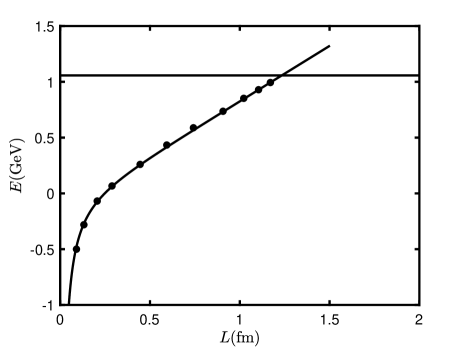
Figure 1: The black curve represents the $\mathrm{Q\bar{Q}}$ potential at $T=0,\eta=0$, while the straight line represents the potential after string breaking. The black solid dot represents the lattice data from quenched QCD Kaczmarek et al. (2004).

Therefore, the effective running coupling of $\mathrm{Q\bar{Q}}$ from lattice QCD is given by Kaczmarek et al. (2004); Kaczmarek and Zantow (2005); Kaczmarek (2007); Bazavov et al. (2018)

$$\alpha_{\mathrm{Q\bar{Q}}}=\frac{3L^{2}}{4}\frac{dE_{\mathrm{Q\bar{Q}}}}{dL}.$$ (18)

Then we present its basic behavior in Fig. 2. The effective coupling constant of $\mathrm{Q\bar{Q}}$ is very small and increases only slightly at small scales when $L<0.2\,\mathrm{fm}$, which can explain the phenomenon of asymptotic freedom exhibited by quarks at short distances. At larger scales, the obvious increase of the effective coupling constant with distance also corresponds to our understanding of the strong interaction force. We discuss in detail its effective running coupling properties in moving thermal media in the subsequent sections.

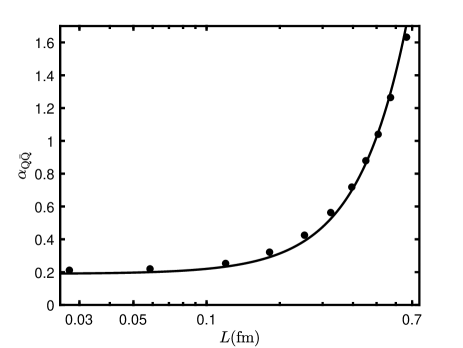
Figure 2: The effective running coupling of $\mathrm{Q\bar{Q}}$ at $T=0,\eta=0$. The black solid dot represents the lattice data from quenched QCD Kaczmarek et al. (2004).

II.2 The potential and effective running coupling of doubly heavy baryon

The double heavy baryon consists of two heavy quarks and one light quark, which introduces a baryon vertex. When considering a string configuration for the ground state of $\mathrm{QQq}$, it is natural due to symmetry to place the light quark between the two heavy quarks Andreev (2021a). The $\mathrm{QQq}$ potential depends only on the distance $L$ between the heavy quarks. In the Ref. Yamamoto et al. (2008a), the $\mathrm{QQq}$ potential is also fitted to a function similar to the Cornell potential:

$$E_{\mathrm{QQq}}=\sigma_{eff}L-\frac{A_{eff}}{L}+C_{eff},$$ (19)

where the first term represents the confinement potential, and the second term comes from one-gluon exchange Yamamoto et al. (2008a). Due to the octet nature of gluons, the factor $4/3$ is included in $A_{eff}$. As the distance between the heavy quark pair increases, its string configuration will change, as shown in Fig. 3. And the three configurations from left to right are called: small $L$, intermediate $L$, and large $L$. In the small $L$ configuration, the action is composed of three strings, the baryon vertex, and the light quark. After $r_{v}=r_{q}$, it transitions to the intermediate $L$ configuration, where the position of the light quark coincides with the baryon vertex, and the action is constituted by two strings, the baryon vertex, and the light quark. When the string at the baryon vertex transitions from a ”convex” to a ”concave” shape, it becomes the large $L$ configuration. At this configuration, the composition of the action is consistent with the intermediate $L$. Therefore, the total action at small $L$ is:

$$S=\sum_{i=1}^{3}S_{NG}^{(i)}+S_{vert}+S_{q}.$$ (20)

Then we choose the static gauge where $\xi^{0}=t,\,\xi^{1}=r$, and the boundary conditions of $x(r)$ is:

$$x(0)=\pm\,\frac{L}{2},\,x(r_{v})=x(r_{q})=0,\,\begin{cases}(\partial_{r}x)^{2}=\cot^{2}(\alpha),&r=r_{v}\\ (\partial_{r}x)^{2}=0,&r\in(r_{v},r_{q}].\end{cases}$$ (21)

And we obtain the total action as

$$S=g_{\mathrm{QQq}}t \Big{(}2\int_{0}^{r_{v}}w(r)\sqrt{g_{1}(r)(\partial_{r}x)^{2}+g_{2}(r)}dr+\int_{r_{v}}^{r_{q}}w(r)\sqrt{g_{2}(r)}dr$$

$$+3k\frac{e^{-2\mathbf{s}r^{2}}}{r}\sqrt{g_{1}(r)}+n\frac{e^{\frac{\mathbf{s}r^{2}}{2}}}{r}\sqrt{g_{1}(r)}\Big{)},$$ (22)

where $k=\frac{\tau_{v}}{3g_{\mathrm{QQq}}},n=\frac{m}{g_{\mathrm{QQq}}}$. By substituting the first term of the action into the Euler-Lagrange equation, we obtain

$$\partial_{r}x=\sqrt{\frac{w(r_{v})^{2}g_{1}(r_{v})^{2}g_{2}(r)}{w(r)^{2}g_{1}(r)^{2}\big{(}g_{1}(r_{v})+g_{2}(r_{v})\tan^{2}(\alpha)\big{)}-g_{1}(r)w(r_{v})^{2}g_{1}(r_{v})^{2}}}.$$ (23)

Furthermore, there must be a balance of forces at the light quark and the baryon vertex, with the light quark site satisfying $f_{q}+e_{3}^{\prime}=0$, and the vertex site satisfying $f_{v}+e_{3}+e_{1}+e_{2}=0$. These forces are obtained by taking the variation of their action:

$$e_{1} =g_{\mathrm{QQq}}w(r_{v})\Big{(}-\sqrt{\frac{g_{1}(r_{v})f(r_{v})}{f(r_{v})+\tan^{2}\alpha}},\,-\sqrt{\frac{g_{1}(r_{v})}{f(r_{v})^{2}\cot^{2}(\alpha)+f(r_{v})}}\Big{)},$$ (24)

$$e_{2} =g_{\mathrm{QQq}}w(r_{v})\Big{(}\sqrt{\frac{g_{1}(r_{v})f(r_{v})}{f(r_{v})+\tan^{2}\alpha}},\,-\sqrt{\frac{g_{1}(r_{v})}{f(r_{v})^{2}\cot^{2}(\alpha)+f(r_{v})}}\Big{)},$$ (25)

$$e_{3} =g_{\mathrm{QQq}}w(r_{v})\big{(}0,\,\sqrt{g_{2}(r_{v})}\big{)},$$ (26)

$$e_{3}^{\prime} =g_{\mathrm{QQq}}w(r_{q})\big{(}0,\,-\sqrt{g_{2}(r_{q})}\big{)},$$ (27)

$$f_{q} =\Big{(}0,\,-g_{\mathrm{QQq}}n\partial_{r_{q}}\big{(}\frac{e^{\frac{\mathbf{s}r_{q}^{2}}{2}}}{r_{q}}\sqrt{g_{1}(r_{q})}\big{)}\Big{)},$$ (28)

$$f_{v} =\Big{(}0,\,-3g_{\mathrm{QQq}}k\partial_{r_{v}}\big{(}\frac{e^{-2\mathbf{s}r_{v}^{2}}}{r_{v}}\sqrt{g_{1}(r_{v})}\big{)}\Big{)},$$ (29)

it is evident that when $T$ and $\eta$ are fixed, the force at the light quark site depends only on $r_{q}$, while the force at the vertex involves only two unknowns, $r_{v}$ and $\alpha$. Therefore, we can determine the value of $r_{q}$ and the function of $\alpha$ in terms of $r_{v}$, and from these, we can derive the potential of small $L$. The potential, with the divergent terms eliminated through normalization, is represented as:

$$E_{small}=g_{\mathrm{QQq}} \Big{(}2\int_{0}^{r_{v}}\big{(}w(r)\sqrt{g_{1}(r)(\partial_{r}x)^{2}+g_{2}(r)}-\frac{1}{r^{2}}\big{)}dr-\frac{2}{r_{v}}+\int_{r_{v}}^{r_{q}}w(r)\sqrt{g_{2}(r)}dr$$

$$+3k\frac{e^{-2\mathbf{s}r_{v}^{2}}}{r_{v}}\sqrt{g_{1}(r_{v})}+n\frac{e^{\frac{\mathbf{s}r_{q}^{2}}{2}}}{r_{q}}\sqrt{g_{1}(r_{q})}\Big{)}+c.$$ (30)

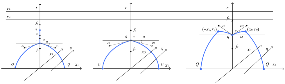
Figure 3: String structure of the double heavy baryon (distance $L$ increases from left to right). The heavy quark pair is located in the $x_{1}$ direction, while the baryon vertex $\mathrm{v}$ and the light quark $\mathrm{q}$ are on the $r$-axis. The rapidity $\eta$ is along the $x_{3}$-axis direction. The heavy quark, light quark, and baryon vertex are connected by blue strings. The black arrows represent forces. $r_{h}$ is the position of the black hole horizon. $r_{w}$ is the position of an imaginary wall when the $\mathrm{QQq}$ is confined.

At intermediate $L$, the total action is given by

$$S=\sum_{i=1}^{2}S_{NG}^{(i)}+S_{vert}+S_{q},$$ (31)

and the boundary conditions of $x(r)$ become

$$x(0)=\pm\,\frac{L}{2},\,x(r_{v})=0,\,(\partial_{r}x|_{r=r_{v}})^{2}=\cot^{2}(\alpha).$$ (32)

And only the forces at the vertices need to be considered: $f_{v}+f_{q}+e_{1}+e_{2}=0$, Since $r_{q}=r_{v}$, we only need to replace $r_{q}$ with $r_{v}$ in the force. Similarly, we can obtain its potential at intermediate $L$ as:

$$E_{intermediate}=g_{\mathrm{QQq}} \Big{(}2\int_{0}^{r_{v}}\big{(}w(r)\sqrt{g_{1}(r)(\partial_{r}x)^{2}+g_{2}(r)}-\frac{1}{r^{2}}\big{)}dr-\frac{2}{r_{v}}$$

$$+3k\frac{e^{-2\mathbf{s}r_{v}^{2}}}{r_{v}}\sqrt{g_{1}(r_{v})}+n\frac{e^{\frac{\mathbf{s}r_{v}^{2}}{2}}}{r_{v}}\sqrt{g_{1}(r_{v})}\Big{)}+c.$$ (33)

The distance between heavy quark pairs for small $L$ and intermediate $L$ is calculated using the following function

$$L=2\int_{0}^{r_{v}}\partial_{r}xdr.$$ (34)

As Fig. 3 shows the large $L$ is special because the string has two additional smooth inflection points. For the string configuration at large $L$, we choose a new metric $\xi^{0}=t,\,\xi^{1}=x$, and now the boundary condition of $r(x)$ is

$$r\Big{(}\pm\,\frac{L}{2}\Big{)}=0,\,r(0)=r_{v},\,\,\begin{cases}(\partial_{x}r)^{2}=\tan^{2}(\alpha),&r=r_{v}\\ (\partial_{x}r)^{2}=0,&r=r_{0}.\end{cases}$$ (35)

For configurations at large $L$, the form of the force balance equation at the vertex remains consistent with that at intermediate $L$ but introduces an additional unknown $r_{0}$, which can be determined through the properties of the first integral

$$\mathcal{H}|_{r=r_{0}} =w(r_{0})\sqrt{g_{1}(r_{0})},$$ (36)

$$\mathcal{H}|_{r=r_{v}} =\frac{w(r_{v})g_{1}(r_{v})}{\sqrt{g_{1}(r_{v})+g_{2}(r_{v})\tan^{2}(\alpha)}},$$ (37)

$$w(r_{0})\sqrt{g_{1}(r_{0})} =\frac{w(r_{v})g_{1}(r_{v})}{\sqrt{g_{1}(r_{v})+g_{2}(r_{v})\tan^{2}(\alpha)}}.$$ (38)

Furthermore we obtain

$$\partial_{x}r=\sqrt{\frac{w(r)^{2}g_{1}(r)^{2}-g_{1}(r)w(r_{0})^{2}g_{1}(r_{0})}{w(r_{0})^{2}g_{1}(r_{0})g_{2}(r)}}.$$ (39)

For convenience in the calculation, we present the potential after equivalent transformation and normalization as follows

$$E_{large}=g_{\mathrm{QQq}} \Big{(}2\int_{0}^{r_{v}}\big{(}w(r)\sqrt{g_{1}(r)(\partial_{r}x)^{2}+g_{2}(r)}-\frac{1}{r^{2}}\big{)}dr+2\int_{r_{v}}^{r_{0}}w(r)\sqrt{g_{1}(r)(\partial_{r}x)^{2}+g_{2}(r)}dr$$

$$-\frac{2}{r_{v}}+3k\frac{e^{-2\mathbf{s}r_{v}^{2}}}{r}\sqrt{g_{1}(r_{v})}+n\frac{e^{\frac{\mathbf{s}r_{v}^{2}}{2}}}{r_{v}}\sqrt{g_{1}(r_{v})}\Big{)}+c.$$ (40)

The distance at large $L$ should be

$$L=2\Big{(}\int_{0}^{r_{v}}\partial_{r}xdr+\int_{r_{v}}^{r_{0}}\partial_{r}xdr\Big{)}.$$ (41)

Clearly, the complete potential is pieced together from three potential functions, but we do not need to focus on which configuration it belongs to. Therefore, in the following text, the potential of $\mathrm{QQq}$ will be collectively referred to as $E_{\mathrm{QQq}}$.

The parameters determined through fitting the lattice points for the $\mathrm{QQq}$ potential are: $\mathbf{s}=0.41\mathrm{GeV^{2}},k=-0.321,n=2.941,g_{\mathrm{QQq}}=0.082,c=0.73\mathrm{GeV}$. The potential of $\mathrm{QQq}$ is shown in Fig. 4. The last point for small $L$ is $(r_{v},L,E)=(1.1600,0.3250,1.0365)$, the starting point for intermediate $L$ is $(r_{v},L,E)=(1.1602,0.3251,1.0366)$, and its last point is $(r_{v},L,E)=(1.4132,0.7174,1.2282)$. The starting point for large $L$ is $(r_{v},L,E)=(1.4150,0.7233,1.2310)$, with no sudden change in the data.

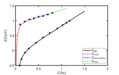
Figure 4: The potential of $\mathrm{QQq}$ and $\mathrm{Q\bar{Q}}$ at $T=0,\eta=0$. The solid black lines represent the $\mathrm{Q\bar{Q}}$ potential. The curves composed of dotted lines in three colors represent the $\mathrm{QQq}$ potential, with red indicating small $L$, blue for intermediate $L$, and green representing large $L$. The black solid dot represents the lattice data from quenched QCDKaczmarek et al. (2004); Yamamoto et al. (2008a); Najjar and Bali (2009).

Based on the model of heavy quarkonium in Refs. Kaczmarek et al. (2004); Kaczmarek and Zantow (2005); Kaczmarek (2007); Bazavov et al. (2018), similarly fitted to the Cornell potential for the $\mathrm{QQq}$, we can also determine the effective running coupling,

$$\alpha_{\mathrm{QQq}}=\frac{3L^{2}}{4}\frac{dE_{\mathrm{QQq}}}{dL},$$ (42)

to study the force between heavy quarks. It is the inter-two-quark potential in baryons which effectively includes the light-quark effects Yamamoto et al. (2008a). Moreover, it can be proven that the physical significance of Eq. (18) and Eq. (42) is the same, as both represent the effective coupling strength between heavy quarks. Thus, the effective running coupling of $\mathrm{QQq}$ is a function of the separation distance between the two heavy quarks as shown in Fig. 5. It can be seen that at small scales, $\mathrm{QQq}$ also exhibits asymptotic freedom behavior, and its range $(L<0.4\,\mathrm{fm})$ is broader compared to $\mathrm{Q\bar{Q}}$. Moreover, the effective running coupling of $\mathrm{QQq}$ is always smaller than that of $\mathrm{Q\bar{Q}}$ and is almost half of it. This is very close to the relationship between $A_{\mathrm{QQq}}$ and $A_{\mathrm{Q\bar{Q}}}$ fitted in the lattice Yamamoto et al. (2008a), which is due to the presence of the light quark reducing the interquark force Yamamoto et al. (2008b).

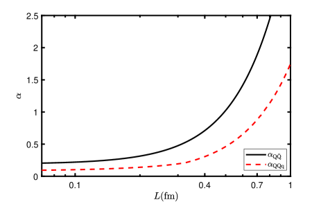
Figure 5: The effective running coupling of $\mathrm{QQq}$ and $\mathrm{Q\bar{Q}}$ at $T=0,\eta=0$. The red dashed line represents the $\mathrm{QQq}$, while the black solid line represents the $\mathrm{Q\bar{Q}}$.

III Numerical Results and Discussion

Before we proceed with the discussion, we need to establish the critical points (critical temperatures at different rapidities). At low temperatures and rapidities, $\mathrm{Q\bar{Q}}$ is confined, an imaginary wall $r_{w}$. The potential of the confined $\mathrm{Q\bar{Q}}$ increases with distance, but when it rises to a certain value, string breaking occurs, exciting light quark and anti-quark from the vacuum, with quarks always remaining confined within a hadron. At high temperatures and rapidities, $\mathrm{Q\bar{Q}}$ becomes deconfined, and the imaginary wall disappears. At this point, there is a maximum quark separation distance. When this distance is exceeded, the $\mathrm{Q\bar{Q}}$ no longer forms a U-shaped string configuration but instead consists of two straight string segments extending from the boundary to the horizon Finazzo and Noronha (2015). At this point, the potential also reaches its maximum, indicating that the $\mathrm{Q\bar{Q}}$ is screened at this point. This distance is known as the screening length. Considering string breaking or screening as a characteristic to distinguish between confinement and deconfinement, we can obtain the critical point of $\mathrm{Q\bar{Q}}$.

The critical points for $\mathrm{QQq}$ can be determined similarly, however, it possesses an additional property. At high temperature and/or rapidity QQq can dissociate at a certain distance. However, At extreme high temperature and/or rapidity the QQq can not exit judged from the force balance. Base on the previous discussion, we can draw out the state diagrams of $\mathrm{Q\bar{Q}}$ and $\mathrm{QQq}$ on the $(T,\eta)$ plane as in Fig. 6. The detailed discussions about the state diagram have already been completed in our previous work Liu et al. (2023).

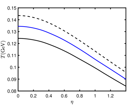
Figure 6: The black solid line is composed of the critical points of $\mathrm{QQq}$, the black dashed line is composed of the maximum $(T,\eta)$ points of $\mathrm{QQq}$; the blue solid line is composed of the critical points of $\mathrm{Q\bar{Q}}$.

III.1 Discussion about heavy quarkonium

Next, we discuss the temperature dependence of the effective running coupling of $\mathrm{Q\bar{Q}}$. From Fig. 6, it can be seen that critical temperature $T_{c}=0.1345\mathrm{GeV}$ when $\eta=0$. We calculate the effective running coupling in the range of $T/T_{c}\in[0,3]$ as shown in Fig. 7. When $T/T_{c}\in[0,1]$, $\mathrm{Q\bar{Q}}$ is in a confined state and the effect of temperature on the effective running coupling is relatively small. Therefore, our discussion of effective running coupling primarily concentrates on the deconfined state when $T/T_{c}>1$. Additionally, the string breaking can happen when $T/T_{c}<1$. The detailed discussion of string breaking at finite temperature and rapidity can be found in our previous works Liu et al. (2023).

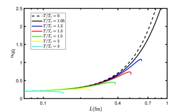
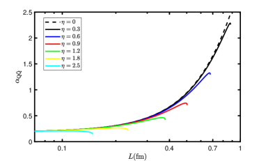
Figure 7: The left shows the temperature dependence of the effective running coupling for $\mathrm{Q\bar{Q}}$, where $\eta=0,T_{c}=0.1345\mathrm{GeV}$. The right shows the rapidity dependence of the effective running coupling for $\mathrm{Q\bar{Q}}$, at $T=0.1412\,\mathrm{GeV}$. These plots terminate at the screening distance.

From the left of Fig.7, it can be observed that the higher the temperature, the smaller the effective running coupling, and at small scales, the effective running coupling’s dependence on temperature is minor. This is understandable due to the asymptotic freedom of quarks at small scales. Additionally, the effect of temperature on effective running coupling primarily manifests in the maximum effective coupling constant $\tilde{\alpha}_{\mathrm{Q\bar{Q}}}(T,\eta)$, with the maximum effective coupling constant decreasing as the temperature increases, and the maximum coupling distance $L_{\tilde{\alpha}_{\mathrm{Q\bar{Q}}}}$ reduces. The impact of rapidity on the effective running coupling is similar to that of temperature, as shown in the right of Fig. 7. We choose a lower temperature, $T=0.1412\,\mathrm{GeV}$ (when $\eta=0,T=1.05T_{c}$), to observe a comprehensive process of the influence of rapidity on the effective running coupling. It can be seen that the greater the rapidity, the smaller the effective running coupling, and the smaller the maximum effective coupling constant. Furthermore, it is noteworthy that the screening distance $L_{screen}$ for $\mathrm{Q\bar{Q}}$ is greater than the maximum coupling distance $L_{\tilde{\alpha}_{\mathrm{Q\bar{Q}}}}$. Here we provide the definition: $\bigtriangleup L=L_{screen}-L_{\tilde{\alpha}_{\mathrm{Q\bar{Q}}}}$.

The maximum effective coupling constant as a function of $T/T_{c}$($\eta=0$) and $\eta/\eta_{c}$($T=0.1\mathrm{GeV}$) is shown in Fig. 8. From the left graph, it is apparent that when $T/T_{c}<1.5$, the maximum effective coupling constant rapidly decreases to a lower level as the temperature increases, and becomes relatively flat for $T/T_{c}>3$. The rapidity dependence of the maximum effective coupling constant is qualitatively similar to that of temperature; however, as a function of rapidity, it exhibits a more gradual decline and a broader range $(\eta/\eta_{c}<2)$ in the falling region. We present the screening distance and the maximum coupling distance in Fig. 9. The screening distance decreases with increasing temperature or rapidity, while the slope also decreases with increasing temperature or rapidity. The screening distance as a function of $T/T_{c}$ behaves similarly to that observed in the Ref. Kaczmarek and Zantow (2006). The $\bigtriangleup L$ increases with temperature and becomes conspicuously flat, and as a function of $\eta/\eta_{c}$, it displays a declining trend for $(\eta/\eta_{c}>3.5)$.

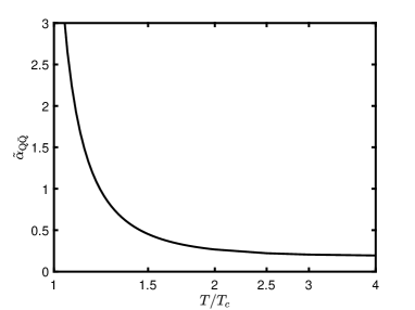
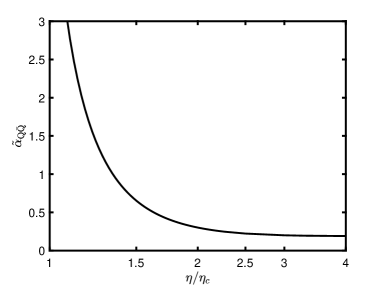
Figure 8: The left graph represents the maximum coupling $\tilde{\alpha}_{\mathrm{Q\bar{Q}}}$ as a function of $T/T_{c}$ at $\eta=0$. The right graph represents the maximum coupling as a function of $\eta/\eta_{c}$ at $T=0.1\mathrm{GeV}$.

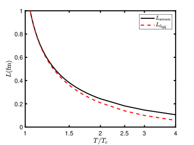
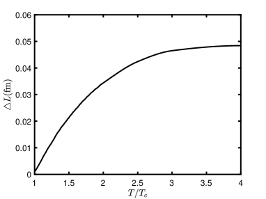
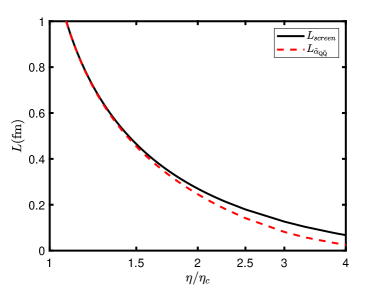
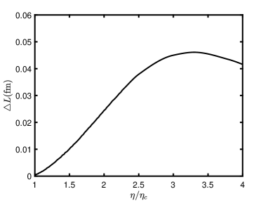
Figure 9: In the composite image, the left two images show the screening distance for $\mathrm{Q\bar{Q}}$ (solid black lines) and the maximum coupling distance (red dotted lines). The top image is plotted against $T/T_{c}$ at a fixed $\eta=0$, and the bottom image against $\eta/\eta_{c}$ at a fixed $T=0.1\mathrm{GeV}$. On the right, the two images illustrate the difference between these distances ($\bigtriangleup L$).

Next, we select three sets of data from the critical points in Fig. 6 for comparison: $(\eta,T_{c})=(0,0.1345)$, $(0.6,0.123)$, $(1.2,0.0985)$. From Fig. 10 and Fig. 11, it can be seen that although they both represent the function of the maximum effective coupling constant or screening distance with respect to $T/T_{c}$, there are slight differences under different rapidities. Specifically, the larger the rapidity, the smaller the maximum effective coupling constant and screening distance. This suggests that the larger the rapidity, the stronger the dependence of the maximum effective coupling constant and screening distance on temperature.

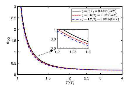
Figure 10: The maximum effective coupling constant $\tilde{\alpha}_{\mathrm{Q\bar{Q}}}$ as a function of $T/T_{c}$, where the solid black line represents $\eta=0$, the red dotted line represents $\eta=0.6$, and the blue dashed line represents $\eta=1.2$.

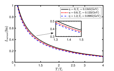
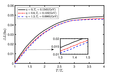
Figure 11: The left graph represents the screening distance as a function of $T/T_{c}$, and the right graph represents the $\bigtriangleup L$ as a function of $T/T_{c}$, where the solid black line represents $\eta=0$, the red dotted line represents $\eta=0.6$, and the blue dashed line represents $\eta=1.2$.

III.2 Discussion about doubly heavy baryon

As before, we first present the temperature dependence of the effective running coupling for $\mathrm{QQq}$ as shown in the left of Fig. 12, where $\eta=0,T_{c}=0.1245\,\mathrm{GeV}$. The rapidity dependence of the effective running coupling is shown in the right of Fig. 12, where $T=0.1245\,\mathrm{GeV}$. Their temperature and rapidity values reach up to the maximum values for which $\mathrm{QQq}$ can exist, $T\in[0,0.1435]\,(\eta=0)$, $\eta\in[0,0.751]\,(T=0.1245\,\mathrm{GeV})$. As shown in the two figures, the temperature and rapidity dependence of the effective running coupling for $\mathrm{QQq}$ is essentially consistent with that of $\mathrm{Q\bar{Q}}$. The higher the temperature and rapidity, the lower the effective running coupling curve. Furthermore, the distance at which $\mathrm{QQq}$ reaches maximum coupling is almost identical to the screening distance.

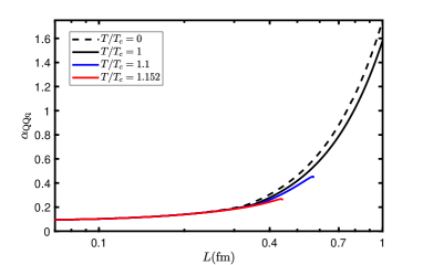
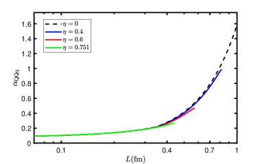
Figure 12: The left shows the temperature dependence of the effective running coupling for $\mathrm{QQq}$, where $\eta=0,T_{c}=0.1245\,\mathrm{GeV}$. At $T/T_{c}=1.152$, it reaches the maximum temperature for $\mathrm{QQq}$ with $\eta=0$. The right shows the rapidity dependence of the effective running coupling for $\mathrm{QQq}$, where $T=0.1245\,\mathrm{GeV}$. At $\eta=0.751$, it reaches the maximum rapidity for $\mathrm{QQq}$ with $T=0.1245\,\mathrm{GeV}$. These plots terminate at the screening distance.

We focus on the maximum effective coupling constant of $\mathrm{QQq}$, with the maximum effective coupling constant of $\mathrm{QQq}$ in relation to $\mathrm{Q\bar{Q}}$ displayed as the function of $T/T_{c}$ and $\eta/\eta_{c}$ in Fig. 13. And the screening distances for $\mathrm{QQq}$ and $\mathrm{Q\bar{Q}}$ is shown in Fig. 14. The graphs indicate that the maximum coupling constant of $\mathrm{QQq}$ quickly reduces with an increase in temperature or rapidity, and it consistently remains much lower than that of effective $\mathrm{Q\bar{Q}}$, showing a greater sensitivity to both temperature and rapidity. However, $\mathrm{QQq}$ is subject to a limit from the maximum $(T,\eta)$, and its graph ends as the maximum effective coupling constant begins to level off. Similarly, the screening distance for $\mathrm{QQq}$ is invariably shorter than that of $\mathrm{Q\bar{Q}}$, but it diminishes more quickly. Additionally, since $\mathrm{QQq}$ is always within the descending region, its trend of reduction with rapidity is consistently less intense than with temperature.

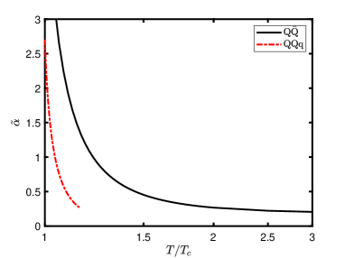
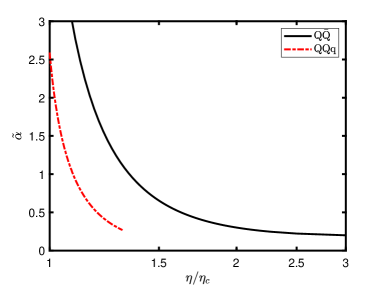
Figure 13: The left graph shows the maximum effective coupling constant $\tilde{\alpha}$ as a function of $T/T_{c}$ at $\eta=0$, where the $T_{c}=0.1245\mathrm{GeV}$ for $\mathrm{QQq}$ and $T_{c}=0.1345\mathrm{GeV}$ for $\mathrm{Q\bar{Q}}$. The right graph shows $\tilde{\alpha}$ as a function of $\eta/\eta_{c}$ at $T=0.1\mathrm{GeV}$, where the $\eta_{c}=1$ for $\mathrm{QQq}$ and $\eta_{c}=1.15$ for $\mathrm{Q\bar{Q}}$. The black solid line represents $\mathrm{Q\bar{Q}}$, and the red dotted line represents $\mathrm{QQq}$.

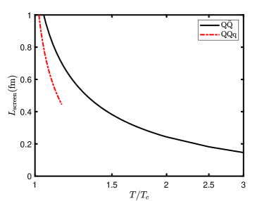
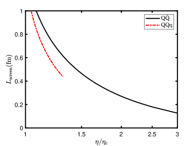
Figure 14: The left graph shows the screening distance as a function of $T/T_{c}$ at $\eta=0$, where the $T_{c}=0.1245\mathrm{GeV}$ for $\mathrm{QQq}$ and $T_{c}=0.1345\mathrm{GeV}$ for $\mathrm{Q\bar{Q}}$. The right graph shows the screening distance as a function of $\eta/\eta_{c}$ at $T=0.1\mathrm{GeV}$, where the $\eta_{c}=1$ for $\mathrm{QQq}$ and $\eta_{c}=1.15$ for $\mathrm{Q\bar{Q}}$. The black solid line represents $\mathrm{Q\bar{Q}}$, and the red dotted line represents $\mathrm{QQq}$.

IV Summary

In this work, we initially determined the parameters of our model by fitting the lattice potentials for $\mathrm{Q\bar{Q}}$ and $\mathrm{QQq}$. Subsequently, we calculated their the strength of the interaction which is defined as effective running coupling from the lattice. We discovered that, as a function of the distance between quarks, the effective coupling constant of $\mathrm{Q\bar{Q}}$ is always noticeably larger than that of $\mathrm{QQq}$, and the rate of increase with distance is more pronounced for $\mathrm{Q\bar{Q}}$ than for $\mathrm{QQq}$. Furthermore, the effective coupling constant for $\mathrm{Q\bar{Q}}$ is extremely low and flat within the range of $L<0.2\,\mathrm{fm}$, whereas for $\mathrm{QQq}$, this occurs approximately within $L<0.4\,\mathrm{fm}$. We interpret this as a manifestation of asymptotic freedom in the behavior of the effective coupling constants. Additionally, their effective coupling constants, as functions of distance, decrease with an increase in temperature or rapidity, which is particularly evident in the effective coupling constants at long distances, especially in the maximum effective coupling constant $\tilde{\alpha}$. The effective coupling constants for small scales remain almost unchanged with variations at finite temperature or rapidity.

Based on the holographic model, we have conducted a detailed analysis of the effective running coupling constant at finite temperature and rapidity in this paper. Through the above discussion, we can infer that the QQq system is less stable than the $\rm Q\bar{Q}$ system in the presence of temperature and rapidity. Furthermore, the study of the effective running coupling for the QQq system at finite magnetic fields and under rotation can also be conducted in the future work.

References

References

- Matsui and Satz (1986) T. Matsui and H. Satz, Phys. Lett. B 178, 416 (1986).
- Kharzeev and Satz (1995) D. Kharzeev and H. Satz, Quark-Gluon Plasma 2. Edited by HWA R C. Published by World Scientific Publishing Co. Pte. Ltd (1995).
- Witten (1998a) E. Witten, Adv. Theor. Math. Phys. 2, 505 (1998a), arXiv:hep-th/9803131 .
- Gyulassy and McLerran (2005) M. Gyulassy and L. McLerran, Nucl. Phys. A 750, 30 (2005), arXiv:nucl-th/0405013 .
- Jacobs and Wang (2005) P. Jacobs and X.-N. Wang, Prog. Part. Nucl. Phys. 54, 443 (2005), arXiv:hep-ph/0405125 .
- Carcamo Hernandez et al. (2014) A. E. Carcamo Hernandez, C. O. Dib, and A. R. Zerwekh, Eur. Phys. J. C 74, 2822 (2014), arXiv:1304.0286 [hep-ph] .
- Kaczmarek et al. (2004) O. Kaczmarek, F. Karsch, F. Zantow, and P. Petreczky, Phys. Rev. D 70, 074505 (2004), [Erratum: Phys.Rev.D 72, 059903 (2005)], arXiv:hep-lat/0406036 .
- Kaczmarek and Zantow (2005) O. Kaczmarek and F. Zantow, Phys. Rev. D 71, 114510 (2005), arXiv:hep-lat/0503017 .
- Kaczmarek (2007) O. Kaczmarek, PoS CPOD07, 043 (2007), arXiv:0710.0498 [hep-lat] .
- Bazavov et al. (2018) A. Bazavov, N. Brambilla, P. Petreczky, A. Vairo, and J. H. Weber (TUMQCD), Phys. Rev. D 98, 054511 (2018), arXiv:1804.10600 [hep-lat] .
- Laine (2006) M. Laine, PoS LAT2006, 014 (2006), arXiv:hep-lat/0612023 .
- Asaka et al. (2006) T. Asaka, M. Laine, and M. Shaposhnikov, JHEP 06, 053 (2006), arXiv:hep-ph/0605209 .
- Hindmarsh and Philipsen (2005) M. Hindmarsh and O. Philipsen, Phys. Rev. D 71, 087302 (2005), arXiv:hep-ph/0501232 .
- Rothkopf (2020) A. Rothkopf, Phys. Rept. 858, 1 (2020), arXiv:1912.02253 [hep-ph] .
- Aaij et al. (2017) R. Aaij et al. (LHCb), Phys. Rev. Lett. 119, 112001 (2017), arXiv:1707.01621 [hep-ex] .
- Aaij et al. (2018) R. Aaij et al. (LHCb), Phys. Rev. Lett. 121, 162002 (2018), arXiv:1807.01919 [hep-ex] .
- Giunti et al. (1991) C. Giunti, C. W. Kim, and U. W. Lee, Mod. Phys. Lett. A 6, 1745 (1991).
- Baikov et al. (2017) P. A. Baikov, K. G. Chetyrkin, and J. H. Kühn, Phys. Rev. Lett. 118, 082002 (2017), arXiv:1606.08659 [hep-ph] .
- Javidan et al. (2021) K. Javidan, M. M. Yazdanpanah, and H. Nematollahi, Eur. Phys. J. A 57, 78 (2021), arXiv:2003.06859 [hep-ph] .
- Aguilar et al. (2002) A. C. Aguilar, A. Mihara, and A. A. Natale, Phys. Rev. D 65, 054011 (2002), arXiv:hep-ph/0109223 .
- Lombardo and Mazzitelli (1997) F. C. Lombardo and F. D. Mazzitelli, Phys. Rev. D 55, 3889 (1997), arXiv:gr-qc/9609073 .
- Zhou et al. (2023) J. Zhou, S. Zhang, J. Chen, L. Zhang, and X. Chen, Phys. Lett. B 844, 138116 (2023), arXiv:2310.15609 [hep-ph] .
- Bloch et al. (2004) J. C. R. Bloch, A. Cucchieri, K. Langfeld, and T. Mendes, Nucl. Phys. B 687, 76 (2004), arXiv:hep-lat/0312036 .
- Deur et al. (2016) A. Deur, S. J. Brodsky, and G. F. de Teramond, Nucl. Phys. 90, 1 (2016), arXiv:1604.08082 [hep-ph] .
- Yu et al. (2022) Q. Yu, H. Zhou, X.-D. Huang, J.-M. Shen, and X.-G. Wu, Chin. Phys. Lett. 39, 071201 (2022), arXiv:2112.01200 [hep-ph] .
- Takaura et al. (2019) H. Takaura, T. Kaneko, Y. Kiyo, and Y. Sumino, JHEP 04, 155 (2019), arXiv:1808.01643 [hep-ph] .
- Chen et al. (2022a) X. Chen, L. Zhang, and D. Hou, Chin. Phys. C 46, 073101 (2022a), arXiv:2108.03840 [hep-ph] .
- Kaczmarek (2009) O. Kaczmarek, Eur. Phys. J. C 61, 811 (2009).
- Nijs et al. (2023) G. Nijs, B. Scheihing-Hitschfeld, and X. Yao (2023) arXiv:2312.12307 [hep-ph] .
- Shuryak (2017) E. Shuryak, Rev. Mod. Phys. 89, 035001 (2017), arXiv:1412.8393 [hep-ph] .
- Arnold et al. (2005) P. B. Arnold, J. Lenaghan, G. D. Moore, and L. G. Yaffe, Phys. Rev. Lett. 94, 072302 (2005), arXiv:nucl-th/0409068 .
- Yamamoto et al. (2008a) A. Yamamoto, H. Suganuma, and H. Iida, Phys. Rev. D 78, 014513 (2008a), arXiv:0806.3554 [hep-lat] .
- Najjar and Bali (2009) J. Najjar and G. Bali, PoS LAT2009, 089 (2009), arXiv:0910.2824 [hep-lat] .
- Maldacena (1998) J. M. Maldacena, Adv. Theor. Math. Phys. 2, 231 (1998), arXiv:hep-th/9711200 .
- Aharony et al. (2000) O. Aharony, S. S. Gubser, J. M. Maldacena, H. Ooguri, and Y. Oz, Phys. Rept. 323, 183 (2000), arXiv:hep-th/9905111 .
- Casalderrey-Solana et al. (2014) J. Casalderrey-Solana, H. Liu, D. Mateos, K. Rajagopal, and U. A. Wiedemann, Gauge/String Duality, Hot QCD and Heavy Ion Collisions (Cambridge University Press, 2014) arXiv:1101.0618 [hep-th] .
- Gubser (2013) S. S. Gubser, Found. Phys. 43, 140 (2013), arXiv:1103.3636 [hep-th] .
- Thakur et al. (2017) L. Thakur, N. Haque, and H. Mishra, Phys. Rev. D 95, 036014 (2017), arXiv:1611.04568 [hep-ph] .
- Escobedo et al. (2013) M. A. Escobedo, F. Giannuzzi, M. Mannarelli, and J. Soto, Phys. Rev. D 87, 114005 (2013), arXiv:1304.4087 [hep-ph] .
- Song et al. (2008) T. Song, Y. Park, S. H. Lee, and C.-Y. Wong, Phys. Lett. B 659, 621 (2008), arXiv:0709.0794 [hep-ph] .
- Benzahra (2004) S. C. Benzahra, Afr. J. Math. Phys. 1, 191 (2004), arXiv:hep-ph/0204177 .
- Liu et al. (2007) H. Liu, K. Rajagopal, and U. A. Wiedemann, Phys. Rev. Lett. 98, 182301 (2007), arXiv:hep-ph/0607062 .
- Chen et al. (2021) X. Chen, L. Zhang, D. Li, D. Hou, and M. Huang, JHEP 07, 132 (2021), arXiv:2010.14478 [hep-ph] .
- Chen et al. (2018) X. Chen, S.-Q. Feng, Y.-F. Shi, and Y. Zhong, Phys. Rev. D 97, 066015 (2018), arXiv:1710.00465 [hep-ph] .
- Finazzo and Noronha (2015) S. I. Finazzo and J. Noronha, JHEP 01, 051 (2015), arXiv:1406.2683 [hep-th] .
- Ali-Akbari et al. (2014) M. Ali-Akbari, D. Giataganas, and Z. Rezaei, Phys. Rev. D 90, 086001 (2014), arXiv:1406.1994 [hep-th] .
- Andreev (2022a) O. Andreev, Nucl. Phys. B 977, 115724 (2022a), arXiv:2106.14716 [hep-ph] .
- Krishnan (2008) C. Krishnan, JHEP 12, 019 (2008), arXiv:0809.5143 [hep-th] .
- Chernicoff et al. (2013) M. Chernicoff, D. Fernandez, D. Mateos, and D. Trancanelli, JHEP 01, 170 (2013), arXiv:1208.2672 [hep-th] .
- Bitaghsir Fadafan and Tabatabaei (2016) K. Bitaghsir Fadafan and S. K. Tabatabaei, J. Phys. G 43, 095001 (2016), arXiv:1501.00439 [hep-th] .
- Zhou et al. (2020) J. Zhou, X. Chen, Y.-Q. Zhao, and J. Ping, Phys. Rev. D 102, 086020 (2020), arXiv:2006.09062 [hep-ph] .
- Feng et al. (2020) S.-Q. Feng, Y.-Q. Zhao, and X. Chen, Phys. Rev. D 101, 026023 (2020), arXiv:1910.05668 [hep-ph] .
- Zhou et al. (2021) J. Zhou, X. Chen, Y.-Q. Zhao, and J. Ping, Phys. Rev. D 102, 126029 (2021).
- Alexandrou et al. (2002) C. Alexandrou, P. De Forcrand, and A. Tsapalis, Nucl. Phys. B Proc. Suppl. 106, 403 (2002), arXiv:hep-lat/0110115 .
- Alexandrou et al. (2003) C. Alexandrou, P. de Forcrand, and O. Jahn, Nucl. Phys. B Proc. Suppl. 119, 667 (2003), arXiv:hep-lat/0209062 .
- Takahashi et al. (2002) T. T. Takahashi, H. Suganuma, Y. Nemoto, and H. Matsufuru, Phys. Rev. D 65, 114509 (2002), arXiv:hep-lat/0204011 .
- Andreev (2021a) O. Andreev, JHEP 05, 173 (2021a), arXiv:2007.15466 [hep-ph] .
- Andreev (2016a) O. Andreev, Phys. Lett. B 756, 6 (2016a), arXiv:1505.01067 [hep-ph] .
- Andreev (2016b) O. Andreev, Phys. Rev. D 93, 105014 (2016b), arXiv:1511.03484 [hep-ph] .
- Andreev (2020a) O. Andreev, Phys. Lett. B 804, 135406 (2020a), arXiv:1909.12771 [hep-ph] .
- Andreev (2021b) O. Andreev, Phys. Rev. D 104, 026005 (2021b), arXiv:2101.03858 [hep-ph] .
- Andreev (2023a) O. Andreev, Phys. Rev. D 107, 026023 (2023a), arXiv:2211.12305 [hep-ph] .
- Andreev (2022b) O. Andreev, Phys. Rev. D 106, 066002 (2022b), arXiv:2205.12119 [hep-ph] .
- Andreev (2023b) O. Andreev, Phys. Rev. D 108, 106012 (2023b), arXiv:2306.08581 [hep-ph] .
- Mei et al. (2023) J. Mei, T. Xia, and S. Mao, Phys. Rev. D 107, 074018 (2023), arXiv:2212.04778 [hep-ph] .
- Andreev (2022c) O. Andreev, Phys. Rev. D 105, 086025 (2022c), arXiv:2111.14418 [hep-ph] .
- Mei et al. (2024) J. Mei, R. Wen, S. Mao, M. Huang, and K. Xu, (2024), arXiv:2402.19193 [hep-ph] .
- Andreev and Zakharov (2007) O. Andreev and V. I. Zakharov, JHEP 04, 100 (2007), arXiv:hep-ph/0611304 .
- Andreev (2008) O. Andreev, Phys. Lett. B 659, 416 (2008), arXiv:0709.4395 [hep-ph] .
- Andreev (2024) O. Andreev, Phys. Rev. D 109, 106001 (2024), arXiv:2402.09026 [hep-ph] .
- Chen et al. (2022b) X. Chen, B. Yu, P.-C. Chu, and X.-h. Li, Chin. Phys. C 46, 073102 (2022b), arXiv:2112.06234 [hep-ph] .
- Wen et al. (2024) N. Wen, X. Cao, J. Chao, and H. Liu, Phys. Rev. D 109, 086021 (2024), arXiv:2402.06239 [hep-th] .
- Liang et al. (2023) W. Liang, X. Cao, H. Liu, and D. Li, Phys. Rev. D 108, 096019 (2023), arXiv:2307.03708 [hep-ph] .
- Cao et al. (2022) X. Cao, M. Baggioli, H. Liu, and D. Li, JHEP 12, 113 (2022), arXiv:2210.09088 [hep-ph] .
- Cao et al. (2023) X. Cao, J. Chao, H. Liu, and D. Li, Phys. Rev. D 107, 086001 (2023), arXiv:2204.11604 [hep-ph] .
- Yang and Yuan (2015) Y. Yang and P.-H. Yuan, JHEP 12, 161 (2015), arXiv:1506.05930 [hep-th] .
- Colangelo et al. (2011) P. Colangelo, F. Giannuzzi, and S. Nicotri, Phys. Rev. D 83, 035015 (2011), arXiv:1008.3116 [hep-ph] .
- Andreev (2018a) O. Andreev, Phys. Rev. D 98, 066007 (2018a), arXiv:1804.09529 [hep-ph] .
- Andreev (2018b) O. Andreev, Mod. Phys. Lett. A 33, 1850041 (2018b), arXiv:1707.05045 [hep-ph] .
- Witten (1998b) E. Witten, JHEP 02, 006 (1998b), arXiv:hep-th/9712028 .
- Gukov et al. (1998) S. Gukov, M. Rangamani, and E. Witten, JHEP 12, 025 (1998), arXiv:hep-th/9811048 .
- Andreev (2020b) O. Andreev, Phys. Rev. D 101, 106003 (2020b), arXiv:2003.09880 [hep-ph] .
- Erlich et al. (2005) J. Erlich, E. Katz, D. T. Son, and M. A. Stephanov, Phys. Rev. Lett. 95, 261602 (2005), arXiv:hep-ph/0501128 .
- Yamamoto et al. (2008b) A. Yamamoto, H. Suganuma, and H. Iida, Prog. Theor. Phys. Suppl. 174, 270 (2008b), arXiv:0805.4735 [hep-ph] .
- Liu et al. (2023) X. Liu, J.-J. Jiang, X. Chen, M. Fujita, and A. Watanabe, (2023), arXiv:2310.08146 [hep-ph] .
- Kaczmarek and Zantow (2006) O. Kaczmarek and F. Zantow, PoS LAT2005, 177 (2006), arXiv:hep-lat/0510093 .