Slope of Magnetic Field-Density Relation as An Indicator of Magnetic Dominance

Abstract

The electromagnetic field is a fundamental force in nature that regulates the formation of stars in the universe. Despite decades of efforts, a reliable assessment of the importance of the magnetic fields in star formation relations remains missing. In star-formation research, our acknowledgment of the importance of magnetic field is best summarized by the Crutcher et al. 2010 $B$-$\rho$ relation

$${\rm log}B(\rho)/G=\left\{\begin{aligned} -5,\,\,{\rm if}\,\rho\,\lesssim\,10^{-20}\,{\rm g\,cm}^{-3}\\ \frac{2}{3}\cdot{\rm log}\rho+{\rm log}\rho_{0},\,\,{\rm if}\,\rho\,\gtrsim\,10^{-20}\,{\rm g\,cm}^{-3}\end{aligned}\right.$$

whose interpretation remains controversial (Zhang et al., 2019; Li, 2021; Cao & Li, 2023). The relation is either interpreted as proof of the importance of a magnetic field in the collapse Zhang et al. (2019), or the result of self-similar collapse where the role of the magnetic is secondary to gravity Li & Burkert (2018). Using simulations, we find a fundamental relation, ${\cal M}_{\rm A}$-k_B-ρ(slope of $B-\rho$ relation) relation:

$$\rm\frac{{\cal M}_{\rm A}}{{\cal M}_{\rm A,c}}=k_{B-\rho}^{\cal K}\approx\frac{{\cal M}_{\rm A}}{7.5}\approx k_{B-\rho}^{1.7\pm 0.15}.$$

This fundamental B-$\rho$-slope relation enables one to measure the Alfvénic Mach number, a direct indicator of the importance of the magnetic field, using the distribution of data in the B-$\rho$ plane. It allows us to drive the following empirical $B-\rho$ relation

$$\frac{B}{B_{c}}={\rm exp}\left(\left(\frac{\gamma}{{\cal K}}\right)^{-1}\left(\frac{\rho}{\rho_{c}}\right)^{\frac{\gamma}{{\cal K}}}\right)\approx\frac{B}{10^{-6.3}{\rm G}}\approx{\rm exp}\left(9\left(\frac{\rho}{10^{-16.1}{\rm g\,cm^{-3}}}\right)^{0.11}\right)\;,$$

which offers an excellent fit to the Cruther et al. data, where we assume ${\cal M}_{\rm A}-\rho$ relation ($\frac{{\cal M}_{\rm A}}{{\cal M}_{\rm A,c}}=\left(\frac{\rho}{\rho_{c}}\right)^{\gamma}\approx{\cal M}_{\rm A}/{7.5}\approx\left(\rho/{10^{-16.1}{\rm g\,cm^{-3}}}\right)^{\rm 0.19}$).

The foundational ${\cal M}_{\rm A}-{\rm k}_{B-\rho}$ relation provides an independent way to measure the importance of magnetic field against the kinematic motion using multiple magnetic field measurements. Our approach offers a new interpretation of the (Crutcher et al., 2010), where a gradual decrease in the importance of B at higher densities is implied.

1 Background

The magnetic field is a fundamental force that plays a crucial role in the evolution of interstellar gas and star formation (Collins et al., 2012; Li, 2021; Pattle et al., 2023) through magnetic force and it also changes the initial condition (Yang et al., 2023) by affecting the transport of cosmic rays.

Despite decades of research, constraints on the importance of magnetic fields remain sparse. There are two approaches. The first one involves the measurement of dimension numbers which reflects the importance of the magnetic fields. One example is the mass-to-flux ratio, which is the ratio between mass and magnetic flux (Nakano, 1978; Crutcher et al., 2004). The second approach is to derive scaling relations between the magnetic field and density(Crutcher et al., 2010; Zhang et al., 2019; Cao & Li, 2023), which serve as bridges between theory and observations.

The empirical magnetic field density relation ($B-\rho$ relation) is an empirical relation describing the magnetic field strength in the interstellar constructed using a sample of regions with Zeeman observations (Crutcher et al., 2010; Zhang et al., 2019; Jiang et al., 2020; Cao & Li, 2023). The relation can be described using different functions, such as

$${\rm log}B(\rho)/G=\left\{\begin{aligned} -5,\,\,{\rm if}\,\rho\,\lesssim\,10^{-20}\,{\rm g\,cm}^{-3}\\ \frac{2}{3}\cdot{\rm log}\rho+{\rm log}\rho_{0},\,\,{\rm if}\,\rho\,\gtrsim\,10^{-20}\,{\rm g\,cm}^{-3}\end{aligned}\right.$$ (1)

The classical $B-\rho$ relation is an empirical relation, which does not explain how the B-field evolves with density growing. Zhang et al. 2019; Cao & Li 2023 explain a part of classical $B-\rho$ relation with the $\frac{2}{3}$ power-law exponent being caused by the collapse of star formation This exponent of $B-\rho$ in star-forming can be linked to the density profile of the region, where $B\propto\rho^{1/2}$ is related to the density profile of $\rho\sim r^{-2}$ (Li & Burkert, 2018). The $B-\rho$ relation is affected transiently by galactic magnetic field morphology (Konstantinou et al., 2024).

The magnetic field-density relation, although widely cited, is non-trivial to interpret because both the magnetic field and gravitational force are long-range forces where the scale information is critical (Li & Burkert, 2018). For example, the energy balance of a cloud reads $B^{2}r^{3}\,\approx\rho^{2}r^{5}$, where the scale information is an essential part. To address the energy balance, one should perform joint analyses of the magnetic field-density relation and density-scale relation (Li & Burkert, 2018).

$B-\rho$ relation derived from several observations targeting single regions can provide crucial insight into the importance of B field (Crutcher et al., 2010; Li et al., 2015; Kandori et al., 2018; Jiang et al., 2020; Wang et al., 2020). When targeting individual regions, one eliminates the uncertainties in the scale. $B-\rho$ relation constructed in this way can better reflect the interplay between turbulence, gravity, and the B-field.

The scope of this paper is to offer a direct interpretation of the slope of the $B-\rho$ relation, as a direct indicator of the importance of magnetic field. Compared to the mass-to-flux ratio, which is indirect diagnostic and can be hard to measure, the Alfenvi Mach number is a direct indicator of the importance and is directly measurable using the slope. Our approach also allows for re-interpreting the (Crutcher et al., 2010). Using numerical simulation, we establish a fundamental link between the slope, $d({\rm log}B)/d({\rm log}\rho)$ with the importance of magnetic field measured in terms of the Alfvén Mach number ${\cal M}_{\rm A}$. This allows us to evaluate the importance of the magnetic field directly from observations even to approach the fundamental $B-\rho$ relation.

2 Alfvénic Mach Number & Fundamental $B-\rho$ Relation

2.1 Slope of $B-\rho$ Relation: An Indicator of ${\cal M}_{\rm A}$

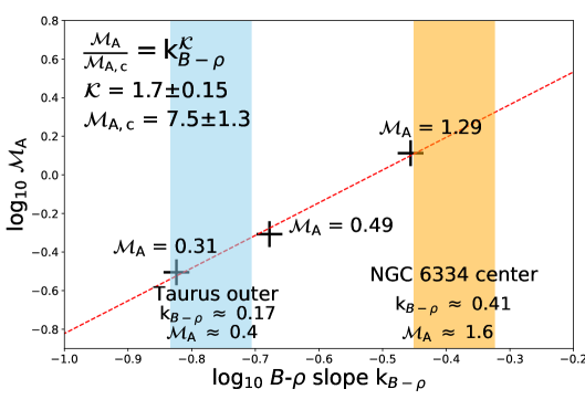
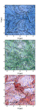
Figure 1: The B-$\rho$ slope k_B-ρ and Alfvén Mach number ${\cal M}_{\rm A}$ relation. The crosses in the left pane; show the position of three re-scaled simulations with $\beta$ as 0.2, 2, and 20, in k_B-ρ and ${\cal M}_{\rm A}$ plane, which the k_B-ρ is the B-$\rho$ slope of the mean density in various simulations. The red dash line shows fitted B-$\rho$ slope k_B-ρ and Alfvén Mach number ${\cal M}_{\rm A}$ relation. The blue and orange columns show the k_B-ρ position of the previous observation, Taurus and NGC 6334 center region, respectively. The right panels depict the spatial distribution of the magnetic field (B-field) in a two-dimensional x-y slice, which comes from simulations with different $\beta$ and Alfvén Mach number ${\cal M}_{\rm A}$. The color-coded maps represent these simulations as follows: the blue map corresponds to $\beta=0.2$ and Alfvén Mach number ${\cal M}_{\rm A}$ = 0.31, the green map to $\beta=2$ with ${\cal M}_{\rm A}$ = 0.49, and the red map to $\beta$ = 20 with ${\cal M}_{\rm A}$ = 2.36. The vector arrows illustrate the local magnetic field orientations. The background contours illustrate the density distribution, ranging from 10^-21 to 10^-18 g cm^-3.

To establish ration between $B-\rho$ and ${\cal M}_{\rm A}$, we select a numerical magnetohydrodynamic (MHD) simulation (Collins et al., 2012; Burkhart et al., 2015). The initial conditions are generated by a PPML code without self-gravity (Ustyugov et al., 2009), after which the main simulation was performed using AMR code Enzo(Bryan et al., 1995; O’Shea et al., 2004) where self-gravity is included. In both simulations, the equation of state is isothermal.

The relatively short simulation time ($0.8\,\rm Myr$) means the effect of self-gravity is only noticeable in the regions of the highest density . The observed $B-\rho$ relation mostly reflects the interplay between the magnetic field and turbulence cascade, which is the main focus of this work.

We choose three simulations of different initial degrees of magnetization $\beta_{0}$ = ${8\pi c_{s}^{2}\rho_{0}}/{B_{0}^{2}}$ = 0.2, 2, 20. The slopes of the $B-\rho$ relation can be derived after some averages (Method A). The Alfvén Mach number ${\cal M}_{\rm A}$ in various simulations can be calculated by the total energy ratio between the magnetic energy $E_{B}$ and kinetic energy $E_{k}$:

$${\cal M}_{\rm A}=\frac{\sqrt{4\pi\rho}\sigma_{v}}{B}=\frac{0.5\rho\sigma_{v}^{2}}{B^{2}/8\pi}=\frac{\sum e_{\rm k}}{\sum e_{B}},$$ (2)

where the ${\cal M}_{\rm A}$ in strong, medium, and weak magnetic field states can be estimated as 0.31, 0.49, and 1.29, respectively. The Alfvénic Mach numbers ${\cal M}_{\rm A}$ are measured at the time of the snapshots (Method A), which is different from the Alfvénic Mach numbers inferred from the initial conditions, due to the dissipation of turbulence and the amplification of the magnetic field.

We then plot the Mach number against the measured slope of the $B-\rho$ (see Fig. 4), to reveal a surprisingly simple relation between the slope of the $B-\rho$ relation (k_B-ρ = d (log₁₀ $B$) / d (log₁₀ $\rho$)) and the Alfvén Mach number ${\cal M}_{\rm A}$,

$$\rm\frac{{\cal M}_{\rm A}}{{\cal M}_{\rm A,c}}=k_{B-\rho}^{\cal K},$$ (3)

where the ${\cal K}$ = 1.7$\pm$0.15, and the ${\cal M}_{\rm A,c}$ is the characteristic ${\cal M}_{\rm A}$ ($\sim$ 7.5$\pm$1.3, see Fig. 1). The degree of magnetization quantified using ${\cal M}_{\rm A}$ determines the power-law exponent between density and magnetic field. The ${\cal M}_{\rm A}-{\rm k}_{B-\rho}$ relation could be a fundamental relation in natural. An intuitive explanation for the correlation between the stronger magnetic field and shallower magnetic field-density relation is that a strong field can regulate the way collapse occurs, such that the matter accumulates along the field lines, weakening the correlation between B and $\rho$.

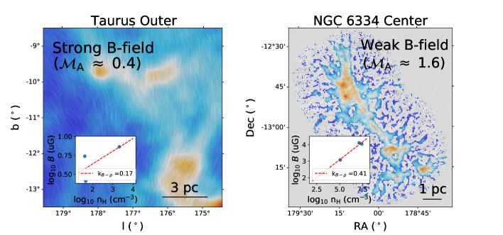
Figure 2: B-field and slope of $B-\rho$ relation in Taurus outer and NGC 6334 center regions. The panels show the magnetic field morphology and slope of $B-\rho$ relation in Tauras outer region and NGC 6334 center region. The $B-\rho$ distribution is derived from Zeeman observations in Tauras outer region (Crutcher et al., 2010; Ching et al., 2022) and that of NGC 6334 from Li et al. 2015. The magnetic field morphology is derived by Planck 353 GHz dust polarization (Planck Collaboration et al., 2020) and JCMT 850 $\mu$m dust polarization (Arzoumanian et al., 2021).

2.2 Determining the Importance of B-field using the ${\cal M}_{\rm A}$- k_B-ρ relation

${\cal M}_{\rm A}$ is a fundamental physical quantity that directly characterizes the importance of the magnetic field. The fact that this quantity is directly related to the slope of the $B-\rho$ relation provides a new way to study the importance of the magnetic field (see Sect. 2.1). However, to construct this single-region $B-\rho$ relations, we require multi-scales, multi-densities observations towards single regions (Methods D). Another case is the outer region of the Taurus molecular cloud, where multiple constraints of the magnetic field strength using Zeeman splitting Crutcher et al. (2010); Ching et al. (2022) are available.

We reveal vastly different roles of the magnetic field (see Fig. 2) by applying our results to both clouds. Toward the Taurus outer region, using Zeeman observations (Crutcher et al., 2010; Ching et al., 2022), we estimate a ${\cal M}_{\rm A}$ of 0.8, indicative of a relatively strong (dynamically significant) magnetic field. Towards the NGC 6334 center region, the ${\cal M}_{\rm A}$ is estimated as 3.0, implying a weak (dynamically weak) magnetic field.

Our assessment of the importance of the magnetic field is consistent with the behavior of these regions as reported in the literature (Ching et al., 2022; Li et al., 2015): The strong magnetic field observed towards the outer region of the Taurus molecular cloud, where ${\cal M}_{\rm A}$ ($\sim$ 0.4) indicates that the B-field is strong enough to dominate the gas evolution. This is consistent with conclusions from previous studies Heyer et al. (2016); Tritsis & Tassis (2016). At the Taurus outer region, people have observed striations which are taken as signs of the dominance MHD wave (Heyer et al., 2016; Tritsis & Tassis, 2016) – a phenomenon that occurs only if the B-field is strong enough. Towards the dense part where our observations target, it is found that denser gas has lost a significant amount of magnetic flux as compared to the diffuse envelope (Ching et al., 2022), and this critical transition, and agrees well with our estimate where $\sqrt{E_{B}/E_{k}}\propto{\cal M}_{\rm A}$. Towards the central region NGC 6334, we find that kinetic energy is far above the magnetic energy (${\cal M}_{\rm A}\approx$1.6), dynamically insignificant magnetic field). This is consistent with NGC 6334 being one the most active star-forming regions with a high fraction of dense gas Schneider et al. (2022).

Using the fundamental ${\cal M}_{\rm A}-{\rm k}_{B-\rho}$ relation (Eq. 3), we can use the slope of $B-\rho$ relation to estimate the Alfvén Mach number ${\cal M}_{\rm A}$, which determine the importance of B-field.

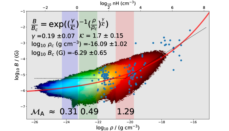
Figure 3: $B-\rho$ relation in multi-regions. This panel displays the relation between magnetic field (B) and density ($\rho$) following the exponential function. The red line presents the exponential $B-\rho$ relation derived by ${\cal M}_{\rm A}$-k_B-ρ relation and ${\cal M}_{\rm A}-\rho$ relation. Within this panel, the blue scatter points represent the distribution of sources measured with the Zeeman effect in the B-$\rho$ space, as detailed in (Crutcher et al., 2010). The black dashed line shows the old version (power law) $B-\rho$ relation fitted by the Zeeman source (blue scatters). The blue, green, and red clouds display the distribution of rescaling simulations with various ${\cal M}_{\rm A}$ as 0.31, 0.49, and 1.29, respectively. The blue, green, and red columns show the ${\cal M}_{\rm A}$ and mean density of rescaling simulations with various ${\cal M}_{\rm A}$ as 0.31, 0.49, and 1.29, respectively.

2.3 Fundamental $B-\rho$ relation

In the past, a convenient way to study magnetic field was to plot the field strength against the gas density, forming the magnetic field-density relation (Crutcher et al., 2010; Zhang et al., 2019; Cao & Li, 2023). This multi-region magnetic field-density relation is constructed from observations of different regions which have different sizes and geometries. The plural nature of this multi-region magnetic field-density relation makes it not particularly useful in estimating the ${\cal M}_{\rm A}$. However, we can decipher this relation using a minimum of assumptions.

We start from the fundamental ${\cal M}_{\rm A}-{\rm k}_{B-\rho}$ relation (Eq. 3), and assume another relation between Alfvén Mach number ${\cal M}_{\rm A}$ and density $\rho$ as a power low:

$$\frac{{\cal M}_{\rm A}}{{\cal M}_{\rm A,c}}=\left(\frac{\rho}{\rho_{c}}\right)^{\gamma}\;,$$ (4)

The fundamental $B-\rho$ relation can be derived by combining fundamental ${\cal M}_{\rm A}$-k_B-ρ relation (Eq. 3) with the empirical ${\cal M}_{\rm A}$-$\rho$ relation (Eq.4) :

$$\large\frac{B}{B_{c}}={\rm exp}\left(\left(\frac{\gamma}{{\cal K}}\right)^{-1}\left(\frac{\rho}{\rho_{c}}\right)^{\frac{\gamma}{{\cal K}}}\right)\;,$$ (5)

and by fitting Eq.5 to the observational data from Crutcher et al. (2010), assuming ${\cal K}$ =1.7$\pm$0.15 (Sec.2.1), we find $\gamma=0.19\pm 0.07$, ${\rm log_{10}}\rho_{\rm c}/{\rm(g\,cm^{-3})}=16.09\pm 1.02$, and ${\rm log_{10}}B_{\rm c}/{\rm(G)}=-6.29\pm 0.65$. This relation (Eq. 5) perfectly crosses all Zeeman observations and three MHD simulations and agrees to the classical $B-\rho$ relation (Crutcher et al., 2010; Zhang et al., 2019; Jiang et al., 2020) In the diffuse region, the B-field slowly grows with density increasing. In high density region ($\rho\,\sim\,10^{-18}$ g cm^-3), the slope of $B-\rho$ relation is also up to 2/3, which is caused by star formation (Zhang et al., 2019; Li, 2021).

Our fitting implies

$$\frac{{\cal M}_{\rm A}}{{\cal M}_{\rm A,c}}=(\frac{\rho}{\rho_{c}})^{0.19\pm 0.07}\;,$$ (6)

which is a general relation connecting the degrees of magnetization of clouds in the Milky Way with the density. At low density (10^-22 g cm^-3), the magnetic field is non-negligible. As the density increases, the importance of the magnetic field is gradually diminished. The high-density regions are mostly kinematically-dominated. This flat ${\cal M}_{\rm A}-\rho$ relation (${\cal M}_{\rm A}\,\propto$ $\rho^{0.19\pm 0.07}$) also agrees to actual observations (see the Fig.2 of Pattle et al. 2023).

This gradual decrease in the importance of the magnetic field is consistent with observational data. At the low-density end, the outer region of Taurus (Heyer et al., 2016; Tritsis & Tassis, 2016) and Musca (Tritsis & Tassis, 2018) molecular clouds have striations (MHD wave, the feature of strong magnetic field state), indicative of strong, dynamically-important magnetic field. At intermediate densities, the increase of the gas density can be accompanied by an increase of the mass-to-flux ratio, and a gradual decrease of the importance of the magnetic field, as observed in the L1544 region (Ching et al., 2022), and most high-density regions appears to be kinematically-dominated, such as NGC 6334 (Li et al., 2015), Ser-emb 8 (Matthews et al., 2009; Hull et al., 2014), and W51 (Koch et al., 2018).

3 Conclusion

We find that the slope of the magnetic field-density relation k_B-ρ = ${\rm d(log_{10}B)}/{\rm d(log_{10}\rho)}$ linked to the Alfvén Mach number, ${\cal M}_{\rm A}$ using numerical simulation results,

$$\rm\frac{{\cal M}_{\rm A}}{{\cal M}_{\rm A,c}}=k_{B-\rho}^{\cal K}\approx\frac{{\cal M}_{\rm A}}{11.0}\approx k_{B-\rho}^{\rm 1.7\pm 0.15},$$

where the ${\cal K}$ = 1.7$\pm$0.15, and the ${\cal M}_{\rm A,c}$ is the characteristic ${\cal M}_{\rm A}$ ($\sim$ 7.5$\pm$1.3). This fundamental relation results from the interplay between turbulence cascade and the implication of magnetic field in MHD turbulence. This fundamental relation allows us to estimate Ma using the slope of the B-rho relation. We apply this technique to several regions and find that the estimated ${\cal M}_{\rm A}$ values exhibit clear correlations between ${\cal M}_{\rm A}$ with the observed star formation activities.

We find that the empirical $B-\rho$ relation can be explained using our fundamental relation, together with a relation between Ma and gas density. The ${\cal M}_{\rm A}-\rho$ relation reads

$$\rm\frac{{\cal M}_{\rm A}}{{\cal M}_{\rm A,c}}=\left(\frac{\rho}{\rho_{c}}\right)^{\gamma}\approx\frac{{\cal M}_{\rm A}}{7.5}\approx\left(\frac{\rho}{10^{-16.1}{\rm g\,cm^{-3}}}\right)^{\rm 0.19\pm 0.07}\;,$$

and the $B-\rho$ relation takes the following form

$$\frac{B}{B_{c}}={\rm exp}\left(\left(\frac{\gamma}{{\cal K}}\right)^{-1}\left(\frac{\rho}{\rho_{c}}\right)^{\frac{\gamma}{{\cal K}}}\right)\approx\frac{B}{10^{-6.3}{\rm G}}\approx{\rm exp}\left(9\left(\frac{\rho}{10^{-16.1}{\rm g\,cm^{-3}}}\right)^{0.11}\right)\;,$$

which provides a good fit to existing observational data. This fitting result reveals a general trend where a general decrease in the importance of the magnetic field accompanies the increase in the gas density.

The fundamental ${\cal M}_{\rm A}-{\rm k}_{B-\rho}$ relation provides an independent way to estimate the importance of the magnetic field, and it can be widely applied to further observations. The decreasing importance of magnetic field at higher density appears consistent with most of the existing observations and will be tested against future results.

Method

Appendix A Simulation

The numerical simulation of molecular cloud selected in this work is identified within the three $\beta_{0}$ simulations applied by the constrained transport MHD option in Enzo (MHDCT) code (Collins et al., 2010; Burkhart et al., 2015). The simulation conducted in this study analyzed the impact of self-gravity and magnetic fields on supersonic turbulence in isothermal molecular clouds, using high-resolution simulations and adaptive mesh refinement techniques. which detail in shown in (Collins et al., 2012; Burkhart et al., 2015, 2020). The Enzo simulation with three dimensionless parameters provides us with massive information on physical processes:

$${\cal M}_{s}=\frac{v_{\rm rms}}{c_{s}}=9$$ (A1)

$$\alpha_{vir}=\frac{5v_{\rm rms}^{2}}{3G\rho_{0}L_{0}^{2}}=1$$ (A2)

$$\beta_{0}=\frac{8\pi c_{s}^{2}\rho_{0}}{B_{0}^{2}}=0.2,2,20$$ (A3)

where v_rms is the rms velocity fluctuation, c_s is sonic speed, $\rho_{0}$ is mean density, and $B_{0}$ is the mean magnetic field strength. With the same sonic Mach number ${\cal M}_{\rm s}$ and viral parameter $\alpha_{vir}$ in initial conditions, the difference only exists in initial magnetic pressure $\beta-0$ with various B-field strength, The $\beta_{0}$ as 0.2, 2, and 20 present the strong B-field state, medium B-field, and weak B-field state. The clouds are in three different evolutionary stages started with self-gravity existing at 0.6$t_{\rm ff}$($\sim$ 0.76 Myr), where $t_{\rm ff}$ represents 1.1$((n_{H}/10^{3})^{-1/2}$ Myr (Collins et al., 2012; Burkhart et al., 2015). Due to the short timescale of evolution, the gravitational collapse could barely affect the B-$\rho$ relation in the simulation The size of these molecular clouds is around 4.6³ pc (256³ pixels), with one-pixel size of approximately 0.018 pc (Burkhart et al., 2015). Fig. 3 show the distribution of B-field and density with three $\beta$ in the timescale of 0.6 $t_{\rm ff}$ ($\sim$ 0.76 Myr).

In this Enzo simulation, the thermal energy is located at the low state (${\cal M}_{s}$ = 9). Their timescale of evolution stage is 0.6 $t_{\rm ff}$, around 0.76 Myr, which the timescale starts from when interstellar media collapse. Due to the short evolutionary time ($\sim$ 3.85 $\times$ 10^-21 g cm^-3, or 821 cm^-3), the gravitational energy less affects the system in simulation. With the similar mean density $\rho_{0}$ in these simulations, the different $\beta_{0}$ ($\sim$0.2, 2, 20) present the different magnetic field states, strong B-field, stronger B-field (weaker than strong B-field but stronger than weak B-field), and weak B-field. The energy ratio between kinetic energy $E_{\rm k}$ and magnetic energy $E_{\rm B}$ $E_{\rm k}$/$E_{B}$ in the evolutionary timescale of 0.6 t_ff ($\sim$ 0.76 Myr) is calculated:

$$\frac{E_{\rm k}}{E_{\rm B}}=\frac{\frac{1}{2}\rho v_{\rm rms}^{2}}{B_{0}^{2}/8\pi}$$ (A4)

The $E_{\rm k}$/$E_{B}$ with stronger, medium, and weak B-field states are 0.09, 0.24, and 3.37, respectively.

Appendix B Re-scaling method

The values obtained from numerical simulations are without dimensions, and the numerical values of the physical quantities are obtained during the interpretation phase, where the pre-factors are inserted to ensure the dimensionless parameters such as the Mach number stay unchanged. When applying the result of numerical simulations to reality, one is allowed to change the numerical values of the prefactors, as long as the dimensionless controlling parameters stay unchanged.

Each simulation has three dimensionless controlling parameters, including the Mach number, the plasma $\beta$, and the virial parameter. We argue that the virial parameter has little influence on the slope of the magnetic-field-density relation. This is because gravity is not important in determining the relation. This assertion is supported by the fact that the magnetic field-density relation do not evolve significantly during the collapse phase.

We thus rescale our simulations using the following transform:

$$B^{\prime}=\lambda_{B}\cdot B,\,\,\,\,\ \rho^{\prime}=\lambda_{\rho}\cdot\rho$$ (B1)

where $\lambda_{B}$ and $\lambda_{\rho}$ are the rescalling factors, the B and $\rho$ are the B-field and density before rescalling, the B’ and $\rho^{\prime}$ are the B-field and density after rescalling. In this simulation, initial ${\cal M}_{\rm A,0}$ is amount to the plasma $\beta_{0}$, ${\cal M}_{\rm A_{0}}=(\rho_{0}v_{\rm rms}^{2}/B_{0}^{2})^{0.5}=(81c_{s}^{2}\rho_{0}/B_{0}^{2})^{0.5}=(\frac{81}{8\pi}\beta_{0})^{0.5}$. With evolving, the unchanged of ${\cal M}_{\rm A}$ means that plasma $\beta$ is not changed. We thus require that this rescaling ensure that the Alfvenic Mach number ${\cal M}_{\rm A}$ of simulations do not change.

The density after rescalling, $\rho^{\prime}$, is obey on the ${\cal M}_{\rm A}-\rho$ relation (See Eq. 4):

$$\rho^{\prime}=(\frac{{\cal M}_{\rm A}}{{\cal M}_{\rm A,0}})^{1/\gamma}\cdot\rho_{c}$$ (B2)

where the $\gamma$ is the slope of ${\cal M}_{\rm A}$-$\rho$ empirical relation, the ${\cal M}_{\rm A,c}$ is the characteristic ${\cal M}_{\rm A}$ (see Eq. 4). The rescalling factor of density is calculated as:

$$\lambda_{\rho}=\frac{\rho^{\prime}}{\rho}=(\frac{{\cal M}_{\rm A}}{{\cal M}_{\rm A,0}})^{1/\gamma}\cdot\frac{\rho_{c}}{\rho}$$ (B3)

where the $\rho$ is density before rescalling. The B-field strength after rescalling, B’, obeys the $B-\rho$ relation (See Eq. 5) and is calculated by rescalling density $\rho^{\prime}$:

$$B^{\prime}={\rm exp}((\frac{\gamma}{{\cal K}})^{-1}(\frac{\rho^{\prime}}{\rho_{c}})^{\frac{\gamma}{{\cal K}}})\cdot B_{c}$$ (B4)

where the parameter, $B_{c}$, $\rho_{c}$, $\gamma$, and ${calK}$, are the same as Eq. 5, the B is the B-field before scalling. The B-field rescalling factor $\lambda_{B}$ is defined as:

$$\lambda_{B}=\frac{B^{\prime}}{B}={\rm exp}((\frac{\gamma}{{\cal K}})^{-1}(\frac{\rho^{\prime}}{\rho_{c}})^{\frac{\gamma}{{\cal K}}})\cdot\frac{B_{c}}{B}$$ (B5)

where the $B$ is B-field before rescalling. The parameters before or after rescalling are shown in Tab. 1. The rescalling factors are shown in tab. 2.

Table 1: The physical Parameters of simulation before and after rescalling.

	Before Rescalling			After Rescalling
simulation	$\beta$ = 0.2	$\beta$ = 2	$\beta$ = 20	$\beta$ = 0.2	$\beta$ = 2	$\beta$ = 20
${\cal M}_{\rm A}$	0.31	0.49	1.29	0.31	0.49	1.29
$\bar{\rho}$ (g cm-3)	3.9$\times$10-21	3.9$\times$10-21	3.9$\times$10-21	4.3$\times$10-24	4.8$\times$10-23	7.8$\times$10-21
$\bar{B}$ (G)	2.8$\times$10-5	1.6$\times$10-5	8.4$\times$10-6	2.2$\times$10-6	3.5$\times$10-6	1.4$\times$10-5
$E_{\rm k}$ / $E_{\rm B}$	0.09	0.24	1.66	0.09	0.24	1.66

Table 2: The rescalling factors $\lambda_{B}$ and $\lambda_{rho}$.

simulations	log10 $\lambda_{B}$	log10 $\lambda_{rho}$
$\beta_{0}$ = 0.2	-1.1	-2.96
$\beta_{0}$ = 2	-0.67	-1.91
$\beta_{0}$ = 20	0.24	0.3

Appendix C Fitting slope of $B-\rho$ Distribution

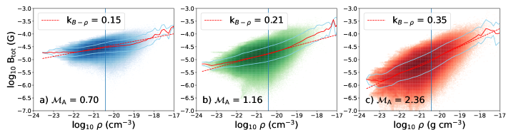
Figure 4: Fitting the slope of B-$\rho$ relation in log-log space. The a, b, and c panels display the B-$\rho$ distribution of simulations with $\beta$ = 0.2, 2, and 20, respectively. The red solid lines show the average B-$\rho$ relation and the blue lines show the dispersion region of the average B-$\rho$ relation. The red dashed lines are linear equations fitting the average B-$\rho$ relation. The blue perpendicular lines present the mean density $\bar{\rho}$. The slope of the $B-\rho$ relation is fitted around the mean density of the simulation as 0.15, 0.21, and 0.35, respectively.

Fig. 4 show the distribution between B-field and density in simulation with ${\cal M}_{\rm A}$ = 0.31, 0.49, 1.29, respectively. Fitting the main structure of $B-\rho$ distribution at the main density range of simulation in log-log space, the slope of $B-\rho$ relation, ${\rm d(log_{10}B)}/{\rm d(log_{10}\rho)}$ in simulations (${\cal M}_{\rm A}$ = 0.31, 0.49, 1.29) can be derived as 0.15, 0.21, 0.35, respectively.

table, with all parameters, energy ratios,

Appendix D Calculated the Slope of $B-\rho$ relation in Observation

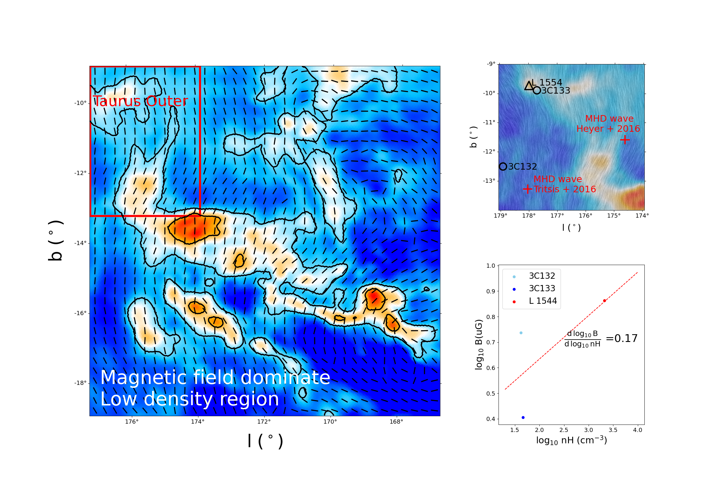
Figure 5: Fitting $B-\rho$ slope of Taurus outer region. The left panel displays the magnetic field of Taurus derived by Planck 353 GHz dust polarization (Planck Collaboration et al., 2020). The contours show the region where column density is above 2$\times$ 10²¹ cm^-2. Other region, column density $\textless$ 2$\times$ 10²¹ cm^-2, could exist the MHD wave (Heyer et al., 2016). The red region shows the Taurus outer region we used in this work. The right top panel shows the magnetic field morphology of the Taurus outer region and the position of distribution of 3C132, 3C133, and L1544. The right bottom panel displays the sources measured with the Zeeman effect located at the Taurus outer region, 3C132, 3C133, and L1544 in B-nH space, which show the mean magnetic field B and mean H₂ volume density nH (Crutcher et al., 2010; Ching et al., 2022). The right panel shows the positions of sources measured with Zeeman effect, 3C132, 3C133, TMC-1, and L1544 in l-b space (Heiles & Troland, 2004; Troland & Crutcher, 2008). The crosses show the candidate of MHD wave sources in the Taurus outer region (Heyer et al., 2016; Tritsis & Tassis, 2016).

Calculating Slope of $B-\rho$ relation have two method:
i) Single source with various scales
ii) Single source with various densities

D.1 Single source with various scales

The B-field $B$ and density $\rho$ of a single source is observed at various scales, such as NGC 6334 (Li et al., 2015)(${\rm d(log_{10}B)}/{\rm d(log_{10}\rho)}$ = 0.41).

D.2 Single source with various densities

The region of a single source has sub-regions with various densities. For example, the diffuse region (N(H₂) $\textless$ 2$\times$ 10²² cm^-2) in the Taurus could exist MHD wave (Heyer et al., 2016). As Fig. 5 shows, the Taurus out region has sub-areas with various densities, 3C132, 3C133, L1544 (Heyer et al., 2016; Tritsis & Tassis, 2016). Zeeman source 3C132 is located in the MHD Wave region and 3C133, L1544 is located at the boundary line of the MHD Wave region. (Ching et al., 2022) found that L1544 exists as the transition point between strong and weak magnetic fields. Fig. 5 shows the distribution between the mean density and mean B-field of three sources, which mean $\rho$ and $B$ come from (Collins et al., 2010; Ching et al., 2022). The slope of the $B-\rho$ relation in the Taurus outer region is fitting as 0.17.

Appendix E Energy Spectrum $\And$ Velocity Dispersion

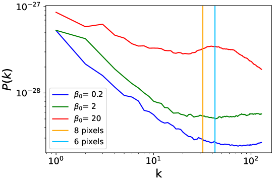
Figure 6: Energy spectrum of density in situations with various $\beta_{0}$. The blue, green, and red lines show the energy spectrum of density with $\beta_{0}$ as 0.2, 2, and 20, respectively. The orange and vertical blue lines display the structure on the scale of 8, and 20, respectively.

The energy spectrum of density $\rho$ in three simulations presents the density structure focused on the 6-pixel scale (see Fig. 6). We use the 8-pixel as the sub-block size to calculate the velocity dispersion $\sigma_{v}$ in each pixel of simulation data, which is close to the 6-pixel scale and can divide the whole scale of simulation data (256 pixels) without remainder:

$$v_{ijk,m}=\frac{\sum v_{ijk}\cdot\rho}{\sum\rho}\sum v_{ijk}$$ (E1)

$$\sigma_{v}=(\sum(v_{ijk}-v_{ijk,m})^{2})^{\frac{1}{2}}$$ (E2)

where the i,j,k show the axis of x,y, and z. The velocity dispersion can be used to compute the kinetic energy density ($e_{k}=\frac{1}{2}\rho\sigma_{v}^{2}$).

References

- Arzoumanian et al. (2021) Arzoumanian, D., Furuya, R. S., Hasegawa, T., et al. 2021, aap, 647, A78, doi: 10.1051/0004-6361/202038624
- Bryan et al. (1995) Bryan, G. L., Norman, M. L., Stone, J. M., Cen, R., & Ostriker, J. P. 1995, Computer Physics Communications, 89, 149, doi: 10.1016/0010-4655(94)00191-4
- Burkhart et al. (2015) Burkhart, B., Collins, D. C., & Lazarian, A. 2015, apj, 808, 48, doi: 10.1088/0004-637X/808/1/48
- Burkhart et al. (2020) Burkhart, B., Appel, S. M., Bialy, S., et al. 2020, apj, 905, 14, doi: 10.3847/1538-4357/abc484
- Cao & Li (2023) Cao, Z., & Li, H.-b. 2023, apjl, 946, L46, doi: 10.3847/2041-8213/acc5e8
- Ching et al. (2022) Ching, T. C., Li, D., Heiles, C., et al. 2022, nat, 601, 49, doi: 10.1038/s41586-021-04159-x
- Collins et al. (2012) Collins, D. C., Kritsuk, A. G., Padoan, P., et al. 2012, apj, 750, 13, doi: 10.1088/0004-637X/750/1/13
- Collins et al. (2010) Collins, D. C., Xu, H., Norman, M. L., Li, H., & Li, S. 2010, apjs, 186, 308, doi: 10.1088/0067-0049/186/2/308
- Crutcher et al. (2004) Crutcher, R. M., Nutter, D. J., Ward-Thompson, D., & Kirk, J. M. 2004, apj, 600, 279, doi: 10.1086/379705
- Crutcher et al. (2010) Crutcher, R. M., Wandelt, B., Heiles, C., Falgarone, E., & Troland, T. H. 2010, apj, 725, 466, doi: 10.1088/0004-637X/725/1/466
- Heiles & Troland (2004) Heiles, C., & Troland, T. H. 2004, apjs, 151, 271, doi: 10.1086/381753
- Heyer et al. (2016) Heyer, M., Goldsmith, P. F., Yıldız, U. A., et al. 2016, mnras, 461, 3918, doi: 10.1093/mnras/stw1567
- Hull et al. (2014) Hull, C. L. H., Plambeck, R. L., Kwon, W., et al. 2014, apjs, 213, 13, doi: 10.1088/0067-0049/213/1/13
- Jiang et al. (2020) Jiang, H., Li, H.-b., & Fan, X. 2020, apj, 890, 153, doi: 10.3847/1538-4357/ab672b
- Kandori et al. (2018) Kandori, R., Tomisaka, K., Tamura, M., et al. 2018, apj, 865, 121, doi: 10.3847/1538-4357/aadb3f
- Koch et al. (2018) Koch, P. M., Tang, Y.-W., Ho, P. T. P., et al. 2018, apj, 855, 39, doi: 10.3847/1538-4357/aaa4c1
- Konstantinou et al. (2024) Konstantinou, A., Ntormousi, E., Tassis, K., & Pallottini, A. 2024, arXiv e-prints, arXiv:2402.10268, doi: 10.48550/arXiv.2402.10268
- Li & Burkert (2018) Li, G.-X., & Burkert, A. 2018, mnras, 474, 2167, doi: 10.1093/mnras/stx2827
- Li (2021) Li, H.-B. 2021, Galaxies, 9, 41, doi: 10.3390/galaxies9020041
- Li et al. (2015) Li, H.-B., Yuen, K. H., Otto, F., et al. 2015, nat, 520, 518, doi: 10.1038/nature14291
- Matthews et al. (2009) Matthews, B. C., McPhee, C. A., Fissel, L. M., & Curran, R. L. 2009, apjs, 182, 143, doi: 10.1088/0067-0049/182/1/143
- Nakano (1978) Nakano, T. 1978, pasj, 30, 681
- O’Shea et al. (2004) O’Shea, B. W., Bryan, G., Bordner, J., et al. 2004, arXiv e-prints, astro, doi: 10.48550/arXiv.astro-ph/0403044
- Pattle et al. (2023) Pattle, K., Fissel, L., Tahani, M., Liu, T., & Ntormousi, E. 2023, in Astronomical Society of the Pacific Conference Series, Vol. 534, Protostars and Planets VII, ed. S. Inutsuka, Y. Aikawa, T. Muto, K. Tomida, & M. Tamura, 193, doi: 10.48550/arXiv.2203.11179
- Planck Collaboration et al. (2020) Planck Collaboration, Aghanim, N., Akrami, Y., et al. 2020, aap, 641, A12, doi: 10.1051/0004-6361/201833885
- Schneider et al. (2022) Schneider, N., Ossenkopf-Okada, V., Clarke, S., et al. 2022, aap, 666, A165, doi: 10.1051/0004-6361/202039610
- Tritsis & Tassis (2016) Tritsis, A., & Tassis, K. 2016, mnras, 462, 3602, doi: 10.1093/mnras/stw1881
- Tritsis & Tassis (2018) —. 2018, Science, 360, 635, doi: 10.1126/science.aao1185
- Troland & Crutcher (2008) Troland, T. H., & Crutcher, R. M. 2008, apj, 680, 457, doi: 10.1086/587546
- Ustyugov et al. (2009) Ustyugov, S. D., Popov, M. V., Kritsuk, A. G., & Norman, M. L. 2009, Journal of Computational Physics, 228, 7614, doi: 10.1016/j.jcp.2009.07.007
- Wang et al. (2020) Wang, J.-W., Lai, S.-P., Clemens, D. P., et al. 2020, apj, 888, 13, doi: 10.3847/1538-4357/ab5c1c
- Yang et al. (2023) Yang, R.-z., Li, G.-X., Wilhelmi, E. d. O., et al. 2023, Nature Astronomy, 7, 351, doi: 10.1038/s41550-022-01868-9
- Zhang et al. (2019) Zhang, Y., Guo, Z., Wang, H. H., & Li, H. b. 2019, apj, 871, 98, doi: 10.3847/1538-4357/aaf57c