Unifying Causal Representation Learning with the Invariance Principle

Abstract

Causal representation learning aims at recovering latent causal variables from high-dimensional observations to solve causal downstream tasks, such as predicting the effect of new interventions or more robust classification. A plethora of methods have been developed, each tackling carefully crafted problem settings that lead to different types of identifiability. The folklore is that these different settings are important, as they are often linked to different rungs of Pearl’s causal hierarchy, although not all neatly fit. Our main contribution is to show that many existing causal representation learning approaches methodologically align the representation to known data symmetries. Identification of the variables is guided by equivalence classes across different “data pockets” that are not necessarily causal. This result suggests important implications, allowing us to unify many existing approaches in a single method that can mix and match different assumptions, including non-causal ones, based on the invariances relevant to our application. It also significantly benefits applicability, which we demonstrate by improving treatment effect estimation on real-world high-dimensional ecological data. Overall, this paper clarifies the role of causality assumptions in the discovery of causal variables and shifts the focus to preserving data symmetries.

1 Introduction

Causal representation learning (Schölkopf et al., 2021) posits that many real-world high-dimensional perceptual data can be described through a simplified latent structure specified by a few interpretable low-dimensional causally-related variables. Discovering hidden causal structures from data has been a long-standing goal across many scientific disciplines, spanning neuroscience (Vigário et al., 1997; Brown et al., 2001), communication theory (Ristaniemi, 1999; Donoho, 2006), economics (Angrist and Pischke, 2009) and social science (Antonakis and Lalive, 2011). From the machine learning perspective, algorithms and models integrated with causal structure are often proven to be more robust at distribution shift (Ahuja et al., 2022a; Bareinboim and Pearl, 2016; Rojas-Carulla et al., 2018), providing better out-of-distribution generalization results and reliable agent planning (Fumero et al., 2024; Seitzer et al., 2021; Urpí et al., 2024). Formally, the general goal of causal representation learning approaches is formulated as to provably identify ground-truth latent causal variables and their causal relations (up to certain ambiguities).

Many existing approaches in causal representation learning carefully formulate their problem settings to guarantee identifiability and justify the assumptions within the framework of Pearl’s causal hierarchy, such as “observational, interventional, or counterfactual CRL" (von Kügelgen et al., 2024; Ahuja et al., 2023; Brehmer et al., 2022; Buchholz et al., 2023; Zhang et al., 2024a; Varici et al., 2024a). However, some causal representation learning works may not perfectly fit within this causal language framework; for instance, the problem setting of temporal CRL works (Lachapelle et al., 2022; Lippe et al., 2022a, b, 2023) does not always align straightforwardly with existing categories. They often assume that an individual trajectory is “intervened” upon, but this is not an intervention in the traditional sense, as noise variables are not resampled. It is also not a counterfactual as the value of non-intervened variables can change due to default dynamics. Similarly, domain generalization (Sagawa et al., 2019; Krueger et al., 2021; Ahuja et al., 2022a) and certain multi-task learning approaches (Lachapelle et al., 2023; Fumero et al., 2024) are sometimes framed as informally related to causal representation learning. However, the precise relation to causality is not always clearly articulated. This has resulted in a variety of methods and findings, some of which rely on assumptions that might be too narrowly tailored for practical, real-world applications. For example, Cadei et al. (2024) collected a data set for estimating treatment effects from high-dimensional observations in real-world ecology experiments. Despite the clear causal focus of the benchmark, they note that, despite having access to multiple views and being able to perform some interventions, neither existing mutli-view nor intervertional causal representation learning methods are directly applicable due to mismatching assumptions.

This paper contributes a unified rephrasing of many existing nonparametric CRL works through the lens of invariance. We observe that many existing causal representation approaches share methodological similarities, particularly in aligning the representation with known data symmetries, while differing primarily in how the invariance principle is invoked. This invariance principle is usually formulated implicitly in the assumed data-generating process. Instead, we make this explicit and show that latent causal variable identification broadly originates from multiple data pockets with certain underlying equivalence relations. These are not necessarily causal and (with minor exceptions) have to be known apriori. Unifying causal representation learning approaches using the invariance principle brings several potential benefits: First, it helps clarify the alignment between seemingly different categories of CRL methods, contributing to a more coherent and accessible framework for understanding causal representation learning. This perspective may also allow for the integration of multiple invariance relations in latent variable identification, which could improve the flexibility of these methods in certain practical settings. Additionally, our theory underscores a gap in the necessary causal assumptions for graph learning, which is essential for generalizing to unseen interventions and helps distinguish it from the problem of identifying causal variables. These invariances can be expressed in causal terms, such as interventions, but do not always need to be. Last but not least, this formulation of invariance relation links causal representation learning to many existing representation learning areas outside of causality, including invariant training (Arjovsky et al., 2020; Ahuja et al., 2022a), domain adaptation (Sagawa et al., 2019; Krueger et al., 2021), and geometric deep learning  (Cohen and Welling, 2016; Bronstein et al., 2017, 2021).

We highlight our contributions as follows:

1. We propose a unified rephrasing for existing nonparmaetric causal representation learning approaches leveraging the invariance principles and prove latent variable identifiability in this general setting. We show that 31 existing identification results can be seen as special cases directly implied by our framework. This approach also enables us to derive new results, including latent variable identifiability from one imperfect intervention per node in the non-parametric setting.

2. In addition to employing different methods, many works in the CRL literature use varying definitions of “identifiability." We formalize these definitions at different levels of granularity, highlight their connections, and demonstrate how various definitions can be addressed within our framework by leveraging different invariance principles.

3. Upon the identifiability of the latent variables, we discuss the necessary causal assumptions for graph identification and the possibility of partial graph identification using the language of causal consistency. With this, we draw a distinction between the causal assumptions necessary for graph discovery and those that may not be required for variable discovery.

4. Our framework is broadly applicable across a range of settings. We observe improved results on real-world experimental ecology data using the causal inference benchmark from high-dimensional observations provided by Cadei et al. (2024). Additionally, we present a synthetic ablation to demonstrate that existing methods, which assume access to interventions, actually only require a form of distributional invariance to identify variables. This invariance does not necessarily need to correspond to a valid causal intervention.

2 Problem Setting

This section formalizes our problem setting and states our main assumptions. We first summarize standard definitions and assumptions of causal representation learning in § 2.1. Then, we describe the data generating process using the language of invariance properties and equivalence classes (§ 2.2).

Notation. $[N]$ is used as a shorthand for $\{1,\dots,N\}$. We use bold lower-case $\mathbf{z}$ for random vectors and normal lower-case $z$ for their realizations. A vector $\mathbf{z}$ can be indexed either by a single index $i\in[\dim(\mathbf{z})]$ via $\mathbf{z}_{i}$ or a index subset $A\subseteq[\dim(\mathbf{z})]$ with $\mathbf{z}_{A}:=\{\mathbf{z}_{i}:i\in A\}$. $P_{\mathbf{z}}$ denotes the probability distribution of the random vector $\mathbf{z}$ and $p_{\mathbf{z}}(z)$ denotes the associated probability density function. By default, a "measurable" function is measurable w.r.t. the Borel sigma algebras and defined w.r.t. the Lebesgue measure. A more comprehensive summary of notations and terminologies is provided in App. A

2.1 Preliminaries

In this subsection, we revisit the common definitions and assumptions in identifiability works from causal representation learning. We begin with the definition of a latent structural causal model:

Definition 2.1 (Latent SCM (von Kügelgen et al., 2024)).

Let $\mathbf{z}=\{\mathbf{z}_{1},\dots,\mathbf{z}_{N}\}$ denote a set of causal “endogenous" variables with each $\mathbf{z}_{i}$ taking values in $\mathbb{R}$, and let $\mathbf{u}=\{\mathbf{u}_{1},\dots,\mathbf{u}_{N}\}$ denotes a set of mutually independent “exogenous" random variables. The latent SCM consists of a set of structural equations

$$\{\mathbf{z}_{i}:=m_{i}(\mathbf{z}_{\text{pa}(i)}),\mathbf{u}_{i}\}_{i=1}^{N},$$ (2.1)

where $\mathbf{z}_{\text{pa}(i)}$ are the causal parents of $\mathbf{z}_{i}$ and $m_{i}$ are the deterministic functions that are termed “causal mechanisms". We indicate with $P_{\mathbf{u}}$ the joint distribution of the exogenous random variables, which due to the independence hypothesis is the product of the probability measures of the individual variables. The associated causal diagram $\mathcal{G}$ is a directed graph with vertices $\mathbf{z}$ and edges $\mathbf{z}_{i}\to\mathbf{z}_{j}$ iff. $\mathbf{z}_{i}\in\mathbf{z}_{\text{pa}(j)}$; we assume the graph $\mathcal{G}$ to be acyclic.

The latent SCM induces a unique distribution $P_{\mathbf{z}}$ over the endogenous variables $\mathbf{z}$ as a pushforward of $P_{\mathbf{u}}$ via eq. 2.1. Its density $p_{\mathbf{z}}$ follows the causal Markov factorization:

$$p_{\mathbf{z}}(z)=\prod_{i=1}^{N}p_{i}(z_{i}~{}|~{}{z}_{\text{pa}({i})})$$ (2.2)

Instead of directly observing the endogenous and exogenous variables $\mathbf{z}$ and $\mathbf{u}$, we only have access to some “entangled" measurements $\mathbf{x}$ of $\mathbf{z}$ generated through a nonlinear mixing function:

Definition 2.2 (Mixing function).

A deterministic smooth function $f:\mathbb{R}^{N}\to\mathbb{R}^{D}$ mapping the latent vector $\mathbf{z}\in\mathbb{R}^{N}$ to its observable $\mathbf{x}\in\mathbb{R}^{D}$, where $D\geq N$ denotes the dimensionality of the observational space.

Assumption 2.1 (Diffeomorphism).

The mixing function $f$ is diffeomorphic onto its image, i.e. $f$ is $C^{\infty}$, $f$ is injective and $f^{-1}|_{\mathcal{I}(f)}:\mathcal{I}(f)\rightarrow\mathbb{R}^{D}$ is also $C^{\infty}$.

Remark: Settings with noisy observations ($\mathbf{x}=f(\mathbf{z})+\epsilon,\,\mathbf{z}\perp\epsilon$) can be easily reduced to our denoised version by applying a standard deconvolution argument as a pre-processing step, as indicated by Lachapelle et al. (2022); Buchholz et al. (2023).

2.2 Data Generating Process

We now define our data generating process using the previously introduced mathematical framework  (§ 2.1). Unlike prior works in causal representation learning, which typically categorize their settings using established causal language (such as ’counterfactual,’ ’interventional,’ or ’observational’), our approach introduces a more general invariance principle that aims to unify diverse problem settings. In the following, we introduce the following concepts as mathematical tools to describe our data generating process.

Definition 2.3 (Invariance property).

Let $A\subseteq[N]$ be an index subset of the Euclidean space $\mathbb{R}^{N}$ and let $\sim_{\iota}$ be an equivalence relationship on $\mathbb{R}^{|A|}$, with $A$ of known dimension. Let $\mathcal{M}:={\raisebox{1.99997pt}{$\mathbb{R}^{|A|}$}\left/\raisebox{-1.99997pt}{$\sim_{\iota}$}\right.}$ be the quotient of $\mathbb{R}^{|A|}$ under this equivalence relationship; $\mathcal{M}$ is a topological space equipped with the quotient topology. Let $\iota:\mathbb{R}^{|A|}\to\mathcal{M}$ be the projection onto the quotient induced by the equivalence relationship $\sim_{\iota}$. We call this projection $\iota$ the invariant property of this equivalence relation. We say that two vectors $\mathbf{a},\mathbf{b}\in\mathbb{R}^{|A|}$ are invariant under $\iota$ if and only if they belong to the same $\sim_{\iota}$ equivalence class, i.e.:

$$\iota(\mathbf{a})=\iota(\mathbf{b})\Leftrightarrow\mathbf{a}\sim_{\iota}\mathbf{b}.$$

Extending this definition to the whole latent space $\mathbb{R}^{N}$, a pair of latents $\mathbf{z},\tilde{\mathbf{z}}\in\mathbb{R}^{N}$ are non-trivially invariant on a subset $A\subseteq[N]$ under the property $\iota$ only if

1. the invariance property $\iota$ holds on the index subset $A\subseteq[N]$ in the sense that $\iota(\mathbf{z}_{A})=\iota(\tilde{\mathbf{z}}_{A})$;

2. for any smooth function $h_{1},h_{2}:\mathbb{R}^{N}\to\mathbb{R}^{|A|}$, the invariance property between $\mathbf{z},\tilde{\mathbf{z}}$ breaks under the $h_{1},h_{2}$ transformations if $h_{1}$ or $h_{2}$ directly depends on some other component $\mathbf{z}_{q}$ with $q\in[N]\setminus A$. Taking $h_{1}$ and $\mathbf{z}$ as an example, we have:

   $$\exists q\in{[N]\setminus A},\mathbf{z}^{*}\in\mathbb{R}^{N},\quad s.t.\ \dfrac{\partial{h_{1}}}{\partial{\mathbf{z}_{q}}}(\mathbf{z}^{*})\text{ exists and is non zero}\quad\Rightarrow\quad\iota(h_{1}(\mathbf{z}))\neq\iota(h_{2}(\tilde{\mathbf{z}}))$$ (2.3)

   which means: given that the partial derivative of $h_{1}$ w.r.t. some latent variable $\mathbf{z}_{q}\in\mathbf{z}_{[N]\setminus A}$ is non-zero at some point $\mathbf{z}^{*}\in\mathbb{R}^{N}$, $h_{1}(\mathbf{z}),h_{2}(\mathbf{z})$ violates invariance principle in the sense that $\iota(h_{1}(\mathbf{z}))\neq\iota(h_{2}(\tilde{\mathbf{z}}))$. That is, the invariance principle is non-trivial in the sense of not being always satisfied.

Remark:  Defn. 2.3 (ii) is essential for latent variable identification on the invariant partition $A$, which is further justified in LABEL:app:ass_justification by showing a non-identifiable example violating (ii). Intuitively, Defn. 2.3 (ii) present sufficient discrepancy between the invariant and variant part in the ground truth generating process, paralleling various key assumptions for identifiability in CRL that were termed differently but conceptually similar, such as sufficient variability (von Kügelgen et al., 2024; Lippe et al., 2022b), interventional regularity (Varici et al., 2023, 2024b) and interventional discrepancy (Liang et al., 2023; Varici et al., 2024a). On a high level, these assumptions guarantee that the intervened mechanism sufficiently differs from the default causal mechanism to effectively distinguish the intervened and non-intervened latent variables, which serves the same purpose as  Defn. 2.3 (ii). We elaborate this link further in LABEL:app:ass_justification.

We denote by ${\mathcal{S}}_{\mathbf{z}}:=\{\mathbf{z}^{1},\dots,\mathbf{z}^{K}\}$ the set of latent random vectors with $\mathbf{z}^{k}\in\mathbb{R}^{N}$ and write its joint distribution as $P_{{\mathcal{S}}_{\mathbf{z}}}$. The joint distribution $P_{{\mathcal{S}}_{\mathbf{z}}}$ has a probability density $p_{{\mathcal{S}}_{\mathbf{z}}}(z^{1},\dots,z^{K})$. Each individual random vector $\mathbf{z}^{k}\in{\mathcal{S}}_{\mathbf{z}}$ follows the marginal density $p_{\mathbf{z}^{k}}$ with the non-degenerate support $\mathcal{Z}^{k}\subseteq\mathbb{R}^{N}$, whose interion is a non-empty open set of $\mathbb{R}^{N}$.

Definition 2.4 (Observable of a set of latent random vectors).

Consider a set of random vectors ${\mathcal{S}}_{\mathbf{z}}:=\{\mathbf{z}^{1},\dots,\mathbf{z}^{K}\}$ with $\mathbf{z}^{k}\in\mathbb{R}^{N}$, the corresponding set of observables ${\mathcal{S}}_{\mathbf{x}}:=\{\mathbf{x}^{1},\dots,\mathbf{x}^{K}\}$ is generated by:

$${\mathcal{S}}_{\mathbf{x}}=F({\mathcal{S}}_{\mathbf{z}}),$$ (2.4)

where the map $F$ defines a push-forward measure $F_{\#}(P_{{\mathcal{S}}_{\mathbf{z}}})$ on the image of $F$ as:

$$F_{\#}(P_{{\mathcal{S}}_{\mathbf{z}}})(x_{1},\dots,x_{K})=P_{{\mathcal{S}}_{\mathbf{z}}}(f_{1}^{-1}(x_{1}),\dots,f_{K}^{-1}(x_{K}))$$ (2.5)

with the support $\mathcal{X}:=\text{Im}(F)\subseteq\mathbb{R}^{K\times D}$. Note that $F$ satisfies Asm. 2.1 as each $f_{k}$ is a diffeomorphism onto its image according to Asm. 2.1.

In the following, we denote by $\mathfrak{I}:=\{\iota_{i}:\mathbb{R}^{|A_{i}|}\to\mathcal{M}_{i}\}$ a finite set of invariance properties with their respective invariant subsets $A_{i}\subseteq[N]$ and their equivalence relationships $\sim_{\iota_{i}}$, each inducing as a projection onto its quotient and invariant property $\iota_{i}$ (Defn. 2.3). For a set of observables ${\mathcal{S}}_{\mathbf{x}}:=\{\mathbf{x}^{1},\dots,\mathbf{x}^{K}\}\in\mathcal{X}$ generated from the data generating process described in § 2.2, we assume:

Assumption 2.2.

For each $\iota_{i}\in\mathfrak{I}$, there exists a unique known index subset $V_{i}\subseteq[K]$ with at least two elements (i.e., $|V_{i}|\geq 2)$ s.t. $\mathbf{x}_{V_{i}}=F([\mathbf{z}]_{\sim_{\iota_{i}}})$ forms the set of observables generated from an equivalence class $[\mathbf{z}]_{\sim_{\iota_{i}}}:=\{\tilde{\mathbf{z}}\in\mathbb{R}^{N}:\mathbf{z}_{A_{i}}\sim_{\iota_{i}}\tilde{\mathbf{z}}_{A_{i}}\}$, as given by Defn. 2.4. In particular, if $\mathfrak{I}=\{\iota\}$ consists of a single invariance property $\iota:\mathbb{R}^{|A|}\to\mathcal{M}$, we have ${\mathcal{S}}_{\mathbf{x}}=F([\mathbf{z}]_{\sim_{\iota}})$.

Remark: While $\mathfrak{I}$ does not need to be fully described, which observables should belong to the same equivalence class is known (denoted as $V_{i}\subseteq[K]$ for the invariance property $\iota_{i}\in\mathfrak{I}$). This is a standard assumption and is equivalent to knowing e.g., two views are generated from partially overlapped latents (Yao et al., 2023).

3 Identifiability Theory via the Invariance Principle

This section contains our main identifiability results using the invariance principle, i.e., to align the learned representation with known data symmetries. First, we present a general proof for latent variable identification that brings together many identifiability results from existing CRL works, including multiview, interventional, temporal, and multitask CRL. We compare different granularity of latent variable identification and show their transitions through certain assumptions on the causal model or mixing function (§ 3.1). Afterward, we discuss the identification level of a causal graph depending on the granularity of latent variable identification under certain structural assumptions (§ 3.3). Detailed proofs are deferred to LABEL:app:proofs.

3.1 Identifying latent variables

High-level overview. Our general theory of latent variable identifiability, based on the invariance principle, consists of two key components: (1) ensuring the encoder’s sufficiency, thereby obtaining an adequate representation of the original input for the desired task; (2) guaranteeing the learned representation to preserve known data symmetries as invariance properties. The sufficiency is often enforced by minimizing the reconstruction loss  (Locatello et al., 2020; Ahuja et al., 2022b; Lippe et al., 2022b, a; Lachapelle et al., 2022) in auto-encoder based architecture, maximizing the log likelihood in normalizing flows or maximizing entropy (Zimmermann et al., 2021; von Kügelgen et al., 2021; Daunhawer et al., 2023; Yao et al., 2023) in contrastive-learning based approaches. The invariance property in the learned representations is often enforced by minimizing some equivalence relation-induced pseudometric between a pair of encodings (von Kügelgen et al., 2021; Yao et al., 2023; Lippe et al., 2022b; Zhang et al., 2024a) or by some iterative algorithm that provably ensures the invariance property on the output (Squires et al., 2023; Varici et al., 2024b). As a result, all invariant blocks $A_{i},i\in[n_{\mathfrak{I}}]$ can be identified up to a mixing within the blocks while being disentangled from the rest. This type of identifiability is defined as block-identifiability (von Kügelgen et al., 2021) which we restate as follows:

Definition 3.1 (Block-identifiability (von Kügelgen et al., 2021)).

A subset of latent variable $\mathbf{z}_{A}:=\{\mathbf{z}_{j}\}_{j\in A}$ with $A\subseteq[N]$ is block-identified by an encoder $g:\mathbb{R}^{D}\to\mathbb{R}^{N}$ on the invariant subset $A$ if the learned representation $\hat{\mathbf{z}}_{\hat{A}}:=[g(\mathbf{x})]_{\hat{A}}$ with $\hat{A}\subseteq[N],|A|=|\hat{A}|$ contains all and only information about the ground truth $\mathbf{z}_{A}$, i.e. $\hat{\mathbf{z}}_{\hat{A}}=h(\mathbf{z}_{A})$ for some diffeomorphism $h:\mathbb{R}^{|A|}\to\mathbb{R}^{|A|}$.

Definition 3.2 (Encoders).

The encoders $G:=\{g_{k}:\mathcal{X}^{k}\to\mathcal{Z}^{k}\}_{k\in[K]}$ consist of smooth functions mapping from the respective observational support $\mathcal{X}^{k}$ to the corresponding latent support $\mathcal{Z}^{k}$, as elaborated in § 2.2.

Definition 3.3 (Selection (Yao et al., 2023)).

A selection $\oslash$ operates between two vectors $a\in\{0,1\}^{d}\,,b\in\mathbb{R}^{d}$ s.t.

$$\textstyle a\oslash b:=[b_{j}:a_{j}=1,j\in[d]]$$

Definition 3.4 (Invariant block selectors).

The invariant block selectors $\Phi:=\{\phi^{(i,k)}\}_{i\in[n_{\mathfrak{I}}],k\in V_{i}}$ with $\phi^{(i,k)}\in\{0,1\}^{N}$ perform selection (Defn. 3.3) on the encoded information: for any invariance property $\iota_{i}\in\mathfrak{I}$, any observable $\mathbf{x}^{k},k\in V_{i}$ we have the selected representation:

$$\textstyle\phi^{(i,k)}\oslash\hat{\mathbf{z}}^{k}=\phi^{(i,k)}\oslash g_{k}(\mathbf{x}^{k})=\left[[g_{k}(\mathbf{x}^{k})]_{j}:\phi^{(i,k)}_{j}=1,j\in[N]\right],$$ (3.1)

with $\left\lVert\phi^{(i,k)}\right\rVert_{0}=\|\phi^{(i,k^{\prime})}\|_{0}=|A_{i}|$ for all $\iota_{i}\in\mathfrak{I},k,k^{\prime}\in V_{i}$.

Constraint 3.1 (Invariance constraint).

For any $\iota_{i}\in\mathfrak{I},i\in[n_{\mathfrak{I}}]$, the selected representations $\phi^{(i,k)}\oslash g_{k}(\mathbf{x}^{k}),k\in[K]$ must be $\iota_{i}$-invariant across the observables from the subset $V_{i}\subset[K]$:

$$\iota_{i}(\phi^{(i,k)}\oslash g_{k}(\mathbf{x}^{k}))=\iota_{i}(\phi^{(i,k^{\prime})}\oslash g_{k^{\prime}}(\mathbf{x}^{k^{\prime}}))\quad\forall i\in[n_{\mathfrak{I}}]\,\,\forall k,k^{\prime}\in V_{i}$$ (3.2)

Constraint 3.2 (Sufficiency constraint).

For any encoder $g_{k},k\in[K]$, the learned representation preserves at least as much information as of any of the invariant partitions $\mathbf{z}_{A_{i}}$ that we aim to identify in the sense that $I(\mathbf{z}_{A_{i}},g_{k}(\mathbf{x}^{k}))=H(\mathbf{z}_{A_{i}})\quad\forall i\in[n_{\mathfrak{I}}],k\in V_{i}$.

Theorem 3.1 (Identifiability of multiple invariant blocks).

Consider a set of observables ${\mathcal{S}}_{\mathbf{x}}=\{\mathbf{x}^{1},\mathbf{x}^{2},\dots,\mathbf{x}^{K}\}$ with $\mathbf{x}^{k}\in\mathcal{X}^{k}$ generated from § 2.2 satisfying Asm. 2.2. Let $G,\Phi$ be the set of smooth encoders (Defn. 3.2) and selectors (Defn. 3.4) that satisfy Constraints 3.1 and 3.2, then the invariant component $\mathbf{z}_{A_{i}}^{k}$ is block-identified (Defn. 3.1) by $\phi^{(i,k)}\oslash g_{k}$ for all $\iota_{i}\in\mathfrak{I},k\in[K]$.

What about the variant latents? Intuitively, the variant latents are generally not identifiable, as the invariance constraint (Constraint 3.1) is applied only to the selected invariant encodings, leaving the variant part without any weak supervision (Locatello et al., 2019). This non-identifiability result is formalized as follows:

Proposition 3.2 (General non-identifiability of variant latent variables).

Consider the setup in Thm. 3.1, let $A:=\bigcup_{i\in[n_{\mathfrak{I}}]}A_{i}$ denote the union of block-identified latent indexes and $A^{\mathrm{c}}:=[N]\setminus A$ the complementary set where no $\iota$-invariance $\iota\in\mathfrak{I}$ applies, then the variant latents $\mathbf{z}_{A^{\mathrm{c}}}$ cannot be identified.

Although variant latent variables are generally non-identifiable, they can be identified under certain conditions. The following demonstrates that variant latent variables can be identified under invertible encoders when the variant and invariant partitions are mutually independent.

Proposition 3.3 (Identifiability of variant latent under independence).

Consider an optimal encoder $g\in G^{*}$ and optimal selector $\phi\in\Phi^{*}$ from Thm. 3.1 that jointly identify an invariant block $\mathbf{z}_{A}$ (we omit subscriptions $k,i$ for simplicity), then $\mathbf{z}_{A^{\mathrm{c}}}(A^{\mathrm{c}}:=[N]\setminus A)$ can be identified by the complementary encoding partition $(1-\phi)\oslash g$ only if

1. $g$ is invertible in the sense that $I(\mathbf{x},g(\mathbf{x}))=H(\mathbf{x})$;

2. $\mathbf{z}_{A^{\mathrm{c}}}$ is independent on $\mathbf{z}_{A}$.

3.2 On the granularity of identification

Different levels of identification can be achieved depending on the degree of underlying data symmetry. Below, we present three standard identifiability definitions from the CRL literature, each offering stronger identification results than block-identifiability (Defn. 3.1).

Definition 3.5 (Block affine-identifiability).

Let $\hat{\mathbf{z}}$ be the learned representation, for a subset $A\subseteq[N]$ it satisfies that:

$$\hat{\mathbf{z}}_{\pi(A)}=D\cdot\mathbf{z}_{A}+\mathbf{b},$$ (3.3)

where $D\in\mathbb{R}^{|A|\times|A|}$ is an invertible matrix, $\pi(A)$ denotes the index permutation of $A$, then $\mathbf{z}_{A}$ is block affine-identified by $\hat{\mathbf{z}}_{\pi(A)}$.

Definition 3.6 (Element-identifiability).

The learned representation $\hat{\mathbf{z}}\in\mathbb{R}^{N}$ satisfies that:

$$\hat{\mathbf{z}}=\mathbf{P}_{\pi}\cdot h(\mathbf{z}),$$ (3.4)

where $\mathbf{P}_{\pi}\in\mathbb{R}^{N\times N}$ is a permutation matrix, $h(\mathbf{z}):=(h_{1}(\mathbf{z}_{1}),\dots h_{N}(\mathbf{z}_{N}))\in\mathbb{R}^{N}$ is a is an element-wise diffeomorphism.

Definition 3.7 (Affine-identifiability).

The learned representation $\hat{\mathbf{z}}\in\mathbb{R}^{N}$ satisfies that:

$$\hat{\mathbf{z}}=\Lambda\cdot\mathbf{P}_{\pi}\cdot\mathbf{z}+\mathbf{b},$$ (3.5)

where $\mathbf{P}_{\pi}\in\mathbb{R}^{N\times N}$ is a permutation matrix, $\Lambda\in\mathbb{R}^{N\times N}$ is a diagonal matrix with nonzero diagonal entries.

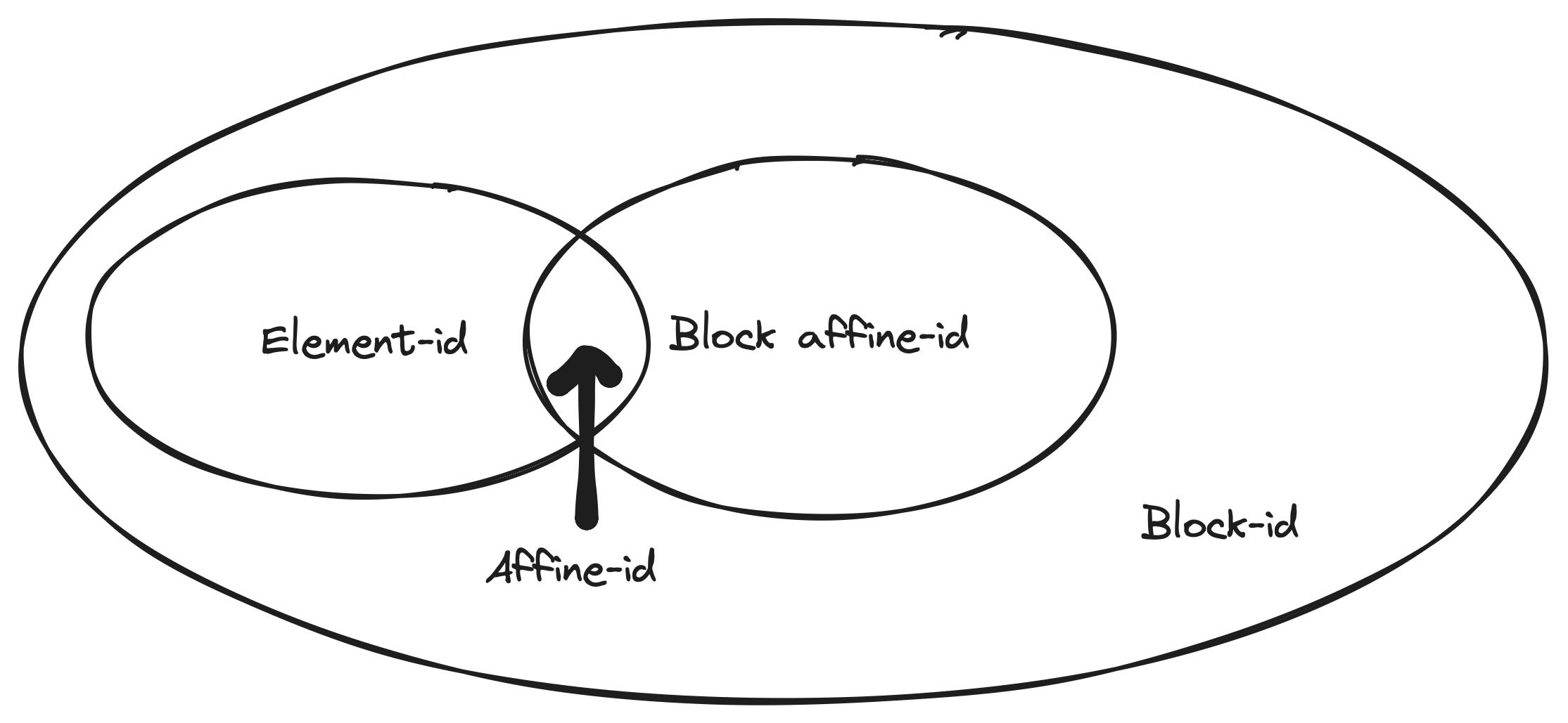
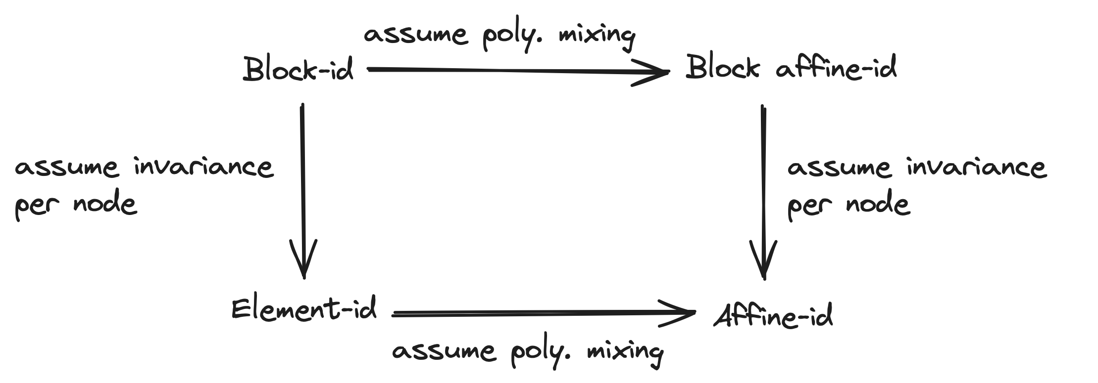
Figure 1: Relations between different identification classes (Defns. 3.1, 3.6, 3.7 and 3.5). Some CRL works proposed a more fine-grained classification of identifiability concepts with slightly different terminology, which we omit here for readability.

Proposition 3.4 (Granularity of identification).

Affine-identifiability (Defn. 3.7) implies element-identifiability (Defn. 3.6) and block affine-identifiability (Defn. 3.5) while element-identifiability and block affine-identifiability implies block-identifiability (Defn. 3.1).

Proposition 3.5 (Transition between identification levels).

The transition between different levels of latent variable identification (Fig. 1) can be summarized as follows:

1. Element-level identifiability (Defns. 3.6 and 3.7) can be obtained from block-wise identifiability (Defns. 3.5 and 3.1) when each individual latent constitutes an invariant block;

2. Identifiability up to an affine transformation (Defns. 3.5 and 3.7) can be obtained from general identifiability on arbitrary diffeomorphism (Defns. 3.6 and 3.1) by additionally assuming that both the ground truth mixing function and decoder are finite degree polynomials of the same degree.

3.3 Identifying the causal graph

In addition to latent variable identification, another goal of causal representation learning is to infer the underlying latent dependency, namely the causal graph structure. Hence, we restate the standard definition of graph identifiability in causal representation learning.

Definition 3.8 (Graph-identfiability).

The estimated graph $\hat{\mathcal{G}}$ is isomorphic to the ground truth $\mathcal{G}$ through a bijection $h:V(\mathcal{G})\to V(\hat{\mathcal{G}})$ in the sense that two vertices $\mathbf{z}_{i},\mathbf{z}_{j}\in V(\mathcal{G})$ are adjacent in $\mathcal{G}$ if and only if $h(\mathbf{z}_{i}),h(\mathbf{z}_{j})\in V(\hat{\mathcal{G}})$ are adjacent in $\hat{\mathcal{G}}$.

We remark that the “faithfulness" assumption (Pearl, 2009, Defn. 2.4.1) is a standard assumption in the CRL literature, commonly required for graph discovery. We restate it as follows:

Assumption 3.1 (Faithfulness (or Stability)).

$P_{\mathbf{z}}$ is a faithful distribution induced by the latent SCM (Defn. 2.1) in the sense that $P_{\mathbf{z}}$ contains no extraneous conditional independence; in other words, the only conditional independence relations satisfied by $P_{\mathbf{z}}$ are those given by $\{\mathbf{z}_{i}\perp{\mathbf{z}}_{\text{nd}({i})}~{}|~{}{\mathbf{z}}_{\text{pa}({i})}\}$ where ${\mathbf{z}}_{\text{nd}({i})}$ denotes the non-descends of $\mathbf{z}_{i}$.

As indicated by Defn. 3.8, the preliminary condition of identifying the causal graph is to have an element-wise correspondence between the vertices in the ground truth graph $\mathcal{G}$ (i.e., the ground truth latents) and the vertices of the estimated graph. Therefore, the following assumes that the learned encoders $G$ (Defn. 3.2) achieve element-identifiability (Defn. 3.6), that is, for each $\mathbf{z}_{i}\in\mathbf{z}$, we have a differmorphism $h_{i}:\mathbb{R}\to\mathbb{R}$ such that $\hat{\mathbf{z}}_{i}=h_{i}(\mathbf{z}_{i})$. However, to identify the graph structure, additional assumptions are needed: either on the source of invariance or on the parametric form of the latent causal model.

Graph identification via interventions. Under the element-identifiability (Defn. 3.6) of the latent variables $\mathbf{z}$, the causal graph structure $\mathcal{G}$ can be identified up to its isomorphism (Defn. 3.8), given multi-domain data from paired perfect interventions per-node  (von Kügelgen et al., 2024; Varici et al., 2024a). Using data generated from imperfect interventions is generally insufficient to identify the direct edges in the causal graph, it can only identify the ancestral relations, i.e., up to the transitive closure of $\mathcal{G}$ (Brehmer et al., 2022; Zhang et al., 2024a). Unfortunately, even imposing the linear assumption on the latent SCM does not provide a solution (Squires et al., 2023). Nevertheless, by adding sparsity assumptions on the causal graph $\mathcal{G}$ and polynomial assumption on the mixing function $f$,  Zhang et al. (2024a) has shown isomorphic graph identifiability (Defn. 3.8) under imperfect intervention per node. In general, access to the interventions is necessary for graph identification if one is not comfortable making other parametric assumptions about the graph structure. Conveniently, in this setting, the graph identifiability is linked with that of the variables since the latter leverages the invariance induced by the intervention.

Graph identification via parametric assumptions. It is well known in causal discovery that the additive noise model (Hoyer et al., 2008) is identifiable under certain mild assumptions (Zhang and Hyvärinen, 2010, 2009). In the following, we assume an additive exogenous noise in the latent SCM (Defn. 2.1):

Assumption 3.2 (Additive noise).

The endogenous variable $\mathbf{z}_{i}\in\mathbb{R}$ in the previously defined latent SCM (Defn. 2.1) relates to the corresponding exogenous noise variable $\mathbf{u}_{i}\in\mathbb{R}$ through additivity. Namely, the causal mechanism (eq. 2.1) can be rewritten as:

$$\{\mathbf{z}_{i}=m_{i}({\mathbf{z}}_{\text{pa}({i})})+\mathbf{u}_{i}\}.$$ (3.6)

As a generalization of the additive noise model, the post-nonlinear acyclic causal model (Zhang and Hyvärinen, 2010, Sec. 2) allows extra nonlinearity on the top of the additive causal mechanism, providing additional flexibility on the latent model assumption:

Definition 3.9 (Post-nonlinear acyclic causal model).

The following causal mechanism describes a post-nonlinear acyclic causal model:

$$\mathbf{z}_{i}=h_{i}(m_{i}({\mathbf{z}}_{\text{pa}({i})})+\mathbf{u}_{i}),$$ (3.7)

where $h_{i}:\mathbb{R}\to\mathbb{R}$ is a diffeomorphism and $m_{i}$ is a non-constant function.

Assume the latent variable $\mathbf{z}_{i}$ is element-wise identified through a bijective mapping $h_{i}:\mathbb{R}\to\mathbb{R}$ for all $i\in[N]$, define the estimated causal parents $\hat{\mathbf{z}}_{\text{pa}(i)}:=\{h_{j}(\mathbf{z}_{j}):\mathbf{z}_{j}\in{\mathbf{z}}_{\text{pa}({i})}\}$, then the latent SCM (Defn. 2.1) is translated to a post-nonlinear acyclic causal model (Defn. 3.9) because

$$\hat{\mathbf{z}}_{i} =h_{i}(\mathbf{z}_{i})=h_{i}(m_{i}({\mathbf{z}}_{\text{pa}({i})})+\mathbf{u}_{i})$$ (3.8)

$$=h_{i}(m_{i}(\{h^{-1}_{j}(\hat{\mathbf{z}}_{j}):\mathbf{z}_{j}\in{\mathbf{z}}_{\text{pa}({i})}\})+\mathbf{u}_{i})$$

$$=h_{i}(\tilde{m}_{i}({\hat{\mathbf{z}}}_{\text{pa}({i})})+\mathbf{u}_{i}),$$

where

$$\tilde{m}_{i}({\hat{\mathbf{z}}}_{\text{pa}({i})}):=m_{i}(\{h^{-1}_{j}(\hat{\mathbf{z}}_{j}):\mathbf{z}_{j}\in{\mathbf{z}}_{\text{pa}({i})}\}).$$

Thus, the underlying causal graph $\mathcal{G}$ can be identified up to an isomorphism (Defn. 3.8) following the approach given by Zhang and Hyvärinen (2009, Sec. 4)

What happens if variables are identified in blocks?

Consider the case where the latent variables cannot be identified up to element-wise diffeomorphism; instead, one can only obtain a coarse-grained version of the variables (e.g., as a mixing of a block of variables (Defn. 3.1)). Nevertheless, certain causal links between these coarse-grained block variables are of interest. These block variables and their causal relations in between form a “macro" level of the original latent SCM, which is shown to be causally consistent under mild structural assumptions (Rubenstein et al., 2017, Thm. 11). In particular, the macro-level model can be obtained from the micro-level model through an exact transformation (Beckers and Halpern, 2019, Defn. 3.4) and thus produces the same causal effect as the original micro-level model under the same type of interventions, providing useful knowledge for downstream causal analysis. More formal connections are beyond the scope of this paper. Still, we see this concept of coarse-grained identification on both causal variables and graphs as an interesting avenue for future research.

4 Revisiting Related Works as Special Cases of Our Theory

This section reviews related causal representation learning works and frames them as specific instances of our theory (§ 3). These works were originally categorized into various causal representation learning types (multiview, multi-domain, multi-task, and temporal CRL) based on the level of invariance in the data-generating process, leading to varying degrees of identifiability results (§ 3.2). While the practical implementation of individual works may vary, the methodological principle of aligning representation with known data symmetries remain consistent, as shown in § 3. In this section, we revisit the data-generating process of each category and explain how they can be viewed as specific cases of the proposed invariance framework (§ 2.2). We then present individual identification algorithms from the CRL literature as particular applications of our theorems, based on the implementation choices needed to satisfy the invariance and sufficiency constraints (Constraints 3.1 and 3.2). A more detailed overview of the individual works is provided in LABEL:tab:related_work.

4.1 Multiview Causal Representation Learning

High-level overview. The multiview setting in causal representation learning (Daunhawer et al., 2023; Yao et al., 2023) considers multiple views that are concurrently generated by an overlapping subset of latent variables, and thus having non-independently distributed data. Multiview scenarios are often found in a partially observable setup. For example, multiple devices on a robot measure different modalities, jointly monitoring the environment through these real-time measurements. While each device measures a distinct subset of latent variables, these subsets probably still overlap as they are measuring the same system at the same time. In addition to partial observability, another way to obtain multiple views is to perform an “intervention/perturbation" (Locatello et al., 2020; von Kügelgen et al., 2021; Ahuja et al., 2022b; Brehmer et al., 2022) and collect both pre-action and post-action views on the same sample. This setting is often improperly termed “counterfactual" in the CRL literature, and this type of data is termed “paired data". From another perspective, the paired setting can be cast in the partial observability scenario by considering the same latent before and after an action (mathematically modelled as an intervention) as two separate latent nodes in the causal graph, as shown by von Kügelgen et al. (2021, Fig. 1). Thus, both pre-action and post-action views are partial because neither of them can observe pre-action and post-action latents simultaneously. These works assume that the latents that are not affected by the action remain constant, an assumption that is relaxed in temporal CRL works. See § 4.3 for more discussion in this regard.

Data generating process. In the following, we introduce the data-generating process of a multi-view setting in the flavor of the invariance principle as introduced in § 2.2. We consider a set of views $\{\mathbf{x}^{k}\}_{k\in[K]}$ with each view $\mathbf{x}^{k}\in\mathcal{X}^{k}$ generated from some latents $\mathbf{z}^{k}\in\mathcal{Z}^{k}$. Let $S_{k}\subseteq[N]$ be the index set of generating factors for the view $\mathbf{x}^{k}$, we define $\mathbf{z}^{k}_{j}=0$ for all $j\in[N]\setminus S_{k}$ to represent the uninvolved partition of latents. Each entangled view $\mathbf{x}^{k}$ is generated by a view-specific mixing function $f_{k}:\mathcal{Z}^{k}\to\mathcal{X}^{k}$:

$$\mathbf{x}^{k}=f_{k}(\mathbf{z}^{k})\quad\forall k\in[K]$$ (4.1)

Define the joint overlapping index set $A:=\bigcap_{k\in[K]}S_{k}$, and assume $A\subseteq[N]$ is a non-empty interior of $[N]$. Then the value of the sharing partition $\mathbf{z}_{A}$ remain invariant for all observables $\{\mathbf{x}^{k}\}_{k\in[K]}$ on a sample level. By considering the joint intersection $A$, we have one single invariance property $\iota:\mathbb{R}^{|A|}\to\mathbb{R}^{|A|}$ in the invariance set $\mathfrak{I}$; and this invariance property $\iota$ emerges as the identity map $\operatorname{id}$ on $\mathbb{R}^{|A|}$ in the sense that $\operatorname{id}(\mathbf{z}^{k}_{A})=\operatorname{id}(\mathbf{z}^{k^{\prime}}_{A})$ and thus $\mathbf{z}^{k}_{A}\sim_{\iota}\mathbf{z}^{k^{\prime}}_{A}$ for all $k,k^{\prime}\in[K]$. Note that Defn. 2.3 (ii) is satisfied because any transformation $h_{k}$ that involves other components $\mathbf{z}_{q}$ with $q\notin A$ violates the equity introduced by the identity map. For a subset of observations $V_{i}\subseteq[K]$ with at least two elements $|V_{i}|>1$, we define the latent intersection as $A_{i}:=\bigcap_{k\in V_{i}}\subseteq[N]$, then for each non-empty intersection $A_{i}$, there is a corresponding invariance property $\iota_{i}:\mathbb{R}^{|A_{i}|}\to\mathbb{R}^{|A_{i}|}$ which is the identity map specified on the subspace $\mathbb{R}^{|A_{i}|}$. By considering all these subsets $\mathcal{V}:=\{V_{i}\subseteq[K]:|V_{i}|>1,|A_{i}|>0\}$, we obtain a set of invariance properties $\mathfrak{I}:=\{\iota_{i}:\mathbb{R}^{|A_{i}|}\to\mathbb{R}^{|A_{i}|}\}$ that satisfy Asm. 2.2.

Identification algorithms. Many multiview works (von Kügelgen et al., 2021; Daunhawer et al., 2023; Yao et al., 2023) employ the $L_{2}$ loss as a regularizer to enforce sample-level invariance on the invariant partition, cooperated with some sufficiency regularizer to preserve sufficient information about the observables (Constraint 3.2). Aligned with our theory (Thms. 3.1 and 3.1), these works have shown block-identifiability on the invariant partition of the latents across different views. Following the same principle, there are certain variations in the implementations to enforce the invariance principle, e.g. Locatello et al. (2020) directly average the learned representations from paired data $g(\mathbf{x}^{1}),g(\mathbf{x}^{2})$ on the shared coordinates before forwarding them to the decoder;  Ahuja et al. (2022b) enforces $L_{2}$ alignment up to a learnable sparse perturbation $\delta$. As each latent component constitutes a single invariant block in the training data, these two works element-identifies (Defn. 3.6) the latent variables, as explained by Proposition 3.5.

4.2 Multi-environment Causal Representation Learning

High-level overview. Multi-environment / interventional CRL considers data generated from multiple environments with respective environment-specific data distributions; hence, the considered data is independently but non-identically distributed. In the scope of causal representation learning, multi-environment data is often instantiated through interventions on the latent structured causal model (von Kügelgen et al., 2021; Zhang et al., 2024a; Buchholz et al., 2023; Squires et al., 2023; Varici et al., 2023, 2024b, 2024a). Recently, several papers attempt to provide a more general identifiability statement where multi-environment data is not necessarily originated from interventions; instead, they can be individual data distributions that preserve certain symmetries, such as marginal invariance or support invariance (Ahuja et al., 2024) or sufficient statistical variability (Zhang et al., 2024b).

Data generating process The following presents the data generating process described in most interventional causal representation learning works. Formally, we consider a set of non-identically distributed data $\{P_{\mathbf{x}^{k}}\}_{k\in[K]}$ that are collected from multiple environments (indexed by $k\in[K]$) with a shared mixing function $f:\mathbf{x}^{k}=f(\mathbf{z}^{k})$ (Defn. 2.2) satisfying Asm. 2.1 and a shared latent SCM (Defn. 2.1). Let $k=0$ denote the non-intervened environment and $\mathcal{I}_{k}\subseteq[N]$ denotes the set of intervened nodes in $k$-th environment, the latent distribution $P_{\mathbf{z}^{k}}$ is associated with the density

$$p_{\mathbf{z}^{k}}(z^{k})=\prod_{j\in\mathcal{I}_{k}}\tilde{p}(z_{j}^{k}~{}|~{}{z}_{\text{pa}({j})}^{k})\prod_{j\in[N]\setminus\mathcal{I}_{k}}p(z_{j}^{k}~{}|~{}{z}_{\text{pa}({j})}^{k}),$$ (4.2)

where we denote by $p$ the original density and by $\tilde{p}$ the intervened density. Interventions naturally introduce various distributional invariance that can be utilized for latent variable identification: Under the intervention $\mathcal{I}_{k}$ in the $k$-th environment, we observe that both (1) the marginal distribution of $\mathbf{z}_{A}$ with $A:=[N]\setminus\operatorname{TC}(\mathcal{I}_{k})$, with $\operatorname{TC}$ denoting the transitive closure and (2) the score $[S(\mathbf{z}^{k})]_{A^{\prime}}:=\nabla_{\mathbf{z}^{k}_{A^{\prime}}}\log p_{\mathbf{z}^{k}}$ on the subset of latent components $A^{\prime}:=[N]\setminus\overline{\text{pa}}(\mathcal{I}_{k})$ with $\overline{\text{pa}}(\mathcal{I}_{k}):=\{j:j\in\mathcal{I}_{k}\cup\text{pa}(\mathcal{I}_{k})\}$ remain invariant across the observational and the $k$-th interventional environment. Formally, under intervention $\mathcal{I}_{k}$, we have

• Marginal invariance:

  $$p_{\mathbf{z}^{0}}(z_{A}^{0})=p_{\mathbf{z}^{k}}(z_{A}^{k})\qquad A:=[N]\setminus\operatorname{TC}(\mathcal{I}_{k});$$ (4.3)

• Score invariance:

  $$[S(\mathbf{z}^{0})]_{A^{\prime}}=[S(\mathbf{z}^{k})]_{A^{\prime}}\qquad A^{\prime}:=[N]\setminus\overline{\text{pa}}(\mathcal{I}_{k}).$$ (4.4)

According to our theory Thm. 3.1, we can block-identify both $\mathbf{z}_{A},\mathbf{z}_{A}^{\prime}$ using these invariance principles (eqs. 4.3 and 4.4). Since most interventional CRL works assume at least one intervention per node (Squires et al., 2023; Zhang et al., 2024a; von Kügelgen et al., 2024; Varici et al., 2024a, 2023; Buchholz et al., 2023; Ahuja et al., 2023), more fine-grained variable identification results, such as element-wise identification (Defn. 3.6) or affine-identification (Defn. 3.7), can be achieved by combining multiple invariances from these per-node interventions, as we elaborate below.

Identifiability with one intervention per node. By applying Thm. 3.1, we demonstrate that latent causal variables $\mathbf{z}$ can be identified up to element-wise diffeomorphism (Defn. 3.6) under single node imperfect intervention per node, given the following assumption.

Assumption 4.1 (Topologically ordered interventional targets).

Specifying Asm. 2.2 in the interventional setting, we assume there are exactly $N$ environments $\{k_{1},\dots,k_{N}\}\subseteq[K]$ where each node $j\in[N]$ undergoes one imperfect intervention in the environment $k_{j}\in[K]$. The interventional targets $1\preceq\dots\preceq N$ preserve the topological order, meaning that $i\preceq j$ only if there is a directed path from node $i$ to node $j$ in the underlying causal graph $\mathcal{G}$.

Remark: Asm. 4.1 is directly implied by Asm. 2.2 as we need to know which environments fall into the same equivalence class. We believe that identifying the topological order is another subproblem orthogonal to identifying the latent variables, which is often termed “uncoupled/non-aligned problem" (Varici et al., 2024a; von Kügelgen et al., 2024). As described by Zhang et al. (2024a), the topological order of unknown interventional targets can be recovered from single-node imperfect intervention by iteratively identifying the interventions that target the source nodes. This iterative identification process may require additional assumptions on the mixing functions (Zhang et al., 2024a; Ahuja et al., 2023; Varici et al., 2023, 2024b; Squires et al., 2023) and the latent structured causal model (Buchholz et al., 2023; Squires et al., 2023), or on the interventions, such as perfect interventions that eliminate parental dependency (Varici et al., 2024a), or the need for two interventions per node (von Kügelgen et al., 2024; Varici et al., 2024a).

Corollary 4.1.

Given $N$ environments $\{k_{1},\dots,k_{N}\}\subseteq[K]$ satisfying Asm. 4.1, the ground truth latent variables $\mathbf{z}$ can be identified up to element-wise diffeomorphism (Defn. 3.6) by combining both marginal and score invariances (eqs. 4.3 and 4.4) under our framework (Thm. 3.1).

Proof.

We consider a coarse-grained version of the underlying causal graph consisting of a block-node $\mathbf{z}_{[N-1]}$ and the leaf node $\mathbf{z}_{N}$ with $\mathbf{z}_{[N-1]}$ causing $\mathbf{z}_{N}$ (i.e., $\mathbf{z}_{[N-1]}\to\mathbf{z}_{N}$). We first select a pair of environments $V=\{0,k_{N}\}$ consisting of the observational environment and the environment where the leaf node $\mathbf{z}_{N}$ is intervened upon. According to eq. 4.3, the marginal invariance holds for the partition $A=[N-1]$, implying identification on $\mathbf{z}_{[N-1]}$ from Thm. 3.1. At the same time, when considering the set of environments $V^{\prime}=\{0,k_{1},\dots,k_{N-1}\}$, the leaf node $N$ is the only component that satisfy score invariance across all environments $V^{\prime}$, because $N$ is not the parent of any intervened node (also see (Varici et al., 2023, Lemma 4)). So here we have another invariant partition $A^{\prime}=\{N\}$, implying identification on $\mathbf{z}_{N}$ (Thm. 3.1). By jointly enforcing the marginal and score invariance on $A$ and $A^{\prime}$ under a sufficient encoder (Constraint 3.2), we identify both $\mathbf{z}_{[N-1]}$ as a block and $\mathbf{z}_{N}$ as a single element. Formally, for the parental block $\mathbf{z}_{[N-1]}$, we have:

$$\hat{\mathbf{z}}^{k}_{[N-1]}=g_{:N-1}(\mathbf{x}^{k})\qquad\forall k\in\{0,k_{1},\dots,k_{N}\}$$ (4.5)

where $g_{:N-1}(\mathbf{x}^{k}):=[g(\mathbf{x}^{k})]_{:N-1}$ relates to the ground truth $\mathbf{z}_{[N-1]}$ through some diffeomorphism $h_{[N-1]}:\mathbb{R}^{N-1}\to\mathbb{R}^{N-1}$ (Defn. 3.1). Now, we can remove the leaf node $N$ as follows: For each environment $k\in\{0,k_{1},\dots,k_{N-1}\}$, we compute the pushforward of $P_{\mathbf{x}^{k}}$ using the learned encoder $g_{:N-1}:\mathcal{X}^{k}\to\mathbb{R}^{N-1}$:

$$P_{\hat{\mathbf{z}}^{k}_{[N-1]}}=g_{\#}(P_{\mathbf{x}^{k}})$$

Note that the estimated representations $P_{\hat{\mathbf{z}}^{k}_{[N-1]}}$ can be seen as a new observed data distribution for each environment $k$ that is generated from the subgraph $\mathcal{G}_{-N}$ without the leaf node $N$. Using an iterative argument, we can identify all latent variables element-wise (Defn. 3.6), concluding the proof. ∎

Upon element-wise identification from single-node intervention per node, existing works often provide more fine-grained identifiability results by incorporating other parametric assumptions, either on the mixing functions (Varici et al., 2023; Ahuja et al., 2023; Zhang et al., 2024a) or the latent causal model (Buchholz et al., 2023) or both (Squires et al., 2023). This is explained by Proposition 3.5, as element-wise identification can be refined to affine-identification (Defn. 3.7) given additional parametric assumptions. Note that under this milder setting, the full graph is not identifiable without further assumptions, see (Zhang et al., 2024a).

Identifiability with two interventions per-node Current literature in interventional CRL targeting the general nonparametric setting (Varici et al., 2024a; von Kügelgen et al., 2024) typically assumed a pair of sufficiently different perfect interventions per node. Thus, any latent variable $\mathbf{z}_{j},j\in[N]$, as an interventional target, is uniquely shared by a pair of interventional environment $k,k^{\prime}\in[K]$, forming an invariant partition $A_{i}=\{j\}$ constituting of individual latent node $j\in[N]$. Note that this invariance property on the interventional target induces the following distributional property:

$$[S(\mathbf{z}^{k})-S(\mathbf{z}^{k^{\prime}})]_{j}\neq 0\qquad\text{ only if }\qquad\mathcal{I}_{k}=\mathcal{I}_{k^{\prime}}=\{j\}.$$ (4.6)

According to Thm. 3.1, each latent variable can thus be identified separately, giving rise to element-wise identification, as shown by (Varici et al., 2024a; von Kügelgen et al., 2024).

Identifiability under multiple distributions. More recently, Ahuja et al. (2024) explains previous interventional identifiability results from a general weak distributional invariance perspective. In a nutshell, a set of variables $\mathbf{z}_{A}$ can be block-identified if certain invariant distributional properties hold: The invariant partition $\mathbf{z}_{A}$ can be block-identified (Defn. 3.1) from the rest by utilizing the marginal distributional invariance or invariance on the support, mean or variance. Ahuja et al. (2024) additionally assume the mixing function to be finite degree polynomial, which leads to block-affine identification (Defn. 3.5), whereas we can also consider a general non-parametric setting; they consider one single invariance set, which is a special case of Thm. 3.1 with one joint $\iota$-property.

Identification algorithm. Instead of iteratively enforcing the invariance constraint across the majority of environments as described in Cor. 4.1, most single-node interventional works develop equivalent constraints between pairs of environments to optimize. For example, the marginal invariance (eq. 4.3) implies the marginal of the source node is changed only if it is intervened upon, which is utilized by Zhang et al. (2024a) to identify latent variables and the ancestral relations simultaneously. In practice, Zhang et al. (2024a) propose a regularized loss that includes Maximum Mean Discrepancy(MMD) between the reconstructed "counterfactual" data distribution and the interventional distribution, enforcing the distributional discrepancy that reveals graphical structure (e.g., detecting the source node). Similarly, by enforcing sparsity on the score change matrix,  Varici et al. (2023) restricts only score changes from the intervened node and its parents. In the nonparametric case, von Kügelgen et al. (2024) optimize for the invariant (aligned) interventional targets through model selection, whereas Varici et al. (2024a) directly solve the constrained optimization problem formulated using score differences. Considering a more general setup, Ahuja et al. (2024) provides various invariance-based regularizers as plug-and-play components for any losses that enforce a sufficient representation (Constraint 3.2).

4.3 Temporal Causal Representation Learning

High-level overview. Temporal CRL (Lippe et al., 2022a, 2023, b; Yao et al., 2022a, b; Lachapelle et al., 2022, 2024; Li et al., 2024a, b) focuses on retrieving latent causal structures from time series data, where the latent causal structured is typically modeled as a Dynamic Bayesian Network (DBN) (Dean and Kanazawa, 1989; Murphy, 2002). Existing temporal CRL literature has developed identifiability results under varying sets of assumptions. A common overarching assumption is to require the Dynamic Bayesian Network to be first-order Markovian, allowing only causal links from $t-1$ to $t$, eliminating longer dependencies (Lippe et al., 2022b, 2023, a; Yao et al., 2022b). While many works assume that there is no instantaneous effect, restricting the latent components of $\mathbf{z}^{t}$ to be mutually dependent (Lippe et al., 2022b; Yao et al., 2022b; Lippe et al., 2023), some approaches have lifted this assumption and prove identifiability allowing for instantaneous links among the latent components at the same timestep (Lippe et al. (2022a)).

Data generating process. We present the data generating process followed by most temporal causal representation works and explain the underlying latent invariance and data symmetries. Let $\mathbf{z}^{t}\in\mathbb{R}^{N}$ denotes the latent vector at time $t$ and $\mathbf{x}^{t}=f(\mathbf{z}^{t})\in\mathbb{R}^{D}$ the corresponding entangled observable with $f:\mathbb{R}^{N}\to\mathbb{R}^{D}$ the shared mixing function (Defn. 2.2) satisfying Asm. 2.1. The actions $\mathbf{a}^{t}$ with cardinality $|\mathbf{a}^{t}|=N$ mostly only target a subset of latent variables while keeping the rest untouched, following its default dynamics  (Lippe et al., 2022b, 2023; Lachapelle et al., 2022, 2024). Intuitively, these actions $\mathbf{a}^{t}$ can be interpreted as a component-wise indicator for each latent variable $\mathbf{z}^{t}_{j},j\in[N]$ stating whether $\mathbf{z}_{j}$ follows the default dynamics $p(\mathbf{z}^{t+1}_{j}~{}|~{}\mathbf{z}^{t})$ or the modified dynamics induced by the action $\mathbf{a}_{j}^{t}$. From this perspective, the non-intervened causal variables at time $t$ can be considered the invariant partition under our formulation, denoted by $\mathbf{z}^{t}_{A_{t}}$ with the index set $A_{t}$ defined as $A_{t}:=\{j:\mathbf{a}_{j}=0\}$. Note that this invariance can be considered as a generalization of the multiview case because the realizations $z_{j}^{t},z_{j}^{t+1}$ are not exactly identical (as in the multiview case) but are related via a default transition mechanism $p(\mathbf{z}^{t+1}_{j}~{}|~{}\mathbf{z}^{t})$. To formalize this intuition, we define $\tilde{\mathbf{z}}^{t}:=\mathbf{z}^{t}~{}|~{}\mathbf{a}^{t}$ as the conditional random vector conditioning on the action $\mathbf{a}^{t}$ at time $t$. For the non-intervened partition $A_{t}\subseteq[N]$ that follows the default dynamics, the transition model should be invariant:

$$p(\mathbf{z}^{t}_{A_{t}}~{}|~{}\mathbf{z}^{t-1})=p(\tilde{\mathbf{z}}^{t}_{A_{t}}~{}|~{}\mathbf{z}^{t-1}),$$ (4.7)

which gives rise to a non-trivial distributional invariance property (Defn. 2.3). Note that the invariance partition $A_{t}$ could vary across different time steps, providing a set of invariance properties $\mathfrak{I}:=\{\iota_{t}:\mathbb{R}^{|A_{t}|}\to\mathcal{M}_{t}\}_{t=1}^{T}$, indexed by time $t$. Given by Thm. 3.1, all invariant partitions $\mathbf{z}^{t}_{A_{t}}$ can be block-identified; furthermore, the complementary variant partition can also be identified under an invertible encoder and mutual independence within $\mathbf{z}^{t}$ (Proposition 3.3), aligning with the identification results without instantaneous effect (Lippe et al., 2022b; Yao et al., 2022b; Lachapelle et al., 2022, 2024). On the other hand, temporal causal variables with instantaneous effects are shown to be identifiable only if “instantaneous parents” (i.e., nodes affecting other nodes instantaneously) are cut by actions (Lippe et al., 2022a), reducing to the setting without instantaneous effect where the latent components at $t$ are mutually independent. Upon invariance, more fine-grained latent variable identification results, such as element-wise identifiability, can be obtained by incorporating additional technical assumptions, such as the sparse mechanism shift (Lachapelle et al., 2022, 2024; Li et al., 2024b) and parametric latent causal model (Yao et al., 2022b; Klindt et al., 2021; Khemakhem et al., 2020).

Identification algorithm. From a high level, the distributional invariance (eq. 4.7) indicates full explainability and predictability of $\mathbf{z}_{A_{t}}^{t}$ from its previous time step $\mathbf{z}^{t-1}$, regardless of the action $\mathbf{a}^{t}$. In principle, this invariance principle can be enforced by directly maximizing the information content of the proposed default transition density between the learned representation $p(\hat{\mathbf{z}}^{t}_{A_{t}}~{}|~{}\hat{\mathbf{z}}^{t-1})$ (Lippe et al., 2022a, b). In practice, the invariance regularization is often incorporated together with the predictability of the variant partition conditioning on actions, implemented as a KL divergence between the observational posterior $q(\hat{\mathbf{z}}^{t}~{}|~{}\mathbf{x}^{t})$ and the transitional prior $p(\hat{\mathbf{z}}^{t}~{}|~{}\mathbf{z}^{t-1},\mathbf{a}^{t})$ (Lachapelle et al., 2022, 2024; Klindt et al., 2021; Yao et al., 2022a, b; Lippe et al., 2023), estimated using variational Bayes (Kingma and Welling, 2013) or normalizing flow (Rezende and Mohamed, 2016). We additionally show that minimizing this KL-divergence $D_{\text{KL}}(q(\hat{\mathbf{z}}^{t}~{}|~{}\mathbf{x}^{t})~{}\|~{}p(\hat{\mathbf{z}}^{t}~{}|~{}\mathbf{z}^{t-1},\mathbf{a}^{t}))$ is equivalent to maximizing the conditional entropy $p(\hat{\mathbf{z}}^{t}_{A_{t}}~{}|~{}\hat{\mathbf{z}}^{t-1})$ in LABEL:app:related_works.

4.4 Multi-task Causal Representation Learning

High-level overview. Multi-task causal representation learning aims to identify latent causal variables via external supervision, in this case, the label information of the same instance for various tasks. Previously, multi-task learning (Caruana, 1997; Zhang and Yang, 2018) has been mostly studied outside the scope of identifiability, mainly focusing on domain adaptation and out-of-distribution generalization. One of the popular ideas that was extensively used in the context of multi-task learning is to leverage interactions between different tasks to construct a generalist model that is capable of solving all classification tasks and potentially better generalizes to unseen tasks (Zhu et al., 2022; Bai et al., 2022). Recently, Lachapelle et al. (2023); Fumero et al. (2024) systematically studied under which conditions the latent variables can be identified in the multi-task scenario and correspondingly provided identification algorithms.

Data generating process. The multi-task causal representation learning considers a supervised setup: Given a latent SCM as defined in Defn. 2.1, we generate the observable $\mathbf{x}\in\mathbb{R}^{D}$ through some mixing function $f:\mathbb{R}^{N}\to\mathbb{R}^{D}$ satisfying Asm. 2.1. Given a set of task ${\mathcal{T}}=\{t_{1},\dots,t_{k}\}$, and let $\mathbf{y}^{k}\in\mathcal{Y}_{k}$ denote the corresponding task label respect to the task $t_{k}$. Each task only directly depends on a subset of latent variables $S_{k}\subseteq[N]$, in the sense that the label $\mathbf{y}^{k}$ can be expressed as a function that contains all and only information about the latent variable $\mathbf{z}_{S_{k}}$:

$$\mathbf{y}^{k}=r_{k}(\mathbf{z}_{S_{k}}),$$ (4.8)

where $r:\mathbb{R}^{|S_{k}|}\to\mathcal{Y}_{k}$ is some deterministic function which maps the latent subspace $\mathbb{R}^{|S_{k}|}$ to the task-specific label space $\mathcal{Y}_{k}$, which is often assumed to be linear and implemented using a linear readout in practice (Lachapelle et al., 2023; Fumero et al., 2024). For each task $t_{k},k\in[K]$, we observe the associated data distribution $P_{\mathbf{x},\mathbf{y}^{k}}$. Consider two different tasks $t_{k},t_{k^{\prime}}$ with $k,k^{\prime}\in[K]$, the corresponding data $\mathbf{x},\mathbf{y}^{k}$ and $\mathbf{x},\mathbf{y}^{k^{\prime}}$ are invariant in the intersection of task-related features $\mathbf{z}_{A}$ with $A=S_{k}\cap S_{k^{\prime}}$. Formally, let $r_{k}^{-1}(\{\mathbf{y}^{k}\})$ denotes the pre-image of $\mathbf{y}^{k}$, for which it holds

$$r_{k}^{-1}(\{\mathbf{y}^{k}\})_{A}=r_{k^{\prime}}^{-1}(\{\mathbf{y}^{k^{\prime}}\})_{A},$$ (4.9)

showing alignment on the shared partition of the task-related latents. In the ideal case, each latent component $j\in[N]$ is uniquely shared by a subset of tasks, all factors of variation can be fully disentangled, which aligns with the theoretical claims by Lachapelle et al. (2023); Fumero et al. (2024).

Identification algorithms. We remark that the sharing mechanism in the context of multi-task learning fundamentally differs from that of multi-view setup, thus resulting in different learning algorithms. Regarding learning, the shared partition of task-related latents is enforced to align up to the linear equivalence class (given a linear readout) instead of sample level $L_{2}$ alignment. Intuitively, this invariance principle can be interpreted as a soft version of the that in the multiview case. In practice, under the constraint of perfect classification, one employs (1) a sparsity constraint on the linear readout weights to enforce the encoder to allocate the correct task-specific latents and (2) an information-sharing term to encourage reusing latents across various tasks. Equilibrium can be obtained between these two terms only when the shared task-specific latent is element-wise identified (Defn. 3.6). Thus, this soft invariance principle is jointly implemented by the sparsity constraint and information sharing regularization (Fumero et al., 2024, Sec. 2.1).

4.5 Domain Generalization Representation Learning

High-level overview. Domain generalization aims at out-of-distribution performance. That is, learning an optimal encoder and predictor that performs well at some unseen test domain that preserves the same data symmetries as in the training data. At a high level, domain generalization representation learning (Sagawa et al., 2019; Zhang et al., 2017; Ganin et al., 2016; Arjovsky et al., 2020; Krueger et al., 2021) considers a similar framework as introduced for interventional CRL, with independent but non-identically distributed data, but additionally incorporated with external supervision and focusing more on model robustness perspective. While interventional CRL aims to identify the true latent factors of variations (up to some transformation), domain generalization learning focuses directly on out-of-distribution prediction, relying on some invariance properties preserved under the distributional shifts. Due to the non-causal objective, new methodologies are motivated and tested on real-world benchmarks (e.g., VLCS (Fang et al., 2013), PACS (Li et al., 2017), Office-Home (Venkateswara et al., 2017), Terra Incognita (Beery et al., 2018), DomainNet (Peng et al., 2019)) and could inspire future real-world applicability of causal representation learning approaches.

Data generating process. The problem of domain generalizations is an extension of supervised learning where training data from multiple environments are available Blanchard et al. (2011). An environment is a dataset of i.i.d. observations from a joint distribution $P_{\mathbf{x}^{k},\mathbf{y}^{k}}$ of the observables $\mathbf{x}^{k}\in\mathbb{R}^{D}$ and the label $\mathbf{y}^{k}\in\mathbb{R}$. The label $\mathbf{y}^{k}\in\mathbb{R}^{m}$ only depends on the invariant latents through a linear regression structural equation model (Ahuja et al., 2022a, Assmp. 1), described as follows:

$$\mathbf{y}^{k} =\mathbf{w}^{*}\mathbf{z}_{A}^{k}+\epsilon_{k},\,\mathbf{z}_{A}^{k}\perp\epsilon_{k}$$ (4.10)

$$\mathbf{x}^{k} =f(\mathbf{z}^{k})$$

where $\mathbf{w}^{*}\in\mathbb{R}^{D\times m}$ represents the ground truth relationship between the label $\mathbf{y}^{k}$ and the invariant latents $\mathbf{z}^{k}_{A}$. $\epsilon_{k}$ is some white noise with bounded variance and $f:\mathbb{R}^{N}\to\mathbb{R}^{D}$ denotes the shared mixing function for all $k\in[K]$ satisfying Asm. 2.1. The set of environment distributions $\{P_{\mathbf{x}^{k},\mathbf{y}^{k}}\}_{k\in[K]}$ generally differ from each other because of interventions or other distributional shifts such as covariates shift and concept shift. However, as the relationship between the invariant latents and the labels $\mathbf{w}^{*}$ and the mixing mechanism $f$ are shared across different environments, the optimal risk remains invariant in the sense that

$$\mathcal{R}_{k}^{*}(\mathbf{w}^{*}\circ f^{-1})=\mathcal{R}_{k^{\prime}}^{*}(\mathbf{w}^{*}\circ f^{-1}),$$ (4.11)

where $\mathbf{w}^{*}$ denotes the ground truth relation between the invariant latents $\mathbf{z}_{A}^{k}$ an the labels $\mathbf{y}^{k}$ and $f^{-1}$ is the inverse of the diffeomorphism mixing $f$(see eq. 4.10). Note that this is a non-trivial $\iota$ property as the labels $\mathbf{y}^{k}$ only depend on the invariant latents $\mathbf{z}_{A}^{k}$, thus satisfying Defn. 2.3 (ii).

Identification algorithm. Different distributional invariance are enforced by interpolating and extrapolating across various environments. Among the countless contribution to the literature, mixup (Zhang et al., 2017) linearly interpolates observations from different environments as a robust data augmentation procedure, Domain-Adversarial Neural Networks (Ganin et al., 2016) support the main learning task discouraging learning domain-discriminant features, Distributionally Robust Optimization (DRO) (Sagawa et al., 2019) replaces the vanilla Empirical Risk objective minimizing only with respect to the worst modeled environment, Invariant Risk Minimization (Arjovsky et al., 2020) combines the Empirical Risk objective with an invariance constraint on the gradient, and Variance Risk Extrapolation (Krueger et al., 2021, vRex), similar in spirit combines the empirical risk objective with an invariance constraint using the variance among environments. For a more comprehensive review of domain generalization algorithms, see Zhou et al. (2022).

5 Experiments

This section demonstrates the real-world applicability of causal representation learning under the invariance principle, evidenced by superior treatment effect estimation performance on the high-dimensional causal inference benchmark (Cadei et al., 2024) using a loss for the domain generalization literature (Krueger et al., 2021). Additionally, we provide ablation studies on existing interventional causal representation learning methods (Liang et al., 2023; Ahuja et al., 2023; von Kügelgen et al., 2024), showcasing that non-trivial distributional invariance is needed for latent variable identification. This distributional invariance could, but does not have to arise from a valid intervention in the sense of causality.

5.1 Case Study: ISTAnt

Problem. Despite the majority of causal representation learning algorithms being designed to enforce the identifiability of some latent factors and tested on controlled synthetic benchmarks, there are a plethora of real-world applications across scientific disciplines requiring representation learning to answer causal questions (Robins et al., 2000; Samet et al., 2000; Van Nes et al., 2015; Runge, 2023). Recently, Cadei et al. (2024) introduced ISTAnt, the first real-world representation learning benchmark with a real causal downstream task (treatment effect estimation). This benchmark highlights different challenges (sources of biases) that could arise from machine learning pipelines even in the simplest possible setting of a randomized controlled trial. Videos of ants triplets are recorded, and a per-frame representation has to be extracted for supervised behavior classification to estimate the Average Treatment Effect of an intervention (exposure to a chemical substance). Beyond desirable identification result on the latent factors (implying that the causal variables are recovered without bias), no clear algorithm has been proposed yet on minimizing the Treatment Effect Bias (TEB) (Cadei et al., 2024). One of the challenges highlighted by Cadei et al. (2024) is that in practice, there is both covariate and concept shifts due to the effect modification from training on a non-random subset of the RCT because, for example, ecologists do not label individual frames but whole video recordings.

Solution. Relying on our framework, we can explicitly aim for low TEB by leveraging known data symmetries from the experimental protocol. In fact, the causal mechanism ($P(Y^{e}|do(\bm{X}^{e}=\bm{x})$) stays invariant among the different experiment settings (i.e., individual videos or position of the petri dish). This condition can be easily enforced by existing domain generalization algorithms. For exemplary purposes, we choose Variance Risk Extrapolation (Krueger et al., 2021, vRex), which directly enforces both the invariance sufficiency constraints (Constraints 3.1 and 3.2) by minimizing the the Empirical Risk together with the risk variance inter-enviroments.

Experiment settings. In our experiments, we consider both experiment and position hard annotation sampling criteria, as described by Cadei et al. (2024), defining environments as different video recording (with different experiment settings and treatment). We varied the strength of the invariant component in the objective, varying the invariance regularization multiplier $\lambda_{\text{INV}}$ from 0 (ERM) to 10 000 and repeated the experiments 20 times for each different value to estimate some confidence interval. All other implementational details follow Cadei et al. (2024). We evaluate the performance with the Treatment Effect Relative Bias (TERB), which is defined by Cadei et al. (2024) as the ratio between the bias in the predictions across treatment groups and the true average treatment effect estimated with ground-truth annotations over the whole trial. We also report the balanced accuracy for the discussion.

Results. The results on both TERB and balanced accuracy for the best performing model (pretrained model DINO, with one hidden layer head with 256 hidden nodes, learning rate 0.0005 and batch size 128), are reported in Fig. 2. As expected, the balanced accuracy initially increases with the invariance regularization strength $\lambda_{\text{INV}}$, as our prediction problem benefits from the invariance. At some point, the sufficiency component is not sufficiently balanced with the invariance, and performance decreases. Similarly, the TERB improves positively, weighting the invariance component until a certain threshold. In particular, on average with $\lambda_{\text{INV}}=100$ the TERB decreases to 20% (from 100% using ERM) with experiment subsampling. In agreement with (Cadei et al., 2024), a naive estimate of the TEB on a small validation set is a reasonable (albeit not perfect) model selection criterion. Although it performs slightly worse than model selection based on ERM loss in the position sampling case, it proves to be more reliable overall. This experiment underscores the advantages of flexibly enforcing known invariances in the data, corroborating our identifiability theory (§ 3).

Discussion. Interestingly, Gulrajani and Lopez-Paz (2020) empirically demonstrated that no domain generalization algorithm consistently outperforms Empirical Risk Minimization in out-of-distribution prediction. However, in this application, our goal is not to achieve high out-of-distribution accuracy but rather to identify a representation that is invariant to the effect modifiers introduced by the data labeling process. This experiment serves as a clear example of the paradigm shift of CRL via the invariance principle. While existing CRL approaches design algorithms based on specific assumptions that are often challenging to align with real-world applications, our approach begins from the application perspective. It allows for the specification of known data symmetries and desired properties of the learned representation, followed by selecting an appropriate implementation for the distance function (potentially from existing methods).

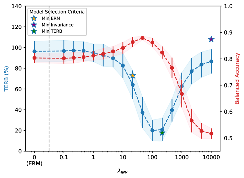
(a) Experiment Sampling

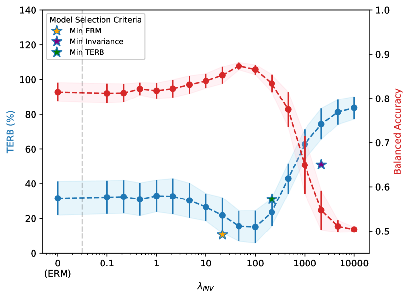
(b) Position Sampling

Figure 2: TERB and Balanced Accuracy with standard deviation over 20 different seeds varying the invariance weight $\lambda_{\text{INV}}$ of vRex (Krueger et al., 2021) on ISTAnt dataset (Cadei et al., 2024). With stars, the TERB of the model is selected by different model selection criteria on a small but heterogeneous validation set.

5.2 Synthetic Ablation with “Ninterventions”

This subsection presents identifiability results under controversial (non-causal) conditions using simulated data. We consider the synthetic setup with full control over the latent space and the data-generating process. We consider a simple graph of three causal variables as $\mathbf{z}_{1}\rightarrow\mathbf{z}_{2}\rightarrow\mathbf{z}_{3}$. The corresponding joint density has the form of

$$p_{\mathbf{z}}(z_{1},z_{2},z_{3})=p(z_{3}~{}|~{}z_{2})p(z_{2}~{}|~{}z_{1})p(z_{1}),$$ (5.1)

The goal of this experiment is to demonstrate that existing methods for interventional CRL rely primarily on distributional invariance, regardless of whether this invariance arises from a well-defined intervention or some other arbitrary transformation. To illustrate this, we introduce the concept of a “nintervention," which has a similar distributional effect to a regular intervention, maintaining certain conditionals invariant while altering others, but without a causal interpretation.

Definition 5.1 (Ninterrventions).

We define a “nintervention” on a causal conditional as the process of changing its distribution but cutting all incoming and outgoing edges. Child nodes condition on the old, pre-intervention, random variable. Formally, we consider the latent SCM as defined in Defn. 2.1, an nintervention on a node $j\in[N]$ is gives rise to the following conditional factorization

$$\tilde{p}_{\mathbf{z}}(z)=\tilde{p}(z_{j})\prod_{i\in[N]\setminus\{j\}}p(z_{i}~{}|~{}{z}_{\text{pa}({i})}^{\text{old}})$$

Note that the marginal distribution of all non-nintervened nodes $P_{\mathbf{z}_{[N]\setminus j}}$ remain invariant after nintervention. In previous example, we perform a nintervention by replacing the conditional density $p(z_{2}~{}|~{}z_{1})$ using a sufficiently different marginal distribution $p(\tilde{z}_{2})$ that satisfies Defn. 2.3 (ii), which gives rise to the following new factorization:

$$\tilde{p}_{\mathbf{z}}(z_{1},z_{2},z_{3})=p(z_{3}~{}|~{}z_{2}^{\text{old}})\tilde{p}(z_{2})p(z_{1}).$$ (5.2)

Note that $\mathbf{z}_{3}$ conditions on the random variable $\mathbf{z}_{2}$ before nintervention, whose realization is denoted as $z_{2}^{\text{old}}$. Differing from a intervention from the causal sense, we cut not only the incoming link of $\mathbf{z}_{2}$ but also its outgoing connection by keeping the marginal distribution of $\mathbf{z}_{3}$ the same. Clearly, this is a non-sensical intervention from the causal perspective because we eliminates the causal effect from $\mathbf{z}_{2}$ to its descendants.

Experimental setting. As a proof of concept, we choose a linear Gaussian additive noise model and a nonlinear mixing function implemented as a 3-layer invertible MLP with Leaky-ReLU activation. We average the results over three independently sampled ninterventional densities $\tilde{p}(z_{2})$ while guaranteeing all ninterventional distributions satisfy Defn. 2.3 (ii). We remark that the marginal distribution of both $\mathbf{z}_{1},\mathbf{z}_{3}$ remains the same after a nintervention. Hence, we expect $\mathbf{z}_{1},\mathbf{z}_{3}$ to be block-identified (Defn. 3.1) according to Thm. 3.1.

In practice, we enforce the marginal invariance constraint (Constraint 3.1) by minimizing the MMD loss, as implemented by the interventional CRL works (Zhang et al., 2024a; Ahuja et al., 2024) and train an auto-encoder for a sufficient representation (Constraint 3.2). Further details are included in LABEL:app:experiments.

Results. To validate block-identifiability, we perform Kernel-Ridge Regression between the estimated block $[\hat{\mathbf{z}}_{1},\hat{\mathbf{z}}_{3}]$ and the ground truth latents $\mathbf{z}_{1},\mathbf{z}_{2},\mathbf{z}_{3}$ respectively. The results indicate that both $\mathbf{z}_{1},\mathbf{z}_{3}$ are block-identified, showing a high $R^{2}$ score of $0.863\pm 0.031$ and $0.872\pm 0.035$, respectively. By contrast, the latent variable $\mathbf{z}_{2}$ is not identified, evidenced by a low $R^{2}$ of $0.065\pm 0.017$.

Discussion. By showing the block-identifiability results of marginal invariant latent variables $\mathbf{z}_{1},\mathbf{z}_{3}$ under nintervention, we successfully validate Thm. 3.1, demystifying the spurious link between latent variable identification and causal interventions. Throughout the experiment, we realize that a sufficiently different ninterventional distribution (Defn. 2.3 (ii)) is the key to validate the identification theory properly and to observe the expected outcome, as elaborated in LABEL:app:ass_justification.

6 Conclusions

In this paper, we take a closer look at the wide range of causal representation learning methods. Interestingly, we find that the differences between them may often be more related to “semantics" than to fundamental methodological distinctions. We identified two components involved in identifiability results: preserving information of the data and a set of known invariances. Our results have two immediate implications. First, they provide new insights into the “causal representation learning problem," particularly clarifying the role of causal assumptions. We have shown that while learning the graph requires traditional causal assumptions such as additive noise models or access to interventions, identifying the causal variables may not. This is an important result, as access to causal variables is standalone useful for downstream tasks, e.g., for training robust downstream predictors or even extracting pre-treatment covariates for treatment effect estimation (Yao et al., 2024), even without knowledge of the full causal graph. Second, we have exemplified how causal representation can lead to successful applications in practice. We moved the goal post from a characterization of specific assumptions that lead to identifiability, which often do not align with real-world data, to a general recipe that allow practitioners to specify known invariances in their problem and learn representations that align with them. In the domain generalization literature, it has been widely observed that invariant training methods often do not consistently outperform empirical risk minimization (ERM). In our experiments, instead, we have demonstrated that the specific invariance enforced by vREX (Krueger et al., 2021) entails good performance in our causal downstream task (§ 5.1). Our paper leaves out certain settings concerning identifiability that may be interesting for future work, such as discrete variables and finite samples guarantees.

One question the reader may ask, then, is “so what is exactly causal in causal representation learning?”. We have shown that the identifiability results in typical causal representation learning are primarily based on invariance assumptions, which do not necessarily pertain to causality. We hope this insight will broaden the applicability of these methods. At the same time, we used causality as a language describing the “parameterization” of the system in terms of latent causal variables with associated known symmetries. Defining the symmetries at the level of these causal variables gives the identified representation a causal meaning, important when incorporating a graph discovery step or some other causal downstream task like treatment effect estimation. Ultimately, our representations and latent causal models can be “true” in the sense of (Peters et al., 2014) when they allow us to predict “causal effects that one observes in practice”. Overall, our view also aligns with “phenomenological” accounts of causality (Janzing and Mejia, 2024), that define causal variables from a set of elementary interventions. In our setting too, the identified latent variables or blocks thereof are directly defined by the invariances at hand. From the methodological perspective, all is needed to learn causal variables is for the symmetries defined over the causal latent variables to entail some statistical footprint across pockets of data. If variables are available, learning the graph has a rich literature (Peters et al., 2017), with assumptions that are often compatible with learning the variables themselves. Our general characterization of the variable learning problem opens new frontiers for research in representation learning:

6.1 Representational Alignment and Platonic Representation

Several works (Li et al. (2015); Moschella et al. (2022); Kornblith et al. (2019); Huh et al. (2024)) have highlighted the emergence of similar representations in neural models trained independently. In Huh et al. (2024) is hypothesized that neural networks, trained with different objectives on various data and modalities, are converging toward a shared statistical model of reality within their representation spaces. To support this hypothesis, they measure the alignment of representations proposing to use a mutual nearest-neighbor metric, which measures the mean intersection of the k-nearest neighbor sets induced by two kernels defined on the two spaces, normalized by k. This metric can be an instance to the distance function in our formulation in Thm. 3.1. Despite not being optimized directly, several models in multiple settings (different objectives, data and modalities) seem to be aligned, hinting at the fact that their individual training objectives may be respecting some unknwon symmetries. A precise formalization of the latent causal model and identifiability in the context of foundational models remains open and will be objective for future research.

6.2 Environment Discovery

Domain generalization methods generalize to distributions potentially far away from the training, distribution, via learning representations invariant across distinct environments. However this can be costly as it requires to have label information informing on the partition of the data into environments. Automatic environment discovery (Creager et al. (2021); Arefin et al. (2024); Pezeshki et al. (2024)) attempts to solve this problem by learning to recover the environment partition. This is an interesting new frontier for causal representation learning, discovering data symmetries as opposed to only enforcing them. For example, this would correspond to having access to multiple interventional distributions but without knowing which samples belong to the same interventional or observational distribution. Discovering that a data set is a mixture of distributions, each being a different intervention on the same causal model, could help increase applicability of causal representations to large obeservational data sets. We expect this to be particularly relevant to downstream tasks were biases to certain experimental settings are undesirable, as in our case study on treatment effect estimation from high-dimensional recordings of a randomized controlled trial.

6.3 Connection with Geometric Deep Learning

Geometric deep learning (GDL) (Bronstein et al. (2017, 2021)) is a well estabilished learning paradigm which involves encoding a geometric understanding of data as an inductive bias in deep learning models, in order to obtain more robust models and improve performance. One fundamental direction for these priors is to encode symmetries and invariances to different types of transformations of the input data, e.g. rotations or group actions (Cohen and Welling (2016); Cohen et al. (2018)), in representational space. Our work can be fundamentally related with this direction, with the difference that we don’t aim to model explicitly the transformations of the input space, but the invariances defined at the latent level. While an initial connection has been developed for disentanglement Fumero et al. (2021); Higgins et al. (2018), a precise connection between GDL and causal representation learning remains a open direction. We expect this to benefit the two communities in both directions: (i) by injecting geometric priors in order to craft better CRL algorithms and (ii) by incorporating causality into successful GDL frameworks, which have been fundamentally advancing challenging real-world problems, such as protein folding (Jumper et al. (2021)).

Appendix

Appendix A Notation and Terminology

References

- Schölkopf et al. (2021) Bernhard Schölkopf, Francesco Locatello, Stefan Bauer, Nan Rosemary Ke, Nal Kalchbrenner, Anirudh Goyal, and Yoshua Bengio. Toward causal representation learning. Proceedings of the IEEE, 109(5):612–634, 2021.
- Vigário et al. (1997) Ricardo Vigário, Veikko Jousmäki, Matti Hämäläinen, Riitta Hari, and Erkki Oja. Independent component analysis for identification of artifacts in magnetoencephalographic recordings. Advances in neural information processing systems, 10, 1997.
- Brown et al. (2001) Glen D Brown, Satoshi Yamada, and Terrence J Sejnowski. Independent component analysis at the neural cocktail party. Trends in neurosciences, 24(1):54–63, 2001.
- Ristaniemi (1999) Tapani Ristaniemi. On the performance of blind source separation in cdma downlink. In Proceedings of the International Workshop on Independent Component Analysis and Signal Separation (ICA’99), pages 437–441, 1999.
- Donoho (2006) David L Donoho. Compressed sensing. IEEE Transactions on information theory, 52(4):1289–1306, 2006.
- Angrist and Pischke (2009) Joshua D Angrist and Jörn-Steffen Pischke. Mostly harmless econometrics: An empiricist’s companion. Princeton university press, 2009.
- Antonakis and Lalive (2011) J Antonakis and R Lalive. Counterfactuals and causal inference: Methods and principles for social research. Structural Equation Modeling, 18(1):152–159, 2011.
- Ahuja et al. (2022a) Kartik Ahuja, Ethan Caballero, Dinghuai Zhang, Jean-Christophe Gagnon-Audet, Yoshua Bengio, Ioannis Mitliagkas, and Irina Rish. Invariance principle meets information bottleneck for out-of-distribution generalization, 2022a.
- Bareinboim and Pearl (2016) Elias Bareinboim and Judea Pearl. Causal inference and the data-fusion problem. Proceedings of the National Academy of Sciences, 113(27):7345–7352, 2016.
- Rojas-Carulla et al. (2018) Mateo Rojas-Carulla, Bernhard Schölkopf, Richard Turner, and Jonas Peters. Invariant models for causal transfer learning. Journal of Machine Learning Research, 19(36):1–34, 2018.
- Fumero et al. (2024) Marco Fumero, Florian Wenzel, Luca Zancato, Alessandro Achille, Emanuele Rodolà, Stefano Soatto, Bernhard Schölkopf, and Francesco Locatello. Leveraging sparse and shared feature activations for disentangled representation learning. Advances in Neural Information Processing Systems, 36, 2024.
- Seitzer et al. (2021) Maximilian Seitzer, Bernhard Schölkopf, and Georg Martius. Causal influence detection for improving efficiency in reinforcement learning. Advances in Neural Information Processing Systems, 34:22905–22918, 2021.
- Urpí et al. (2024) Núria Armengol Urpí, Marco Bagatella, Marin Vlastelica, and Georg Martius. Causal action influence aware counterfactual data augmentation. Forty-first International Conference on Machine Learning, 2024.
- von Kügelgen et al. (2024) Julius von Kügelgen, Michel Besserve, Liang Wendong, Luigi Gresele, Armin Kekić, Elias Bareinboim, David Blei, and Bernhard Schölkopf. Nonparametric identifiability of causal representations from unknown interventions. Advances in Neural Information Processing Systems, 36, 2024.
- Ahuja et al. (2023) Kartik Ahuja, Divyat Mahajan, Yixin Wang, and Yoshua Bengio. Interventional causal representation learning. In International Conference on Machine Learning, pages 372–407. PMLR, 2023.
- Brehmer et al. (2022) Johann Brehmer, Pim De Haan, Phillip Lippe, and Taco S Cohen. Weakly supervised causal representation learning. Advances in Neural Information Processing Systems, 35:38319–38331, 2022.
- Buchholz et al. (2023) Simon Buchholz, Goutham Rajendran, Elan Rosenfeld, Bryon Aragam, Bernhard Schölkopf, and Pradeep Ravikumar. Learning linear causal representations from interventions under general nonlinear mixing. arXiv preprint arXiv:2306.02235, 2023.
- Zhang et al. (2024a) Jiaqi Zhang, Kristjan Greenewald, Chandler Squires, Akash Srivastava, Karthikeyan Shanmugam, and Caroline Uhler. Identifiability guarantees for causal disentanglement from soft interventions. Advances in Neural Information Processing Systems, 36, 2024a.
- Varici et al. (2024a) Burak Varici, Emre Acartürk, Karthikeyan Shanmugam, and Ali Tajer. General identifiability and achievability for causal representation learning. In International Conference on Artificial Intelligence and Statistics, pages 2314–2322. PMLR, 2024a.
- Lachapelle et al. (2022) Sébastien Lachapelle, Rodriguez Lopez, Pau, Yash Sharma, Katie E. Everett, Rémi Le Priol, Alexandre Lacoste, and Simon Lacoste-Julien. Disentanglement via mechanism sparsity regularization: A new principle for nonlinear ICA. In First Conference on Causal Learning and Reasoning, 2022.
- Lippe et al. (2022a) Phillip Lippe, Sara Magliacane, Sindy Löwe, Yuki M Asano, Taco Cohen, and Efstratios Gavves. Causal representation learning for instantaneous and temporal effects in interactive systems. In The Eleventh International Conference on Learning Representations, 2022a.
- Lippe et al. (2022b) Phillip Lippe, Sara Magliacane, Sindy Löwe, Yuki M Asano, Taco Cohen, and Stratis Gavves. Citris: Causal identifiability from temporal intervened sequences. In International Conference on Machine Learning, pages 13557–13603. PMLR, 2022b.
- Lippe et al. (2023) Phillip Lippe, Sara Magliacane, Sindy Löwe, Yuki M Asano, Taco Cohen, and Efstratios Gavves. Biscuit: Causal representation learning from binary interactions. arXiv preprint arXiv:2306.09643, 2023.
- Sagawa et al. (2019) Shiori Sagawa, Pang Wei Koh, Tatsunori B Hashimoto, and Percy Liang. Distributionally robust neural networks for group shifts: On the importance of regularization for worst-case generalization. arXiv preprint arXiv:1911.08731, 2019.
- Krueger et al. (2021) David Krueger, Ethan Caballero, Joern-Henrik Jacobsen, Amy Zhang, Jonathan Binas, Dinghuai Zhang, Remi Le Priol, and Aaron Courville. Out-of-distribution generalization via risk extrapolation (rex). In International conference on machine learning, pages 5815–5826. PMLR, 2021.
- Lachapelle et al. (2023) Sébastien Lachapelle, Tristan Deleu, Divyat Mahajan, Ioannis Mitliagkas, Yoshua Bengio, Simon Lacoste-Julien, and Quentin Bertrand. Synergies between disentanglement and sparsity: Generalization and identifiability in multi-task learning. In International Conference on Machine Learning, pages 18171–18206. PMLR, 2023.
- Cadei et al. (2024) Riccardo Cadei, Lukas Lindorfer, Sylvia Cremer, Cordelia Schmid, and Francesco Locatello. Smoke and mirrors in causal downstream tasks. arXiv preprint arXiv:2405.17151, 2024.
- Arjovsky et al. (2020) Martin Arjovsky, Léon Bottou, Ishaan Gulrajani, and David Lopez-Paz. Invariant risk minimization, 2020.
- Cohen and Welling (2016) Taco Cohen and Max Welling. Group equivariant convolutional networks. In International conference on machine learning, pages 2990–2999. PMLR, 2016.
- Bronstein et al. (2017) Michael M Bronstein, Joan Bruna, Yann LeCun, Arthur Szlam, and Pierre Vandergheynst. Geometric deep learning: going beyond euclidean data. IEEE Signal Processing Magazine, 34(4):18–42, 2017.
- Bronstein et al. (2021) Michael M Bronstein, Joan Bruna, Taco Cohen, and P Velickovic. Geometric deep learning: Grids, groups, graphs, geodesics, and gauges. arxiv 2021. arXiv preprint arXiv:2104.13478, 2021.
- von Kügelgen et al. (2021) Julius von Kügelgen, Yash Sharma, Luigi Gresele, Wieland Brendel, Bernhard Schölkopf, Michel Besserve, and Francesco Locatello. Self-supervised learning with data augmentations provably isolates content from style. Advances in neural information processing systems, 34:16451–16467, 2021.
- Yao et al. (2023) Dingling Yao, Danru Xu, Sebastien Lachapelle, Sara Magliacane, Perouz Taslakian, Georg Martius, Julius von Kügelgen, and Francesco Locatello. Multi-view causal representation learning with partial observability. In The Twelfth International Conference on Learning Representations, 2023.
- Varici et al. (2023) Burak Varici, Emre Acarturk, Karthikeyan Shanmugam, Abhishek Kumar, and Ali Tajer. Score-based causal representation learning with interventions. arXiv preprint arXiv:2301.08230, 2023.
- Varici et al. (2024b) Burak Varici, Emre Acartürk, Karthikeyan Shanmugam, and Ali Tajer. Linear causal representation learning from unknown multi-node interventions. arXiv preprint arXiv:2406.05937, 2024b.
- Liang et al. (2023) Wendong Liang, Armin Kekić, Julius von Kügelgen, Simon Buchholz, Michel Besserve, Luigi Gresele, and Bernhard Schölkopf. Causal component analysis. arXiv preprint arXiv:2305.17225, 2023.
- Daunhawer et al. (2023) Imant Daunhawer, Alice Bizeul, Emanuele Palumbo, Alexander Marx, and Julia E Vogt. Identifiability results for multimodal contrastive learning. In The Eleventh International Conference on Learning Representations, 2023.
- Locatello et al. (2020) Francesco Locatello, Ben Poole, Gunnar Raetsch, Bernhard Schölkopf, Olivier Bachem, and Michael Tschannen. Weakly-supervised disentanglement without compromises. In Hal Daumé III and Aarti Singh, editors, Proceedings of the 37th International Conference on Machine Learning, volume 119 of Proceedings of Machine Learning Research, pages 6348–6359. PMLR, 13–18 Jul 2020.
- Ahuja et al. (2022b) Kartik Ahuja, Jason S Hartford, and Yoshua Bengio. Weakly supervised representation learning with sparse perturbations. Advances in Neural Information Processing Systems, 35:15516–15528, 2022b.
- Zimmermann et al. (2021) Roland S Zimmermann, Yash Sharma, Steffen Schneider, Matthias Bethge, and Wieland Brendel. Contrastive learning inverts the data generating process. In International Conference on Machine Learning, pages 12979–12990. PMLR, 2021.
- Squires et al. (2023) Chandler Squires, Anna Seigal, Salil S. Bhate, and Caroline Uhler. Linear causal disentanglement via interventions. In International Conference on Machine Learning, volume 202, pages 32540–32560. PMLR, 2023.
- Lachapelle et al. (2024) Sébastien Lachapelle, Pau Rodríguez López, Yash Sharma, Katie Everett, Rémi Le Priol, Alexandre Lacoste, and Simon Lacoste-Julien. Nonparametric partial disentanglement via mechanism sparsity: Sparse actions, interventions and sparse temporal dependencies, 2024.
- Zheng et al. (2022) Yujia Zheng, Ignavier Ng, and Kun Zhang. On the identifiability of nonlinear ica: Sparsity and beyond. Advances in neural information processing systems, 35:16411–16422, 2022.
- Xu et al. (2024) Danru Xu, Dingling Yao, Sébastien Lachapelle, Perouz Taslakian, Julius von Kügelgen, Francesco Locatello, and Sara Magliacane. A sparsity principle for partially observable causal representation learning. Forty-first International Conference on Machine Learning, 2024.
- Ahuja et al. (2024) Kartik Ahuja, Amin Mansouri, and Yixin Wang. Multi-domain causal representation learning via weak distributional invariances. In International Conference on Artificial Intelligence and Statistics, pages 865–873. PMLR, 2024.
- Locatello et al. (2019) Francesco Locatello, Stefan Bauer, Mario Lucic, Gunnar Raetsch, Sylvain Gelly, Bernhard Schölkopf, and Olivier Bachem. Challenging common assumptions in the unsupervised learning of disentangled representations. In international conference on machine learning, pages 4114–4124. PMLR, 2019.
- Pearl (2009) Judea Pearl. Causality. Cambridge university press, 2009.
- Hoyer et al. (2008) Patrik Hoyer, Dominik Janzing, Joris M Mooij, Jonas Peters, and Bernhard Schölkopf. Nonlinear causal discovery with additive noise models. Advances in neural information processing systems, 21, 2008.
- Zhang and Hyvärinen (2010) Kun Zhang and Aapo Hyvärinen. Distinguishing causes from effects using nonlinear acyclic causal models. In Causality: Objectives and Assessment, pages 157–164. PMLR, 2010.
- Zhang and Hyvärinen (2009) K Zhang and A Hyvärinen. On the identifiability of the post-nonlinear causal model. In 25th Conference on Uncertainty in Artificial Intelligence (UAI 2009), pages 647–655. AUAI Press, 2009.
- Rubenstein et al. (2017) P Rubenstein, S Weichwald, S Bongers, J Mooij, D Janzing, M Grosse-Wentrup, and B Schölkopf. Causal consistency of structural equation models. In 33rd Conference on Uncertainty in Artificial Intelligence (UAI 2017), pages 808–817. Curran Associates, Inc., 2017.
- Beckers and Halpern (2019) Sander Beckers and Joseph Y Halpern. Abstracting causal models. In Proceedings of the aaai conference on artificial intelligence, volume 33, pages 2678–2685, 2019.
- Rubin (2005) Donald B Rubin. Causal inference using potential outcomes: Design, modeling, decisions. Journal of the American Statistical Association, 100(469):322–331, 2005.
- Liu et al. (2023) Yuejiang Liu, Alexandre Alahi, Chris Russell, Max Horn, Dominik Zietlow, Bernhard Schölkopf, and Francesco Locatello. Causal triplet: An open challenge for intervention-centric causal representation learning. In Conference on Causal Learning and Reasoning, pages 553–573. PMLR, 2023.
- Zhang et al. (2024b) Kun Zhang, Shaoan Xie, Ignavier Ng, and Yujia Zheng. Causal representation learning from multiple distributions: A general setting. Internatinal Conference on Machine Learning, 2024b.
- Yao et al. (2022a) Weiran Yao, Guangyi Chen, and Kun Zhang. Temporally disentangled representation learning. Advances in Neural Information Processing Systems, 35:26492–26503, 2022a.
- Yao et al. (2022b) Weiran Yao, Yuewen Sun, Alex Ho, Changyin Sun, and Kun Zhang. Learning temporally causal latent processes from general temporal data, 2022b.
- Li et al. (2024a) Zijian Li, Ruichu Cai, Zhenhui Yang, Haiqin Huang, Guangyi Chen, Yifan Shen, Zhengming Chen, Xiangchen Song, Zhifeng Hao, and Kun Zhang. When and how: Learning identifiable latent states for nonstationary time series forecasting. arXiv preprint arXiv:2402.12767, 2024a.
- Li et al. (2024b) Zijian Li, Yifan Shen, Kaitao Zheng, Ruichu Cai, Xiangchen Song, Mingming Gong, Zhifeng Hao, Zhengmao Zhu, Guangyi Chen, and Kun Zhang. On the identification of temporally causal representation with instantaneous dependence. arXiv preprint arXiv:2405.15325, 2024b.
- Dean and Kanazawa (1989) Thomas Dean and Keiji Kanazawa. A model for reasoning about persistance and causation. In Computational Intelligence, page 5, 1989.
- Murphy (2002) Kevin Patrick Murphy. Dynamic bayesian networks: representation, inference and learning. University of California, Berkeley, 2002.
- Klindt et al. (2021) David A Klindt, Lukas Schott, Yash Sharma, Ivan Ustyuzhaninov, Wieland Brendel, Matthias Bethge, and Dylan Paiton. Towards nonlinear disentanglement in natural data with temporal sparse coding. In International Conference on Learning Representations, 2021.
- Khemakhem et al. (2020) Ilyes Khemakhem, Ricardo Monti, Diederik Kingma, and Aapo Hyvarinen. Ice-beem: Identifiable conditional energy-based deep models based on nonlinear ica. Advances in Neural Information Processing Systems, 33:12768–12778, 2020.
- Kingma and Welling (2013) Diederik P Kingma and Max Welling. Auto-encoding variational bayes. arXiv preprint arXiv:1312.6114, 2013.
- Rezende and Mohamed (2016) Danilo Jimenez Rezende and Shakir Mohamed. Variational inference with normalizing flows, 2016.
- Caruana (1997) Rich Caruana. Multitask learning. Machine learning, 28:41–75, 1997.
- Zhang and Yang (2018) Yu Zhang and Qiang Yang. An overview of multi-task learning. National Science Review, 5(1):30–43, 2018.
- Zhu et al. (2022) Jinguo Zhu, Xizhou Zhu, Wenhai Wang, Xiaohua Wang, Hongsheng Li, Xiaogang Wang, and Jifeng Dai. Uni-perceiver-moe: Learning sparse generalist models with conditional moes. Advances in Neural Information Processing Systems, 35:2664–2678, 2022.
- Bai et al. (2022) Jinze Bai, Rui Men, Hao Yang, Xuancheng Ren, Kai Dang, Yichang Zhang, Xiaohuan Zhou, Peng Wang, Sinan Tan, An Yang, et al. Ofasys: A multi-modal multi-task learning system for building generalist models. arXiv preprint arXiv:2212.04408, 2022.
- Zhang et al. (2017) Hongyi Zhang, Moustapha Cisse, Yann N Dauphin, and David Lopez-Paz. mixup: Beyond empirical risk minimization. arXiv preprint arXiv:1710.09412, 2017.
- Ganin et al. (2016) Yaroslav Ganin, Evgeniya Ustinova, Hana Ajakan, Pascal Germain, Hugo Larochelle, François Laviolette, Mario March, and Victor Lempitsky. Domain-adversarial training of neural networks. Journal of machine learning research, 17(59):1–35, 2016.
- Fang et al. (2013) Chen Fang, Ye Xu, and Daniel N Rockmore. Unbiased metric learning: On the utilization of multiple datasets and web images for softening bias. In Proceedings of the IEEE International Conference on Computer Vision, pages 1657–1664, 2013.
- Li et al. (2017) Da Li, Yongxin Yang, Yi-Zhe Song, and Timothy M Hospedales. Deeper, broader and artier domain generalization. In Proceedings of the IEEE international conference on computer vision, pages 5542–5550, 2017.
- Venkateswara et al. (2017) Hemanth Venkateswara, Jose Eusebio, Shayok Chakraborty, and Sethuraman Panchanathan. Deep hashing network for unsupervised domain adaptation. In Proceedings of the IEEE conference on computer vision and pattern recognition, pages 5018–5027, 2017.
- Beery et al. (2018) Sara Beery, Grant Van Horn, and Pietro Perona. Recognition in terra incognita. In Proceedings of the European conference on computer vision (ECCV), pages 456–473, 2018.
- Peng et al. (2019) Xingchao Peng, Qinxun Bai, Xide Xia, Zijun Huang, Kate Saenko, and Bo Wang. Moment matching for multi-source domain adaptation. In Proceedings of the IEEE/CVF international conference on computer vision, pages 1406–1415, 2019.
- Blanchard et al. (2011) Gilles Blanchard, Gyemin Lee, and Clayton Scott. Generalizing from several related classification tasks to a new unlabeled sample. Advances in neural information processing systems, 24, 2011.
- Zhou et al. (2022) Kaiyang Zhou, Ziwei Liu, Yu Qiao, Tao Xiang, and Chen Change Loy. Domain generalization: A survey. IEEE Transactions on Pattern Analysis and Machine Intelligence, 45(4):4396–4415, 2022.
- Robins et al. (2000) James M Robins, Miguel Angel Hernan, and Babette Brumback. Marginal structural models and causal inference in epidemiology. Epidemiology, 11(5):550–560, 2000.
- Samet et al. (2000) Jonathan M Samet, Francesca Dominici, Frank C Curriero, Ivan Coursac, and Scott L Zeger. Fine particulate air pollution and mortality in 20 us cities, 1987–1994. New England journal of medicine, 343(24):1742–1749, 2000.
- Van Nes et al. (2015) Egbert H Van Nes, Marten Scheffer, Victor Brovkin, Timothy M Lenton, Hao Ye, Ethan Deyle, and George Sugihara. Causal feedbacks in climate change. Nature Climate Change, 5(5):445–448, 2015.
- Runge (2023) Jakob Runge. Modern causal inference approaches to investigate biodiversity-ecosystem functioning relationships. nature communications, 14(1):1917, 2023.
- Gulrajani and Lopez-Paz (2020) Ishaan Gulrajani and David Lopez-Paz. In search of lost domain generalization. arXiv preprint arXiv:2007.01434, 2020.
- Yao et al. (2024) Dingling Yao, Caroline Muller, and Francesco Locatello. Marrying causal representation learning with dynamical systems for science. arXiv preprint arXiv:2405.13888, 2024.
- Peters et al. (2014) Jonas Peters, Joris M Mooij, Dominik Janzing, and Bernhard Schölkopf. Causal discovery with continuous additive noise models. Journal of Machine Learning Research, 2014.
- Janzing and Mejia (2024) Dominik Janzing and Sergio Hernan Garrido Mejia. A phenomenological account for causality in terms of elementary actions. Journal of Causal Inference, 12(1):20220076, 2024.
- Peters et al. (2017) Jonas Peters, Dominik Janzing, and Bernhard Schlkopf. Elements of Causal Inference: Foundations and Learning Algorithms. The MIT Press, 2017. ISBN 0262037319.
- Li et al. (2015) Yixuan Li, Jason Yosinski, Jeff Clune, Hod Lipson, and John Hopcroft. Convergent learning: Do different neural networks learn the same representations? arXiv preprint arXiv:1511.07543, 2015.
- Moschella et al. (2022) Luca Moschella, Valentino Maiorca, Marco Fumero, Antonio Norelli, Francesco Locatello, and Emanuele Rodolà. Relative representations enable zero-shot latent space communication. arXiv preprint arXiv:2209.15430, 2022.
- Kornblith et al. (2019) Simon Kornblith, Mohammad Norouzi, Honglak Lee, and Geoffrey Hinton. Similarity of neural network representations revisited. In International conference on machine learning, pages 3519–3529. PMLR, 2019.
- Huh et al. (2024) Minyoung Huh, Brian Cheung, Tongzhou Wang, and Phillip Isola. The platonic representation hypothesis. arXiv preprint arXiv:2405.07987, 2024.
- Creager et al. (2021) Elliot Creager, Joern-Henrik Jacobsen, and Richard Zemel. Environment inference for invariant learning. In Marina Meila and Tong Zhang, editors, Proceedings of the 38th International Conference on Machine Learning, volume 139 of Proceedings of Machine Learning Research, pages 2189–2200. PMLR, 18–24 Jul 2021.
- Arefin et al. (2024) Md Rifat Arefin, Yan Zhang, Aristide Baratin, Francesco Locatello, Irina Rish, Dianbo Liu, and Kenji Kawaguchi. Unsupervised concept discovery mitigates spurious correlations. In Forty-first International Conference on Machine Learning, 2024.
- Pezeshki et al. (2024) Mohammad Pezeshki, Diane Bouchacourt, Mark Ibrahim, Nicolas Ballas, Pascal Vincent, and David Lopez-Paz. Discovering environments with xrm. In Forty-first International Conference on Machine Learning, 2024.
- Cohen et al. (2018) Taco S Cohen, Mario Geiger, Jonas Köhler, and Max Welling. Spherical cnns. arXiv preprint arXiv:1801.10130, 2018.
- Fumero et al. (2021) Marco Fumero, Luca Cosmo, Simone Melzi, and Emanuele Rodolà. Learning disentangled representations via product manifold projection. In International conference on machine learning, pages 3530–3540. PMLR, 2021.
- Higgins et al. (2018) Irina Higgins, David Amos, David Pfau, Sebastien Racaniere, Loic Matthey, Danilo Rezende, and Alexander Lerchner. Towards a definition of disentangled representations. arXiv preprint arXiv:1812.02230, 2018.
- Jumper et al. (2021) John Jumper, Richard Evans, Alexander Pritzel, Tim Green, Michael Figurnov, Olaf Ronneberger, Kathryn Tunyasuvunakool, Russ Bates, Augustin Žídek, Anna Potapenko, et al. Highly accurate protein structure prediction with alphafold. nature, 596(7873):583–589, 2021.
- Kivva et al. (2022) Bohdan Kivva, Goutham Rajendran, Pradeep Ravikumar, and Bryon Aragam. Identifiability of deep generative models without auxiliary information. In S. Koyejo, S. Mohamed, A. Agarwal, D. Belgrave, K. Cho, and A. Oh, editors, Advances in Neural Information Processing Systems, volume 35, pages 15687–15701. Curran Associates, Inc., 2022.