Magnetic, Kinetic, and Transition regime: Spatially-segregated structure of compressive MHD turbulence

Abstract

Turbulence is a complex physical process that emerges in multiple areas of modern physics, and in ionized environments such as interstellar gas, the magnetic field can be dynamically important. However, the exact function of the magnetic field in the ionized gas remains unclear. We use the ${\cal M}_{\rm A}=\sqrt{E_{\rm k}/E_{B}}$ to describe the importance of the magnetic field measured to the turbulent motion, and reveal diverse ways of mutual interaction. At low ${\cal M}_{\rm A}$ (magnetic regime), the magnetic field is well-described as force-free. Despite the strong magnetic field, the motion of gas does not stay aligned with the magnetic field. At the regime of intermediate ${\cal M}_{\rm A}$ (magnetic-kinetic transition regime), the velocity field and the magnetic field exhibit the highest degree of alignment, which is likely the result of a rapid relaxation. At high ${\cal M}_{\rm A}$ (kinetic regime), both the magnetic field and the velocity field are irregular, with no alignment. We find observational counterparts to these regimes in observations of interstellar gas. The results highlight the diverse behavior of gas in MHD turbulence and guide future interpretations of the role of the magnetic field in astrophysical observations.

1 Introduction

Turbulence is a complex process that has puzzled scientists since the age of Leonardo da Vinci, and the capability of turbulence in controlling the evolution of interstellar gas has been known for decades (Mac Low & Klessen, 2004). Understanding the role of the magnetic field in compressible turbulence can be crucial for our understanding of turbulence and for interpreting astrophysical observations. Turbulence is a complex, multi-scale process Frisch (1995) best described using scaling relations Kolmogorov (1941). Past studies of compressible magnetohydrodynamics (MHD) turbulence have followed this tradition where describing the statistic properties of the region has become a priority Burkhart et al. (2020). Others have astrophysical applications in mind and have focused on the global quantities extracted from the simulation box (Padoan & Nordlund, 2011).

The alignment between vector quantities such as the magnetic field $\vec{B}$, the velocity $\vec{v}$, and the current $J$ offers insight into the behavior of the magnetized fluids. In astrophysical research, the alignment between $\vec{B}$ and $\vec{v}$ is assumed to be an indicator of the magnetic field’s ability to affect the motion of the gas. The alignment between $\vec{B}$ and $\vec{v}$ in the strongly magnetized regime is a fact often taken for granted, and this picture is the foundation for understanding phenomena such as wind from disk-star systems Pudritz et al. (2007), where the picture of beads on a wire have been widely accepted. In this picture, field lines of a magnetic field behave like rigid wires, which guide the motion of the gas. However, it is unclear to what extent can we trust this picture. On the other hand, Matthaeus et al. (2008) have shown that the rapid alignment between $\vec{v}$ and $\vec{B}$ is the result of a rapid relaxation process, where the magnetic field does not need to dominant.

The alignment between $\vec{J}$ and $\vec{B}$ is also critical. In magnetized fluids, an interesting phenomenon is the emergence of force-free fields, where the magnetic pressure much exceeds the plasma pressure, such that the Lorentz force must vanish to ensure a global balance. This force-free field is thus a direct indication of the dominance of the magnetic energy over other energetic terms. We note that the Lorentz for $\vec{F_{l}}$ is proportional to $\vec{J}\times\vec{B}$, and vanishes when $\vec{J}$ is parallel to $\vec{B}$. The alignment between $\vec{J}$ and $\vec{B}$ is thus a clear indication of the force-free field.

We study the alignment between $\vec{B}$, $\vec{v}$ and $\vec{J}$ at regions of different degrees of magnetization. To quantify the importance of the magnetic field, we use the Alfven Mach number ${\cal M}_{\rm A}=\sqrt{E_{\rm k}/E_{B}}$, where $E_{\rm k}$ is the kinetic energy density and $E_{B}$ is the magnetic energy density. We study the importance of the magnetic field under different conditions as characterized by ${\cal M}_{\rm A}$. By analyzing the alignment between the magnetic field $\vec{B}$, velocity $\vec{v}$ and current $\vec{J}$, we reveal different behaviors of the system under different ${\cal M}_{\rm A}$.

2 Data and method

We use numerical simulations of MHD equations performed using the Enzo code (Collins et al., 2010; Burkhart et al., 2015) with the constrained transport turned on. The simulation conducted in this study analyzed the impact of self-gravity and magnetic fields on supersonic turbulence in isothermal molecular clouds, using high-resolution simulations and adaptive mesh refinement techniques (Collins et al., 2012; Burkhart et al., 2015, 2020). The simulation we use has initial $\beta\approx E_{\rm k}/E_{\rm B}=0.2$. However, as the simulation proceeds, different subregions have different $\beta$ and ${\cal M}_{\rm A}$.

The Alfven Mach number ${\cal M}_{\rm A}$ is the indicator of magnetic field in MHD numerical simulation:

$${\cal M}_{\rm A}=\sqrt{\frac{E_{k}}{E_{B}}}=\sqrt{\frac{\rho\sigma_{v}^{2}/2}{B^{2}/8\pi}}=\sqrt{4\pi\rho}\frac{\sigma_{v}}{B},$$ (1)

which is the square root of the energy ratio between kinetic energy density $E_{\rm k}$ and magnetic energy density $E_{B}$. Based on the ${\cal M}_{\rm A}$, we divide the MHD turbulence into three regimes: magnetic regime, B-k transition, and kinetic regime, and study the relation between the magnetic field and the gas motion. From the magnetic field $\vec{B}$, the current $\vec{J}$ can be evaluated as

$$J=\frac{1}{\mu_{0}}\nabla\times\vec{B}\;,$$ (2)

and we study the alignment between the magnetic field $\vec{B}$ and the current $\vec{J}$, and the alignment between the magnetic field $\vec{B}$ and the velocity $\vec{v}$ at different ${\cal M}_{\rm A}$.

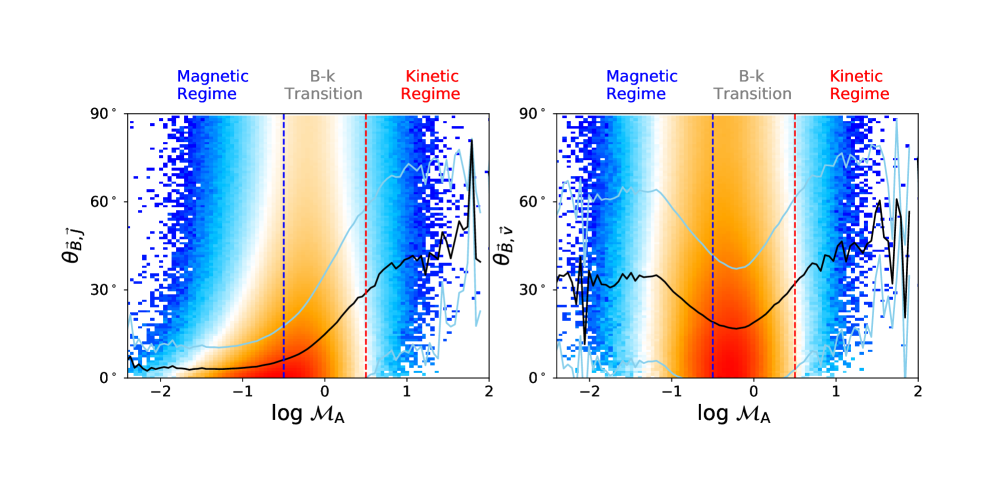
Figure 1: Distribution of ${\cal M}_{\rm A}$, $\theta_{\vec{B},\vec{J}}$, and $\theta_{\vec{B},\vec{v}}$. The left panel shows the distribution between Alfven Mach number ${\cal M}_{\rm A}$ and offset angle $\theta_{\vec{B},\vec{J}}$ between the magnetic field and current. The right panel shows the distribution between Alfven Mach number ${\cal M}_{\rm A}$ and offset angle $\theta_{\vec{B},\vec{v}}$ between the magnetic field and kinetic motion. The black line shows the main skeleton of this distribution, and the blue dash lines show its dispersion, measured at each bin. The blue and red dash lines show the ${\cal M}_{\rm A}\approx$ 0.3 and 3, respectively.

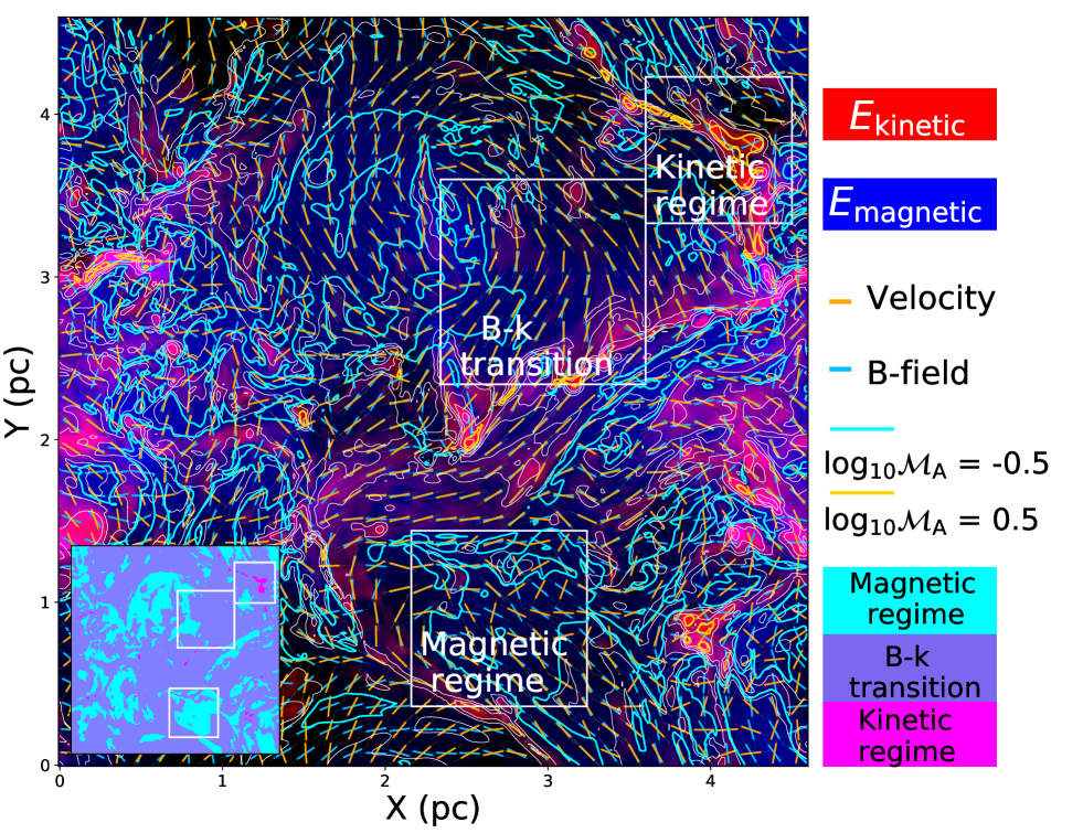
Figure 2: Alignment between magnetic field and kinetic motion. The panel shows the distribution of magnetic energy density $E_{B}$ (blue) and kinetic energy density $E_{\rm k}$ (red). Orange and blue vectors present the orientation of the magnetic field and velocity. The contours show the -0.5 (cyan) and 0. 5 (orange) of log₁₀ ${\cal M}_{\rm A}$. Locations of gas belonging to different regimes are outlined in the plot at the upper left corner.

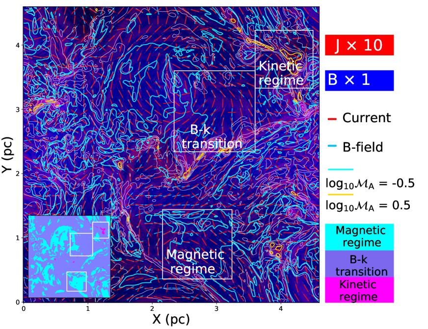
Figure 3: Alignment between magnetic field and current. The panel shows the distribution of magnetic field strength $|\vec{B}|$ (blue) and current density $|\vec{J}|$ (red). Orange and blue vectors present the orientation of the magnetic field and velocity. The contours show the log₁₀ ${\cal M}_{\rm A}$= -0.5 (cyan) and 0. 5 (orange) respectively. Locations of gas belonging to different regimes are outlined in the plot at the upper left corner.

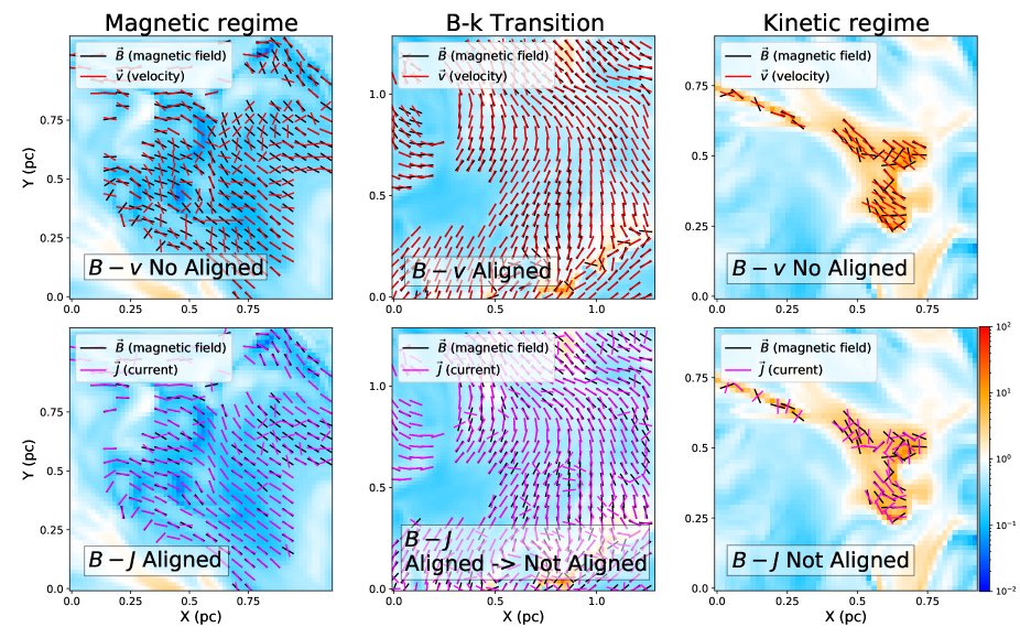
Figure 4: Alignment between magnetic field $\vec{B}$, and velocity $\vec{V}$ and current $\vec{J}$ in three different regimes. The background is the ${\cal M}_{\rm A}$ distribution in the X-Y plane. The vectors represent the orientations of the magnetic field $\vec{B}$, velocity $\vec{v}$ and current $\vec{J}$.

3 Three regimes of MHD Turbulence

Based on the Alfven Mach number ${\cal M}_{\rm A}$, we divide the simulation box into three regimes: magnetic regime (${\cal M}_{\rm A}<0.3$), B-k transition ($0.3<{\cal M}_{\rm A}<3$), and kinetic regime (${\cal M}_{\rm A}>3$), and study the alignment between the magnetic field $\vec{B}$, velocity $\vec{v}$, and current $\vec{J}$ at different ${\cal M}_{\rm A}$. The relationship between the magnetic field-velocity angle $\theta_{\vec{B}-\vec{v}}$, the magnetic field-current angle $\theta_{\vec{B}-\vec{J}}$ and the Alfven Mach number is shown in Fig. 1. When plotting these distributions, we subtract the distribution expected if the vectors are randomly oriented, and focus on the additional alignment caused by physics (see Sec. A).

With increasing ${\cal M}_{\rm A}$, the alignment between the magnetic field $\vec{B}$ and the current $\vec{J}$ changes from aligned to not aligned, and the alignment between the magnetic field $\vec{B}$ and the velocity $\vec{v}$ change from almost no alignment ($\theta_{\vec{B}-\vec{v}}\approx 30^{\circ}$), to a weak alignment ($\theta_{\vec{B}-\vec{v}}\approx 20^{\circ}$), back to no alignment ($\theta_{\vec{B}-\vec{v}}\approx 30^{\circ}$).

We note that the magnetic force is

$$\vec{f}_{\rm L}=\vec{J}\times\vec{B}\;.$$ (3)

When $\vec{J}$ is parallel to $\vec{B}$, the magnetic force vanishes, and this field configuration is called the force-free configuration. The magnetic force is activated if the angle between $\vec{J}$ and $\vec{B}$ is large.

The monotonic decrease of alignment between $\vec{B}$ and $\vec{J}$ at increasing ${\cal M}_{\rm A}$ is related to the decrease in the importance of the magnetic field, leading to the system moving away from the force-free regime. Based on the Alfven Mach number and the behavior of the system, we divide the simulation into three regimes:

• The magnetic regime (${\cal M}_{\rm A}<0.3$): the magnetic energy is far above the local kinetic energy, where the $\vec{B}$ and $\vec{v}$ do not stay aligned, yet the $\vec{B}$ and $\vec{J}$ aligned.

• The transition regime (B-k transition, $0.3<{\cal M}_{\rm A}<3$): the magnetic energy and kinetic energy have similar densities. the $\vec{B}$ and $\vec{v}$ stay aligned, and the $\vec{B}$ and $\vec{J}$ evolve from aligned to not aligned as ${\cal M}_{\rm A}$ increases.

• The kinetic regime: the kinetic energy is far above the local magnetic energy, the $\vec{B}$ and $\vec{v}$ are not aligned, and $\vec{B}$ and $\vec{J}$ are not aligned.

which are plotted in Figs. 2, 3 and 4, and are summarized in Fig. 4. Some addition slices to the simulation box can be found in Sec. B

3.1 Magnetic Regime

The first regime we discovered is the magnetic regime, where the magnetic energy is far above the local kinetic energy ($\cal{M}_{\rm A}<$ 0.3). This regime has two properties, the alignment between $\vec{B}$ and $\vec{J}$ which points to the formation of a force-free field and the lack of alignment between $\vec{B}$ and $\vec{v}$.

The strong alignment between $\vec{B}$ and $\vec{J}$ indicates that the field configuration is force-free, with other forces being dynamically unimportant. We also observe a lack of alignment between $\vec{B}$ and $\vec{v}$, which challenges the common understanding of the magnetic field being “wires” that guide the motion of the gas. In contrast, the motion of gas does not appear to stay aligned with the orientation of the magnetic field line. A strong magnetic field does not necessarily lead to motions that follow the field lines.

From astronomy observations, we identify the magnetic regime from low-density regions around some existing molecular clouds. One such example is the existence of striations located at the outer part of the Taurus molecular cloud (Heyer et al., 2016; Tritsis & Tassis, 2016).

3.2 B-k Transition

At $0.3<\cal{M}_{\rm A}$ $<3$, where the magnetic energy and the kinetic energy are similar, we find a transition regime characterized by a breakdown of the alignment between $\vec{B}$ and $J$, and a strong alignment between $\vec{B}$ and $\vec{v}$. The breakdown of the $\vec{B}$-$J$ alignment results from a decrease in the importance of the magnetic field. However, the alignment between $\vec{B}$ and $\vec{v}$ deserves further discussions.

We find the $\vec{B}$ and $\vec{v}$ only occur in the B-k transition regime, where the magnetic and kinetic energy have similar densities. This finding challenges the common understanding that the alignment between $\vec{B}$ and $\vec{v}$ indicates the dominance of the magnetic field. This alignment has been found by Matthaeus et al. (2008), which results from a “rapid and robust relaxation process in turbulent flows”. Our findings support their conclusion. However, different from the claim that “ the alignment of the velocity and magnetic field fluctuations occurs rapidly in magnetohydrodynamics for a variety of parameters”, in our case, this alignment only occurs at the transition regime with moderate $\cal{M}_{\rm A}$. In the B-k transition regime, the $vec{B}$ and $\vec{J}$ are still moderately aligned with $\theta\approx 15^{\circ}$.

From the reported values of the Alfven Mach numbers (or the mass-to-flux ratio) Pattle et al. (2023), we believe that a large number of observations of the observations are probing gas located in this transition regime. Examples include the envelope of massive star formation Orion A (Zhao et al., 2022), and other star formation regions such as Taurus, L1551 and so on (Hu et al., 2019, 2021).

3.3 Kinetic Regime

At the kinetic regime with high kinetic energy (high ${\cal M}_{\rm A}$), the $\vec{B}-\vec{v}$ not aligned, and the $\vec{B}-\vec{J}$ not aligned. The lack of this alignment is the result of the weak magnetic field.

In astronomical observations, this corresponds to dense, collapsing regions with strong turbulence, such as the Cyg N44 in Dr21 (Ching et al., 2018).

4 Conclusions

We investigate the effect of a magnetic field on supersonic turbulence. By evaluating the Alfven Mach number $\cal{M}_{\rm A}$ at different locations in a turbulence box and studying the alignment between the magnetic field $\vec{B}$, the velocity $\vec{v}$ and the current $\vec{J}$, we reveal the different behavior of the system under various conditions. These regimes include

• The magnetic regime (${\cal M}_{\rm A}<0.3$): the magnetic energy is far above the local kinetic energy, where the $\vec{B}-\vec{v}$ do not stay aligned, yet the $\vec{B}-\vec{J}$ aligned. The magnetic field is force-free.

• The transition regime (B-k transition, $0.3<{\cal M}_{\rm A}<3$): the magnetic energy and kinetic energy have similar densities. $\vec{B}$ and $\vec{v}$ are. aligned, and the $\vec{B}$ and $\vec{J}$ evolve from aligned to not aligned as ${\cal M}_{\rm A}$ increases. We also observe alignments between the magnetic field and the gas motion. However, this alignment between $\vec{B}$ and $\vec{v}$ does not imp a strong magnetic field but a rapid relaxation process in turbulent flows.

• The kinetic regime: the kinetic energy is far above the local magnetic energy, the $\vec{B}-\vec{v}$ not aligned, and the $\vec{B}-\vec{J}$ not aligned.

They are summarized in 4. Since there is a correlation between the Alfven Mach number and the gas density (Fig. 6), the magnetic regime exists in the lower-density part and the kinetic regime in the higher-density part. The transition regime is an intermediate state between the two. Using observational data, we find cases that support the existence of these regimes.

The results guide the interpretation of new observations. It breaks down the common understanding of the magnetic field as a rigid wire that guides gas motion and replaces it with the complex behavior of the gas under different conditions. The alignment between $\vec{B}$ and $\vec{J}$ points to the dominance of the magnetic field, and the alignment between $\vec{B}$ and $\vec{v}$ is likely the result of a rapid self-organization process in turbulent flows. Some supporting cases are identified from observations of the interstellar medium.

We reveal various regimes where the fluid behaves differently under different conditions. To our knowledge, this is the first time these different regimes are clearly outlined. The alignment between these quantities has been studied in a recent paper Beattie et al. (2024) where the authors reported strong alignments in the strongly magnetized regime and some scale-dependence alignment behavior. We are revealing a much clearer picture with the Alfven Mach number as the only parameter dictating the behavior of the fluid and the alignments.

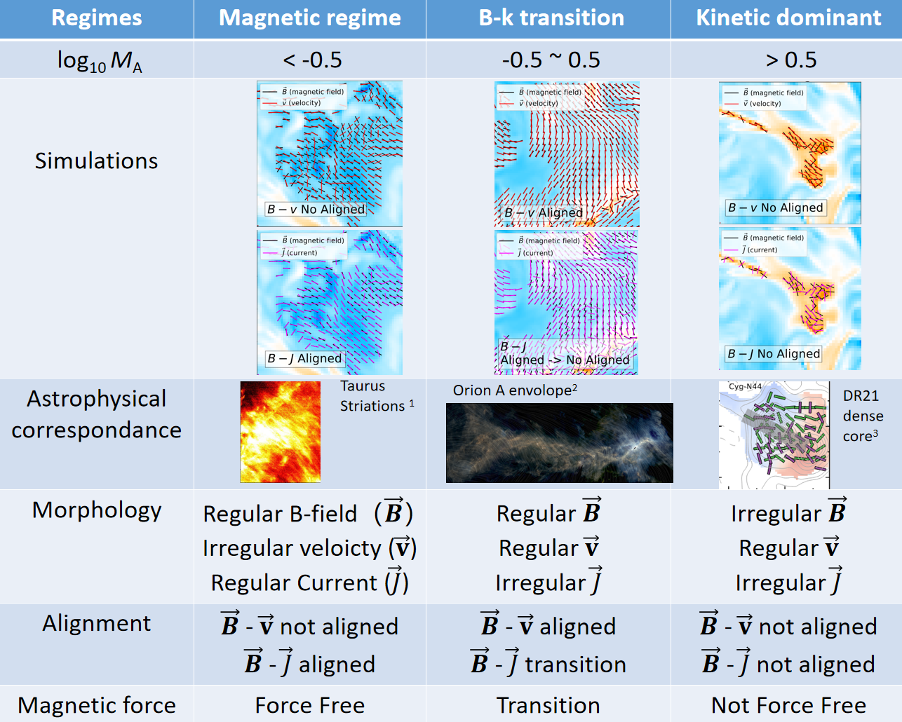
Figure 5: Summary of three regimes of compressive MHD turbulence. The Magnetic regime corresponds to observations in Heyer et al. (2016); Tritsis & Tassis (2016); Beattie et al. (2020); Skalidis et al. (2022). The B-k transition regime corresponds to observations in Hu et al. (2021); Zhao et al. (2022); Tram et al. (2023). The kinetic regime corresponds to observations toward Cyg N44 in Dr21 (Ching et al., 2018).

Figure 6: Relation between the Alfven Mach number $\cal{M}_{\rm A}$ and gas density $\rho$.

Appendix A Removing the projection effect in angle distributions

The probability density function, p($\theta$), of the angle between two vectors of random distribution is distributed in an N-dimensional space as:

$$p(\theta)=\frac{\Gamma(\frac{n}{2})}{\Gamma(\frac{n-1}{2})}\frac{{\rm sin}^{n-2}(\theta)}{\sqrt{\pi}}$$ (A1)

where n is numbers of dimensions, and $\theta$ is the angle between two vectors of random distribution. In our alignment analysis, we study the angle between qualities measured in 3D. When $n=3$, we have

$$p(\theta)=\frac{1}{2}{\rm sin}\theta\;,$$ (A2)

which two randomly-selected vectors have a alignment angle clustered at around $\theta=45^{\circ}$, caused by the projection effect. To remove the projection effect, we use the probability density function p($\theta$) to weight the angle distribution:

$$I(\theta_{\rm corrected})=I(\theta_{\rm original})/p(\theta)$$ (A3)

where $I(\theta_{\rm original})$ represents the original angle distribution and $I(\theta_{\rm corrected})$ represents the corrected angle distribution, with the projected effects removed.

Appendix B 2D slice of magnetic field, velocity and current

Fig. 7 shows the distribution of density $\rho$, velocity field $v$, magnetic field $B$, and current field $J$ in X-Y plane, which is a slice of 3D space.

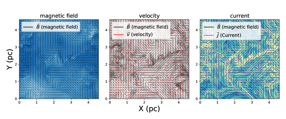
Figure 7: Distribution of magnetic field, velocity, current in the X-Y plane. The background and vector in the left panel are magnetic field strength and magnetic field orientation. The background in the middle panel is gas density. The black and red vectors display the orientation of the magnetic field and velocity. The background in the right panel is the strength of the current. The purple and black vectors present the magnetic field orientation and current orientation.

References

- Beattie et al. (2024) Beattie, J. R., Federrath, C., Klessen, R. S., Cielo, S., & Bhattacharjee, A. 2024, arXiv e-prints, arXiv:2405.16626, doi: 10.48550/arXiv.2405.16626
- Beattie et al. (2020) Beattie, J. R., Federrath, C., & Seta, A. 2020, MNRAS, 498, 1593, doi: 10.1093/mnras/staa2257
- Burkhart et al. (2015) Burkhart, B., Collins, D. C., & Lazarian, A. 2015, ApJ, 808, 48, doi: 10.1088/0004-637X/808/1/48
- Burkhart et al. (2020) Burkhart, B., Appel, S. M., Bialy, S., et al. 2020, ApJ, 905, 14, doi: 10.3847/1538-4357/abc484
- Ching et al. (2018) Ching, T.-C., Lai, S.-P., Zhang, Q., et al. 2018, ApJ, 865, 110, doi: 10.3847/1538-4357/aad9fc
- Collins et al. (2012) Collins, D. C., Kritsuk, A. G., Padoan, P., et al. 2012, ApJ, 750, 13, doi: 10.1088/0004-637X/750/1/13
- Collins et al. (2010) Collins, D. C., Xu, H., Norman, M. L., Li, H., & Li, S. 2010, ApJS, 186, 308, doi: 10.1088/0067-0049/186/2/308
- Frisch (1995) Frisch, U. 1995, Turbulence. The legacy of A.N. Kolmogorov, doi: 10.1017/CBO9781139170666
- Heyer et al. (2016) Heyer, M., Goldsmith, P. F., Yıldız, U. A., et al. 2016, MNRAS, 461, 3918, doi: 10.1093/mnras/stw1567
- Hu et al. (2021) Hu, Y., Lazarian, A., & Stanimirović, S. 2021, ApJ, 912, 2, doi: 10.3847/1538-4357/abedb7
- Hu et al. (2019) Hu, Y., Yuen, K. H., Lazarian, V., et al. 2019, Nature Astronomy, 3, 776, doi: 10.1038/s41550-019-0769-0
- Kolmogorov (1941) Kolmogorov, A. 1941, Akademiia Nauk SSSR Doklady, 30, 301
- Mac Low & Klessen (2004) Mac Low, M.-M., & Klessen, R. S. 2004, Reviews of Modern Physics, 76, 125, doi: 10.1103/RevModPhys.76.125
- Matthaeus et al. (2008) Matthaeus, W. H., Pouquet, A., Mininni, P. D., Dmitruk, P., & Breech, B. 2008, Phys. Rev. Lett., 100, 085003, doi: 10.1103/PhysRevLett.100.085003
- Padoan & Nordlund (2011) Padoan, P., & Nordlund, Å. 2011, ApJ, 730, 40, doi: 10.1088/0004-637X/730/1/40
- Pattle et al. (2023) Pattle, K., Fissel, L., Tahani, M., Liu, T., & Ntormousi, E. 2023, in Astronomical Society of the Pacific Conference Series, Vol. 534, Protostars and Planets VII, ed. S. Inutsuka, Y. Aikawa, T. Muto, K. Tomida, & M. Tamura, 193, doi: 10.48550/arXiv.2203.11179
- Pudritz et al. (2007) Pudritz, R. E., Ouyed, R., Fendt, C., & Brandenburg, A. 2007, in Protostars and Planets V, ed. B. Reipurth, D. Jewitt, & K. Keil, 277, doi: 10.48550/arXiv.astro-ph/0603592
- Skalidis et al. (2022) Skalidis, R., Tassis, K., Panopoulou, G. V., et al. 2022, A&A, 665, A77, doi: 10.1051/0004-6361/202142512
- Tram et al. (2023) Tram, L. N., Bonne, L., Hu, Y., et al. 2023, ApJ, 946, 8, doi: 10.3847/1538-4357/acaab0
- Tritsis & Tassis (2016) Tritsis, A., & Tassis, K. 2016, MNRAS, 462, 3602, doi: 10.1093/mnras/stw1881
- Zhao et al. (2022) Zhao, M., Zhou, J., Hu, Y., et al. 2022, ApJ, 934, 45, doi: 10.3847/1538-4357/ac78e8