Proper Wilson flow time for calculating the topological charge density and the pseudoscalar glueball mass in quenched lattice QCD

Abstract

The proper flow time for the Wilson flow in calculating the topological charge, topological susceptibility, and topological charge density correlator (TCDC) using the gluonic definition is analyzed. The proper flow time for the topological charge and TCDC is determined by different methods. The proper flow time may vary depending on whether the calculation is for the topological charge, topological density, topological susceptibility, or TCDC. Specifically, the flow time identified using the matching procedure is optimal for TCDC and a good choice for the topological susceptibility. Additionally, the pseudoscalar glueball is extracted from the TCDC using the bosonic definition at the identified proper flow time for three ensembles, and the continuum mass value is obtained through continuous extrapolation.

I Introduction

The QCD vacuum is believed to possess a non-trivial topological structure, characterized by the topological charge and topological charge density. These topological properties are crucial for understanding various phenomena, including the $\text{U}\left(1\right)_{A}$ problem, confinement, $\theta$ dependence, and spontaneous chiral symmetry breaking Schierholz:1994pb ; Witten:1978bc ; Diakonov:1995ea . Lattice QCD is a powerful tool for investigating these topological properties from first principles. Definitions of topological charge and topological charge density are generally divided into the fermionic and gluonic definitions Cichy:2014qta ; Muller-Preussker:2015daa ; Alexandrou:2017hqw . On the lattice, results of the gluonic and fermionic definitions of the topological charge are consistent in the continuum limit $a\to 0$ Belavin:1975fg ; Fujikawa:1998if ; Kikukawa:1998pd . The topological charge calculated using the fermionic definition is an integer Atiyah:1971rm ; Hasenfratz:1998ri ; however, the computational cost of this method is prohibitively high. Computing the topological charge on the lattice using the gluonic definition is less computationally demanding, but the numerical value of the topological charge is typically not an integer due to ultraviolet fluctuations in the gauge fields. To ensure that the numerical value of the topological charge nears an integer, a renormalization constant must be applied, or smoothing techniques must be used. Smoothing procedures, such as cooling, smearing (including APE, HYP, and stout smearing), or gradient flow, are commonly employed in the computation of the topological charge density Alexandrou:2017hqw . However, determining the optimal level of smoothing in the calculation of the topological charge or topological charge density is a critical issue. By analyzing the relationship between the topological charge of the clover-Dirac operator and the nearest integer, Ref. Chiu2019 provides a lower bound for calculating the topological charge. The topological susceptibility and topological charge density correlation (TCDC) are also important research subjects in studying the vacuum’s topological properties.

TCDC is negative at any non-zero distances due to the reflection positivity and the pseudoscalar nature of the relevant local operator in Euclidean field theory. The negativity of the TCDC has significant implications for the nature of the topological charge structure in the QCD vacuum Chowdhury:2012sq . For instance, the pseudoscalar glueball mass can be extracted from the TCDC in pure gauge theory. The correlator of gluonic observables exhibits large vacuum fluctuations, making the extraction of glueball masses significantly more challenging compared to hadronic masses. However, extracting the pseudoscalar glueball mass from the TCDC does not require calculating connected and disconnected quark diagrams Creutz:2010ec . In lattice QCD, due to severe singularities and lattice artifacts in the TCDC, smoothing of the gauge field is necessary. It is well known that undersmearing cannot completely remove lattice artifacts, while oversmearing may wipe out even the negative nature of the correlator Chowdhury:2014mra . Therefore, a lower bound on the smoothing (Wilson flow) is required.

The topological susceptibility $\chi$ can be obtained by the four-volume integral of the TCDC Smit:1986fn . Topological susceptibility, which reflects the fluctuations of the topological charge, is of great importance in the study of the QCD vacuum. The universality of the topological susceptibility in the fermionic definition shows that it is free of short-distance singularities Luscher:2010ik . The topological susceptibility $\chi$ is linked to the $\text{U}\left(1\right)$ anomaly and the mass of the flavor-singlet pseudoscalar $\eta^{\prime}$ meson in pure Yang-Mills theory, as expressed in the well-known Witten-Veneziano relation Witten:1979vv ; Veneziano:1979ec . Additionally, a lower bound for the proper flow time of the Wilson flow can be determined by using the topological susceptibility Mazur:2020hvt .

The overlap operator, as a solution to the Ginsparg-Wilson equation Neuberger:1997fp ; Neuberger:1998wv , is commonly used to calculate the topological charge of the fermionic definition. The topological charge computed using the overlap operator is an exact integer. Traditionally, the topological charge density has been calculated by using the point source Horvath:2003yj ; Ilgenfritz:2007xu , which is almost impossible on a large volume lattice. To address this, Ref. Xiong:2019pmh proposed the symmetric source (SMP) method to calculate the topological charge density of the fermionic definition. Although the SMP method can reduce the computational resources required for calculating the topological charge, it remains challenging to apply the SMP method for calculating the topological susceptibility or TCDC in the context of when the number of configurations is large. In current practical calculations, we generally use the gluonic definition for the topological charge density to compute the topological susceptibility or TCDC. However, the degree of smoothing in the calculation of the bosonic definition for the topological charge density remains an unresolved issue. Three matching methods are considered in this paper. The first method is to find the most matching topological charge in the calculation of the topological charge. The second method is to calculate the matching parameter and determine the flow time at which this parameter is closest to 1. The third method involves identifying the minimum flow time at which the topological susceptibility reaches a plateau.

The matching parameters for different settings of the SMP method, as well as those obtained by comparing the SMP method with the Wilson flow results, will be calculated. By analyzing these matching parameters, the proper flow time for calculating the TCDC will be determined. Further exploration of the SMP method in the calculation of the topological charge of the fermionic definition will be presented. The relationship between the TCDC and topological susceptibility with the matching parameters will be discussed. Additionally, an attempt will be made to extract the pseudoscalar glueball mass from the TCDC at the proper flow time.

II Simulation setup

The L scher-Weisz gauge action is used to generate the pure gauge lattice configurations. This gauge action is tadpole-improved at tree-level $\mathcal{O}\left(a^{2}\right)$ and combines the plaquette and rectangle gauge actions, implemented using the pseudo-heat-bath algorithm Luscher:1984xn ; Bonnet:2001rc . The parameters of the ensembles used to generate configurations with periodic boundary conditions are detailed in Tab. 1, and the lattice spacings $a$ are determined through the Wilson flow.

$\beta$	$L^{3}\times T$	$N_{\text{conf}}$	$a\left(\text{fm}\right)$
$4.5$	$16^{4}$	$2000$	$0.1287\left(4\right)$
$4.8$	$24^{3}\times 48$	$2000$	$0.0896\left(1\right)$
$5.0$	$32^{4}$	$1500$	$0.0660\left(2\right)$

Table 1: Simulation parameters of configurations used. $N_{\text{conf}}$ is the total number of configurations in the ensemble.

The same overlap operator as in Ref. Cheng:2020bql is used to calculate the topological charge density of the fermionic definition, and the parameter $\kappa$ is the input variable. In this work, we specifically choose $\kappa=0.18$ and $0.19$. While the topological charge computed using this overlap operator with the point sources yields an integer value, the computational cost is significantly high. To reduce the computational cost, the symmetric multi-probing source (SMP) method is introduced to calculate the topological charge density with the Dirac operator Xiong:2019pmh . The SMP method is utilized to calculate the topological charge density of the fermionic definition, as follows:

$$q_{\text{smp}}\left(x\right) =\sum_{\alpha,a}\psi\left(x,\alpha,a\right)\left(\tilde{D}_{\text{ov}}\left(x\right)\right)\phi_{P}\left(S\left(x,P\right),\alpha,a\right)$$

$$=\sum_{\alpha,a}\psi\left(x,\alpha,a\right)\left(\tilde{D}_{\text{ov}}\left(x\right)\right)\psi\left(x,\alpha,a\right),$$ (1)

and the corresponding topological charge is

$$Q_{\text{smp}}=\sum_{x}q_{\text{smp}}\left(x\right),$$ (2)

where $\phi_{P}\left(S\left(X,P\right),\alpha,a\right)$ represents the SMP source vector with $(d,\text{mode})$, and other parameters in the SMP source vector are explained in Ref. Cheng:2020bql . The total number of SMP source vectors $\phi_{P}\left(S\left(X,P\right),\alpha,a\right)$ for the $(d,\text{mode})$ is

$$N_{\text{SMPV}}=\begin{cases}d^{4},&\text{mode}=0,\\ 2d^{4},&\text{mode}=1,\\ \frac{d^{4}}{2},&\text{mode}=2,\end{cases}$$

and which can cover all grid points is $12N_{\text{SMPV}}$. We use $(d,\text{mode})$ to represent the number of SMP source vectors in the following. Under a proper scheme $P$ of the SMP method, we can obtain the expected topological charge density.

The field tensor used in calculating the topological charge density of the gluonic definition is a 3-loop $\mathcal{O}\left(a^{4}\right)$-improved and defined as BilsonThompson:2002jk ,

$$F_{\mu\nu}^{\text{Imp}}=\frac{27}{18}C_{\text{$\mu\nu$}}^{\left(1,1\right)}-\frac{27}{180}C_{\text{$\mu\nu$}}^{\left(2,2\right)}+\frac{1}{90}C_{\text{$\mu\nu$}}^{\left(3,3\right)},$$ (3)

and $C_{\mu\nu}^{\left(m,m\right)}$ is the clover term constructed by $m\times m$ loops. The Wilson flow is used to smooth the gauge field in the gluonic definition, and the gauge fields do not need to be renormalized. The topological charge density of the gluonic definition by using the Wilson flow is

$${{q}_{\text{wf}}}\left(x\right)=\frac{1}{32{{\pi}^{2}}}{{\varepsilon}_{\mu\nu\rho\sigma}}\text{Tr}\left[F_{\mu\nu}^{\text{Imp}}\left(x\right)F_{\rho\sigma}^{\text{Imp}}\left(x\right)\right],$$ (4)

and the corresponding topological charge $Q_{\text{wf}}$ for the gluonic definition is given by

$$Q_{\text{wf}}=\sum\limits_{x}{{{q}_{\text{wf}}}}\left(x\right).$$ (5)

To determine the proper flow time $\tau_{\text{qpr}}$ for calculating the topological charge using the gluonic definition, we introduce a new comparing method by identifying the minimum value of the absolute difference between the topological charge obtained from the fermionic definition and that calculated from the gluonic definition at various Wilson flow time. This process involves finding the minimum value of the following expression for different Wilson flow times:

$$\text{min}\left|Q-Q_{\text{wf}}\right|,$$ (6)

where $Q$ is the topological charge obtained by rounding the topological charge $Q_{\text{smp}}$ calculated using the SMP method to the nearest integer, and $Q_{\text{wf}}$ represents the topological charge of the gluonic definition by using the Wilson flow.

To investigate how to use the SMP method to determine the proper flow time $\tau_{\text{pr}}$ when computing the topological charge density of the gluonic definition, a matching procedure is introduced. The matching quantity $\Xi_{AB}$ will be calculated as follows Bruckmann:2006wf ; Moran:2010rn ,

$$\Xi_{AB}=\frac{\chi_{AB}^{2}}{\chi_{AA}\chi_{BB}},$$ (7)

with

$$\chi_{AB}=\frac{1}{V}\sum_{x}\left(q_{A}\left(x\right)-\bar{q}_{A}\right)\left(q_{B}\left(x\right)-\bar{q}_{B}\right),$$ (8)

where $\bar{q}$ is the mean value of topological charge density $q\left(x\right)$, and $V$ is the volume. When the numerical value of $\Xi_{AB}$ is nearest to $1$, the flow time is the desired proper Wilson flow time $\tau_{\text{pr}}$.

III The matching parameter and the proper flow time of the Wilson flow

In Ref. Cheng:2020bql , the results indicate that the outcomes of the SMP method with parameters $(8,0)$ can serve as a benchmark for calculating the matching parameter $\Xi_{AB}$. To compare results from different parameters $(d\neq 8,\text{mode}\neq 0)$ with those obtained using the parameter set $(8,0)$ in the SMP method, the matching parameters $\Xi_{AB}$ are computed for various hopping parameters $\kappa$. Given the constraints of computational resources, only three configurations are analyzed for each lattice ensemble in the SMP method.

Lattice	# of conf.	$\left(2,0\right)$	$\left(2,1\right)$	$\left(4,2\right)$	$\left(4,0\right)$	$\left(4,1\right)$
$16^{4}$	$10$	$0.638631$	$0.819229$	$0.976946$	$0.988357$	$0.999246$
	$20$	$0.630302$	$0.814710$	$0.976150$	$0.987895$	$0.999242$
	$30$	$0.625374$	$0.812900$	$0.976215$	$0.988113$	$0.999250$
$24^{3}\times 48$	$5$	$0.622905$	$0.811863$	$0.978178$	$0.988439$	$0.999436$
	$15$	$0.621431$	$0.811156$	$0.978089$	$0.988359$	$0.999436$
	$30$	$0.622252$	$0.812087$	$0.978154$	$0.988425$	$0.999437$
$32^{4}$	$25$	$0.617173$	$0.810155$	$0.978567$	$0.988435$	$0.999472$
	$40$	$0.619947$	$0.811330$	$0.978676$	$0.988496$	$0.999475$
	$50$	$0.618602$	$0.810218$	$0.978552$	$0.988459$	$0.999470$

Table 2: $\Xi_{AB}$ for different parameters $(d\neq 8,\text{mode}\neq 0)$ of the SMP method compared to $\left(8,0\right)$. The hopping parameter is $\kappa=0.18$. # of conf. stands for the sequence number of configurations.

The results for $16^{4}$, $24^{3}\times 48$, and $32^{4}$ with $\kappa=0.18$ are shown in Tab. 2. In Tab. 3, the results for $16^{4}$ and $24^{3}\times 48$ with $\kappa=0.19$ are presented. However, due to computational resource limitations, the results for $\kappa=0.19$ in the lattice $32^{4}$ were not computed. When the SMP parameters are $(4,2)$, the matching parameters are already very close to $1$, indicating that the topological charge density calculated with parameters $(4,2)$ can also be used to determine the matching parameter $\Xi_{AB}$. Using the SMP method with parameters $(4,2)$ requires approximately $1/32$ of the computational resources compared to the parameters $(8,0)$, or $1/512$ of the computational resources compared to the point sources, leading to significant resource savings.

Lattice	# of conf.	$\left(2,0\right)$	$\left(2,1\right)$	$\left(4,2\right)$	$\left(4,0\right)$	$\left(4,1\right)$
$16^{4}$	$10$	$0.681956$	$0.853189$	$0.984066$	$0.991147$	$0.999579$
	$20$	$0.671241$	$0.847403$	$0.983229$	$0.990655$	$0.999558$
	$30$	$0.666107$	$0.844403$	$0.983037$	$0.990749$	$0.999552$
$24^{3}\times 48$	$5$	$0.649081$	$0.833534$	$0.982238$	$0.990288$	$0.999565$
	$15$	$0.647766$	$0.832886$	$0.982189$	$0.990227$	$0.999564$
	$30$	$0.648395$	$0.833703$	$0.982230$	$0.990281$	$0.999565$

Table 3: $\Xi_{AB}$ for different parameters $\left(d\neq 8,\text{mode}\neq 0\right)$ of the SMP method compared with $\left(8,0\right)$ and $\kappa=0.19$. Considering the limitations of computational resources, the results of the lattice $32^{4}$ were not computed. # of conf. is the sequence number of configurations.

In Fig. 1, the matching parameter results obtained by comparing the topological charge density calculated using the SMP method with that calculated using the Wilson flow method are presented. The results indicate that as the number of SMP source vectors increases, the value of the matching parameter $\Xi_{AB}$ also increases. However, even when the number of SMP source vectors exceeds the source vector count at the parameters $(4,2)$, the increase in the matching parameters is no longer significant. This suggests that the parameters $(4,2)$ in the SMP method are sufficient for calculating the matching parameters when comparing the SMP method with Wilson flow. Additionally, the proper flow time remains essentially constant, regardless of variations in the parameters (d, mode) within the SMP method. The proper flow time in the calculation of topological density in the gluonic definition can be obtained from the matching procedure. All results indicate that choosing the parameters $(4,2)$ in the SMP method is a good option when selecting a benchmark to determine the matching parameter $\Xi_{AB}$.

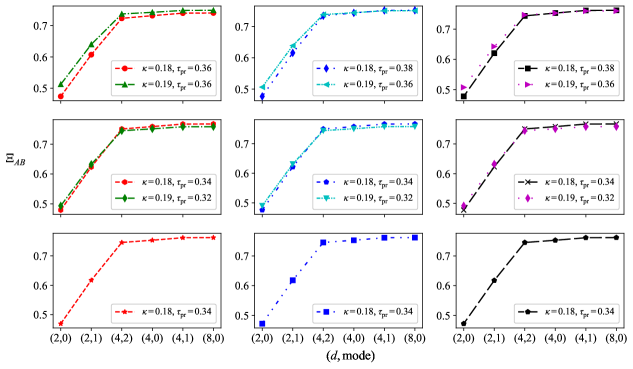
Figure 1: The best $\Xi_{AB}$ for SMP with different parameters $\left(d,\text{mode}\right)$ compared with the Wilson flow in the calculation of topological charge density. $\tau_{\text{pr}}$ is the proper flow time, and $\kappa$ is the hopping parameter. From top to bottom, the results for the lattices $16^{4}$, $24^{3}\times 48$, and $32^{4}$ are presented. The results of different configurations for each lattice are shown from left to right.

We adopt the matching results at $\kappa=0.18$. In the calculation of the topological charge density, the proper flow time for lattices of $16^{4}$ at $\beta=4.5$, $24^{3}\times 48$ at $\beta=4.8$ and $32^{4}$ at $\beta=5.0$ are approximately $\tau=0.38$, $\tau=0.34$ and $\tau=0.34$. The corresponding proper flow radii of the Wilson flow $\sqrt{8\tau_{\text{pr}}}=0.224$, $0.148,$ and $0.109\thinspace\text{fm}$, respectively. In the subsequent calculation of TCDC, this proper flow time $\tau_{\text{pr}}$ will be used in the Wilson flow.

The topological charges $Q$ obtained using the SMP method with different parameters $\left(d,\text{mode}\right)$ and the Wilson flow method at the proper flow time $\tau_{\text{pr}}$ are illustrated in Fig. 2. The results indicate that as the number of SMP source vectors increases, the topological charges $Q$ calculated by the SMP method approach integer values, aligning with expectations. Notably, when the parameters of the SMP source vectors are set to $(4,2)$, the topological charge $Q$ derived from the fermionic definition using the SMP method closely matches that calculated from point sources. These findings indicate that using SMP sources with parameters $(4,2)$ could be a viable approach for calculating the topological charge of the fermionic definition, potentially reducing computational resource requirements compared to traditional point source calculations. All results suggest that the SMP method with parameters $(4,2)$ could be considered for application to the computation of TCDC and the topological susceptibility of the fermionic definition.

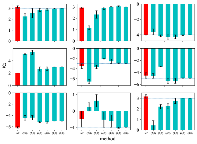
Figure 2: The topological charge $Q$ of configurations obtained using the SMP method with different parameters $\left(d,\text{mode}\right)$ and the Wilson flow. wf stands for the Wilson flow at $\tau_{\text{pr}}$. The results for the lattices $16^{4}$, $24^{3}\times 48$, and $32^{4}$ are presented from top to bottom, and the configurations for each lattice are shown from left to right.

However, the topological charges of the gluonic definition, calculated at the proper flow time $\tau_{\text{pr}}$ through the matching procedure, deviate considerably from integer values. The upcoming research will demonstrate that the proper flow time determined by the matching method is not suitable for the calculation of topological charge, it is applicable for the calculation of TCDC. For calculating the topological charge of the gluonic definition using the Wilson flow, the proper flow time can be determined using the eq. (6).

In Tab. 4, the topological charge calculated using the SMP method with parameters $(8,0)$ and the Wilson flow, along with the proper flow time $\tau_{\text{qpr}}$ for the gluonic definition, are presented. The value of $Q$ is obtained by rounding the topological charge $Q_{\text{smp}}$, calculated using the SMP method with parameters $(8,0)$, to the nearest integer. The proper flow time $\tau_{\text{qpr}}$ for calculating $Q_{\text{wf}}$ using the eq. (5) is determined by identifying the minimum value of the absolute difference between $Q$ and $Q_{\text{wf}}$ as outlined in eq. (6).

Lattice	# of conf.	$Q$	$Q_{\text{smp}}$	$\left|Q-Q_{\text{smp}}\right|$	$Q_{\text{wf}}$	$\left|Q-Q_{\text{wf}}\right|$	$\tau_{\text{qpr}}$
$16^{4}$	$10$	$3$	$3.0002$	$0.0002$	$2.9823$	$0.0177$	$0.40$
	$20$	$3$	$3.0019$	$0.0019$	$3.0365$	$0.0365$	$0.40$
	$30$	$-4$	$-4.0045$	$0.0045$	$-4.0206$	$0.0206$	$0.38$
$24^{3}\times 48$	$5$	$3$	$3.0028$	$0.0028$	$2.9521$	$0.0479$	$1.00$
	$15$	$-3$	$3.0021$	$0.0021$	$-2.9871$	$0.0129$	$0.26$
	$30$	$-5$	$-4.9933$	$0.0067$	$-4.9756$	$0.0244$	$0.44$
$32^{4}$	$25$	$-5$	$-5.0033$	$0.0033$	$-5.0165$	$0.0165$	$1.00$
	$40$	$-1$	$-0.9987$	$0.0013$	$-0.9974$	$0.0026$	$0.24$
	$50$	$3$	$2.9963$	$0.0037$	$3.0008$	$0.0008$	$1.00$

Table 4: The proper flow time $\tau_{\text{qpr}}$ for the topological charge $Q_{\text{wf}}$ calculated using the Wilson flow. $Q$ is obtained by rounding the result of the SMP method with parameters $(8,0)$ to the nearest integer. # of conf. is the sequence number of the configuration.

The results demonstrate that the topological charge derived from the SMP method with parameters $(8,0)$ is numerically very close to the precise value obtained from point sources, indicating that $Q$ accurately represents the topological charge of the configuration. Furthermore, it suggests that a larger Wilson flow time is generally necessary when calculating the topological charge for the gluonic definition. This also indicates that the proper flow time $\tau_{\text{pr}}$ determined by the matching method may not be the optimal choice to calculate the topological charge of the gluonic definition.

The topological charge calculated using the SMP method with parameters $(4,2)$ and the Wilson flow, along with the proper flow time $\tau_{\text{qpr}}$ for the topological charge of the gluonic definition, is presented in Tab. 5. The methods for determining $Q$ and $\tau_{\text{qpr}}$ are the same as those employed in Tab. 4. The values of $Q$ and $\tau_{\text{qpr}}$ obtained using the SMP method with parameters $(4,2)$ are fundamentally similar to those derived with parameters $(8,0)$.

Lattice	# of conf.	$Q$	$Q_{\text{smp}}$	$\left|Q-Q_{\text{smp}}\right|$	$Q_{\text{wf}}$	$\left|Q-Q_{\text{wf}}\right|$	$\tau_{\text{qpr}}$
$16^{4}$	$10$	$3$	$2.8563$	$0.1437$	$2.9823$	$0.0177$	$0.40$
	$20$	$3$	$2.8864$	$0.1136$	$3.0365$	$0.0365$	$0.40$
	$30$	$-4$	$-4.2867$	$0.2867$	$-4.0206$	$0.0206$	$0.38$
$24^{3}\times 48$	$5$	$3$	$2.6528$	$0.3472$	$2.9521$	$0.0479$	$1.00$
	$15$	$-2$	$-2.0643$	$0.9357$	$-2.1213$	$0.8787$	$0.18$
	$30$	$-5$	$-5.4482$	$0.4482$	$-4.9756$	$0.0244$	$0.44$
$32^{4}$	$25$	$-5$	$-5.1343$	$0.1343$	$-5.0165$	$0.0165$	$1.00$
	$40$	$-1$	$-0.5291$	$0.4709$	$-0.9974$	$0.0026$	$0.24$
	$50$	$2$	$2.2644$	$0.7356$	$3.0008$	$0.0008$	$1.00$

Table 5: The proper flow time $\tau_{\text{qpr}}$ for calculating $Q$ of the gluonic definition. $Q$ is obtained by rounding the result of the SMP method with parameters $(4,2)$ to the nearest integer. # of conf. stands for the sequence number of configurations.

These results indicate that the SMP method with parameters $(4,2)$ is indeed a viable approach for accurately determining the topological charge of the fermionic definition. Moreover, this method can effectively establish the proper flow time $\tau_{\text{qpr}}$ when calculating the topological charge of the gluonic definition using the Wilson flow. By analyzing the index of the overlap-Dirac operator concerning the clover topological charge during the Wilson flow, Ref. Chiu2019 shows that max $\{t_{c}\}\sim 77$ for the Wilson flow. This max $\{t_{c}\}\sim 77$ corresponds to a lower bound for the Wilson flow time of $\tau\sim 0.77$, which is compatible with our results. Notably, the results show that when calculating the topological charge of the gluonic definition, the proper flow time $\tau_{\text{qpr}}$ is generally larger than $\tau_{\text{pr}}$. The results in the next section will demonstrate that when calculating TCDC at the proper flow time $\tau_{\text{qpr}}$, TCDC may exhibit oversmearing, meaning that the negative dip of TCDC may disappear, as shown in Fig. 3.

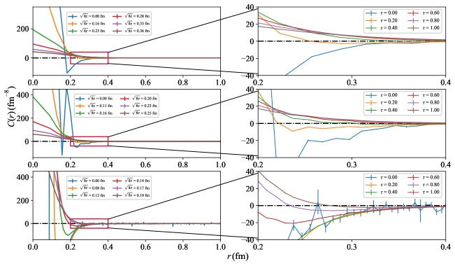
Figure 3: $C\left(r/a\right)$ v.s. $r$ for different lattices. From top to bottom, the results for $16^{4}$ with $\beta=4.5$, $24^{3}\times 48$ with $\beta=4.80$, and $32^{4}$ with $\beta=5.0$ are presented. $\sqrt{8\tau}$ is the flow radius of the Wilson flow time $\tau$.

IV The topological charge density correlator and the pseudoscalar glueball mass

TCDC is defined as

$$C\left(r\right)=\left\langle q\left(x\right)q\left(0\right)\right\rangle,\thinspace\thinspace\thinspace\thinspace r=\left|x\right|,$$ (9)

and the four-volume integral of the TCDC gives the topological susceptibility

$$\chi=\int\text{d}^{4}x\left\langle q\left(x\right)q\left(0\right)\right\rangle=\frac{\left\langle Q^{2}\right\rangle}{V},\thinspace\thinspace\thinspace\thinspace V\to\infty.$$ (10)

Due to the presence of severe singularities and lattice artifacts in TCDC, a smoothing procedure is essential to refine the gauge fields. In this study, we employ the Wilson flow method for this purpose. Undersmearing fails to adequately eliminate the lattice artifacts, while oversmearing can erase even the negative character of the TCDC, as illustrated in Fig. 3. The results indicate that the flow times at which the negative dip disappears at a distance of $r\sim 0.3\,\text{fm}$ are $\tau\approx 0.4$ for $16^{4}$, $\tau\approx 0.6$ for $24^{3}\times 48$, and $\tau\approx 1.0$ for $32^{4}$, which are very close to the corresponding $\tau_{\text{qpr}}$. In other words, when using the Wilson flow method to calculate TCDC at $\tau_{\text{qpr}}$, TCDC may be oversmearing.

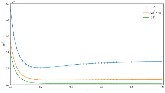
Figure 4: $\chi$ for ensembles $16^{4}$ with $\beta=4.50$, $24^{3}\times 48$ with $\beta=4.80$ and $32^{4}$ with $\beta=5.0$. $\tau$ is the Wilson flow time for the gluonic definition.

To determine the suitable Wilson flow time, Ref. Mazur:2020hvt suggests using the stability of the topological susceptibility to establish a lower bound for the Wilson flow time at finite temperature. The topological susceptibility $\chi$ for various lattices with respect to the Wilson flow time $\tau$ is presented in Fig. 4. As the flow time $\tau$ increases, UV fluctuations are gradually smoothed out, and the topological susceptibility eventually stabilizes, reaching a plateau around $\tau\approx 0.2$. This result suggests that the proper flow time $\tau_{\text{ps}}$, based on the stability of the topological susceptibility $\chi$, should be $\tau_{\text{ps}}=0.2$, which is smaller than the proper flow times $\tau_{\text{pr}}\approx 0.38$ and $0.34$ obtained through the matching procedures discussed in the previous section. All results demonstrate that the relationship between the proper flow times in the calculations of topological charge, TCDC, and topological susceptibility is given by $\tau_{\text{qpr}}>\tau_{\text{pr}}>\tau_{\text{ps}}$. This discrepancy may arise from the cumulative summation process or lattice artifacts, warranting further investigation.

The results indicate that while the topological susceptibility has stabilized at a Wilson flow time of $\tau=0.2$, significant fluctuations in the TCDC persist, as illustrated in Fig. 3. This suggests that the proper flow time $\tau_{\text{ps}}$ determined by susceptibility is not sufficient to calculate the TCDC optimally. In other words, when determining the TCDC of the gluonic definition, the required Wilson flow time is longer than $\tau_{\text{ps}}$ determined by the topological susceptibility. However, the TCDC calculated by Wilson flow at the proper flow time $\tau_{\text{pr}}$ retains the negative core part while achieving effective smoothing. This highlights the importance of selecting the proper Wilson flow time $\tau_{\text{pr}}$. Therefore, $\tau_{\text{pr}}$ is a optimal choice for the calculation of TCDC, and a good choice for the topological susceptibility in the gluonic definition. In this work, the calculation of TCDC will be performed using the Wilson flow method at the proper flow time $\tau_{\text{pr}}$.

TCDC can be used to extract the lowest pseudoscalar glueball mass in the negative region by the following form

$$\left\langle q\left(x\right)q\left(0\right)\right\rangle=\frac{m}{4\pi^{2}r}K_{1}\left(mr\right),$$ (11)

and $K_{1}\left(z\right)$ is a modified Bessel function, which has the asymptotic form Shuryak:1994rr

$$K_{1}\left(z\right)\underset{\text{large}\thinspace z}{\sim}e^{-z}\sqrt{\frac{\pi}{2z}}\left[1+\frac{3}{8z}\right].$$ (12)

We aim to extract the glueball mass from the TCDC of three ensembles using the Wilson flow at the proper flow time $\tau_{\text{pr}}$. To do this, we apply Eqs. (11) and (12) to determine the pseudoscalar glueball mass in the negative region. In this fitting procedure, both the amplitude and mass are treated as free parameters, and the ${{{\chi}^{2}}}/{\text{dof}}\;$ is calculated to evaluate the quality of the fit. It shows that the extracted mass remains independent of the endpoint once the error bars of the tail of the TCDC approach zeroChowdhury:2014mra ; Zou:2018mxc . The fitting is considered optimal when the value of ${{{\chi}^{2}}}/{\text{dof}}\;$ is closest to $1$. Consequently, we fix the endpoint and vary the starting point to extract the mass. The TCDC and the best-fitting curve for the ensemble $24^{3}\times 48$ with $\tau=0.34$ (or $\sqrt{8\tau}=0.15\thinspace\text{fm}$) as an example are illustrated in Fig. 5.

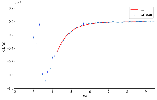
Figure 5: $C\left(r/a\right)$ versus $r$ at the Wilson flow time $\tau=0.34$. The fitting curve to extract the pseudoscalar glueball mass is also shown.

The optimal fit results for the three ensembles reveal minimal differences, as shown in Tab. 6. To obtain the particle mass via continuous extrapolation, we perform a constant fit. The plot of mass $M$ versus $a^{2}$, along with the fitting results, is illustrated in Fig. 6. The red solid line represents the mass of the pseudoscalar glueball, while the magenta lines indicate the associated errors. The mass of the pseudoscalar glueball, obtained through continuous extrapolation, is $m=2561\left(39\right)\text{MeV}$, consistent with the findings in Ref. Chowdhury:2014mra ; Chen:2005mg .

$L^{3}\times T$	Fitting interval$\thinspace\left(\text{fm}\right)$	$am$	$m\thinspace\left(\text{MeV}\right)$	$\chi^{2}/{\text{dof}}$
$16^{4}$	$\left[0.446,1.013\right]$	$1.663\left(75\right)$	$2550\left(116\right)$	$0.846$
$24^{3}\times 48$	$\left[0.380,0.801\right]$	$1.161\left(20\right)$	$2558\left(58\right)$	$0.979$
$32^{4}$	$\left[0.396,0.650\right]$	$0.864\left(37\right)$	$2585\left(111\right)$	$1.002$

Table 6: The fitting detailed parameters from TCDC for different ensembles.

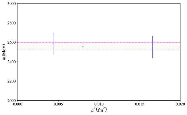
Figure 6: The colored scatter points represent the particle masses obtained from curve fitting across different lattice ensembles. The red solid line shows the continuum value of the pseudoscalar glueball mass, and the magenta lines indicate the errors.

V Conclusions

The topological charge density of lattice QCD using both the fermionic and gluonic definitions is analyzed in this paper. The topological charge density for the fermionic definition is calculated using the SMP method, while the gluonic definition employs the Wilson flow. The SMP method offers advantages in computing the topological charge for the fermionic definition compared to the point sources, particularly with the parameters $(4,2)$, which is used effectively to compute the topological charge of the fermionic definition and significantly reduce computational resource requirements. The SMP method with parameters $(4,2)$ offers a potential approach for calculating TCDC and the topological susceptibility of the fermionic definition. The SMP method with parameters $(4,2)$ can be used to determine the proper flow time $\tau_{\text{pr}}$.

We investigate the proper flow time for calculating the topological charge, topological susceptibility, and the TCDC of the gluonic definition using the Wilson flow. It is important to note that the proper flow time may differ when calculating the topological charge, topological charge density, topological susceptibility, and TCDC using the Wilson flow method. Specifically, the flow time for calculating the topological charge is the longest, followed by the time for TCDC, with the shortest time allocated for the topological susceptibility.

By identifying the topological charge calculated via the Wilson flow that is closest to that determined by the SMP method, we can ascertain the proper flow time $\tau_{\text{qpr}}$ for the calculation of the topological charge of the gluonic definition. The proper flow time $\tau_{\text{ps}}$ for calculating the topological susceptibility using the Wilson flow is identified as the point at which the susceptibility no longer decreases with increasing flow time. However, both $\tau_{\text{ps}}$ and $\tau_{\text{qpr}}$ are not suitable for calculating TCDC. The proper flow time $\tau_{\text{pr}}$ can indeed be determined using the matching parameter $\Xi_{AB}$. $\tau_{\text{pr}}$ is the optimal choice for calculating TCDC and a good choice for the topological susceptibility.

The TCDC of the gluonic definition has also been analyzed using the Wilson flow in this work. Given its severe singularities and lattice artifacts, the Wilson flow serves as an effective smoothing method. We employ the TCDC calculated at the proper flow time to extract the pseudoscalar glueball mass through curve fitting. The pseudoscalar glueball mass obtained from the continuous extrapolation of three ensembles is consistent with results from other studies.

Given limitations in computational resources, the results of this study are preliminary, particularly regarding the determination of the proper flow time and the continuous extrapolation of particle masses. In the future, we should use more lattice ensembles, larger lattice volumes, or more configurations to further investigate this issue. Additionally, we may consider improving the method for determining the proper flow time to enhance the accuracy and effectiveness of the calculations.

- (1) G. Schierholz, Towards a dynamical solution of the strong CP problem, Nucl. Phys. Proc. Suppl. 37A (1994) 203–210 [hep-lat/9403012].
- (2) Edward Witten, Instantons, the Quark Model, and the 1/N Expansion, Nucl. Phys. B 149 (1979) 285–320.
- (3) Dmitri Diakonov, Chiral symmetry breaking by instantons, Proc. Int. Sch. Phys. Fermi 130 (1996) 397–432 [hep-ph/9602375].
- (4) Krzysztof Cichy, Arthur Dromard, Elena Garcia-Ramos, Konstantin Ottnad, Carsten Urbach, Marc Wagner, Urs Wenger, and Falk Zimmermann, Comparison of different lattice definitions of the topological charge, PoS LATTICE2014 (2014) 075 [hep-lat/1411.1205].
- (5) M. Müller-Preussker, Recent results on topology on the lattice (in memory of Pierre van Baal), PoS LATTICE2014 (2015) 003 [hep-lat/1503.01254].
- (6) Constantia Alexandrou, Andreas Athenodorou, Krzysztof Cichy, Arthur Dromard, Elena Garcia-Ramos, Karl Jansen, Urs Wenger, and Falk Zimmermann, Comparison of topological charge definitions in Lattice QCD, Eur. Phys. J. C 80 (2020) 424 [hep-lat/1708.00696].
- (7) A.A. Belavin, Alexander M. Polyakov, A.S. Schwartz, and Yu.S. Tyupkin, Pseudoparticle Solutions of the Yang-Mills Equations, Phys. Lett. B 59 (1975) 85–87.
- (8) Kazuo Fujikawa, A continuum limit of the chiral jacobian in lattice gauge theory, Nucl. Phys. B 546 (1999) 480–494.
- (9) Yoshio Kikukawa and Atsushi Yamada, Weak coupling expansion of massless QCD with a Ginsparg-Wilson fermion and axial U(1) anomaly, Phys. Lett. B 448 (1999) 265–274 [hep-lat/9806013].
- (10) M. F. Atiyah and I. M. Singer, The Index of elliptic operators. 5., Annals Math. 93 (1971) 139–149.
- (11) Peter Hasenfratz, Victor Laliena, and Ferenc Niedermayer, The Index theorem in QCD with a finite cutoff, Phys. Lett. B 427 (1998) 125–131 [hep-lat/9801021].
- (12) Ting-Wai Chiu and Tung-Han Hsieh, Topological susceptibilty in lattice QCD with exact chiral symmetry – the index of overlap-Dirac operator versus the clover topological charge in Wilson flow, [hep-lat/1908.01676].
- (13) Abhishek Chowdhury, Asit K. De, A. Harindranath, Jyotirmoy Maiti, and Santanu Mondal, Topological charge density correlator in Lattice QCD with two flavours of unimproved Wilson fermions, JHEP 11 (2012) 029 [hep-lat/1208.4235].
- (14) Michael Creutz, Anomalies, gauge field topology, and the lattice, Annals Phys. 326 (2011) 911–925 [hep-lat/1007.5502].
- (15) Abhishek Chowdhury, A. Harindranath, and Jyotirmoy Maiti, Correlation and localization properties of topological charge density and the pseudoscalar glueball mass in su(3) lattice yang-mills theory, Phys. Rev. D 91 (2015) 074507 [hep-lat/1409.6459].
- (16) Jan Smit and Jeroen C. Vink, Remnants of the Index Theorem on the Lattice, Nucl. Phys. B 286 (1987) 485–508.
- (17) Martin Lüscher and Filippo Palombi, Universality of the topological susceptibility in the SU(3) gauge theory, JHEP 09 (2010) 110 [hep-lat/1008.0732].
- (18) Edward Witten, Current Algebra Theorems for the U(1) Goldstone Boson, Nucl. Phys. B 156 (1979) 269–283.
- (19) G. Veneziano, U(1) Without Instantons, Nucl. Phys. B 159 (1979) 213–224.
- (20) Lukas Mazur, Luis Altenkort, Olaf Kaczmarek, and Hai-Tao Shu, Euclidean correlation functions of the topological charge density, PoS LATTICE2019 (2020) 219 [hep-lat/2001.11967].
- (21) Herbert Neuberger, Exactly massless quarks on the lattice, Phys. Lett. B 417 (1998) 141–144 [hep-lat/9707022].
- (22) Herbert Neuberger, More about exactly massless quarks on the lattice, Phys. Lett. B 427 (1998) 353–355 [hep-lat/9801031].
- (23) I.Horváth, S.J. Dong, Terrence Draper, F.X. Lee, K.F. Liu, N. Mathur, H.B. Thacker, and J.B. Zhang, Low dimensional long range topological charge structure in the QCD vacuum, Phys. Rev. D 68 (2003) 114505 [hep-lat/0302009].
- (24) E.-M. Ilgenfritz, K. Koller, Y. Koma, G. Schierholz, T. Streuer, and V. Weinberg, Exploring the structure of the quenched QCD vacuum with overlap fermions, Phys. Rev. D 76 (2007) 034506 [hep-lat/0705.0018].
- (25) Guang-Yi Xiong, Jian-Bo Zhang, and You-Hao Zou, Evaluating the topological charge density with the symmetric multi-probing method, Chin. Phys. C 43(3) (2019) 033102 [hep-lat/1901.02211].
- (26) M. Lüscher and P. Weisz, On-Shell Improved Lattice Gauge Theories, Commun. Math. Phys. 97 (1985) 59 [Erratum: Commun. Math. Phys. 98 (1985) 433].
- (27) Frederic D.R. Bonnet, Derek B. Leinweber, Anthony G. Williams, and James M. Zanotti, Improved smoothing algorithms for lattice gauge theory, Phys. Rev. D 65 (2002) 114510 [hep-lat/0106023].
- (28) Zhen Cheng and Jian-bo Zhang. Dependence of overlap topological charge density on Wilson mass parameter, Chin. Phys. C 45(7) (2021) 073103 [hep-lat/2011.00908]
- (29) Sundance O. Bilson-Thompson, Derek B. Leinweber, and Anthony G. Williams, Highly improved lattice field strength tensor, Annals Phys. 304 (2003) 1–21 [hep-lat/0203008].
- (30) Falk Bruckmann, Christof Gattringer, Ernst-Michael Ilgenfritz, Michael Muller-Preussker, Andreas Schafer, and Stefan Solbrig, Quantitative comparison of filtering methods in lattice QCD, Eur. Phys. J. A 33 (2007) 333–338 [hep-lat/0612024].
- (31) Peter J. Moran, Derek B. Leinweber, and Jianbo Zhang, Wilson mass dependence of the overlap topological charge density, Phys. Lett. B 695 (2011) 337–342 [hep-lat/1007.0854].
- (32) Edward V. Shuryak and J.J.M. Verbaarschot, Screening of the topological charge in a correlated instanton vacuum, Phys. Rev. D 52 (1995) 295–306 [hep-lat/9409020].
- (33) You-Hao Zou, Jian-Bo Zhang, and Guang-Yi Xiong, Localization of topological charge density near in quenched QCD with Wilson flow, Phys. Rev. D 98 (2018) 014504 [hep-lat/1806.05301].
- (34) Y. Chen et al, Glueball spectrum and matrix elements on anisotropic lattices, Phys. Rev. D 73 (2006) 014516 [hep-lat/0510074].