A Parareal algorithm without Coarse Propagator?

Abstract

The Parareal algorithm was invented in 2001 in order to parallelize the solution of evolution problems in the time direction. It is based on parallel fine time propagators called F and sequential coarse time propagators called G, which alternatingly solve the evolution problem and iteratively converge to the fine solution. The coarse propagator G is a very important component of Parareal, as one sees in the convergence analyses. We present here for the first time a Parareal algorithm without coarse propagator, and explain why this can work very well for parabolic problems. We give a new convergence proof for coarse propagators approximating in space, in contrast to the more classical coarse propagators which are approximations in time, and our proof also applies in the absence of the coarse propagator. We illustrate our theoretical results with numerical experiments, and also explain why this approach can not work for hyperbolic problems.

1 Introduction

The Parareal algorithm was introduced in [9] as a non-intrusive way to parallelize time stepping methods in the time direction for solving partial differential equations. Its convergence is now well understood: for linear problems of parabolic type, Parareal converges superlinearly on bounded time intervals, and satisfies a linear convergence bound on unbounded time intervals [8], which means it is a contraction even if computations are performed on arbitrary long time intervals. It was shown in the same reference also that for hyperbolic problems, the linear convergence estimate over long time does not predict contraction, and the superlinear estimate only indicates contraction when there are already too many iterations performed and one is approaching the finite step convergence property of Parareal. A non-linear convergence analysis for Parareal can be found in [6], and also the performance of Parareal for Hamiltonian problems is well understood, see [7], where also a derivative variant of Parareal was proposed.

An essential ingredient in the Parareal algorithm is the coarse propagator, and it is its accuracy that has a decisive influence on the convergence of Parareal, as one can see in the estimates from [8, 6]. We consider here a Parareal algorithm in the standard form for solving an evolution problem $\partial_{t}u={\cal F}(u,t)$, and time partition $0=T_{0}<T_{1}<\ldots<T_{N}=T$,

$$U_{n+1}^{k+1}=F(U_{n}^{k},T_{n},T_{n+1})+G(U_{n}^{k+1},T_{n},T_{n+1})-G(U_{n}^{k},T_{n},T_{n+1}),$$ (1)

where the fine solver $F(U_{n}^{k},T_{n},T_{n+1})$ and the coarse solver $G(U_{n}^{k},T_{n},T_{n+1})$ solve the underlying evolution problem on time intervals $\Delta T:=T_{n+1}-T_{n}$,

$$\partial_{t}u={\cal F}(u,t),\quad u(T_{n})=U_{n}^{k},$$ (2)

with different accuracy. We are interested in understanding what happens when we remove the coarse solver in the Parareal algorithm (1), i.e. we run instead the iteration

$$U_{n+1}^{k+1}=F(U_{n}^{k},T_{n},T_{n+1}).$$ (3)

Note that this is quite different from the Identity Parareal algorithm [10], where the coarse propagator was replaced by the identity, a very coarse approximation, while here we remove the coarse propagator altogether.

2 A Numerical Experiment

We start with a numerical experiment for the one dimensional heat equation on the spatial domain $\Omega:=(0,1)$ and the time interval $(0,T]$,

$$\partial_{t}u=\partial_{xx}u+f,\quad u(x,0)=u_{0}(x),\quad u(0,t)=u(1,t)=0.$$ (4)

We show in Figure 1

     

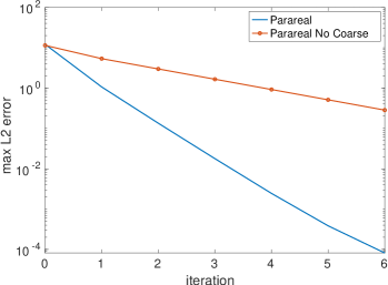
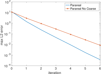
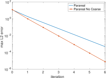
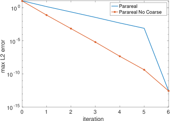
Figure 1: Running a classical Parareal algorithm with and without coarse propagator. From top left to bottom right: 48, 24, 12, and 6 coarse time intervals with $T=3$.

the results obtained with zero initial conditions, $u_{0}(x)=0$, and the source term

$$f(x,t)=10e^{-100(x-0.5)^{2}}\sum_{j=1}^{4}e^{-100(t-t_{j})^{2}},\quad t_{j}=0.1,0.6,1.35,1.85,$$ (5)

like a heating device which is turned on and of at specific time instances. We discretized the heat equation (4) using a centered finite difference discretization in space with mesh size $\Delta x=\frac{1}{128}$, and Backward Euler in time with time step $\Delta t=\frac{1}{96}$, and run the Parareal algorithm up to $T=3$ with various numbers $N$ of coarse time intervals, where the coarse propagator $G$ just does one big Backward Euler step. We see two really interesting results: first, the Parareal algorithm without coarse propagator is actually also converging when applied to the heat equation, both methods are a contraction. And second, if there are not many coarse time intervals, i.e. if the coarse time interval length $\Delta T$ is becoming large, the Parareal algorithm without coarse correction is converging even faster than with coarse correction!

In order to test this surprising property further, we repeat the above experiment, but use now homogeneous Neumann boundary conditions in (4), $\partial_{x}u(0,t)=\partial_{x}u(1,t)=0$, instead of the Dirichlet conditions. We show the corresponding results in Figure 2.

     

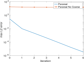
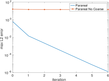
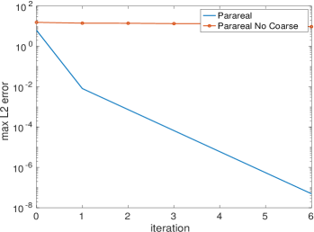
Figure 2: Classical Parareal with and without coarse propagator with zero Neumann boundary conditions. From top left to bottom right: 48, 24, 12, and 6 coarse time intervals and $T=3$.

We see that while the Parareal algorithm with coarse propagator is converging as before with Dirichlet conditions, the Parareal algorithm without coarse propagator is not converging any more, except in the last case when only 6 coarse time intervals are used, and here it is the finite step convergence property of the Parareal algorithm when iterating 6 times that leads to convergence, there is no contraction without the coarse propagator with Neumann boundary conditions.

It is very helpful at this point to take a closer look at the solutions we were computing in these two experiments for zero Dirichlet and zero Neumann conditions, shown in Figure 3 in the two leftmost panels.

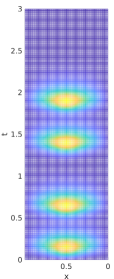
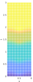
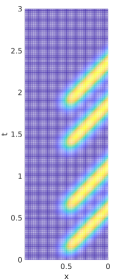
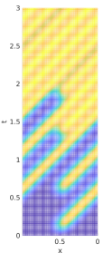
Figure 3: From left to right: solution of the heat equation model problem with zero Dirichlet and zero Neumann boundary conditions. Solution of the corresponding advection equation with Dirichlet boundary condition on the left and periodic boundary condition, and solution of the second order wave equation with zero Dirichlet boundary conditions.

We see that the solution with Dirichlet boundary conditions is very much local in time: in order to compute the solution around $t=2$, we only need to know if the right hand side function was on just before, but not at the much earlier times $t<<2$, since the solution does not contain this information any more. This is very different in the case of Neumann conditions, when using the same source term: now the solution at time $t=2$ strongly depends on the fact that the right hand side function was on at earlier times, since the heat injected into the system is kept, as a constant value in space. In analogy, it is very easy to predict the temperature in the room you are currently in a year from now, you only need to know if the heater or air-conditioner is on and the windows and doors are open or closed then, but not what happened with the room over the entire year before.

3 Convergence Analysis

In order to study our observation mathematically, it is easiest to consider a Parareal algorithm which uses a spectral method in space and is performing exact integrations in time for our heat equation model problem (4). The fine propagator $F(U_{n}^{k},T_{n},T_{n+1})$ is thus using a highly accurate spectral method in space with $m_{F}$ basis functions to solve (4), and the coarse propagator $G(U_{n}^{k},T_{n},T_{n+1})$ solves the same problem using a very cheap spectral method in space using only $m_{G}<<m_{F}$ basis functions. Note that we allow explicitly that $m_{G}=0$, which means the coarse solver is not present in the Parareal algorithm (1)!

A spectral representation of the solution of the heat equation (4) can be obtained using separation of variables, and considering a spatial domain $\Omega:=(0,\pi)$ to avoid to have to carry the constant $\pi$ in all the computations (see also Remark 3 later), we get

$$u(x,t):=\sum_{m=1}^{\infty}\hat{u}_{m}(t)\sin(mx).$$ (6)

Expanding also the right hand side in a sine series,

$$f(x,t):=\sum_{m=1}^{\infty}\hat{f}_{m}(t)\sin(mx),$$ (7)

and the initial condition,

$$u_{0}(x):=\sum_{m=1}^{\infty}\hat{u}_{0,m}(t)\sin(mx),$$ (8)

we find that the Fourier coefficients in the solution satisfy

$$\partial_{t}\hat{u}_{m}=-m^{2}\hat{u}_{m}+\hat{f}_{m},\quad\hat{u}_{m}(0)=\hat{u}_{0,m}.$$ (9)

The solution of this equation can be written in closed form using an integrating factor,

$$\hat{u}_{m}(t)=\hat{u}_{0,m}e^{-m^{2}t}+\int_{0}^{t}\hat{f}_{m}(\tau)e^{-m^{2}(t-\tau)}d\tau.$$ (10)

If we use in the Parareal algorithm (1) a spectral approximation of the solution for the fine propagator using $m_{F}$ modes, we obtain

$$F(U_{n}^{k},T_{n},T_{n+1})=\sum_{m=1}^{m_{F}}\left(\hat{U}_{m,n}^{k}e^{-m^{2}\Delta T}+\int_{T_{n}}^{T_{n+1}}\hat{f}_{m}(\tau)e^{-m^{2}(t-\tau)}d\tau\right)\sin(mx),$$ (11)

and similarly for the coarse approximation when using $m_{G}$ modes

$$G(U_{n}^{k},T_{n},T_{n+1})=\sum_{m=1}^{m_{G}}\left(\hat{U}_{m,n}^{k}e^{-m^{2}\Delta T}+\int_{T_{n}}^{T_{n+1}}\hat{f}_{m}(\tau)e^{-m^{2}(t-\tau)}d\tau\right)\sin(mx).$$ (12)

Because of the orthogonality of the sine functions, the Parareal algorithm (1) is diagonalized in this representation, which is the main reason that we chose a spectral method, to simplify the present analysis for this short note. For Fourier modes with $m\leq m_{G}$, the first and the third term in (1) coincide, as we see from (11) and (12), and thus cancel, and hence the Parareal update formula simplifies to

$$\begin{multlined}\hat{U}_{m,n+1}^{k+1}=\hat{U}_{m,n}^{k+1}e^{-m^{2}\Delta T}+\int_{T_{n}}^{T_{n+1}}\hat{f}_{m}(\tau)e^{-m^{2}(t-\tau)}d\tau,\\ ~{}\qquad\mbox{for $m=1,2,\ldots,m_{G}$.}\end{multlined}\hat{U}_{m,n+1}^{k+1}=\hat{U}_{m,n}^{k+1}e^{-m^{2}\Delta T}+\int_{T_{n}}^{T_{n+1}}\hat{f}_{m}(\tau)e^{-m^{2}(t-\tau)}d\tau,\\ ~{}\qquad\mbox{for $m=1,2,\ldots,m_{G}$.}$$ (13)

For $m>m_{G}$, the coarse correction term is not present in the Parareal update formula (1), and thus only the contribution from the fine propagator remains,

$$\begin{multlined}\hat{U}_{m,n+1}^{k+1}\!=\!\hat{U}_{m,n}^{k}e^{-m^{2}\Delta T}\!+\!\int_{T_{n}}^{T_{n+1}}\!\!\!\hat{f}_{m}(\tau)e^{-m^{2}(t-\tau)}d\tau,\\ \mbox{for $m=m_{G}+1,m_{G}+2,\ldots,m_{F}$.}\end{multlined}\hat{U}_{m,n+1}^{k+1}\!=\!\hat{U}_{m,n}^{k}e^{-m^{2}\Delta T}\!+\!\int_{T_{n}}^{T_{n+1}}\!\!\!\hat{f}_{m}(\tau)e^{-m^{2}(t-\tau)}d\tau,\\ \mbox{for $m=m_{G}+1,m_{G}+2,\ldots,m_{F}$.}$$ (14)

The only difference is the iteration index $k$ in the first term on the right, but this term makes all the difference: for $m\leq m_{G}$, the update formula (13) represent the exact integration of the corresponding mode sequentially going through the entire time domain $(0,T)$. For $m>m_{G}$, the update formula (14) represents simply a block Jacobi iteration solving all time subintervals $(T_{n},T_{n+1})$ in parallel starting from the current approximation at iteration $k$. Using this insight, we obtain the following convergence result.

Theorem 1 (Parareal convergenve even without coarse propagator).

The Parareal algorithm (1) for the heat equation (4) using the spectral coarse propagator (12) and the spectral fine propagator (11) satisfies for any initial guess $U_{n}^{0}$ the convergence estimate

$$\sup_{n}||U_{n}^{k}(\cdot)-u(\cdot,T_{n})||_{2}\leq e^{-(m_{g}+1)^{2}k\Delta T}\sup_{n}||U_{n}^{0}(\cdot)-u(\cdot,T_{n})||_{2},$$ (15)

and this estimate also holds if the coarse propagator does not contain any modes, $m_{G}=0$, which means it is not present. The Parareal algorithm therefore converges also without coarse propagator.

Proof.

We introduce the error in Fourier space at the interfaces, $\hat{E}_{m,n}^{k}:=\hat{U}_{m,n}-\hat{U}_{m,n}^{k}$, where the converged solution $\hat{U}_{m,n}$ satisfies

$$\hat{U}_{m,n+1}=\hat{U}_{m,n}e^{-m^{2}\Delta T}+\int_{T_{n}}^{T_{n+1}}\hat{f}_{m}(\tau)e^{-m^{2}(t-\tau)}d\tau,\quad\mbox{for all $m=1,2,\ldots$.}$$ (16)

Taking the difference with the Parareal update formula for small $m$ in (13) and using the fact that $U_{m,0}^{k}=U_{m,0}=u^{0}$, we thus obtain a vanishing error in the first Fourier coefficients after having performed one Parareal iteration,

$$\hat{E}_{m,n}^{k}=0,\quad m=1,2,\ldots,m_{G},\quad k=1,2,\ldots.$$

For $m>m_{G}$, taking the difference between (16) and the update formula for larger $m$ in (14), the part with the source term $f$ cancels, and we are left with

$$\hat{E}_{m,n}^{k+1}=\hat{E}_{m,n}^{k}e^{-m^{2}\Delta T},\quad m=m_{G}+1,m_{G}+2,\ldots.$$

Now using the Parseval-Plancherel identity, and taking the largest convergence factor $e^{-(m_{G}+1)^{2}\Delta T}$ out of the sum, we obtain the convergence estimate (15) taking the sup over all time intervals $n$. ∎

We show in Figure 4 a graphical comparison of the convergence factor of each Fourier mode without coarse propagator from (15), i.e. $e^{-m^{2}\Delta T}$, and with coarse propagator $\frac{|e^{-m^{2}\Delta T}-R_{G}(-m^{2}\Delta T)|}{1-|R_{G}(-m^{2}\Delta T)|}$ from [8] for one Backward Euler step, $R_{G}(z)=\frac{1}{1-z}$, as we used for Figures 1 and 2.

\begin{overpic}[width=195.12767pt,trim=90.3375pt 260.97499pt 100.37498pt 130.48749pt,clip]{PararealNoCoarseComparison1.pdf} \put(32.8,2.5){$m$} \put(74.3,1.7){$\Delta T$} \end{overpic} \begin{overpic}[width=216.81pt,trim=62.2325pt 364.36124pt 94.3525pt 55.20624pt,clip]{PararealNoCoarseComparison3.pdf} \put(51.5,8.5){\small$m$} \end{overpic}

Figure 4: Contraction for each Fourier mode $m$ as function of the Parareal time interval length $\Delta T$ with (blue, PdT=$\Delta T$) and without (green, PNCdT=$\Delta T$) coarse propagator.

We see that indeed there are situations where the coarse correction with one Backward Euler step is detrimental, as observed in Figures 1 and 2, and there is also quantitative agreement.

Remark 1.

Theorem 1 shows that the Parareal algorithm (1) for the heat equation is scalable, provided the time interval length $\Delta T$ is held constant: no matter how many such time intervals are solved simultaneously, the convergence rate remains the same, and this even in the case without coarse propagator! This is like the scalability of one level Schwarz methods discovered in [1] for molecular simulations in solvent models, and rigorously proved in [2, 3, 4] using three different techniques: Fourier analysis, maximum principle, and projection arguments in Hilbert spaces.

Remark 2.

If we had zero Neumann boundary conditions, a similar result could also be derived using a cosine expansion, but then no coarse correction would not lead to a convergent method, since the zero mode would have the contraction factor one. One must therefore in this case have at least the constant mode in the coarse correction for the Parareal algorithm to converge. Otherwise however all remains the same.

Remark 3.

A precise dependence on the domain size can be obtained by introducing the spatial domain of length $L$, $\Omega=(0,L)$. In this case the convergence factor simply becomes $e^{-\left(\frac{(m_{G}+1)\pi}{L}\right)^{2}\Delta T}$. The same estimate can also be obtained for a more general parabolic equation, the convergence factor then becomes $e^{-\lambda_{m_{G}+1}\Delta T}$, where $\lambda_{m_{G}+1}$ is the $m_{G}$ plus first eigenvalue of the corresponding spatial operator.

4 Conclusions

We have shown that Parareal without a coarse propagator can converge very well for the prototype parabolic problem of the heat equation, because such problems “forget” all fine information over time, and only very coarse information, if at all, remains, depending on the boundary conditions. This is very different for hyperbolic problems: while for the advection equation $u_{t}+au_{x}=f$ with Dirichlet boundary condition, whose solution is shown in Figure 3 (middle) the information is also “forgotten” by leaving the domain on the right and Parareal converges very well [5], also without coarse propagator, for the advection equation with periodic boundary conditions in the fourth plot of Figure 3 this is not the case any more: nothing is forgotten, and the coarse propagator needs to have fine accuracy quality for the Parareal algorithm not to fail. The situation is similar for the second order wave equation $u_{tt}=u_{xx}$, whose solution is shown on the right in Figure 3.

Acknowledgement.

Funded by the Deutsche Forschungsgemeinschaft (DFG, German Research Foundation) under Germany’s Excellence Strategy EXC 2044 – 390685587, Mathematics Münster: Dynamics–Geometry–Structure and the Swiss National Science Foundation.

References

- [1] Eric Cances, Yvon Maday, and Benjamin Stamm. Domain decomposition for implicit solvation models. The Journal of chemical physics, 139(5), 2013.
- [2] Gabriele Ciaramella and Martin J. Gander. Analysis of the parallel Schwarz method for growing chains of fixed-sized subdomains: Part I. SIAM Journal on Numerical Analysis, 55(3):1330–1356, 2017.
- [3] Gabriele Ciaramella and Martin J. Gander. Analysis of the parallel Schwarz method for growing chains of fixed-sized subdomains: Part II. SIAM Journal on Numerical Analysis, 56(3):1498–1524, 2018.
- [4] Gabriele Ciaramella and Martin J. Gander. Analysis of the parallel Schwarz method for growing chains of fixed-sized subdomains: Part III. Electron. Trans. Numer. Anal, 49:201–243, 2018.
- [5] Martin J. Gander. Analysis of the parareal algorithm applied to hyperbolic problems using characteristics. SeMA Journal: Boletín de la Sociedad Española de Matemática Aplicada, (42):21–36, 2008.
- [6] Martin J. Gander and Ernst Hairer. Nonlinear convergence analysis for the parareal algorithm. In Domain decomposition methods in science and engineering XVII, pages 45–56. Springer, 2008.
- [7] Martin J. Gander and Ernst Hairer. Analysis for parareal algorithms applied to hamiltonian differential equations. Journal of Computational and Applied Mathematics, 259:2–13, 2014.
- [8] Martin J. Gander and Stefan Vandewalle. Analysis of the parareal time-parallel time-integration method. SIAM Journal on Scientific Computing, 29(2):556–578, 2007.
- [9] Jacques-Louis Lions, Yvon Maday, and Gabriel Turinici. Résolution d’edp par un schéma en temps pararéel. Comptes Rendus de l’Académie des Sciences-Series I-Mathematics, 332(7):661–668, 2001.
- [10] Toshiya Takami and Daiki Fukudome. An identity parareal method for temporal parallel computations. In Parallel Processing and Applied Mathematics: 10th International Conference, PPAM 2013, Warsaw, Poland, September 8-11, 2013, Revised Selected Papers, Part I 10, pages 67–75. Springer, 2014.