Precise asymptotics of the spin Teukolsky field in the Kerr black hole interior
Abstract.
Using a purely physical-space analysis, we prove the precise oscillatory blow-up asymptotics of the spin Teukolsky field in the interior of a subextremal Kerr black hole. In particular, this work gives a new proof of the blueshift instability of the Kerr Cauchy horizon against linearized gravitational perturbations that was first shown by Sbierski [38]. In that sense, this work supports the Strong Cosmic Censorship conjecture in Kerr spacetimes. The proof is an extension to the Teukolsky equation of the work [26] by Ma and Zhang that treats the scalar wave equation in the interior of Kerr. The analysis relies on the generic polynomial decay on the event horizon of solutions of the Teukolsky equation that arise from compactly supported initial data, as recently proved by Ma and Zhang [27] and Millet [30] in subextremal Kerr.
1. Introduction
1.1. The Kerr black hole interior
We begin with a review of the main features of the interior of Kerr black holes. The Kerr metric describes the spacetime around and inside a rotating non-charged black hole. It is a two-parameter family of stationary and axisymmetric solutions of the Einstein vacuum equations that write, denoting the Ricci tensor associated to a Lorentzian metric ,
| (1.1) |
The two parameters are the mass and the angular momentum per unit mass of the black hole. In this work, we only consider subextremal Kerr with non-zero angular momentum, i.e. such that . The Kerr metric is given in Boyer-Lindquist coordinates by
where , , . We define
where are the roots of . The singularities of the metric are coordinate singularities that vanish when considering Eddington-Finkelstein coordinates
where , , see Section 2.1. The event horizon and the Cauchy horizon can then be properly attached to the Lorentzian manifold equipped with the metric , see [31, Chapter 2] for more details. We will mainly be interested in a region containing the right event horizon and the right Cauchy horizon that are respectively defined by
Note that a result similar to our main theorem can be deduced in a region containing the left event and Cauchy horizons, that are defined by
We denote and the bifurcations spheres, and , (resp. , ) the right (resp. left) timelike and null infinities.
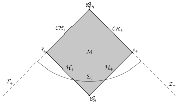
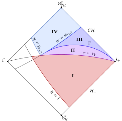
In this work, by ’Kerr interior’ we mean the resulting Lorentzian manifold which is to which we attach its boundaries, the event and Cauchy horizons. We will be interested in the asymptotics at of solutions to the Teukolsky equation, that arise from compactly supported initial data on a spacelike hypersurface . See Figure 1 for the Penrose diagram of Kerr interior and an illustration of the hypersurface .
1.2. Teukolsky equations
Teukolsky [42] found that, when linearising a gravitational perturbation of a Kerr black hole in the Newman-Penrose formalism, two curvature components decouple from the linearised gravity system and satisfy wave equations, called the Teukolsky equations. More precisely, we first define the pair of null vector fields given in Boyer-Lindquist coordinates by
which is aligned with the principal null directions of the Kerr spacetime, and which is regular on . We then define the rescaled null pair
which is regular on . We also define the slightly modified null pair
and the complex vector field
Then, denoting the linearized curvature tensor, the scalars
are called respectively the spin and spin Teukolsky scalars. They satisfy the Teukolsky equations that write, for ,
| (1.2) |
The rescaled scalars
satisfy a rescaled version of the Teukolsky equation, see Section 2.4.1 for the precise definition of the Teukolsky wave operators. Notice that and are projections of the linearized curvature on a frame that is regular on , while , are projections of the linearized curvature on a frame that is regular on . Thus the main result of this work, namely the blow-up asymptotics of at , is a linear curvature instability statement for the Kerr Cauchy horizon.
The Teukolsky equations were originally introduced to study the stability of the exterior of Kerr black holes. For a review of the litterature concerning the Teukolsky equations, see the introduction of [16], where the decay estimates for the nonlinear analog of the Teukolsky equations derived in [16] are used to prove the nonlinear stability of the exterior of slowly rotating Kerr black holes in [19].
1.3. Blueshift effect and Strong Cosmic Censorship conjecture
1.3.1. Blueshift effect
The Kerr spacetime is globally hyperbolic only up to the Cauchy horizon . Thus the part of the spacetime that is beyond the Cauchy horizon, in the region , can be thought as unphysical as it is not determined by the data on any spacelike hypersurface inside . In other words, the Kerr spacetime can be extended across the Cauchy horizon as a regular solution of the Einstein vacuum equations (1.1) in infinitely many ways, which goes against determinism in general relativity.
However, it is expected that this unphysical feature is just an artefact of the ideal Kerr spacetime. Indeed, realistic astrophysical black holes are perturbations of Kerr, i.e. they are the maximal globally hyperbolic developpement of initial data close to the one of Kerr. It is expected that these perturbations kill the non-physical features of ideal Kerr. In the linear setting, this is the so-called blueshift effect, introduced by Simpson and Penrose in 1972 [40]. It is a heuristic argument according to which the geometry of Kerr interior (they initially wrote the argument for Reissner–Nordström) forces propagating waves to blow-up in some way at the Cauchy horizon. This effect is illustrated on Figure 2, and is linked to the Strong Cosmic Censorship conjecture.
1.3.2. Strong Cosmic Censorship conjecture
The Strong Cosmic Censorship (SCC) conjecture was formulated by Penrose in [34], and, in its rough version, states the following :
Conjecture 1.1 (Strong Cosmic Censorship conjecture, rough version).
The maximal globally hyperbolic developpement (MGHD) of generic initial data for the Einstein equations is inextendible.
In other words, this conjecture states that the unphysical, non-deterministic behavior of spacetimes with non-empty Cauchy horizons (for example Kerr and Reissner-Nordström spacetimes) is non-generic, and thus vanishes upon small perturbations. See [5, 6] for more modern versions of the SCC conjecture.
A fundamental question in SCC is the regularity for which the MGHD of initial data should be inextendible. The formulation of SCC was disproved in Kerr by Dafermos and Luk [11]. They showed that generic perturbations of the interior of Kerr still present a Cauchy horizon across which the metric is continuously extendible. They also argued that the perturbed Cauchy horizon may be a so-called weak null singularity, which is a singularity weaker than a spacelike curvature singularity as in Schwarzschild. For references on weak null singularities, see [20], [46]. See [39] for a link between weak null singularities and the formulation of SCC.
In spherical symmetry, the instability of the Cauchy horizon for the model of the Einstein-Maxwell-scalar field system was proven in [22] and [23], extending the results of [9]. See also [44, 45] for analog results for the Einstein-Maxwell-Klein-Gordon equations. In Kerr, which is only axisymmetric, the full nonlinear problem for the Einstein equations is still open, and we focus in this paper on the model of linearized gravity, where the Teukolsky scalar represents a specific component of the perturbed curvature tensor. Our main result, namely the blow-up of on , thus supports the SCC conjecture in the linearized setting.
1.4. Black hole interior perturbations
1.4.1. Results related to Price’s law
The starting point to prove the instability of solutions of the Teukolsky equation in Kerr interior is Price’s law for Teukolsky, i.e. the polynomial lower bound on the event horizon for solutions of the Teukolsky equation arising from compactly supported initial data, see [17, 35, 36, 37] for the original works on Price’s law. A version of Price’s law for the Teukolsky equations in Kerr was heuristically found by Barack and Ori in [3].
In this paper we use the precise Price’s law asymptotics on given by Ma and Zhang in [27] for the Teukolsky equations111The Price’s law in [27] holds for , and for conditionally on an energy-Morawetz bound. This energy-Morawetz estimate has since been proved for by Teixeira da Costa and Shlapentokh-Rothman in [7, 8], so that the Price’s law in [27] holds for the full range .. For another proof of the polynomial lower bound in the full subextremal range for solutions of the Teukolsky equation, see the work of Millet [30], that uses spectral methods. For a complete account of results related to Price’s law, see [27].
1.4.2. Previous results on black hole interior perturbations
The first works on the linear instability of the Cauchy horizons in Kerr and Reissner-Nordström black holes consisted in finding explicit solutions that become unbounded in some way at the Cauchy horizon, see for example [28]. In [33], a heuristic power tail asymptotic for scalar waves in the interior of Kerr black holes was obtained. Regarding the Teukolsky equations, the oscillatory blow-up asymptotic of our main result in the interior of Kerr black holes, see (1.3), was first predicted heuristically by Ori [32], writing the azimuthal -mode of the solution as a late-time expansion ansatz of the form
The asymptotic behavior (1.3) was also confirmed in a numerical simulation [4].
A rigorous boundedness statement for solutions of the scalar wave equation inside the spherically symmetric Reissner-Nordström spacetime was proven in [14]. Still for the scalar wave equation in the interior of Reissner-Nordström black holes, the blow-up of the energy of generic scalar waves was obtained in [21]. A scattering approach to Cauchy horizon instability in Reissner-Nordström, as well as an application to mass inflation, was presented in [24], on top of the non-linear instability results [22, 23, 9, 44, 45] already mentionned in Section 1.3.2.
In Kerr, for the scalar wave equation, a generic blow-up result for the energy of solutions on the Cauchy horizon was obtained in [25], while the boundedness of solutions at the Cauchy horizon was proven in [18] in the slowly rotating case. The boundedness result was then extended to the full subextremal range in [13]. A construction of solutions that remain bounded but have infinite energy at the Cauchy horizon was presented in [12]. Finally, the precise asymptotics of the scalar field in the interior of a Kerr black hole was proven in [26] using a purely physical-space analysis.
Concerning the Teukolsky equations in Kerr interior, the method of proof of [25] was extended to the spin Teukolsky equation in the work [38], that proved the blow-up of a weighted norm on a hypersurface transverse to the Cauchy horizon, relying on frequency analysis.
The goal of the present paper is to rigorously prove the oscillatory blow-up asymptotics of the spin Teukolsky field in the Kerr black hole interior, by extending the physical-space approach of [26] to Teukolsky equations, thus providing a new proof of the blow-up results of [38].
We discussed here the references on black hole interior perturbations that are the most relevant to this work. For a more complete account of the results related to black hole interior perturbations, for example in Schwarschild interior or in the cosmological setting, see the introduction in [38].
1.5. Rough version of the main theorem
This paper rigorously proves the blueshift instability on the Kerr Cauchy horizon for solutions of the spin Teukolsky equations, by finding the precise oscillatory blow-up asymptotics of the spin Teukolsky scalar. The rough version of the main result of this paper is the following, see Theorem 3.2 for the precise formulation.
Theorem 1.2 (Main theorem, rough version).
Assume that the Price’s law polynomial lower bounds on the event horizon for solutions of the Teukolsky equations hold, as proven in [27, 30]. Denote the spin Teukolsky scalar obtained in a principal null frame regular on the Cauchy horizon. Then blows up at the Cauchy horizon, exponentially in the Eddington-Finkelstein coordinate , and oscillates at a frequency that blows up at the Cauchy horizon. More precisely,
-
(1)
the amplitude is proportionnal to ,
-
(2)
the oscillation frequency blows-up like .
Remark 1.3.
We remark the following :
-
•
Anticipating some of the notations that will be introduced later on, we actually show the following precise asymptotic behavior near :
(1.3) where the constants depend on the initial data on and are generically non-zero, the constants are non-zero for (see Remark 3.3), is an angular coordinate that is regular on , the functions are the spin-weighted spherical harmonics, and near , see Sections 2.1 and 2.2 for more details.
-
•
The blueshift instability at for was first proven recently by Sbierski [38] who showed the blow-up of a weighted norm along a hypersurface transverse to . This result suggests a blow-up that is exponential in the Eddington-Finkelstein coordinate , the Cauchy horizon corresponding to . We prove in this paper a pointwise exponential blow-up, along with an oscillatory behavior, which were both heuristically predicted by Ori [32].
- •
1.6. Structure of the proof
Although our main result will be about the precise asymptotics of at , we will actually also obtain precise estimates for near , and we will use the Teukolsky-Starobinsky identities (see Section 2.4.2) to link and there.
For , we denote the differential operator on the left-hand side of (1.2), called the Teukolsky operator, and the rescaled Teukolsky operator, such that
The analysis is done entirely in physical space, using energy estimates to prove upper bounds on ’error’ quantities, in the hope that this method of proof is robust enough to be applied in a more general setting. The first step is to notice that the energy estimates to get polynomial upper bounds done in [26] for the scalar wave equation in the Kerr interior can be extended to the Teukolsky equations , but only for negative spin close to , and for positive spin close to . This is because we need a fixed sign for the scalar that appears at crucial places in the energy estimates, where is the spin, and because while .
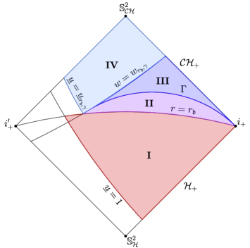
We denote the region containing , and the regions close to where has exponential decay in , and the intermediate region between and . See Figure 3 and Section 3.1 for the precise definitions of the regions. The assumptions on that we will use are the ones given by [27], i.e. that the error quantities
| (1.4) | ||||
| (1.5) |
are bounded by on where , see Sections 2.1 and 3.2 for the definitions of , , , . The main steps of the proof then go as follows :
-
(1)
First, we propagate Price’s law lower bound for in . To do this, we propagate the upper bound of from to using a redshift energy estimate. This is only possible in region that contains the event horizon.
-
(2)
We then use the Teukolsky-Starobinsky identity (2.34) to propagate in the Price’s law upper bound on for .
-
(3)
Next, similarly as in we propagate the lower bound for in using an effective blueshift energy estimate for , which is only possible for close to . This step in region is necessary to propagate the lower bound up to where the analysis becomes more delicate (namely, where we can’t anymore get sharp decay of the energy from an energy estimate because of the geometry of the Kerr black hole interior near the Cauchy horizon).
-
(4)
We then obtain a non-sharp bound for in using an energy estimate.
-
(5)
To get the blow-up asymptotics in , we rewrite the Teukolsky equation as a wave equation
(1.6) where we use the previous bound to control the right-hand-side. This is where we can effectively see the blueshift heuristic in action. The geometry of Kerr interior is such that is regular on , and reporting that in the Teukolsky equation gives a factor on the source term that becomes negligeable in . Integrating (1.6) from directly gives the announced blow-up asymptotics for . This is where we use the definition of region : decays exponentially in in , which easily bounds the error terms.
-
(6)
We cannot integrate the wave equation in because the slices starting inside do not cross . Instead, commuting and the Teukolsky operator, we estimate in , which allows us to propagate the blow-up of from to by integration.
Remark 1.4.
Here are some further remarks on the analysis :
-
•
To control the derivatives of the error terms, we commute the Teukolsky equation with operators that have good commutations properties, namely , , , and the Carter operator.
-
•
Note that, at any point in the analysis, in any region , , , , any estimate that we get can be turned into an estimate in the symmetric region by replacing with , with , with and with . As in [26], this will be useful in region .
Remark 1.5.
Here are some differences from the previous works in the method of proof :
-
•
Our physical-space proof differs substantially from [38] that relies in a crucial way on frequency analysis.
-
•
In [26] for the scalar wave equation, the proof is made by decomposing the scalar field onto its and modes : . Using the decay of both quantities on the event horizon, it is shown, commuting the wave equation with the projection on the modes, that the lower bound for and the better decay of propagate. This is different from our proof, where there is no projection on the (spin-weighted) spherical harmonics. We do not need to assume that the modes of decay better than on . Moreover, in the blueshift region (i.e. for close to ) we will use easier estimates than [26] that introduces multipliers, taking advantage of the fact that we deal with a non-zero spin.
1.7. Overview of the paper
In Section 2, we introduce the geometric background, the operators, the coordinates that we will use in the analysis, as well as the system of equations that we consider. In Section 3, we recall the decay assumptions on the event horizon, the so-called Price’s law, and we write the precise version of the main theorem. In Section 4, we obtain the redshift energy estimates in for and use the Teukolsky-Starobinsky identity to get the lower bound for in . Section 5 deals with the effective blueshift energy estimates to propagate the lower bound for in . In Section 6, we get the non-sharp bound for in and we compute and integrate the wave equation that will eventually give the precise oscillatory blow-up asymptotics for in , before propagating this blow-up to region .
1.8. Acknowledgments
The author would like to thank Jérémie Szeftel for his support and many helpful discussions, and Siyuan Ma for helpful suggestions. This work was partially supported by ERC-2023 AdG 101141855 BlaHSt.
2. Preliminaries
We first introduce some notations. By ’LHS’ and ’RHS’ we mean respectively ’left-hand side’ and ’right-hand side’. If is an operator acting on a (spin-weighted) scalar , for an integer and for any norm , we use the notation
If are two non-negative scalars, we write whenever there is a constant that depends only on the black hole parameters , on the initial data, and on the smallness constants , , such that on the region considered. We write when . We write when and .
2.1. Geometry of the interior of subextremal Kerr spacetimes
First, we fix a notation for the Boyer-Lindquist (B-L) coordinate Killing vector fields :
Note that when we write , , we mean the B-L coordinate vector fields. We recall the definition of the null pair that we use :
| (2.1) |
This pair satisfies
and is regular on , as can be seen by expressing and with the ingoing Eddington-Finkelstein coordinate vector fields, see below. We also define the rescaled null pair
| (2.2) |
that is regular on .
As recalled in the introduction, the B-L coordinates are not adapted to the geometry of Kerr, because they are singular at both the event and Cauchy horizons. In this paper, we will use both the Eddington-Finkelstein coordinates and double null-like coordinates (we borrow the terminology from [26]) introduced in Section 2.1.3. Notice that the scalar function
vanishes only on the horizons, and that unlike in the Kerr black hole exterior region, on . Define the tortoise coordinate by
Notice that as and as . More precisely, defining and the surface gravities of the event and Cauchy horizons :
then the asymptotics of at the horizons are given by
| (2.3) |
where has a finite limit as . Notice that (2.3) implies that, for close to ,
while for close to ,
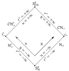
Next, we define the coordinates
The range of the coordinates is indicated on Figure 4. Recall that the right event horizon corresponds to , while the right Cauchy horizon corresponds to .
As in [26], define also the function such that
Then define the ingoing and outgoing angular coordinates
The coordinates and are regular on and , while and are regular on and .
2.1.1. Ingoing Eddington-Finkelstein coordinates
The ingoing Eddington-Finkelstein coordinates are . It is a set of coordinates that is regular on and . The coordinate vector fields are
| (2.4) |
2.1.2. Outgoing Eddington-Finkelstein coordinates
The outgoing Eddington-Finkelstein coordinates are . It is a set of coordinates that is regular on and . The coordinate vector fields are
| (2.5) |
2.1.3. Double null-like coordinate systems
As in [26], we also use the ingoing double null-like coordinates that are regular at (where ), with coordinate vector fields
| (2.6) |
where we denote the B-L coordinate vector field to avoid confusion. The equivalent outgoing double null-like coordinates are regular at (where ), with coordinate vector fields
| (2.7) |
Note that we will only use the ingoing double null-like coordinate system in the redshift region , and the outgoing double null-like coordinate system in the blueshift region so we use the same notations for the ingoing and outgoing double null-like coordinate vector fields , , as there is no danger of confusion.
2.1.4. Constant and spacelike hypersurfaces
We need a family of spacelike hypersurfaces, for which we will apply the energy estimates and get decay in . Note that the constant hypersurfaces are not spacelike. Indeed we have
so that the constant hypersurfaces are null at the poles and timelike away from the poles. We define, as in [26],
such that the constant and hypersurfaces are spacelike. Indeed, we have [26]
2.2. Spin-weighted scalars
2.2.1. Spin-weighted scalars and spin-weighted spherical operators
In this section, we consider the round sphere equipped with its volume element, written in coordinates :
Let be an integer. Note that in this work we only consider . A spin scalar is a scalar function that has zero boost weight and proper spin weight, as defined by Geroch, Held and Penrose [15]. See [38] for a rigorous presentation of the spaces of spin-weighted scalars on the sphere and on the Kerr interior, and a proof that the Teukosky scalar obtained in the linearisation of a gravitational perturbation in the Newman-Penrose formalism is a spin-weighted scalar on spacetime. See also [29] for a precise review of the geometric background of the Teukolsky equation. By ’spin-weighted operator’ we mean an operator that takes a spin-weighted scalar into a spin-weighted scalar. Note that a spin scalar is a scalar function.
In Kerr spacetime, the volume element induced on the topological spheres
by the metric is
where in the Kerr interior. Thus, although they are not round, we still rely on the round volume element on the Kerr spheres to define norms.
Definition 2.1.
For a spin-weighted scalar on , we define
Notice that on a region with , in the ingoing Eddington-Finkelstein coordinates, as is constant on , the definition of the norm gives
which is a regular norm up to the event horizon . For the same reason, on a region with , we have
which is a regular norm up to the Cauchy horizon .
Definition 2.2.
We recall the definition of the following standard spin-weighted differential operators, called the spherical eth operators :
| (2.8) | ||||
| (2.9) |
Remark 2.3.
The spherical eth operators modify the spin when applied to a spin-weighted scalar. More precisely, increases the spin by while decreases the spin by . See in Section 2.2.2 their effect on spin-weighted spherical harmonics. Note that the spin of the scalar to which we apply the eth operators will be clear in the context, so we drop the subscript in what follows.
Definition 2.4.
We define the spin-weighted Laplacian as
| (2.10) |
Remark 2.5.
We also have the expression
| (2.11) |
2.2.2. Spin-weighted spherical harmonics
Let be a fixed spin. The spin-weighted spherical harmonics are the eigenfunctions of the spin-weighted Laplacian, that is self-adjoint on . They are given by the following family
of spin scalars on the sphere . They form a complete orthonormal basis of the space of spin scalars on , for the scalar product. When considering the spheres of Kerr interior, as the B-L coordinate is singular at the horizons, we need a slightly modified family. Let . Then for such that , the spin scalars
form a complete orthonormal basis of the space of spin scalars on , for the scalar product. Similarly, if , the spin scalars
form a complete orthonormal basis of the space of spin scalars on , for the scalar product.
Remark 2.6.
In this work, we will never project equations or spin-weighted scalars on some or modes, unlike in [26] and [27]. Instead, we will simply propagate the dominant term of on up to . This dominant term is a linear combination of spin-weighted spherical harmonics, and satisfies key properties (see Proposition 5.7) that rely on their algebraic properties.
The following facts are standards. We have :
| (2.12) | ||||
| (2.13) | ||||
| (2.14) | ||||
| (2.15) |
2.3. Functional inequalities
We start this section by recalling [26, Lemma 3.4] with , which will be used to deduce decay of the energy from an energy estimate.
Lemma 2.7.
Let and let be a continuous function. Assume that there are constants , such that for ,
Then for any ,
where is a constant that depends only on , and .
Proof.
See [26, Lemma 3.4]. ∎
2.3.1. and spin-weighted operators in Kerr spacetime
Definition 2.8.
We define the spin-weighted Carter operator
| (2.16) |
The main property of the spin-weighted Carter operator is that it commutes with the Teukolsky operator (see (2.30), (2.31)). We will use it to bound the angular derivates of solutions to the Teukolsky equation. The following operator is (up to a bounded potential) the spin-weighted scalar equivalent of the tensor covariant derivative , where
and will be useful to get a Poincaré-type inequality to absorb the zero order terms of the Teukolsky operator when doing energy estimates.
Definition 2.9.
We define the spin-weighted operator
| (2.17) |
Note that is not regular at the poles, but for a spin-weighted scalar on spacetime we still have , see for example [38, Eq. (2.34)]. We will need the following integration by parts lemma for .
Lemma 2.10.
Let , be spin scalars on . Then
Proof.
Define the real valued function
We have
as stated. ∎
Remark 2.11.
Notice that we have the expression
| (2.18) | ||||
| (2.19) |
In particular, , and .
2.3.2. Poincaré and Sobolev inequalities for spin-weighted scalars
We first recall the standard Poincaré inequality for spin-weighted scalars, see for example [10, Eq. (34)].
Proposition 2.12.
Let be a spin scalar on . Then
| (2.20) |
Next, we define the energy for wich we will show decay for solutions of the Teukolsky equation.
Definition 2.13.
Let be a spin-weighted scalar on . We define its energy density and degenerate energy density as the scalars
| (2.21) | ||||
| (2.22) |
The following result is a re-writing of the standard Poincaré inequality (2.20), that will be useful in the energy estimates.
Proposition 2.14.
Let be a spin scalar on . For any we have the Poincaré inequality
| (2.23) |
Proof.
We now recall the standard Sobolev embedding for spin-weighted scalars, see for example Lemma 4.27 and Lemma 4.24 of [2].
Proposition 2.15.
Let be a spin scalar on . We have
| (2.25) |
We will need the following reformulation of the standard Sobolev embedding :
Proposition 2.16.
Let be a spin scalar on . For any we have
| (2.26) |
2.4. System of equations
2.4.1. Different expressions of the Teukolsky operators
Recall from (1.2) the expression of the Teukolsky operator obtained in a frame regular at , originally found by Teukolsky [42] :
such that for , the spin Teukolsky equation writes
The rescaled Teukolsky operator, obtained in the rescaled frame that is regular on is
such that for , recalling ,
The expression of in B-L coordinates is
Notice that
| (2.27) |
To do the energy estimates, it is convenient to write the Teukolsky operators in terms of , , and .
Proposition 2.17.
We have :
| (2.28) |
| (2.29) |
Proof.
The Teukolsky operators can also be written [27, (3.3)] as
| (2.30) | |||
| (2.31) |
Note that these expressions show the crucial fact that , and the Carter operator commute with the Teukolsky equation :
| (2.32) |
To compute the commutator of the Teukolsky operator with , we will rewrite in terms of , , and the angular operators.
Proposition 2.18.
We have
Proof.
Proposition 2.19.
We have
Proof.
We simply use the above expression for and the fact that . ∎
2.4.2. Teukolsky-Starobinsky identities
On top of the Teukolsky equations, we also assume that the Teukolsky-Starobinsky identities (TSI) hold. The Teukolsky-Starobinsky identities are a PDE system relating the 4th order angular and radial derivatives of . Like the Teukolsky equations, they are obtained from the linearisation of a gravitational perturbation of the Einstein vacuum equations around Kerr spacetime. Their differential form was first derived in [41, 43] in frequency space, while their covariant form is derived in [1]. Recalling from (2.4), (2.5) the coordinate vector fields
the TSI for the spin write [27, Lemma 3.21], in Kerr spacetime,
| (2.33) | ||||
| (2.34) |
As mentionned in [27], (2.33) and (2.34) are physical space versions of the frequency space TSI’s obtained in [41, 43], and it is also possible to obtain (2.33) and (2.34) from the covariant TSI in [1]. We will actually only use (2.34) in this work, close to , and not (2.33).
3. Statement of the main theorem
Recall that we denote by , the spin and scalars that are solutions of the spin Teukolsky equations :
| (3.1) |
As before, we denote that satisfies . In this section, we state our main result on the precise asymptotics of at . To this end, we first introduce the different subregions of the Kerr interior that we will consider.
3.1. The different regions of the Kerr black hole interior
Fix close to , small, that will both be chosen later in the energy estimates. More precisely, is chosen in Appendix A.3 and is chosen in Section 5.1. We define the following subregions of the Kerr black hole interior, see Figure 6 :
where and are such that and intersect and , where the hypersurface is defined by
Region is the redshift region that contains , region is the blueshift region very close to where the scalar decays exponentially towards the Cauchy horizon, and region is an intermediate region, where the blueshift effect is already effective.
In region we will obtain redshift energy estimates for the Teukolsky equation for , while in we will derive effective blueshift estimates for . For the energy estimates, we use the coordinate system in , and the coordinate system in .
In the next section, we provide the assumptions on on which all the analysis is based. The goal of the analysis will be to successively propagate the polynomial bounds on to regions , , and .
3.2. Main assumptions on the event horizon
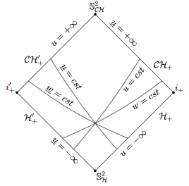
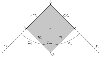
We first define our initial spacelike hypersurface as the union of three spacelike hypersurfaces :
similarly as in [26]. More precisely, we define as the hypersurface defined in [27], i.e. a constant hypersurface, where is a hyperboloidal coordinate system on the right part of the exterior of Kerr spacetime. Similarly, is a constant hypersurface, where is a hyperboloidal coordinate system on the left part of the exterior of Kerr spacetime. We chose as any spacelike hypersurface inside the Kerr interior that joins and such that the union of the three hypersurfaces is spacelike, see Figure 7. The Cauchy problem for the Teukolsky equation with initial data on is well-posed on the future maximal Cauchy development of . We will prove the precise asymptotics of the Teukosky field on , that is the part of (thus in the grey shaded area) that is located above in Figure 7. Without loss of generality we can assume that at the intersection of and , we have , and symmetrically that at .
The conclusion of the main theorem will be applicable to solutions of the Teukolsky equations that arise from compactly supported initial data on , but we will actually only rely on the Price’s law results of [27], that we write down now.
We denote by the set of tangential derivatives on the event horizon. More precisely, we use
and for , we define and .
Let be sufficiently large integers that we will choose later, see Remark 3.3 for the precise values.
We will consider such that there is such that for and ,
| (3.2) |
and such that for , , and ,
| (3.3) |
We also assume the less precise assumption on : for , , and ,
| (3.4) |
Remark 3.1.
Assumptions (3.2), (3.3), (3.4) with correspond to the so-called Price’s law, and were recently shown to hold true in subextremal Kerr by Ma and Zhang [27]. More precisely, they have shown that this holds for initially smooth and compactly supported solutions on of the Teukolsky equations , where :
-
•
The constants are defined as where the constants are defined in [27, Lemma 5.7], depend on the values of on the initial hypersurface , and are generically non-zero.
- •
Statements (3.2), (3.3), (3.4) with non-zero can be deduced222The statements about the tangential derivatives on the event horizon can be obtained easily using the fact that , and the Carter operator commute with the Teukolsky equation and directly applying the main theorem of [27]. Statement (3.3) for the derivatives can be deduced as follows. Define as in (1.5) and let . Differentiating [27, Eq. (5.87)] by for , restricting on , and using the bounds [27, Eq. (4.101), (4.99)] as well as on gives on . Then the TSI (4.32) gives on , and all is left to do is integrate this bound from to . directly from the results in [27], for solutions of the Teukolsky equations arising from smooth and compactly supported initial data on .
3.3. Precise version of the main theorem
We state the main result of this paper.
Theorem 3.2 (Main theorem, precise version).
Remark 3.3.
A few remarks are in order.
-
(1)
As discussed in Section 1.2, is the Teukolsky scalar obtained from the linearisation of a gravitational perturbation obtained in the Newman-Penrose tetrad that is regular at . Thus Theorem 3.2 should be interpreted as a linear curvature instability statement for the Kerr Cauchy horizon, as blows up on , exponentially in in . Moreover, since the function blows up on as , (3.5) implies large oscillations of close to , as announced by Ori [32].
-
(2)
Notice that the expression of gives
Thus for any subextremal Kerr black hole parameters , for and , we have . Note that the identity confirms the heuristics arguments of Ori [32] according to which the azimuthal mode of decays better than .
-
(3)
We also prove, see Proposition 5.6, in intermediate region ,
(3.6) - (4)
-
(5)
Inspecting the proof, we find that the minimal values of , and , for which we prove (3.5) are , , , , and , . We did not try to optimize this loss of derivatives. We mainly lose derivatives when we apply the Sobolev embedding on the spheres (which loses each time two and angular derivatives) and when we integrate the Teukolsky-Starobinsky identity from . Assuming that higher order derivatives decay on the event horizon leads to an asymptotic (3.5) that holds for higher order , , and derivatives.
-
(6)
By assuming the equivalent statement of assumptions (3.3), (3.2) for on , we can get an equivalent statement in the symmetric region at any point in the analysis, by replacing with , with , with and with . As in [26] for the scalar wave equation, this will not be useful until we try to get the asymptotics on the upper part of , i.e. in region . There, we will need the boundedness of the energy density on . This is why we also assume (3.4), which ensures this energy density bound, and which holds for physical initial data compactly supported near the right part of the Kerr exterior. We note that to prove the final result in , that contains the lower part of , the analysis does not require any assumptions on .
- (7)
The rest of the paper is devoted to the proof of Theorem 3.2. In Section 4 we prove the precise asymptotics of in region , see Propositions 4.13 and 4.15. In Section 5, we prove the precise asymptotics of in region , see Proposition 5.6. Finally, in Section 6, we prove the precise asymptotic behavior (3.5) of in regions and , see Theorems 6.5 and 6.7, hence concluding the proof of Theorem 3.2.
4. Precise asymptotics in redshift region near
We begin the proof of Theorem 3.2, with the description of the precise asymptotics in region . In Section 4.1, we show a redshift energy estimate, that we will eventually apply to in Section 4.2 to propagate the ansatz for from to . Finally, in Section 4.3, using the Teukolsky-Starobinsky identity (2.34) we propagate the ansatz for from to .
4.1. Energy method for the spin Teukolsky equation in
We begin this section with the following definition.
Definition 4.1.
Let and be real numbers. We define the following spin-weighted operator :
| (4.1) |
Remark 4.2.
We remark the following :
-
•
We introduce the modified Teukolsky operator in order to do energy estimates for a more general class of operators, which will be useful after commuting the Teukolsky operator with .
-
•
We will use the estimates of this section for a finite number of explicit constants thus we still write the bounds that depend on with notations , .
- •
In all this section, we denote a spin scalar such that there are constants
such that for , , and ,
| (4.3) | ||||
| (4.4) |
The goal of this section is to propagate the upper bound (4.3) for on the event horizon to region using a redshift energy estimate, see Proposition 4.10. Recall the definition (2.21) of the energy density .
Proposition 4.3.
Remark 4.4.
The choice of the negative spin is the right one in the redshift region to be able to obtain a positive bulk term in the energy estimate. Actually, we will see that the sign that matters is the one of where is the spin, thus we already anticipate that we will only be able to control solutions with positive spin in the blueshift region .
Proof of Proposition 4.3.
In what follows, we denote . The computations are done for a general spin , but the bulk term will only be positive for . In view of the assumptions (4.3), (4.4), it suffices to treat the case . Recall that in , in coordinates , we have and . Thus multiplying (4.1) by we get the following expressions :
| (4.5) | ||||
| (4.6) |
where we used (2.6) to get
As in [26] we now multiply (4.4) by and by the complex conjugate of
where we choose
with a real number large enough that will be chosen in Appendix A.2. We then integrate over against , and take the real part, to get
| (4.7) |
Lemma 4.5.
Remark 4.6.
We follow [26] and integrate (4.8) in with respect to to get
| (4.9) |
where
We now estimate the different quantities using the choice of and .
Control of the bulk terms. First, we prove a lower bound for the bulk term , which is a manifestation of the redshift effect.
Lemma 4.7.
For chosen large enough and for , we have in
| (4.10) |
To control the other bulk term on the RHS of (4.1), we write, for ,
| (4.11) |
Moreover, changing variables333Note that on , we have . from to , and the fact that is bounded, we get
We also have . Thus, choosing small enough such that the first term on the RHS of (4.11) is absorbed in the left-hand side of (4.1), we get
| (4.12) |
Control of the boundary terms. We first deal with the boundary terms on :
| (4.13) |
where we absorbed the term using
and
Then, for the term on , we have
| (4.14) |
To control the term on the event horizon, we use444Notice that . on . Thus, using (4.3) we get on ,
This concludes the estimates of the boundary terms. Together with (4.1), this yields
| (4.15) | ||||
Thus using Lemma 2.7 concludes the proof, dropping the term on which is non-negative, and using the fact that for any , the initial energy
is finite555In the notations of Lemma 2.7, this guaranties that is finite.. This is clear by standard existence results for linear wave equations with smooth initial data, and because is a compact region inside a globally hyperbolic spacetime. ∎
The following result will be useful to deduce decay in norm from energy decay.
Lemma 4.8.
Let be a spin-weighted scalar on . We define the scalar function
Then for and ,
Proof.
In coordinates we have , . Thus for a fixed ,
| (4.16) |
Moreover, by a Cauchy-Schwarz inequality,666Notice that even in , we can rewrite the norm as an integration with respect to , doing the change of variables , as shown in Section 2.2.
which yields
| (4.17) |
Integrating (4.16), together with the bound (4.17) gives
and we conclude the proof of Lemma 4.8 using the decomposition (2.18) that gives , the Poincaré inequality (2.23), and a Cauchy-Schwarz inequality. ∎
Proposition 4.9.
Proof.
The previous energy and decay estimates, combined with the Sobolev embedding (2.26) give the following polynomial bound propagation result.
Proposition 4.10.
Proof.
We conclude this section with the following result, that proves decay of under additionnal assumptions on . We also prove a precise energy bound on .
Theorem 4.11.
Assume that is a spin scalar that satisfies, for , , and ,
| (4.18) | ||||
| (4.19) |
where . Then for and , we have in ,
| (4.20) |
and for we have the enery bound on
| (4.21) |
Proof.
We already proved (4.20) in the case without the derivative in Proposition 4.10. Thus it remains to prove the bound (4.20) with the derivative, as well as (4.21). The proof is based on the energy estimates done in Section 4.1, and on a commutation of the Teukolsky operator with . Using Proposition 2.19, we find that satisfies
Commuting with and using (4.2), (4.20) without the derivative, and (4.19) yields777Note that the bound for the RHS holds for but after integration on the spheres (which is the only bound that we need in the energy estimates) it holds for by Proposition 4.9.
| (4.22) |
Thus using assumption (4.18) on with the derivative, by Proposition 4.10 with the parameters , and , we get for and ,
as stated. To get the energy bound (4.21), notice that dropping the non-negative first and second terms on the LHS of (4.15) gives in this context, for ,
where . Using Proposition 4.3 for yields
as stated. ∎
Remark 4.12.
Actually, further commutations with only improve the redshift effect. More precisely, for , satisfies
where . Thus, assuming decay of in and of on allows one to use Proposition 4.10 to successively control all the derivatives , , in .
4.2. Precise asymptotics of in region
We state the main result of this section.
Proposition 4.13.
Assume that satisfies (3.2). Then, we have in ,
| (4.23) |
where for and ,
If, additionnally, we assume that for and ,
then for and ,
| (4.24) |
Proof.
Let
Using , as well as , we get in
Notice that so that
| (4.25) |
Thus using the expression (2.18) of the Teukolsky operator, we get
| (4.26) |
since we also have by (2.13). The explicit computation of (4.26) yields
Thus satisfies (4.3) and (4.4) with , , and thanks to the assumption (3.2) on . Using Proposition 4.10, we get in
as stated. The result (4.24) with the derivative is a direct application of Theorem 4.11. ∎
Remark 4.14.
Notice that (4.21) implies in particular the energy bound on :
| (4.27) |
We will use the symmetric version of this bound for , in the region . This is where we will use the initial assumption (3.4) on . Recall that it will only be used to deduce the precise asymptotics of on the upper part of the Cauchy horizon, i.e. in , see Remark 4.16. The symmetric argument in the region , together with assumption (3.4) gives the following analog of (4.27) :
| (4.28) |
4.3. Precise asymptotics of in region
We have the ansatz for on the event horizon, given by (3.3). We show that this ansatz propagates to region , using the asymptotics for in derived in Section 4.2, and the Teukolsky-Starobinsky identity (TSI) (2.34). The idea is that the TSI can be rewritten as a relation between and , with error terms that can be bounded using the fact that derivatives of gain powers of . This will imply that the bound for in also holds for .
Proposition 4.15.
Proof.
Let
To highlight the important points of the argument, we begin with the case . We commute with and develop the LHS of TSI (2.34) to get
| (4.31) |
Next, we substract from both sides of (4.31) the quantity
where we used (2.14) four times, and the expression (B) of to get . This gives
| (4.32) |
The crucial point is that the second term on the LHS of (4.32) contains at least one extra derivative888Also notice that we lose a lot of derivatives to control this term. compared to the other terms in (4.32). In order to estimate this term, we use the Sobolev embedding (2.25) and (2.14) to obtain in
Using the definition (2.16) of the Carter operator we developp
Thus using Proposition 4.13 we get999Notice that the bound holds only for by Proposition 4.10, but using instead Proposition 4.9 we get for . for , , and hence
| (4.33) |
Next, we use the Sobolev embedding again to get
and we can developp again the RHS to get
which gives, using Proposition 4.13,
| (4.34) |
Combining (4.32), (4.33) and (4.34) yields
| (4.35) |
Now, in the Eddington-Finkelstein coordinates , and using the initial condition (3.3) on , we easily integrate (4.35) four times from to on to get in , which concludes the proof of (4.30) in the case .
Finally, to treat the case , first notice that we can developp again
so we only need to show the decay of for any . Differentiating (4.32) by gives
and applying the exact same techniques as in the case , controlling any angular derivative using the Carter operator, gives
| (4.36) |
and thus (4.30) by integrating from on as in the case . ∎
Remark 4.16.
We continue this section by proving an energy bound for on . This will be useful information on the initial data when doing the energy estimates for the spin Teukolsky equation in region . The following result is a corollary of Proposition 4.15.
Corollary 4.17.
Assume that satisfies (3.3). Then we have, for and ,
Proof.
Using (4.30) we get
| (4.38) |
Next, we write
Using Proposition 4.15, we can bound
on , as well as . Thus we get
Finally, denoting
to bound we first write
Then we use an integration by parts formula (see for example [10, Eq. (32)]) to get
| (4.39) |
This gives, reinjecting the definition of the Carter operator (2.16), and using Proposition 4.15 ,
which concludes the proof of Corollary 4.17. ∎
We continue with an energy boundedness result on for that will be used only at the end of the paper to get the precise asymptotics in region .
Corollary 4.18.
Assume that satisfies (3.3). Then we have for and ,
5. Precise asymptotics in blueshift intermediate region
5.1. Energy method for the spin Teukolsky equation in
In this section, we consider a spin scalar such that there are constants
such that for , and ,
| (5.1) | ||||
| (5.2) | ||||
| (5.3) |
Recall that we have
| (5.4) |
The goal of this section is to propagate the polynomial decay (5.1) on the spacelike hypersurface to region , see Proposition 5.5. In this region, we consider the positive spin because it provides a positive bulk term in the energy estimate for the Teukolsky equation. We begin by proving the following energy estimate, that holds only for (more precisely, see (A.2)).
Proposition 5.1.
Remark 5.2.
From now on, we assume that is small enough such that Proposition 5.1 holds.
Proof of Proposition 5.1.
In what follows, we denote . Similarly as in , the computations work for a general spin , but the bulk term will only be positive for . Once again, it suffices to treat the case . Recall that in the coordinates , we have , . Thus we compute, in region :
| (5.5) | ||||
| (5.6) |
where we used
Next, similarly as in , we multiply (5.3) by and by the complex conjugate of
where
we take the real part, and we integrate on with respect to . We get
Making the substitutions101010Recall that our convention for the derivatives , is that we use the ingoing double null like coordinates in and the outgoing double null like coordinates in .
the same computation as in the proof of (4.8) in Appendix A.1 for the energy method in the redshift region gives
| (5.7) |
where
and
Integrating (5.7) on with respect to gives
| (5.8) |
where
and
Now we estimate the different quantities involved, with the previous choice of and .
Control of the bulk terms. We first prove a lower bound for the bulk term, which holds thanks to an effective blueshift effect, taking place for strictly positive spins.
Lemma 5.3.
For large enough, and sufficiently close to , we have in ,
| (5.9) |
To control the other bulk term on the RHS of (5.8), we write, for , similarly as in ,
| (5.10) |
Thus, choosing small enough such that the first term on the RHS of (5.10) is absorbed in the LHS of (5.11), we get
| (5.11) |
Control of the boundary terms. As in region , we have
and
We also have, as in [26]
for small enough. Thus combining these boundary terms estimates with (5.11) yields
| (5.12) |
Using the energy assumption (5.2) on , we get
| (5.13) |
and we conclude the proof of Proposition 5.1 using Lemma 2.7, using the fact that for any , the initial energy
is finite, as in the end of the proof of Proposition 4.3. ∎
Proposition 5.4.
Proof.
Proposition 5.5.
5.2. Precise asymptotics of in region
We use the energy method of Section 5.1 to get the following results.
Proposition 5.6.
The proof of Proposition 5.6 requires the following lemma.
Lemma 5.7.
In , for we have
Proof of Lemma 5.7.
Proof of Proposition 5.6.
By Proposition 4.15, we get that satisfies (5.1) with . Moreover, by Corollary 4.17, satisfies (5.2). In order to use Proposition 5.5, it remains to check that satisfies (5.3). Using Lemma 5.7 and , we get, in ,
This proves that satisfies (5.3) with , and , thus by Proposition 5.5 we get in
as stated. ∎
The rest of this section is devoted to obtaining pointwise decay for and in . This will be used in Section 6 as initial data on to integrate a wave equation that will eventually lead to the blow-up of on . Unlike in region where we already controled and could use TSI to get decay of , the proof in is done by commuting the Teukolsky equation with and applying the energy method of Section 5.1.
Proposition 5.8.
Assume that satisfies (3.3). Then we have, in , for and ,
Proof.
By Proposition 4.15, we get that satisfies (5.1) with . Moreover, by Corollary 4.17, satisfies (5.2). In order to use Proposition 5.5, it remains to check that satisfies (5.3). Using the commutator between and given by Proposition 2.19, and Lemma 5.7 to write
we get
where we also used111111Once again, the reader interested in the count of the loss of derivatives will notice that the bound for the RHS holds only for , but also for after integration on the sphere, which is the only bound that we use in the energy estimates. Proposition 5.6. Using (4.2) gives
This proves that satisfies (5.3) with , and , thus by Proposition 5.5 we get in
as stated. ∎
Corollary 5.9.
Assume that satisfies (3.3). Then we have, in , for and ,
6. Precise asymptotics in blueshift region near
In all this section, we assume that satisfy the assumptions of Theorem 3.2.
6.1. Energy estimate and pointwise bounds for in
Proposition 6.1.
We have, for , and for and ,
Proof.
As and commute with the Teukolsky equation, it suffices to treat the case . We implement the same energy method as in region (see Section 5.1), noticing that the computations of the energy method work also in , and we integrate (5.7) with121212In this case, , so the RHS in (5.7) is exactly zero. on . We get
| (6.1) |
where the boundary term on is
where we absorbed the term using
and
Using (4.13) and (4.14), as well as Lemma 5.3, this yields
| (6.2) |
Proposition 6.2.
We have in , for and ,
6.2. The coupling of to through a wave equation
The goal of this section is to reformulate the Teukolsky equation as a wave equation for with a right-hand-side that we can control, so that we can solve explicitely for by integrating twice the equation.
Proposition 6.3.
We have, for and ,
| (6.4) |
Remark 6.4.
Proof of Proposition 6.3.
We have
Using we get
Next, using the expression (2.17) we get
where
We infer, using the definition of the Carter operator (2.16),
Thus combining this with the Teukolsky equation gives (6.4) with , where we use the fact that commutes with , and . We then extend this to general non zero by commuting with . ∎
6.3. Precise asymptotics of in and blow-up at
In this section we will use the crucial fact that in , thus by (2.3),
Theorem 6.5.
We have in ,
where for and ,
Proof.
The proof is basically done by integrating the wave equation (6.4). A bit of work is necessary at the end of the proof to get rid of the dependance in that comes from the boundary terms on , i.e. to prove that the upper bound for is uniform in . Recall that we have the ansatz given by Proposition 5.6:
where
using Proposition 5.6 and Corollary 5.9. This implies
| (6.5) |
with
| (6.6) |
Also, notice that the term
has an extra factor that decays exponentially on , such that . We can thus add to the error term while still satisfying (6.6), to get on ,
Next, we define
Then we integrate the wave equation (6.4) on a curve from to with constant , using in these coordinates. Using Proposition 6.2 to bound the RHS, and denoting , we get in
| (6.7) |
where we used the definition of to write the exponential decay of with in , and the fact that in , as in . Moreover,
in , which together with (6.7) yields
| (6.8) |
We finally integrate (6.3) on a curve from to with constant , using in these coordinates, and we get, using Proposition 5.6,
| (6.9) |
We now simplify the terms on the RHS of (6.9). First, we have
where we used the fact that . This implies
and thus
| (6.10) |
We now compute the second lign on the RHS of (6.9). We have
| (6.11) |
using the previous computation (6.10) with . Next, notice that the first term on the RHS of (6.9) can be rewritten
| (6.12) |
Thus (6.9) rewrites, using (6.10), (6.11) and (6.12),
We now finish the proof of Theorem 6.5 by showing
in . This requires some care. Note that in a region where is bounded from below and from above, the term that we are trying to bound is which is controlled by . Thus we restrict the remaining part of the analysis to , where we want to prove
Notice that , but that we cannot directly control by in , as a priori we only have . Let . We write where
-
•
In , we have . Moreover by the definition of , thus
-
•
In , we use
(6.13) thus we only need to show that we can control by there. We recall thus as . Moreover in we have thus and hence
As we are interested in the asymptotics on , we can restrict the analysis to , and we get in :
We finally reinject this back into (6.13) to get in :
This concludes the proof of Theorem 6.5. ∎
6.4. End of the proof of Theorem 3.2.
It remains to prove the asymptotic behavior (3.5) in region , where and . The first step is to notice that we can extend the bounded energy method of Section 6.1 to get non-sharp bounds for in .
Lemma 6.6.
We have in , for and ,
Proof.
The proof is an extension of the argument in Section 6.1 taking into accound the symmetric bounds on . Integrating (5.7) with131313Notice that in this case, the RHS is exactly zero. on a triangle-shaped region , with , gives similarly as in (6.2),
| (6.14) |
where we bounded the energy term on using Corollary 4.18. As before, using (6.14) together with Lemma 4.8, and using the initial bound on given by Proposition 4.15, we obtain in . We conclude using the Sobolev embedding (2.26). ∎
Theorem 6.7.
We have in ,
where for and ,
Proof.
Note that Theorem 6.5 shows that this result holds on . We need to prove sufficient decay for the derivative (see (6.20)), that is transverse to the hypersurfaces , to infer the result in from the result on by integration. Using Proposition 2.19 we find that satisfies the PDE
| (6.15) |
Thus using Lemma 6.6 and commuting with we obtain
| (6.16) |
This together with the computations of the energy method in , that holds also in , shows that (5.7) holds in for and . Let and denote the corresponding values . Then, integrating (5.7) on , with , and with for the RHS gives :
| (6.17) |
where we also used (4.13) and (4.14), as well as Lemma 5.3. Recall that, thus using a Cauchy-Schwarz inequality we can bound the last term on the RHS of (6.17) by
| (6.18) |
Choosing small enough so that the first term of (6.18) gets absorbed on the LHS of (6.17). Moreover,
where is a constant, and where we used
Using Corollary 4.18 we also have the bound
Thus we have shown
| (6.19) |
Using Lemma 4.8 yields141414Notice that in .
where we used (6.19) and (4.15) to bound the term on . Using the Sobolev embedding (2.26) finally gives
We will now use the fact that in coordinates , and integrate the previous estimate on from to to get information in from the lower bound that we have on from the Theorem 6.5. We have the estimate
| (6.20) |
Thus integrating on , we get
where . Using Theorem 6.5 on we obtain
We conclude by proving that in ,
We have in , . Thus
in , where we defined
This concludes the proof of Theorem 6.7. ∎
Appendix A Computations for the energy method
A.1. Proof of Lemma 4.5
Proof of Lemma 4.5.
In , we compute
using integration by parts on the spheres. We have using (4.5) :
We begin with the term
Using Lemma 2.10 and
we get, in view of ,
We also have, using ,
All the remaing terms will be put in the bulk term . Now we do the same computations for
We begin with the term
Next we have
Combining everything, (4.7) gives
where
and
which concludes the proof of Lemma 4.5. ∎
A.2. Lower bound for the bulk term in for
Proof of Lemma 4.7.
We have
in for large, as . We also have
Denoting the principal bulk term
we have shown
| (A.1) |
The only thing left to prove is that we can take large enough so that can be absorbed in after integrating on . This is due to the following mix between weighted Cauchy-Schwarz of the type
and the Poincaré inequality (2.23). We have the following bounds :
where we used (2.18) to write
We continue with
where we used (2.19) to get . Next,
Notice that thanks to the in front of in the definition (2.22) of , the integral on of can be absorbed in the one of (A.1), for large enough. Moreover, we chose the value of in the weighted Cauchy-Schwarz inequalities above so that all the terms bounded by a constant times can be absorbed in the term of (A.1), for small enough, after integration on the sphere. The only remaining term in the bulk that we want to absorb is
As it lacks a factor , we can’t bound it pointwisely (nor its integral on ) by . But as , we have for close to in , say for . As we chose and , we have
And for , we can absorb in the term
that appears in , for large enough. This concludes the proof of Lemma 4.7. ∎
A.3. Lower bound for the bulk term in for
Proof of Lemma 5.3.
We have
We also have
Define the principal bulk
Note that unlike in the redshift region, we add a term in the principal bulk. The positive spin will help us get a positive simple bulk term, without the need of replacing and by more complicated multipliers, as is needed for the scalar wave equation in [26, p. 22]. We have
Notice that in , we have thus for and ,
| (A.2) |
This is where we use the positivity of the spin, to get an effective blueshift effect. We have shown
| (A.3) |
The only thing left to prove is that we can take large enough so that can be absorbed in after integrating on . This is due to the following mix between weighted Cauchy-Schwarz of the type
and the Poincaré inequality (2.23) :
where we used again (2.18) to get
We continue with
where we used (2.19) to get . Next,
Notice that thanks to the in front of in the definition of , the integral on of can be absorbed in the one of (A.3), for large enough. Moreover, we choose the value of in the weighted Cauchy-Schwarz inequalities above so that all the terms bounded by a constant times (the integral of) can be absorbed in the term in (A.3), for small enough. This concludes the proof of Lemma 5.3.
∎
Appendix B Computation of and proof of Lemma 5.7
The polynomial is defined in [27, Eq. (5.82c)] by plugging the ansatz
for into the TSI (2.33) and requiring the compatibility
| (B.1) |
see also [27, Eq. (5.88), (5.89)], where the factor corresponds to with . We recall
More precisally, the computation done in [27, p. 68, eq. (5.88)] gives
| (B.2) |
and then (B.1) holds, where the term is given by the terms where a falls on an inverse power of . Let us now compute (B.2). We have thus
We compute successively
Thus we get
which finally gives
| (B.3) |
References
- [1] S. Aksteiner, L. Andersson and T. Bäckdahl “New identities for linearized gravity on the Kerr spacetime” In Phys. Rev. D 99, 2019
- [2] L. Andersson, T. Bäckdahl, P. Blue and S. Ma “Stability for linearized gravity on the Kerr spacetime”, 2019 arXiv:1903.03859
- [3] L. Barack and A. Ori “Late-time decay of gravitational and electromagnetic perturbations along the event horizon” In Phys. Rev. D 60, 1999, pp. 124005
- [4] L.. Burko, G. Khanna and A. Zenginoğlu “Cauchy-horizon singularity inside perturbed Kerr black holes” In Phys. Rev. D 93 American Physical Society, 2016, pp. 041501
- [5] D. Christodolou “The formation of black holes in general relativity” European Mathematical Society, 2009
- [6] P. Chrusciel “On Uniqueness in the Large of Solutions of Einstein’s Equations” Proceedings of the CMA 27, 1991
- [7] R. Costa and Y. Shlapentokh-Rothman “Boundedness and decay for the Teukolsky equation on Kerr in the full subextremal range |a|<M: frequency space analysis”, 2020 arXiv:2007.07211
- [8] R. Costa and Y. Shlapentokh-Rothman “Boundedness and decay for the Teukolsky equation on Kerr in the full subextremal range |a|<M: physical space analysis”, 2023 arXiv:2302.08916
- [9] M. Dafermos “Stability and instability of the Cauchy horizon for the spherically symmetric Einstein-Maxwell-scalar field equations” In Ann. Math. 158, 2003, pp. 875–928
- [10] M. Dafermos, G. Holzegel and I. Rodnianski “Boundedness and Decay for the Teukolsky Equation on Kerr Spacetimes I : The Case |a|<<M” In Ann.PDE. 5. Art. 2, 2019
- [11] M. Dafermos and J. Luk “The interior of dynamical vacuum black holes I: The -stability of the Kerr Cauchy horizon”, 2017 arXiv:1710.01722
- [12] M. Dafermos and Y. Shlapentokh-Rothman “Time-Translation Invariance of Scattering Maps and Blue-Shift Instabilities on Kerr Black Hole Spacetimes.” In Commun. Math. Phys. 350, 2017, pp. 985–1016
- [13] A. Franzen “Boundedness of Massless Scalar Waves on Kerr Interior Backgrounds.” In Ann. Henri Poincaré 21, 2020, pp. 1045–1111
- [14] A. Franzen “Boundedness of Massless Scalar Waves on Reissner-Nordström Interior Backgrounds” In Comm. Math. Phys. 343, 2016, pp. 601–650
- [15] R. Geroch, A. Held and R. Penrose “A space-time calculus based on pairs of null directions” In J. Math. Phys. 14, 1973, pp. 874–881
- [16] E. Giorgi, S. Klainerman and J. Szeftel “Wave equations estimates and the nonlinear stability of slowly rotating Kerr black holes”, 2022 arXiv:2205.14808
- [17] R. Gleiser, R.. Price and J. Pullin “Late-time tails in the Kerr spacetime” In Classical. Quant. Grav. 25, 2008, pp. 072001
- [18] P. Hintz “Boundedness and decay of scalar waves at the Cauchy horizon of the Kerr spacetime” In Commentarii Mathematici Helvetici 92, 2017, pp. 801–837
- [19] S. Klainerman and J. Szeftel “Kerr stability for small angular momentum” In Pure Appl. Math. Q. 19. Art. 3, 2023, pp. 791–1678
- [20] J. Luk “Weak null singularities in general relativity” In J. Amer. Math. Soc. 31, 2018, pp. 1–63
- [21] J. Luk and S.-J Oh “Proof of linear instability of the Reissner-Nordström Cauchy horizon under scalar perturbation” In Duke Math. J. 166, 2017, pp. 437–493
- [22] J. Luk and S.-J Oh “Strong cosmic censorship in spherical symmetry for two-ended asymptotically flat initial data I. The interior of the black hole region.” In Ann. Math. 190, 2019, pp. 1–111
- [23] J. Luk and S.-J Oh “Strong cosmic censorship in spherical symmetry for two-ended asymptotically flat initial data II. The exterior of the black hole region.” In Ann.PDE. 5. Art. 6, 2019
- [24] J. Luk, S.-J. Oh and Y Shlapentokh-Rothman “A Scattering Theory Approach to Cauchy Horizon Instability and Applications to Mass Inflation” In Ann. Henri Poincaré 24, 2023, pp. 363–411
- [25] J. Luk and J. Sbierski “Instability results for the wave equation in the interior of Kerr black holes” In J. Funct. Anal. 271. Art. 7, 2016, pp. 1948–1995
- [26] S. Ma and L. Zhang. “Precise late-time asymptotics of scalar field in the interior of a subextreme Kerr black hole and its application in Strong Cosmic Censorship conjecture” In Trans. Am. Math. Soc. 376. Art. 11, 2023, pp. 7815–7856
- [27] S. Ma and L. Zhang. “Sharp decay for Teukolsky Equation in Kerr Spacetimes.” In Comm. Math. Phys. 401, 2023, pp. 433–434
- [28] J. McNamara “Instability of Black Hole Inner Horizons” In Proc. R. Soc. Lond. 358, 1978, pp. 499–517
- [29] P. Millet “Geometric background for the Teukolsky equation revisited” In Rev. Math. Phys., 2024, pp. 2430003
- [30] P. Millet “Optimal decay for solutions of the Teukolsky equation on the Kerr metric for the full subextremal range |a| < M”, 2023 arXiv:2302.06946
- [31] B. O’Neill “The geometry of Kerr black holes” Dover Publications, 1995
- [32] A. Ori “Evolution of linear gravitational and electromagnetic perturbations inside a Kerr black hole” In Phys. Rev. D 61, 1999, pp. 024001
- [33] A. Ori “Evolution of scalar-field perturbations inside a Kerr black hole” In Phys. Rev. D 58, 1998, pp. 084016
- [34] R. Penrose “Singularities and time-asymmetry” In General Relativity: An Einstein Centenary Survey Cambridge University Press, 1979, pp. 581–638
- [35] R.. Price “Nonspherical perturbations of relativistic gravitational collapse. I. Scalar and gravitational perturbations” In Phys. Rev. D 5, 1972, pp. 2419
- [36] R.. Price “Nonspherical perturbations of relativistic gravitational collapse. II. Integer-spin, zero-rest-mass fields” In Phys. Rev. D 5, 1972, pp. 2439
- [37] R.. Price and L. Burko “Late time tails from momentarily stationary, compact initial data in Schwarzschild spacetimes” In Phys. Rev. D 70, 2004, pp. 084039
- [38] J. Sbierski “Instability of the Kerr Cauchy Horizon under linearised gravitational perturbations” In Ann. PDE 9. Art. 7, 2023
- [39] Jan Sbierski “On holonomy singularities in general relativity and the -inextendibility of space-times” In Duke Math. J. 171. Art. 14, 2022, pp. 2881–2942
- [40] M. Simpson and R. Penrose “Internal instability in a Reissner-Nordström black hole” In Int. J. Theor. Phys. 7, 1973, pp. 183–197
- [41] A.. Starobinsky. and S.. Churilov “Amplification of electromagnetic and gravitational waves scattered by a rotating ”black hole”” In Sov. Phys. JETP 65. Art. 1, 1974, pp. 1–5
- [42] S.. Teukolsky “Perturbations of a Rotating Black Hole. I. Fundamental Equations for Gravitational, Electromagnetic, and Neutrino-Field Perturbations” In Astrophys. J. 185, 1973, pp. 635–648
- [43] S.. Teukolsky and W.. Press “Perturbations of a rotating black hole. III - Interaction of the hole with gravitational and electromagnetic radiation” In Astrophys. J. 193, 1974, pp. 443–461
- [44] M. Van de Moortel “Mass Inflation and the -inextendibility of Spherically Symmetric Charged Scalar Field Dynamical Black Holes” In Comm. Math. Phys. 382, 2021, pp. 1263–1341
- [45] M. Van de Moortel “Stability and instability of the sub-extremal Reissner-Nordström black hole interior for the Einstein-Maxwell-Klein-Gordon equations in spherical symmetry” In Comm. Math. Phys. 360, 2018, pp. 103–168
- [46] M. Van de Moortel “The breakdown of weak null singularities inside black holes” In Duke Math. J. 172, 2023, pp. 2957–3012