A min-max random game on a graph that is not a tree
Abstract
We study a random game in which two players in turn play a fixed number of moves. For each move, there are two possible choices. To each possible outcome of the game we assign a winner in an i.i.d. fashion with a fixed parameter . In the case where all different game histories lead to different outcomes, a classical result due to Pearl (1980) says that in the limit when the number of moves is large, there is a sharp threshold in the parameter that separates the regimes in which either player has with high probability a winning strategy. We are interested in a modification of this game where the outcome is determined by the exact sequence of moves played by the first player and by the number of times the second player has played each of the two possible moves. We show that also in this case, there is a sharp threshold in the parameter that separates the regimes in which either player has with high probability a winning strategy. Since in the modified game, different game histories can lead to the same outcome, the graph associated with the game is no longer a tree which means independence is lost. As a result, the analysis becomes more complicated and open problems remain.
MSC 2010. Primary: 82C26; Secondary: 60K35, 91A15, 91A50.
Keywords: minimax tree, game tree, random game, Toom cycle, Boolean function, phase transition.
1 Introduction and main results
1.1 Main results
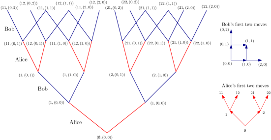
Consider a game played by two players, Alice and Bob, who take turns to play moves each. Alice starts. For each move, each player has two options. The outcome of the game is determined by the exact sequences of moves played by Alice and Bob. We assign a random winner to each of the possible outcomes of the game in an i.i.d. fashion. For each given outcome, the probability that Bob is the winner is . For later reference, we give this game the name . Since the game is finite, for each possible assignment of winners to outcomes, precisely one of the players has a winning strategy.444This is a basic result from game theory, that can easily be proved using the inductive formula (1.9) below. Let denote the probability that Bob has a winning strategy. Pearl [Pea80] showed that, setting , which has the effect that is the golden ratio,555In fact, setting , one has that and . one has that
| (1.1) |
Note that , which is due to the fact that Bob has the last move, which gives him an advantage.
Imagine now that we change the game in such a way that for the outcome of the game, the whole history of the moves played by Alice is relevant as before, but all that matters of Bob’s moves is the total number of times he plays each of the two possible moves. In this case, there are possible outcomes of the game. As before, we assign a winner independently to each possible outcome, where is the probability that Bob is the winner for a given outcome. We call this game and let denote the probability that Bob has a winning strategy. Similarly, we let denote the game in which the outcome is determined by how often Alice has played each of the two possible moves and by the whole history of the moves played by Bob. Finally, we let denote the game in which both for Alice and Bob, all that matters for the outcome is how often each of them has played each of the possible moves. We denote the probability that Bob has a winning strategy in these games by and , respectively.
It seems that if for the outcome of a game, all that matters is how often a player has played each of the two possible moves, then this player has less influence on the outcome compared to the game in which the whole history of moves played by this player matters. It is natural to conjecture that this gives such a player a disadvantage. Our first result partially confirms this.
Proposition 1 (Less influence on the outcome)
One has and for all and .
We conjecture that similarly and , but we have not been able to prove this.
From now on, we mostly focus on the games and . Our next result says that even though these games give Bob and Alice a disadvantage compared to the game , for values of close enough to one or zero, they still have with high probability a winning strategy. Moreover, similarly to (1.1), there is a sharp threshold of the parameter that separates two regimes where for large either Alice or Bob have with high probability a winning strategy.
Theorem 2 (Sharp threshold)
There exist constants such that
| (1.2) |
Contrary to (1.1), we have not been able to determine the limit behaviour as of at , but we know that the limit cannot be zero. Numerical data suggest the limit is either one or close to one, see Figure 1. For , the situation is similar except that the roles of 0 and 1 have been interchanged. Numerical simulations suggest that and . We have the following rigorous bounds.

Proposition 3 (Bounds on the thresholds)
One has and .
The bound comes from the following observation. We can partition the possible outcomes of the game into sets of elements each, such that Alice’s moves determine in which set the outcome lies, and then Bob’s moves determine the precise outcome within each set. The probability that all outcomes in a given set are a win for Alice is . Since there are sets, we see that if , then in the limit , with high probability, there is at least one set in which all elements are a win for Alice. This means that Alice has a particularly simple winning strategy: by choosing her moves in advance, she can make sure she wins without even having to react to Bob’s moves.
The proofs of the bounds and are a bit more complicated. We will use a Peierls argument first invented by Toom [Too80] and further developed in [SST22]. Toom’s Peierls argument was invented to study perturbations of monotone cellular automata started in the all-one initial state. In Toom’s original work, the time evolution is subject to random perturbations, but as was recently demonstrated by Hartarsky and Szabó in the context of bootstrap percolation [HS22], his method can also deal with perturbations of the initial state. To prove that the threshold in Theorem 2 is sharp, we will use an inequality from the theory of noise sensitivity first derived by Bourgain, Kahn, Kalai, Katznelson, and Linial [BK+92].
For the game our results are much less complete than for the games and . Using Toom’s Peierls argument, we are able to prove the following result, however.
Proposition 4 (Bounds for small and large parameters)
One has
| (1.3) |
The paper is organised as follows. In the remainder of the introduction, we discuss the graph structure of our games, we give an alternative interpretation of the quantities , , , and in terms of a cellular automaton, and we discuss related literature. Detailed proofs are deferred till Section 2.
1.2 The graph structure of the games
To describe the graph structure of our games of interest, we first introduce some general notation. Recall that a directed graph is a pair where is a set whose elements are called vertices and is a subset of whose elements are called directed edges. By a slight abuse of notation, we will sometimes use as a shorthand for , when it is clear how the set of directed edges is defined. We say that is finite if is a finite set. For we write if there exist such that for all . We let denote the smallest integer for which such exist. We say that is acyclic if there do not exist with such that . For , we adopt the notation and we write
| (1.4) |
Quite generally, we can describe the graph structure of a finite turn-based game played by two players by means of a quadruple where
-
(i)
is a finite acyclic directed graph,
-
(ii)
satisfies for all ,
-
(iii)
is a function.
For the sake of the exposition, let us call such a quadruple a game-graph. Slightly abusing the notation, we will sometimes write as shorthand for , when it is clear how is equipped with the structure of a game-graph. We call the root. We interpret as the set of possible states of the game, as the state at the beginning of the game, as the set of possible outcomes of the game, as the non-final states of the game, and as a function that tells us whose turn it is in each non-final state of the game. We write
| (1.5) |
A (pure) strategy for Alice is a function
| (1.6) |
which has the interpretation that in the state , Alice always plays the move that makes the game progress to the state . Likewise, a strategy for Bob is a function . We let (resp. ) denote the set of all strategies for Alice (resp. Bob). Given a strategy of Alice and a strategy of Bob, there is a unique sequence of vertices with and such that for each one has if and if . Then
| (1.7) |
is the outcome of the game if Alice plays strategy and Bob plays strategy . Given a function that assigns a winner to each possible outcome, with meaning that Alice is the winner and meaning that Bob is the winner, we say that a strategy is a winning strategy for Alice given if
| (1.8) |
Winning strategies for Bob are defined similarly (with instead of ). To find out who has a winning strategy given , we can work our way back from the set of all possible outcomes to the initial state of the game. Given a function that assigns a winner to each possible outcome, we can define by setting for and then defining inductively
| (1.9) |
Then it is not hard to see that Alice (resp. Bob) has a winning strategy if and only if (resp. ). We let denote the monotone Boolean function defined as
| (1.10) |
Then (resp. ) if Alice (resp. Bob) has a winning strategy given .
The game-graphs of the games that we are interested in have a special structure: the players alternate turns and play a fixed number of turns. Game graphs with various numbers of turns are consistent, in the sense that the game-graph of the game with turns can be obtained by truncating a certain infinite graph at height . Moreover, these infinite graphs have a sort of product structure, in the sense that they are the “product” of two directed graphs associated with the individual players. To describe this, it will be useful to introduce some more notation.
Let us define a decision graph to be a triple such that
-
(i)
is a directed graph,
-
(ii)
satisfies for all ,
-
(iii)
for all , with ,
-
(iv)
for all .
Note that (iii) implies that is acyclic. For a decision graph , we introduce the notation
| (1.11) |
Given a decision graph and integer , we can define a game-graph
| (1.12) |
by setting
| (1.13) |
which has the effect that and , and then defining
| (1.14) |
This corresponds to a game where Alice and Bob take turns to play moves together, and Alice starts. For the games we are interested in, has a product structure, in the sense that elements of are of the form where and record all that is relevant of Alice’s and Bob’s moves up to this point in the game. To formalise this, given two decision graphs ), we define a third decision graph by setting ,
| (1.15) |
and
| (1.16) |
The game-graphs of the games , , , and from the previous subsection are of the special form for a suitable choice of and . In fact, only two different choices for and occur, which we now describe.
Let denote the space of all finite words made up from the alphabet . We call the length of and we let denote the word of length . If and , then we let denote the concatenation of and . We view as a decision graph with vertex set , edge set
| (1.17) |
and root . Note that .
Let denote the set of all pairs of nonnegative integers. We view as a decision graph with vertex set , edge set
| (1.18) |
and root . Note that .
With this notation, the game-graphs of the games , , , and are given by
| (1.19) |
respectively. We let
| (1.20) |
denote the corresponding monotone Boolean functions, defined as in (1.10). Then
| (1.21) |
and the same holds with replaced by , , or . Here and similarly in the other three cases.
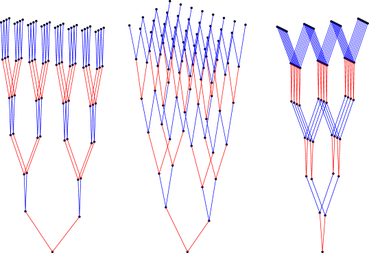
We observe that , i.e., the decision graph has the structure of a binary tree. This means that in the game , to each possible outcome leads a unique game history. On the other hand, in the games , , and , different game histories can lead to the same outcome. See Figures 2 and 3 for pictures of the game-graphs of the games and .
1.3 Cellular automata
In Subsection 1.1 we gave a somewhat informal description of the functions , , , and in terms of winning strategies. In formula (1.21) of Subsection 1.2 we gave an alternative description of these functions in terms of Boolean functions with i.i.d. input. In the present subsection we will give yet another representation of these functions in terms of cellular automata.
Let be the set of functions . Given a random variable with values in , we will be interested in a stochastic process that evolves in a deterministic way. At even times , we define in terms of according to one of the following two rules
| (1.22) |
and at odd times , we define according to one of the rules
| (1.23) |
The four possible combinations yield four possible ways to define a dynamic, which we denote by , , , and . Let be i.i.d. -valued random variables with , and let be defined according to the rules and with initial state . We claim that
| (1.24) |
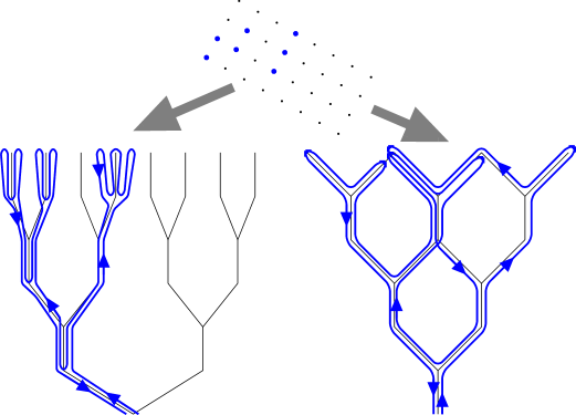
We only sketch the proof for the combination of rules . The main idea is to look at the “genealogy” of a space-time point . By rule , we have
| (1.25) |
where by rule ,
| (1.26) |
Continuing in this way, one can work out how is defined in terms of . A careful inspection of the rules (see Figure 4) shows that this leads precisely to the structure of the game-graph , so that (1.24) follows from (1.21). The proofs for the other combinations of rules are similar.

Because of the tree structure of the decision graph , it is easy to see that for the cellular automaton , one has that
| (1.27) |
Because of this, the analysis of the game is relatively simple. For the cellular automaton , we will prove in Lemma 16 below that it is still true that
| (1.28) |
but in the -direction dependencies develop. Because of this, the analysis of the game is more difficult and it seems unlikely that an explicit formula for the critial value can be found. The situation for the game is similar, while for the cellular automaton independence is lost in both directions.
There exists a nice way of coupling cellular automata with different initial intensities . Let be i.i.d. uniformly distributed -valued random variables. Then we can inductively define cellular automata with values in by applying at even times one of the rules
| (1.29) |
and at odd times one of the rules
| (1.30) |
Note that compared to (1.22) and (1.23), the minimum and maximum operations have been interchanged. Defining , , and so on in this way, it is straightforward to check that for each , setting
| (1.31) |
defines a cellular automaton with values in of the type described earlier. It follows therefore from (1.24) that
| (1.32) |
See Figure 5 for a numerical simulation of the cellular automaton .
This coupling has a nice interpretation in terms of a game. Let be a game-graph as defined in Subsection 1.2 and let be i.i.d. uniformly distributed -valued random variables, that have the interpretation that if the outcome of the game is , then Alice receives the pay-out and Bob receives the pay-out . If both players play optimally, then the game will end in some a.s. unique outcome , which is characterised by the fact that
| (1.33) |
where as in (1.7), denotes the outcome of the game if Alice plays strategy and Bob plays strategy . Specialising to the game-graphs from (1.19), we can in this way define random games , , , and where the pay-out of Alice and Bob for each outcome is determined by i.i.d. uniformly distributed -valued random variables. Then the random variable from (1.32) can be interpreted as Bob’s pay-out in the game if both players play optimally, and similarly for the games , , and .
1.4 Discussion and open problems
The game-graph of Pearl’s [Pea80] original game is the deterministic tree . Several authors have studied variants of the game where this tree is replaced by a random tree. Martin and Stasiński in [MS18] studied min-max games on a Galton-Watson tree, truncated at some height . Pemantle and Ward in [PW06] studied a model on a binary tree where i.i.d. random variables attached to the nodes determine whether the minimum or maximum function should be applied. We refer to Broutin and Mailler [BM18] for an overview of the literature on this type of problems.
For games with a large number of moves, it may be computationally unfeasible to find a winning strategy. This motivates the study of efficient algorithms that can play games near optimally. Indeed, this was the main motivation for Pearl [Pea80] to study the game . There is an extensive literature on this topic. We cite [DG95] for a somewhat older overview and [SN15, MS18] for more recent contributions.
When trying to play a game near optimally, a natural approach is to find all possible states that can be reached after a fixed number of moves, then attach a utility to each possible state using some statistical procedure, and finally use minimaxing in the spirit of (1.9) to compute utility values for all states that lie less than moves in the future. Surprisingly, it was discovered by Nau [Nau80] that when the game-graph is a tree, such algorithms can sometimes behave pathologically, in the sense that increasing leads to worse, rather than better game playing. This sort of pathology has been the subject of much further research [LBG12].
An early suggestion, that has not been pursued much, is that this sort of pathologies may be resolved if different game histories can lead to the same outcome [Nau83]. When the game no longer has the structure of a tree, however, independence is lost. For this reason, such games are harder to analyse and much less is known. There seems to be a general agreement, however, that introducing dependence may resolve game-playing pathology. For this reason, it would seem interesting to study game-playing algorithms for the games and introduced in the present paper.
Our own motivation for studying these games comes from a different direction, which is related to the cellular automata from Subsection 1.3. Attractive spin systems have two special invariant laws, called the lower and upper invariant laws, that are the long-time limit laws starting from the all zero and all one initial states [Lig85, Thm III.2.3]. If the dynamics of the spin system are invariant under automorphisms of the lattice (such as translations on ), then it is natural to ask if all invariant laws that are moreover invariant under automorphisms of the lattice are convex combinations of the lower and upper invariant laws. Frequently, one finds that mean-field models have an additional “intermediate” invariant law that lies between the lower and upper invariant laws, but very little is known about the existence of such intermediate invariant laws in a truly spatial setting. A notable exception are stochastic Ising models, where such intermediate invariant laws are known to exist if the lattice is a Cayley tree [Geo11, Section 12.2] but not on . (The latter follows from [Bod06] (in dimensions ) and [Hig81] (in dimension ) combined with [Lig85, Thm IV.5.12]; see also the discussion on [FV18, page 166]).
The cellular automaton from Subsection 1.3 is a mean-field model.666The cellular automaton , started from an i.i.d. law, remains i.i.d. for all time. This is characteristic of mean-field models (sometimes called “propagation of chaos”) and is closely related to the tree structure of the “genealogy” of . Compare the relation between recursive tree processes and mean-field limits in [MSS20]. It has an intermediate invariant law, which is the product measure with intensity . Our original plan was to prove that the cellular automata and also have an intermediate invariant law, but this is still unresolved. This is closely related to the question about the limit behaviour of at . We have shown that this quantity does not tend to zero. It seems there are two plausible scenarios: either this quantity tends to one and the cellular automaton has no intermediate invariant law, or it tends to a value strictly between zero and one and such an intermediate invariant law exists.
Another open problem concerns the size of the “critical window” where the function changes from a value close to zero to a value close to one. In Theorem 14 below, we prove an upper bound of order , but it is doubtful this is sharp, given that for the game the size of the critical window decreases exponentially in . For the mean-field game , a detailed analysis of the critical behaviour, which involves a nontrivial limit law, has been carried out in [ADN05].
There are lots of open problems concerning the game . Below Proposition 1 we already mentioned the conjecture that and for all and . Another obvious conjecture is the existence of a critical value such that
| (1.34) |
Our proof of Theorem 2 uses the special structure of the game-graphs associated with the games and in two places: namely, in the preparatory Lemmas 15 and 18 we use that the game-graphs have a product structure with one component a binary tree. Based on numerical simulations, we conjecture that a critical value as in (1.34) exists and that the cellular automaton started in product law with this intensity converges as time tends to infinity to a convex combination of the delta-measures on the all-zero and all-one states. Based on this, we conjecture that the cellular automaton has no intermediate invariant law.
2 Proofs
2.1 An inequality for monotone Boolean functions
In this subsection we prepare for the proof of Proposition 1 by establishing a general comparison result for monotone Boolean functions applied to i.i.d. input.
A Boolean variable is a variable that takes values in the set . A Boolean function is any function that maps a set of the form , where is a finite set, into . A Boolean function is monotone if (pointwise) implies . Let be a monotone Boolean function. By definition, a one-set of is a set such that , where denotes the indicator function of , and a zero-set of is a set such that . A one-set (respectively zero-set) is minimal if it does not contain other one-sets (respectively zero-sets) as a proper subset. We let and denote the set of one-sets and zero-sets of , respectively, and we denote the sets of minimal one-sets and zero-sets by and , respectively.777This notation is motivated by the fact that by the monotonicity of and also by the desire to have a simple notation for which is needed more often than . We will prove the following result.
Proposition 5 (An inequality)
Let and be finite sets and let be a monotone Boolean function. Let be a function such that
| (2.1) |
and let and by i.i.d. collections of Boolean random variables with intensity . Then
| (2.2) |
Similarly, if (2.1) holds with minimal one-sets replaced by minimal zero-sets, then (2.2) holds with the reversed inequality.
The proof of Proposition 5 needs some preparations. If are distinct elements of and , then we let denote the function
| (2.3) |
We let and denote the functions from to defined as
| (2.4) |
For each , we let denote the inverse image of under .
Lemma 6 (Contraction of two points)
In addition to the assumptions of Proposition 5, assume that there exist two elements and an element such that and for all . Then
| (2.5) |
Proof Let , and denote the functions from to defined as
| (2.6) |
. Then it is easy to check that are all monotone Boolean functions from . Using the fact that the collection is i.i.d. with intensity , we see that
| (2.7) |
Similarly
| (2.8) |
Subtracting yields (2.5).
Proof of Proposition 5 It suffices to prove the statement for minimal one-sets. The statement for minimal zero-sets then follows by the symmetry between zeros and ones. Let us say that is a pair contraction if is surjective and . We first prove the statement under the additional assumption that is a pair contraction.
If is a pair contraction, then there exist two elements and an element such that and for all , so Lemma 6 is applicable and (2.2) follows from (2.5) provided we show that for all . Assume that for some . Since only depends on the values of for , we can without loss of generality assume that . Define by
| (2.9) |
Then implies that while . This is possible only if for some , which contradicts (2.1). This completes the proof in the special case that is a pair contraction.
Before we prove the general statement, we make some elementary observations. If are finite sets and is a function, then we can define by . With this notation, (2.2) takes the form
| (2.10) |
We claim that
| (2.11) |
Indeed, for each , one has
| (2.12) |
and the implication here can only hold for all if (2.11) is satisfied.
We now prove that (2.1) implies (2.10). We can without loss of generality assume that is surjective. Then we can find an integer , finite sets with and , and pair contractions , such that . For each , let and be defined as
| (2.13) |
where is the identity map. For each , let be an i.i.d. collection of Boolean random variables with intensity . We will prove (2.10) by showing that
| (2.14) |
Since with , it suffices to show that
| (2.15) |
Since is a pair contraction, by what we have already proved, it suffices to show that
| (2.16) |
The assumption (2.1) implies that and hence for all . In view of (2.11), for each , there exists an such that . The fact that now implies (2.16) and the proof is complete.
2.2 Comparison with the game on a tree
In this subsection we prove Proposition 1. We will apply Proposition 5 to the monotone Boolean function from (1.20). We start with some general observations.
Let be a game-graph and let be the monotone Boolean map defined in (1.10). Using notation from Subsection 1.2, let and denote the set of strategies of Alice and Bob, respectively, and as in (1.7) let denote the outcome of the game if Alice plays strategy and Bob plays strategy . For each and , we let
| (2.17) |
denote the sets of possible outcomes of the game if Alice plays the strategy or Bob plays the strategy , respectively. We make the following simple observation.
Lemma 7 (Strategies and zero-sets)
Let
| (2.18) |
Then
| (2.19) |
Proof By symmetry, it suffices to prove the statement for zero-sets. We claim that
| (2.20) |
Indeed, using the fact that if and only if Alice has a winning strategy given , we see that
which proves (2.20). As an immediate consequence, we obtain
i.e., .
To prove that , assume that . Then, since (2.20) implies that there exists a such that . Since we have , so the minimality of implies , proving that .
Lemma 8 (Projection property)
Let and be decision graphs and assume that satisfies
| (2.21) |
Let and let and be the Boolean functions defined as in (1.10) in terms of the game-graphs and , respectively. Then for each , maps into , and
| (2.22) |
where is defined as .
Proof It is easy to see that (2.21) implies that . As a result, maps into . We can inductively extend the function to a function such that for all ,
| (2.23) |
Then . Define by . Then as a result of (2.21), we see that satisfies the inductive relation
| (2.24) |
Letting denote the restriction of to , it follows that
| (2.25) |
An example of a function satisfying (2.21) is the function defined as
| (2.26) |
Further examples are the functions and defined as
| (2.27) |
where is as in (2.26). Lemma 8 now tells us that
| (2.28) |
We wish to apply Proposition 5 to and or . The following special property of the game-graph will be crucial in our proof of Proposition 1.
Lemma 9 (The game-graph that is a tree)
For the game-graph , let and be strategies for Alice and Bob, respectively, and let and be defined as in (2.17). Then for each , there exists precisely one such that . Likewise, for each , there exists precisely one such that .
Proof To prove the first statement, let be a strategy for Alice and let . Because of the tree structure of , given , we know exactly which moves Bob must make in each of his turns for the outcome of the game to be of the form for some . Since we also know Alice’s strategy, this means that we have all necessary information to determine the outcome of the game. This shows that is unique. On the other hand, it is easy to see that there exists at least one strategy for Bob that leads to the outcome . This completes the proof of the first statement. The second statement follows from the same argument.
Proof of Proposition 1 Let
| (2.29) |
be i.i.d. collections of Boolean random variables with intensity . We claim that
| (2.30) |
Indeed, the first and final equalities follow from formula (1.21), the second equality follows from formula (2.28), and the inequality will follow from Proposition 5 provided we show that
| (2.31) |
We claim that (2.31) follows from Lemmas 7 and 9. Indeed, Lemma 9 implies that each has the property that for each , there exists precisely one such that , so by Lemma 7 the same is true for each . Since acts only on the second coordinate, this implies (2.31). This completes the proof that . The proof that follows from the same argument.
2.3 Toom cycles
In Subsection 2.5, we will derive upper bounds on the probability that Alice has a winning strategy in the games and , and on the probability that Bob has a winning strategy in the games and , which then translate into some of the bounds in Propositions 3 and 4. To have a unified set-up, it will be convenient to introduce games and that are identical to the games and except that instead of Alice, Bob starts. Then the probability that Bob has a winning strategy in the games and is equal to the probability that Alice has a winning strategy in the games and , respectively. Therefore, it suffices to derive upper bounds on the probability that Alice has a winning strategy in the games , , , and .
We will use a Peierls argument first invented by Toom [Too80] and further developed in [SST22]. To prepare for this, in the present subsection, we formulate a theorem that says that if Alice has a winning strategy in any of these games, then a certain structure must be present in the game-graph that following [SST22] we will call a “Toom cycle”. We first need to introduce notation for the game-graphs of the games and .
Given a decision graph and integer , we define a game-graph
| (2.32) |
exactly as in (1.13), but with (1.14) replaced by
| (2.33) |
In (1.15) and (1.16), we defined a sort of “product” of two decision graphs and . Elements of are pairs with and . If is at distance from the root, then to reach a new state at distance from the root, we replace either or by a new state or in or that lies one step further from the root. Here we replace in case is even and in case is odd, as is natural for a game where Alice starts. For games where Bob starts, very much in the same spirit, we can define a second “product” which differs from only in the fact that we replace in case is odd and in case is even. Formally, we set
| (2.34) |
which is then equipped with the structure of a decision graph in the obvious way. We will be interested in the game-graphs
| (2.35) |
Note that in each case, the decision graph of Bob is . We do not insist that is even, so we also allow for games where the same player has both the first and the last move. We will show that given a function that assigns winners to possible outcomes, if Alice has a winning strategy, then a “Toom cycle” must be present in these game-graphs.
Fix and let be any of the game-graphs in (2.35). Elements of are pairs with an element of or and an element of . Recall that if and , then denotes the word obtained by appending the letter to the word . To have a unified notation, it will be convenient to introduce for the decision-graph the notation
| (2.36) |
Recall that and are the sets of internal states when it is Alice’s and Bob’s turn, respectively. Using notation as in (2.36), we set for
| (2.37) |
and write and so that . For any set of directed edges , we let
| (2.38) |
denote the set of directed edges obtained by reversing the direction of all edges in . A walk in of length is a finite word made from the alphabet such that for each . We call the substring the -th step of the walk and we say that the -th step is:
-
straight-up (su) if , straight-down (sd) if ,
-
left-up (lu) if , left-down (ld) if ,
-
right-up (ru) if , right-down (rd) if .
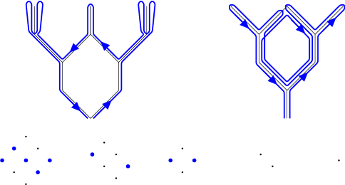
This terminology is inspired by the right picture in Figure 6. Steps of the types su, ru, and lu are called up and steps of the types sd, ld, and rd are called down. Steps of the types su and sd are called straight, those of the types lu and ld left, and those of the types ru and rd right. For any walk , we set and we partition into subsets defined as
| (2.39) |
We next define Toom cycles. A Toom cycle in is a walk in of length that must satisfy a number of requirements. First, we require that
| (2.40) |
Next for , depending on the type of the -th step and on whether or , we will put constraints on the type of the -th step. More precisely, if , then only the following combinations are allowed for the types of the -th and the -th step:
| (2.41) |
If, on the other hand, , then only the following combinations are allowed:
| (2.42) |
See Figure 6 for an illustration. Note that these rules imply that . In addition to the requirements above, a Toom cycle has to fulfill the following two additional, final requirements:
-
(i)
for all with ,
-
(ii)
if for some and with and with respect to the total order on defined by , then .
Requirement (i) says that vertices in are visited only once. Applying (ii) twice we see that if for some with , then , so (ii) can roughly be described by saying that internal vertices can be visited at most three times, and these visits have to take place in the right order depending on whether the walk is going up, is in a local minimum, or goes down.
Given a function that assigns a winner to each possible outcome, we say that a Toom cycle is present in if
| (2.43) |
We will prove the following theorem.
Theorem 10 (Toom cycles)
Let be any of the game-graphs in (2.35) and let be a function that assigns a winner to each possible outcome. If Alice has a winning strategy given , then a Toom cycle is present in .
One can check that in Theorem 10, the converse implication does not hold, i.e., the presence of a Toom cycle does not imply that Alice has a winning strategy. A counterexample for the game-graph is shown in Figure 7. Intriguingly, we have not been able to construct a counterexample for the game-graphs and , leaving open the possibility that the converse implication holds in these cases. Theorem 10 is very similar to [SST22, Thm 9] and so is its proof (see in particular [SST22, Figure 4] for the idea of loop erasion), but since our setting is different and we will need some special properties of Toom cycles that are specific to our setting we will give an independent proof here. Strategies for Alice have an analogue for general monotone cellular automata. In this general context, they correspond to the so-called “minimal explanations” of [SST22, Section 7.1], whose relation to Toom cycles is discussed in more detail in that article. We prove Theorem 10 in Subsection 2.4 and then apply it in Subsection 2.5.
2.4 Presence of Toom cycles
In this subsection we prove Theorem 10. Let be any of the game-graphs in (2.35) and let be defined as in (1.10), i.e., this is the Boolean function defined by the requirement that if be a function that assigns a winner to each possible outcome, then if and only if Alice has a winning strategy given . Using notation introduced in Subsection 2.1, let denote the set of zero-sets of and let denote its set of minimal zero-sets. Defining as in (2.18), we recall from Lemma 7 that
| (2.44) |
Remark One can check that both inclusions in (2.44) are strict. We say that a strategy for Alice is minimal if the set from (2.17) satisfies . Note that regardless of how one assigns winners to possible outcomes, it actually never makes sense for Alice to play a strategy that is not minimal, since for each non-minimal strategy she has at her disposal another strategy that is guaranteed to be at least as good in each situation. For the game-graphs and , it seems that with some effort, it is possible to give a precise description of all minimal strategies for Alice, but for the game-graphs and , classifying the minimal strategies seems a hard task.
Proof of Theorem 10 For each Toom cycle , we write
| (2.45) |
and we set
| (2.46) |
We will prove that
| (2.47) |
which clearly implies the statement of the theorem. The proof is by induction on . For concreteness, we write down the proof for the game-graphs and , and at the end remark on how the proof has to be adapted for the other two game-graphs. To have a unified notation, we write where or . Let and denote the sets defined in (2.18) and (2.46) for a given value of . It will be convenient to also include the case . For this purpose, we use the convention that in this case there is precise one Toom cycle, which is the walk of length given by , where denotes the root of . Then and both have a single element, which is the singleton , and (2.47) holds for .
If is even, is given, and is a function, then we can define by
| (2.48) |
where is defined as in (2.36) if the decision graph of Alice is . Formula (2.48) corresponds to Alice playing the strategy that defined up to the -th turn of the game and then playing the move if at that moment the state of the game is . We see from this that , and each element of is of this form for some . Similarly, if is odd and is given, then we can define by
| (2.49) |
Indeed, this corresponds to Alice playing the strategy that defined up to the -th turn of the game, while Bob has now one extra final move. We see from this that , and each element of is of this form for some . In view of this, to complete the induction step of the proof, it suffices to show that:
To prove this, let be a Toom cycle such that . If is even, then we modify in such a way that for each such that , in place of we insert the string . Note that this adds two steps to the Toom cycle, the first of which is straight-up and the second straight-down. If is odd, then we modify in such a way that for each such that , in place of we insert the string . Note that this adds four steps to the Toom cycle: right-up, left-down, left-up, and right-down.
Let denote the modified walk. Then it is straightforward to check that and satisfies all requirements of a Toom cycle, except possibly for requirement (i), i.e., it may now be the case that some potential outcomes of the game are visited more than once. To remedy this, we apply the procedure of loop erasion which is also the main idea behind the proof of [SST22, Thm 9]. If for some , then we remove the string from . One can check that this preserves all the requirements of a Toom cycle that satisfies. Moreover, by applying this procedure till it is no longer possible to do so, we can make sure that also requirement (i) becomes valid again. In this way, we find a new modified Toom cycle such that . Note, however, that because of the loop erasion, even if we started with , it may happen that is a strict subset of .
The proof for the game-graphs and is essentially the same. It differs only in the sense that the roles of even and odd are interchanged.
Remark For the game-graphs and , one can check that because of the loop erasion, the construction in the proof of Theorem 10 can yield Toom cycles in which a right-up step is followed by a right-down step, as explicitly allowed in (2.42). For the game-graphs and , it seems that on the other hand such transitions never arise from the construction in the proof of Theorem 10, so for these game-graphs it should be possible to prove a stronger version of the theorem in which the Toom cycle satisfies additional properties. Since we do not need this for our main results, we do not pursue this further.
2.5 The Peierls argument
Recall the definition of the games and at the beginning of Subsection 2.3. In this subsection, we apply Theorem 10 to derive upper bounds on the probability that Alice has a winning strategy in the games , , , and . We start by considering game-graphs where Alice starts, since in this case the argument is slightly easier.
Lemma 11 (Toom cycles if Alice starts)
If is a Toom cycle in or , then there exists an integer such that the number of steps of each of the types su, sd, lu, ld, ru, rd equals , and the Toom cycle passes through precisely different possible outcomes of the game.
Proof We see from (2.41) and (2.42) that after a step of a type in there always follows a step of a type in and vice versa. Therefore, since the first step of the Toom cycle is straight-up and the last step is straight-down, the number of steps of the Toom cycle is even and if we divide its steps in pairs of two consecutive steps, then the first step of such a pair is always of a type in and the second step of a type in . It follows from the structure of and that a straight-up step cannot end in , so by (2.41) only three types of pairs of two consecutive steps are possible:
| (2.50) |
By a slight abuse of notation, let us also write to denote the number of straight-up steps in the Toom cycle, and similarly for the other five types of steps. Then (2.50) implies that
| (2.51) |
Since the distance from the root increases by one in each up move and decreases by one in each down move, and the cycle ends where it began, the number of up moves must equal the number of down moves, which gives
| (2.52) |
Similarly, if denotes the difference between number of 1 moves and 2 moves played by Bob when the state of the game is , then the function increases by one in each right move, decreases by one in each left move, and stays the same in straight moves, so we see that the number of right moves must equal the number of left moves, which gives
| (2.53) |
Combining (2.51), (2.52), and (2.53), we see that there exists an integer such that
| (2.54) |
In view of (2.41), each change from the down direction to the up direction is associated with a pair consisting of a left-down step followed by a left-up step, so the number of these changes is precisely . Since the first step is up and the last step is down, we change from the up direction to the down direction once more than the other way around. Because of (2.41) and (2.42), changes from the up direction to the down direction can only happen in states that are a possible outcome of the game, and because of the crucial condition (i) in the definition of a Toom cycle, the walk visits each possible outcome at most once. It follows that the Toom cycle passes through precisely different possible outcomes of the game.
Proposition 12 (Peierls estimates if Alice starts)
For each , the probability that Alice has a winning strategy in the games and can be estimated from above by
| (2.55) |
In particular,
| (2.56) |
Proof Let and let be i.i.d. Boolean random variables with intensity . By Theorem 10, the probability that Alice has a winning strategy in the game can be estimated from above by the probability that a Toom cycle is present in , which in turn can be estimated from above by the expected number of such Toom cycles. By Lemma 11, the length of such a Toom cycle must be of the form with an integer. We have since the cycle must make at least straight-up steps before it can start walking down. Since by Lemma 11, a Toom cycle of length visits precisely possible outcomes, the probability that a given Toom cycle of length is present in is precisely . This gives the bound
| (2.57) |
where denotes the number of distinct Toom cycles of length in . We claim that
| (2.58) |
Here the first factor comes from the fact that for each straight-up step we have two choices (corresponding to the two possible moves of Alice), the second factor comes from the fact that each time we arrive in a possible outcome of the game, we have to choose whether the next step is left-down or right-down, and the third factor comes from the fact that after each straight-down step except the very last one, we have to choose whether the next step is left-down or right-down. By (2.41) and (2.42) these are the only choices we need to make to uniquely determine a Toom cycle.
The argument for the game is precisely the same, except that now the decision graph of Alice is no longer a tree which has the effect that also at the beginning of each straight-down step we may have to choose between two possible ways of making a straight-down step (see Figure 7).
For the game-graphs where Bob starts, the argument is only slightly more complicated.
Proposition 13 (Peierls estimates if Bob starts)
For each , the probability that Alice has a winning strategy in the games and can be estimated from above by
| (2.59) |
As a result,
| (2.60) |
Proof The proof is very similar to the proof of Proposition 12, but we have to modify Lemma 11. Toom cycles in the game-graphs and can be obtained from Toom cycles in the game-graphs and by removing the first and last steps (which were straight-up and straight-down), and then inserting at each instance where the Toom cycle changes from the up to the down direction one extra straight-up step followed my a straight-down step. The argument then proceeds as before up to the point where we count the number of modified Toom cycles for which the original (unmodified) Toom cycle had length . For the game-graph , we get a factor for each straight-up step. Due to the modification, the number of straight-up steps has decreased by one and increased by , so we gain an extra factor . For the game-graph , we also get a factor for each straight-down step, so we gain a factor . This explains (2.59).
2.6 Sharpness of the transition
Throughout this subsection, denotes any of the game-graphs and , which are the game-graphs of the games and , respectively, and denotes any of the Boolean functions and that tell us who has a winning strategy for each given assignment of winners to possible outcomes, with and indicating a win for Alice and Bob, respectively.
For each , we let be i.i.d. Boolean variables with intensity and for each , we define
| (2.61) |
. By definition, a possible outcome is pivotal for if , which by the monotonicity of means that and . The influence of is defined as
| (2.62) |
and Russo’s formula (see, e.g., [GS14, Thm 3.2]) tells us that the probability that Bob has a winning strategy is continuously differentiable with
| (2.63) |
It is easy to see that each possible outcome has a positive influence, so Russo’s formula implies that is strictly increasing. Since moreover and , we conclude that the function is invertible. We will prove the following result.
Theorem 14 (Sharpness of the transition)
For each , there exists a constant such that
| (2.64) |
We start with a preparatory lemma.
Lemma 15 (Lower bound on the total influence)
There exists a constant such that for all , one has
| (2.65) |
Proof Let us write
| (2.66) |
For the game-graph , the set of possible outcomes is , where has elements that play a completely symmetric role in , so that the influence of an element depends on but not . Choosing such that for all gives the trivial bound
| (2.67) |
For the game-graph , we get the same bound by reversing the roles of and . To complete the proof, we apply an inequality from the theory of noise sensitivity. By [GS14, Thm 3.4], which is based on [BK+92], there exists a universal constant such that
| (2.68) |
Combining these two estimates one arrives at (2.65).
Proof of Theorem 14 Since is strictly increasing we have
| (2.69) |
Russo’s formula (2.63) and Lemma 15 now tell us that there exists a constant such that
| (2.70) |
Making smaller if necessary, we can without loss of generality assume that
| (2.71) |
To estimate the right-hand side of (2.70) from below, we set . Since the function is increasing and is decreasing, we have
| (2.72) |
We observe that by (2.71),
| (2.73) |
Choose . Then (2.70), (2.72), and (2.71) combine to give
| (2.74) |
Setting , we obtain (2.64).
2.7 The cellular automata
In this subsection we study the cellular automata and from Subsection 1.3. It will be convenient to change the notation a bit. Given a random variable with values in , we can define a discrete-time process with values in by setting
| (2.75) |
In particular, if are i.i.d. with intensity , then this is the cellular automaton defined in Subsection 1.3. Similarly, given a random variable with values in , we can define a discrete-time process with values in by setting
| (2.76) |
where compared to (2.75) all we have done is that we have interchanged the rules at even and odd times. The cellular automaton is similar to the cellular automaton from Subsection 1.3, but compared to the definitions there, the roles of and and the roles of and are interchanged. More precisely, if are i.i.d. with intensity , then setting
| (2.77) |
yields a cellular automaton as defined in Subsection 1.3.
As observed in (1.28), the cellular automaton has the property that at each time its columns are independent. This holds not only for product initial laws but more generally if the initial state has the property that its columns are independent, and the same holds for . This motivates the following definitions.
We let denote the space of all functions . We equip with the product topology and the associated Borel--field and we set
| (2.78) |
We equip with the topology of weak convergence of probability laws. Then is a closed subset of . We define maps and by
| (2.79) |
we define maps and from to by
| (2.80) |
and we set
| (2.81) |
The following lemma is a more precise formulation of the observation (1.28).
Lemma 16 (Law of the columns)
Proof The proof is by induction on . Assuming that the statement holds for , we see from (2.75) that
| (2.84) |
which implies (compare Figure 4) that
| (2.85) |
Using again (2.75), we see that
| (2.86) |
which implies (2.83). The proof for is the same, but we apply and in the opposite order.
We let denote the product measure on with intensity and for any , we let which by stationarity does not depend on . Then our main functions of interest can be expressed in terms of the “column maps” and as
| (2.87) |
where the first equality follows from (1.24), Lemma 16, and the fact that started in product measure with intensity is the cellular automaton from Subsection 1.3, and in the second equality we have used (2.77).
Recall that is equipped with the product topology, is equipped with the topology of weak convergence, and denotes the set of stationary measures.
Lemma 17 (Properties of the column maps)
The maps , , , and are continuous with respect to the topology on and map into itself.
Proof In view of (2.81) it suffices to prove the statement for and . Preservation of stationarity is obvious. To prove continuity, assume that . By Skorohod’s representation theorem [Bil99, Thm 6.7], we can find random variables with laws such that a.s. with respect to the topology on . Let be an independent copy of and let be the a.s. limit of . Then a.s. and a.s. with respect to the topology on , which implies that and .
Lemma 18 (Upper bound on the density)
One has
| (2.88) |
and consequently,
| (2.89) |
Proof Let and be independent random variables with law . Then
| (2.90) |
and
| (2.91) |
, proving (2.88). It follows that
| (2.92) |
Let denote the configurations that are constantly zero and one, respectively. Since and , the delta-measure on is a fixed point of the maps and and hence also of and . The same applies to the delta-measure on . We define the domains of attraction of these fixed points as
| (2.93) |
where denotes weak convergence of probability measures on . The following proposition is the main result of this subsection.
Proposition 19 (Domains of attraction)
and are open, dense subsets of .
Proof Let . Since is a bounded continuous function, the map is continuous with respect to weak convergence of probability measures, and hence , being the inverse image of under this map, is an open subset of . We claim that
| (2.94) |
Indeed, the inclusion follows from the fact that is an open set containing and the inclusion follows from the fact that by Lemma 18. Since the map is continuous by Lemma 17, the inverse image of under the map is open for each , and hence
| (2.95) |
being a union of open sets, is open. The same argument shows that also is an open subset of .
We observe that the map is linear but is not. It is easy to check that for any , we have
| (2.96) |
Using the linearity of , we see that the same formula holds with replaced by or . It follows that
| (2.97) |
which shows that for all . Since as , and is arbitrary, we conclude that is dense in . The proof for is the same.
2.8 Proof of the main results
In this subsection we prove the results stated in Subsection 1.1 that have not been proved yet. Proposition 1 has already been proved in Subsection 2.2 and Proposition 4 follows from Propositions 12 and 13, so it remains to prove Theorem 2 and Proposition 3.
Proof of Theorem 2 and Proposition 3 We first prove the results for the game . Since the map from (1.20) is monotone with and , formula (1.21) tells us that the set
| (2.98) |
is an interval containing but not . By formula (2.87),
| (2.99) |
so Proposition 19 tells us that is an open set. It follows that there exists a constant such that
| (2.100) |
We recall from the discussion above Theorem 14 that is strictly increasing and so also invertible. We observe that if , then by formula (2.87) and Lemma 18,
| (2.101) |
which proves that
| (2.102) |
It follows that the increasing limit
| (2.103) |
exists in , and using Theorem 14 we see that
| (2.104) |
which implies that
| (2.105) |
Combining this with (2.100) we see that . Proposition 12 implies that , while the bound follows from the simple argument given in the text below Proposition 3. This completes the proofs for the game .
For the game , the arguments are similar. In this case, by formula (2.87),
| (2.106) |
is an open interval containing but not . Combining this with Lemma 18 and Theorem 14, the arguments above show that there exists a such that
| (2.107) |
Proposition 13 implies that and the bound follows from (1.1) and Proposition 1.
Acknowledgments
N. Cardona-Tobón would like to express her gratitude to the University of Göttingen, where she was a postdoctoral researcher during the preparation of this paper. Additionally, she would like to thank the Institute of Information Theory and Automation for its hospitality during her research stay in 2023, which was supported by the Dorothea Schlözer program of the University of Göttingen. J.M. Swart is supported by grant 22-12790S of the Czech Science Foundation (GA CR). We thank Gerold Alsmeyer for bringing the reference [ADN05] to our attention.
References
- [ADN05] T. Ali Kahn, L. Devroye, and R. Neininger. A limit law for the root value of minimax trees. Electron. Comm. Probab. 10 (2005), 273–281.
- [Bil99] P. Billingsley. Convergence of Probability Measures. 2nd edition, John Wiley & Sons Inc., New York, 1999.
- [BK+92] J. Bourgain, J. Kahn, G. Kalai, Y. Katznelson, and N. Linial. The influence of variables in product spaces. Israel J. Math. 77 (1992), 55–64.
- [BM18] N. Broutin and C. Mailler. And/or trees: A local limit point of view. Random Structures & Algorithms. 53 (2018) 15–58.
- [Bod06] T. Bodineau. Translation invariant Gibbs states for the Ising model. Probab. Theory Relat. Fields 135(2) (2006), 153–168.
- [DG95] C.G. Diderich and M. Gengler. A Survey on Minimax Trees And Associated Algorithms. Pages 25–54 in: D.Z. Du and P.M. Pardalos (eds) Minimax and Applications. Nonconvex Optimization and Its Applications 4. Springer, Boston, 1995.
- [FV18] S. Friedli and Y.Velenik. Statistical mechanics of lattice systems. A concrete mathematical introduction. Cambridge University Press, 2018.
- [Geo11] H.-O. Georgii. Gibbs measures and phase transitions. 2nd extended ed. De Gruyter, Berlin, 2011.
- [GS14] C. Garban and J.E. Steif. Noise Sensitivity of Boolean Functions and Percolation. Cambridge University Press, 2014.
- [Hig81] Y. Higuchi. On the absence of non-translation invariant Gibbs states for the two-dimensional Ising model. Pages 517–534 in: Random fields. Rigorous results in statistical mechanics and quantum field theory, Esztergom 1979. Colloq. Math. Soc. Janos Bolyai 27 (1981).
- [HS22] I. Hartarsky and R. Szabó. Subcritical bootstrap percolation via Toom contours. Electron. Commun. Probab. 27 (2022), 1–13.
- [LBG12] M. Luštrek, I. Bratko, and M. Gams. Independent-valued minimax: Pathological or beneficial? Theor. Comput. Sci. 422 (2012), 59–77.
- [Lig85] T.M. Liggett. Interacting Particle Systems. Springer-Verlag, New York, 1985.
- [MS18] J.B. Martin and R. Stasiński. Minimax functions on Galton-Watson trees. Combinatorics, Probability and Computing 29 (2020), 455–484.
- [MSS20] T. Mach, A. Sturm, and J.M. Swart. Recursive tree processes and the mean-field limit of stochastic flows. Electron. J. Probab. 25 (2020) paper No. 61, 1–63.
- [Nau80] D.S. Nau. Pathology on Game Trees: A Summary of Results. Pages 102–104 in: Proc. First Annual National Conference on Artificial Intelligence, Stanford, California, 1980.
- [Nau83] D.S. Nau. On game graph structure and its influence on pathology. Int. J. Comput. Inform. Sci. 12 (1983), 367–383.
- [Pea80] J. Pearl. Asymptotic properties of minimax trees and game-searching procedures. Artificial Intelligence 14(2) (1980), 113–138.
- [PW06] R. Pemantle and M.D. Ward. Exploring the average values of Boolean functions via asymptotics and experimentation. 2006 Proceedings of the Third Workshop on Analytic Algorithmics and Combinatorics (ANALCO). (2006) 253–262.
- [SN15] T. Suzuki and Y. Niida. Equilibrium points of an AND–OR tree: Under constraints on probability. Ann. Pure Appl. Logic 166(11) (2015), 1150–1164.
- [SST22] J.M. Swart, R. Szabó, and C. Toninelli. Peierls bounds from Toom contours. Preprint (2022) arXiv:2202.10999.
- [Too80] A.L. Toom. Stable and attractive trajectories in multicomponent systems. Pages 549–575 in: R.L. Dobrushin and Ya.G. Sinai (eds). Multicomponent random systems. Adv. Probab. Relat. Top. 6. Dekker, New York, 1980.