Rate-Adaptive Generative Semantic Communication Using Conditional Diffusion Models
Abstract
Recent advances in deep learning-based joint source-channel coding (DJSCC) have shown promise for end-to-end semantic image transmission. However, most existing schemes primarily focus on optimizing pixel-wise metrics, which often fail to align with human perception, leading to lower perceptual quality. In this letter, we propose a novel generative DJSCC approach using conditional diffusion models to enhance the perceptual quality of transmitted images. Specifically, by utilizing entropy models, we effectively manage transmission bandwidth based on the estimated entropy of transmitted symbols. These symbols are then used at the receiver as conditional information to guide a conditional diffusion decoder in image reconstruction. Our model is built upon the emerging advanced mamba-like linear attention (MLLA) skeleton, which excels in image processing tasks while also offering fast inference speed. Besides, we introduce a multi-stage training strategy to ensure the stability and improve the overall performance of the model. Simulation results demonstrate that our proposed method significantly outperforms existing approaches in terms of perceptual quality.
Index Terms:
Semantic communications, conditional diffusion models, joint source-channel coding, image transmission.I Introduction
The rapid development of sixth-generation (6G) communication systems has driven the rise of various smart applications, such as Virtual Reality (VR) and the Internet of Everything (IoE) [1, 2, 3, 4]. These services demand enhanced communication efficiency to manage the massive inflow of data traffic. In this context, semantic communications have emerged as a new paradigm, attracting significant attention. Unlike traditional transmission systems that rely on separate source and channel coding, semantic communications focus on accurately transmitting the underlying semantic information of digital data. This approach integrates source and channel coding for joint optimization, a technique known as joint source-channel coding (JSCC).
Recently, the integration of deep learning into wireless communication system designs has gained traction, driven by the exceptional information processing capabilities of various deep learning models. In this context, deep learning-based JSCC (DJSCC) has stimulated significant interest, particularly through the use of autoencoders (AEs) and their variants, such as variational AEs (VAEs). DJSCC maps input images into low-dimensional symbol vectors for transmission. A pioneering work in this area is DeepJSCC[2], which is built on an AE-based framework that allows for joint optimization and mitigates the cliff-edge effect commonly observed in traditional separation-based schemes. Moreover, the authors in [4] introduced a Transformer-based framework that enhances image fidelity by incorporating channel feedback to adaptively reconstruct images under varying wireless conditions. Inspired by entropy model-based source coding [5], the authors in [6] proposed a rate-adaptive JSCC system, where the number of transmitted symbols is determined by the entropy estimated by the entropy models. This work was further evolved in [7] into a digital version, enabling practical application in modern digital systems.
Despite the superior performance of current DJSCC transmission systems, they are typically optimized for mean-square error (MSE) distortion metrics such as peak signal-to-noise ratio (PSNR), which assesses pixel-level similarity between reconstructed and source images. However, it is increasingly recognized that high pixel-level similarity does not necessarily indicate high perceptual quality, which reflects how humans perceive the image’s realism and visual appeal [8]. To improve the perceptual quality of transmitted images, the authors in [9] introduced adversarial and perceptual losses into DJSCC. Moreover, [10] developed a dual-path framework to extract both pixel-level information and perceptual information. Alternatively, [11] combined DJSCC with the denoising diffusion probabilistic model (DDPM) [12], a powerful generative model that creates images from Gaussian noise. In [11], the reconstructed image is split into two components: range-space and null-space. The range-space that captures the primary structure is transmitted via DJSCC, while the null-space, refining details, is generated at the receiver using diffusion models. Another approach, presented in [13], leveraged diffusion models by first performing an initial reconstruction with DJSCC, followed by a neural network to guide the denoising process. Although [11] and [13] have achieved performance improvements, the decoding process at the receiver is time-consuming, as denoising requires hundreds of steps. Additionally, the training is performed module by module without joint optimization, potentially leading to performance loss. Besides, they typically support fixed-rate transmission, lacking the ability to determine optimal bandwidth for each image.
In this letter, we introduce a novel framework called conditional diffusion models-based generative DJSCC (CDM-JSCC) for wireless image transmission. Unlike previous methods that rely on DDPM noise prediction (referred to as -prediction)[11, 13], our method utilizes -prediction [14] to directly predict the source image. -prediction offers comparable performance to -prediction but with significantly fewer steps, as its objective function resembles an autoencoder loss, enabling data reconstruction in a single iteration. Moreover, we optimize transmission bandwidth by utilizing entropy models to estimate the entropy of transmitted symbols. At the receiver, the transmitted symbols are utilized as conditional information to guide the conditional diffusion decoder to reconstruct images. Recently, the mamba-like linear attention (MLLA) technique has demonstrated superior performance in image processing tasks, benefiting from parallel computation and fast inference [15]. Building on this, we design our JSCC encoder and decoder with MLLA as the core architecture. Furthermore, we propose a multi-stage training strategy to achieve joint optimization, resulting in substantial enhancements in perceptual quality.
II Proposed CDM-JSCC Framework
In this section, we propose the framework of the proposed CDM-JSCC to realize rate-adaptive image transmission. To provide a comprehensive understanding, we begin by giving an overview of CDM-JSCC and then proceed to detail the conditional diffusion models-based decoder.
II-A Rate-Adaptive JSCC
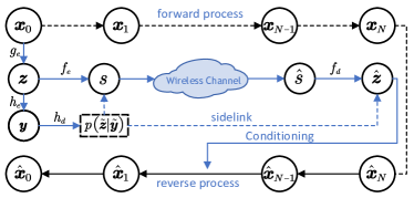
As illustrated in Fig. 1, the source image, represented by a pixel intensity vector , is first processed by a nonlinear transform coding encoder , producing a low-dimensional latent representation , where encompasses the trainable parameters. Inspired by [5], we estimate the distribution of , i.e., the quantized version of , by utilizing hyperprior entropy models. Specifically, we introduce an additional latent feature , serving as side information to capture the dependencies among the elements in , where represents the parametric analysis transform, and denotes its trainable parameters. Each in is variationally modeled as a Gaussian distribution with the standard deviation and mean predicted based on the quantized as:
| (1) |
where , is the parametric synthesis transform, denotes its trainable parameters, and represents the convolutional operation. Moreover, we convolve each element with a standard uniform density to enable a better match of the prior to the distribution of [5].
In this way, we are able to control the channel bandwidth ratio (CBR) based on the estimated entropy of . Specifically, comprises multiple embedding vectors of length . The JSCC encoder adjusts the length of each vector to , where denotes the quantization operation, controls the relation between the prior , and the expected length of the corresponding symbol vector . In particular, when the entropy of is high, a higher CBR is adopted, resulting in a larger . This process is expressed as where denotes the channel input symbols, is the number of transmitted symbols, and denotes the trainable parameters. Additionally, to meet the energy constraints of real-world communication systems, we ensure that satisfies an average power constraint before transmission.
Then, is transmitted through a noisy wireless channel, which is denoted by . As the additive white Gaussian noise (AWGN) channel is adopted in our work, this process follows , where is a complex Gaussian vector with variance . At the receiver, is first decoded to obtain the reconstructed latent , where represents the JSCC decoder, and denotes its trainable parameters. The receiver utilizes as an additional “content” latent to guide the conditional diffusion decoder to reconstruct images , where is the randomly sampled Gaussian source and represents the trainable parameters, as shown in Fig. 1. The details of the conditional diffusion decoder will be provided in the following section.

II-B Conditional Diffusion Decoder
We build our decoder on conditional diffusion models for their significant success in generative tasks.
The core idea of diffusion models is to transform an image into a Gaussian distribution by progressively adding noise to it, referred to as the forward process , resulting in a sequence of increasingly noisy versions . Then, the reverse process generates high-quality samples by reversing this process. The two Markov processes at step can be respectively described as follows:
| (2) |
| (3) |
where the variance is held constant as hyperparameters, the reverse process mean is parameterized by a neural network, and the variance is always set to .
The diffusion models are typically trained to predict the accumulated noise that perturbs to , a process known as -prediction, with the loss function being:
| (4) |
where , , , and .
In our conditional diffusion decoder, is taken as the condition for the reverse process. Consequently, the forward process remains unchanged as (2), and the reverse process is replaced by:
| (5) |
Analogous to (4), we modify the training objective as follows:
| (6) |
First, we employ -prediction [14] to predict the source image instead of using -prediction. -prediction requires only a few denoising steps yet achieves performance comparable to -prediction, which involves hundreds of denoising steps. This is because the optimization objective resembles an autoencoder loss, allowing the model to reconstruct the source image in a single iteration. Moreover, we replace the step with a normalized step , enabling the use of a smaller during testing compared to training, thereby accelerating the decoding process.
During inference, images are generated using ancestral sampling with Langevin dynamics as follows:
| (7) | ||||
III Training Strategy and Model Architecture
In this section, we first present the architecture of CDM-JSCC. Then, we analyze the proposed loss function. Finally, we propose a multi-stage training algorithm to ensure the stability and improve the overall performance.
III-A Model Architecture
As shown in Fig. 2, the proposed model consists of a transmitter, a wireless channel, and a receiver. We adopt the AWGN channel in our work, which is incorporated as a non-trainable layer in the architecture.
III-A1 Transmitter
The transmitter consists of an entropy encoder and a rate-adaptive JSCC encoder. The entropy encoder comprises a hyperprior model to effectively capture spatial dependencies in the latent representation [5]. The encoder consists of residual blocks followed by down-sampling convolution layers connected sequentially. The hyperprior encoder is composed of a down-sampling convolution layer followed by a ReLU activation function, while the hyperprior decoder is composed of an up-sampling convolution layer and a ReLU activation function. Then, is input to the JSCC encoder, where it is compressed into a variable-length latent representation based on the estimated entropy . Specifically, elements are selected and masked sequentially in a one-dimensional checkerboard pattern, which captures global features more effectively than random selection or linear sequencing. In addition, our proposed model is built on the advanced MLLA skeleton, known for its exceptional performance in image processing tasks and fast inference speed. The JSCC encoder consists of MLLA blocks and multiple multi-layer perceptrons (MLPs).
III-A2 Receiver
The receiver consists of a rate-adaptive JSCC decoder and a conditional diffusion decoder. The JSCC decoder inverts the operations performed by the JSCC encoder. Then, is input to the diffusion decoder as conditional information to guide the denoising process. The diffusion denoising unit is built on a U-Net architecture, featuring skip connections that allow the output from each down-sampling unit to be directly passed to the corresponding up-sampling unit. The architecture includes down-sampling units and up-sampling units, with a mid-block in between. Each down-sampling unit, up-sampling unit, and mid-block is composed of residual blocks and linear attention mechanisms. In addition, is encoded into features of different scales by layers of hierarchical encoders. These features are concatenated with the output of the preceding down-sampling unit and embed time information as input for the next down-sampling unit. During testing, the output is passed through the diffusion denoising unit iteratively until is produced.
III-B Loss Function
In a typical end-to-end JSCC system, the optimization focuses sorely on the MSE between the source image and the reconstructed image, with the loss function defined as:
| (8) |
which aligns with the training objective of our conditional diffusion models as defined in (8), with the exception that step and noise are randomly sampled.
Moreover, for an entropy model-based rate-adaptive JSCC system, the loss function is typically defined as:
| (9) | ||||
where is the compression distortion between the source image and the compressed image , represents the compression rate estimated by entropy models, and denotes the typical JSCC loss term.
To improve the perceptual quality of reconstructed images, we introduce an additional perceptual loss, expressed as follows:
| (10) |
where represents the perceptual loss term. Here we adopt widely-used learned perceptual image patch similarity (LPIPS) loss based on VGGNet [16]. Therefore, the objective for our model can be expressed as:
| (11) | ||||
where balances the trade-off between MSE distortion and the perceptual loss term, while adjusts the trade-off between the image quality and transmission rate.
III-C Training Strategy
To ensure training stability and enhance overall performance, we propose a multi-stage training strategy. Initially, we train each module individually to reduce complexity and facilitate convergence. Once all modules have been trained separately, we fine-tune the entire model to optimize performance. The complete multi-stage training process is detailed in Algorithm 1.
IV Simulation Results
In this section, we perform simulations to evaluate the performance of the proposed CDM-JSCC.
IV-A Simulation Settings
IV-A1 Basic Settings
We evaluate our CDM-JSCC on the Kodak image dataset, which consists of images, each with a resolution of . During testing, we only employ denoising steps at the receiver, ensuring an efficient and fast decoding process. All experiments are conducted using Pytorch. For the training process, we use the Adam optimizer for stochastic gradient descent, starting with a learning rate of and planning to reduce it after several epochs. The training dataset comprises randomly sampled images from the ImageNet dataset, which are randomly cropped to . The batch size is set to . We set and for the experiments.
IV-A2 Benchmarks
For benchmarks, we consider both deep learning-based methods and traditional separation-based schemes, incorporating optimization strategies for both MSE distortion and perceptual loss. The benchmarks are detailed as follows:
-
•
“BPG+LDPC”: This method employs BPG for source coding and LDPC for channel coding, followed by quadrature amplitude modulation (QAM).
-
•
“BPG+capacity”: In this approach, we use an ideal capacity-achieving channel coding in conjunction with BPG and QAM.
-
•
“DeepJSCC”: As a representative learning-based method, we include the classic DeepJSCC optimized for MSE distortion [2].
-
•
“GAN-JSCC”: This method optimizes both MSE distortion and perceptual loss [9].
IV-A3 Considered Metrics
We evaluate the performance of our method along with benchmarks using typical metric PSNR as well as perceptual metrics LPIPS[16], and Fréchet Inception Distance (FID). PSNR calculates pixel-wise MSE distortion. LPIPS measures the 2 distance between two latent embeddings extracted by a pre-trained network [16]. FID calculates the distribution of source images and reconstructed images in the feature space using the Fréchet distance [17].
IV-B Performance Comparison
We evaluate the performance of our proposed model on the AWGN channel, a representative and widely adopted method in this research community. In all subsequent experiments, the model is trained on a single SNR value and tested on the same SNR. In addition, by carefully adjusting the hyper-parameters, we control the CBR .
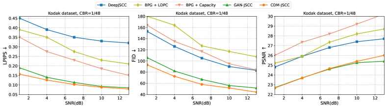
Fig. 3 compares CDM-JSCC with benchmarks across various SNRs, illustrating a comparative analysis of our proposed CDM-JSCC against the benchmarks. Notably, our model outperforms others across all perceptual quality metrics, including LPIPS and FID. This enhancement is attributed to the proposed loss function and the powerful generative diffusion models. However, it is important to note that our scheme shows some performance degradation in the PSNR metric compared to the MSE-optimized DeepJSCC and traditional separation-based schemes. This is because generative models tend to generate realistic and clear images and may overlook pixel-wise fidelity sometimes. Despite this, our model still outperforms GAN-JSCC in the PSNR metric. Unlike GAN-JSCC, our model does not plateau as SNR increases, maintaining the potential to transmit clear, realistic, and high-fidelity images at higher SNR levels.
V Conclusion
In this letter, we proposed a framework of conditional diffusion models-based generative DJSCC system for image transmission. Moreover, we employed -prediction with a few denoising steps to accelerate the decoding process. Furthermore, we effectively managed the transmission bandwidth based on the estimated entropy of transmitted symbols. Besides, we proposed a multi-state training strategy to ensure the stability of the training process. Simulation results demonstrated that the proposed method can significantly surpass existing methods in terms of perceptual quality.
References
- [1] C. You, Y. Cai, Y. Liu, M. Di Renzo, T. M. Duman, A. Yener, and A. L. Swindlehurst, “Next generation advanced transceiver technologies for 6G,” arXiv preprint arXiv:2403.16458, 2024.
- [2] E. Bourtsoulatze, D. Burth Kurka, and D. Gunduz, “Deep joint source-channel coding for wireless image transmission,” IEEE Trans. Cognit. Comm. Netw., vol. 5, no. 3, pp. 567–579, Sep. 2019.
- [3] H. Xie, Z. Qin, and G. Y. Li, “Task-oriented multi-user semantic communications for VQA,” IEEE Wireless Commun. Lett., vol. 11, no. 3, pp. 553–557, 2021.
- [4] H. Wu, Y. Shao, E. Ozfatura, K. Mikolajczyk, and D. Gündüz, “Transformer-aided wireless image transmission with channel feedback,” IEEE Trans. Wireless Commun., 2024.
- [5] J. Ballé, D. Minnen, S. Singh, S. J. Hwang, and N. Johnston, “Variational image compression with a scale hyperprior,” in Proc. Int. Conf. Learn. Represent. (ICLR), 2018.
- [6] J. Dai, S. Wang, K. Tan, Z. Si, X. Qin, K. Niu, and P. Zhang, “Nonlinear transform source-channel coding for semantic communications,” IEEE J. Select. Areas Commun., vol. 40, no. 8, pp. 2300–2316, 2022.
- [7] G. Zhang, P. Yang, Y. Cai, Q. Hu, and G. Yu, “From analog to digital: Multi-order digital joint coding-modulation for semantic communication,” arXiv preprint arXiv:2406.05437, 2024.
- [8] Y. Blau and T. Michaeli, “Rethinking lossy compression: The rate-distortion-perception tradeoff,” in Proc. Int. Conf. Mach. Learn. (ICML), 2019, pp. 675–685.
- [9] J. Wang, S. Wang, J. Dai, Z. Si, D. Zhou, and K. Niu, “Perceptual learned source-channel coding for high-fidelity image semantic transmission,” in Proc. IEEE Global Commun. Conf. (GLOBECOM), 2022, pp. 3959–3964.
- [10] A. Li, X. Liu, G. Wang, and P. Zhang, “Domain knowledge driven semantic communication for image transmission over wireless channels,” IEEE Wireless Commun. Lett., vol. 12, no. 1, pp. 55–59, 2022.
- [11] S. F. Yilmaz, X. Niu, B. Bai, W. Han, L. Deng, and D. Gündüz, “High perceptual quality wireless image delivery with denoising diffusion models,” in IEEE Conf. Comput. Commun. Workshops. (INFOCOM WKSHPS), 2024, pp. 1–5.
- [12] J. Ho, A. Jain, and P. Abbeel, “Denoising diffusion probabilistic models,” in Proc. Adv. Neural Inf. Process. Syst. (NIPS), 2020, pp. 6840–6851.
- [13] M. Yang, B. Liu, B. Wang, and H.-S. Kim, “Diffusion-aided joint source channel coding for high realism wireless image transmission,” arXiv preprint arXiv:2404.17736, 2024.
- [14] R. Yang and S. Mandt, “Lossy image compression with conditional diffusion models,” in Proc. Adv. Neural Inf. Process. Syst. (NIPS), vol. 36, 2024.
- [15] D. Han, Z. Wang, Z. Xia, Y. Han, Y. Pu, C. Ge, J. Song, S. Song, B. Zheng, and G. Huang, “Demystify mamba in vision: A linear attention perspective,” arXiv preprint arXiv:2405.16605, 2024.
- [16] R. Zhang, P. Isola, A. A. Efros, E. Shechtman, and O. Wang, “The unreasonable effectiveness of deep features as a perceptual metric,” in Proc. IEEE Conf. Comput. Vision Pattern Recognit. (CVPR), 2018, pp. 586–595.
- [17] M. Heusel, H. Ramsauer, T. Unterthiner, B. Nessler, and S. Hochreiter, “Gans trained by a two time-scale update rule converge to a local nash equilibrium,” in Proc. Adv. Neural Inf. Process. Syst. (NIPS), vol. 30, 2017.