Multiview Random Vector Functional Link Network for Predicting DNA-Binding Proteins

Abstract

The identification of DNA-binding proteins (DBPs) is a critical task due to their significant impact on various biological activities. Understanding the mechanisms underlying protein-DNA interactions is essential for elucidating various life activities. In recent years, machine learning-based models have been prominently utilized for DBP prediction. In this paper, to predict DBPs, we propose a novel framework termed a multiview random vector functional link (MvRVFL) network, which fuses neural network architecture with multiview learning. The proposed MvRVFL model combines the benefits of late and early fusion, allowing for distinct regularization parameters across different views while leveraging a closed-form solution to determine unknown parameters efficiently. The primal objective function incorporates a coupling term aimed at minimizing a composite of errors stemming from all views. From each of the three protein views of the DBP datasets, we extract five features. These features are then fused together by incorporating a hidden feature during the model training process. The performance of the proposed MvRVFL model on the DBP dataset surpasses that of baseline models, demonstrating its superior effectiveness. Furthermore, we extend our assessment to the UCI, KEEL, AwA, and Corel5k datasets, to establish the practicality of the proposed models. The consistency error bound, the generalization error bound, and empirical findings, coupled with rigorous statistical analyses, confirm the superior generalization capabilities of the MvRVFL model compared to the baseline models.

Keywords: Multiview learning, Support vector machine, Random vector functional link network, Extreme learning machine, DNA-binding protein.

1 Introduction

The protein capable of interacting with DNA is known as a DNA-binding protein (DBP) (Jones et al., 1987). The DBP plays a crucial role in numerous vital biological processes, including transcriptional regulation, DNA replication and repair, cellular development, and chromatin organization (Ohlendorf et al., 1982). Therefore, precise prediction of DBPs is of considerable significance for proteome annotation as well as endeavors in synthetic biology. To identify DBPs, extensive work has been carried out in wet lab settings, including techniques such as X-ray crystallography (Chou et al., 2003), genetic analysis (Freeman et al., 1995), and chromatin immunoprecipitation on microarrays (Buck & Lieb, 2004). While results obtained from wet-lab methods are likely the most reliable, it’s important to note that this approach is also associated with significantly high time and labor costs. In contrast to wet-lab methods, computational approaches can substantially decrease resource requirements and expedite the identification of DBPs. Furthermore, in the postgenomic era, there’s an escalating demand for the development of efficient and swift computational methods for accurately identifying DBPs, thereby underscoring its increasing significance in the field of bioinformatics.

Currently, computational methods are extensively employed for predicting DBPs (Qu et al., 2019). These methods are typically categorized into two groups: structure-based and sequence-based methods. Structure-based methods necessitate information obtained from the three-dimensional structure of the protein under examination. In the early stages, structure-based methods excelled in the domain of DBP prediction, exemplified by models like LBi-DBP (Zeng et al., 2024), StackDPP (Ahmed et al., 2024), DBPboost (Sun et al., 2024), and ULDNA (Zhu et al., 2024). Accurately representing a protein sequence as a vector is widely recognized as one of the sequence-based methods’ most essential and challenging tasks (Zhang & Liu, 2019). DNABinder (Ranjan et al., 2021) uses evolutionary information encoded in a position-specific scoring matrix (PSSM), generated via the PSI-BLAST multiple sequence alignment tool (Altschul et al., 1997a). A support vector machine (SVM) is employed for classification, using these features as input, marking the first instance of this approach being used to identify DNA-binding proteins (DBPs). In iDNA-Prot (Chou, 2011), pseudo amino acid composition (PseAAC) features (Chowdhury et al., 2017), extracted from protein sequences using the grey model, are amalgamated with random forest (RF) for the identification of DBPs. iDNAProt-ES (Chowdhury et al., 2017) utilizes evolutionary data like PSSM alongside structural information predicted by SPIDER2 (Yang et al., 2017) to characterize the features of a given protein. These features are trained to identify DBPs using SVM with a linear kernel. DBP datasets, derived from various sources or views, offer complementary information essential for improving task performance. Each view contributes unique perspectives and features that, when combined, enhance the overall understanding and efficiency of the model. Nevertheless, existing multiview learning approaches often necessitate complex architectures or extensive preprocessing to manage these diverse views effectively (Hu et al., 2023). The growing complexity of data from different sources poses significant challenges in extracting meaningful insights and achieving high performance. Multiview information fusion has gained widespread use in the field of bioinformatics in recent years (Zou et al., 2019; Zhou et al., 2022). The fuzzy kernel ridge regression model based on multi-view sequence features (FKRR-MVSF) (Zou et al., 2019) is proposed for identifying DNA-binding proteins. In FKRR-MVSF, the initial step is to extract multi-view sequence features from the protein sequences. Then, a multiple kernel learning (MKL) algorithm is used to combine these multiple features. In MSFBinder (Liu et al., 2018), a stacking framework is proposed to predict DBPs by combining features from multiple views. The multi-view hypergraph restricted kernel machines (MV-H-RKM) (Guan et al., 2022) model is proposed to extract multiple features from protein sequences. These features are connected via a common hidden feature, and multi-hypergraph regularization is applied to merge the multi-view features, maintaining structural consistency between the original and hidden features.

Despite the extensive use of hyperplane-based classifiers like SVMs and their variants in predicting DNA-binding proteins, a significant gap remains in exploring the potential of shallow neural networks for this task. Shallow neural networks, with their ability to learn complex data representations and capture non-linear relationships through hidden layers, present a compelling alternative to traditional machine learning models. However, conventional neural network models often face challenges like slow convergence, difficulties with local minima, and sensitivity to learning rates and initialization points, resulting in suboptimal outcomes. This challenge underscores the need for innovative yet simple approaches that can effectively manage diverse data types and leverage their full potential. At this juncture, the random vector functional link (RVFL) network emerges as a promising solution. Known for its simplicity and effectiveness across various machine learning tasks, RVFL can bridge the gap left by traditional neural networks.

Building on the previous discussion of MVL and the advantages of RVFL over conventional ANNs and ML models, we see a clear path forward in fusing these methods. The primary reason for this fusion is that the resulting model will be simple, scalable, efficient, and highly effective for DNA-binding protein prediction. Hence, we propose a novel multiview random vector functional link network (MvRVFL). MvRVFL adopts the framework of artificial neural networks combined with MVL, mirroring the structure of RVFL. To ensure the proposed model remains simple and effective, we incorporate two views at a time in the MvRVFL model. This approach strikes a balance between complexity and performance, leveraging complementary information from two views to enhance effectiveness while maintaining simplicity.
The following are the key features of the proposed MvRVFL model:

1. Integrating features from diverse perspectives enhances the proposed MvRVFL model’s capability to capture intricate patterns and relationships within the data, consequently enhancing the overall generalization performance of the model.

2. In the primary objective function of the proposed MvRVFL model, we encompass a coupling term, aiming to minimize a composite of errors originating from all views. By amalgamating the advantages of both early and late fusion, the model can assimilate information from all views during the training phase, yet still permits some flexibility to model the views distinctly.

3. The integration of multiple views in the proposed MvRVFL model helps to mitigate the impact of missing or noisy data in any single view (a common problem in biomedical datasets (Emmanuel et al., 2021)), thereby enhancing the model’s robustness and reliability.

The paper’s main highlights are as follows:

• We propose a novel multiview random vector functional link (MvRVFL) network. The proposed MvRVFL leverages multiple distinct feature sets using the MVL and the simplicity cum effectiveness of RVFL to predict DBP.

• We provide rigorous mathematical frameworks for MvRVFL, leveraging the RVFL topology. We utilized the Rademacher complexity theory to examine the consistency error bound and the generalization error bound of the proposed MvRVFL.

• Following (Guan et al., 2022), in this work, we partition each protein sequence into five equal-length segments, creating a total of 14 continuous or discontinuous regions. Each region is characterized using 63-dimensional features (7 + 21 + 35), leading to a comprehensive 882-dimensional (63 x 14) feature representation of the entire protein sequence. We extract five types of features from the sequences: NMBAC, MCD, PSSM-AB, PSSM-DWT, and PsePSSM. Experiments showcased that our method surpasses traditional models in effectively identifying DNA-binding proteins.

• Moreover, to test the generalization performance of the proposed model, we further tested it over the UCI, KEEL, AwA, and Corel5k datasets from various domains. The empirical results illustrate that the proposed MvRVFL model exhibits superior performance compared to numerous baseline models.

The remaining structure of the paper is organized as follows. We discuss the literature on the baseline model in Section 2. Section 3, provides an overview of related work. Section 4 covers the method for extracting features from DNA-binding protein sequences. We present the detailed mathematical formulation of the proposed MvRVFL model in Section 5. Experimental results and analyses of proposed and existing models are discussed in Section 6. Finally, Section 7 presents the conclusions and potential future research directions.

2 Background

In this section, we discuss the background of DNA-binding proteins, artificial neural networks, and multi-view learning in detail.

First, we explore the importance and function of DNA-binding proteins, which play a crucial role in various biological processes by interacting with DNA sequences. Next, we delve into the fundamentals of artificial neural networks (ANNs), a type of machine-learning model inspired by the human brain, and examine their architecture, learning mechanisms, and applications. Finally, we cover the concept of multi-view learning, a technique that integrates multiple sets of features or perspectives to improve the performance of the predictive model.

2.1 DNA binding protein

A DBP is a protein that can physically interact with DNA through its internal binding domain. As one of the most common intracellular proteins, DBPs play a crucial role in influencing genome function by participating in transcription, DNA replication, and DNA repair (Zimmermann et al., 2020). The active role of DBPs in cellular processes underscores their importance. As new proteins continue to be discovered in the post-genomic era, the identification of DBPs across various sequences has gained considerable attention. How can DBPs be identified among the multitude of newly discovered proteins? Experimental detection methods, which are resource-intensive, are not as cost-effective as computational approaches. As a result, recent years have seen the development of numerous computational predictive models for identifying DBPs. (Lin et al., 2011) introduced iDNA-Prot, which utilizes the pseudo amino acid composition (PseACC) (Fu et al., 2019) for feature extraction and applies a random forest (RF) classifier. Subsequently, Liu et al. developed three successive predictors: iDNA-Prot|dis (Liu et al., 2014), PseDNA-Pro (Liu et al., 2015c), and iDNAPro-PseAAC (Liu et al., 2015b). These predictors combined features from various extraction algorithms and used the integrated features as input for SVM to make predictions. Similarly, StackPDB predicts DNA-binding proteins through a three-step process: feature extraction, feature selection, and model construction are the key stages. StackPDB extracts features from protein sequences based on amino acid composition and evolutionary information. Evolutionary information is captured using the position-specific scoring matrix (PSSM), which is generated by the PSI-BLAST (Altschul et al., 1997b) program. In the StackPDB method, PsePSSM, PSSM-TPC, EDT, and RPT are employed for extracting features from PSSM. They subsequently used extreme gradient boosting combined with recursive feature elimination to select the most effective features. Finally, the selected optimal feature subset is input into a stacked ensemble classifier comprising XGBoost, SVM, and LightGBM. Previous studies (Ding et al., 2017; 2019) demonstrate that protein sequences can be characterized through different representations, including amino acid composition and PSSM. As fusion methods can combine information from multiple representations to improve model performance, various fusion techniques are employed in the identification of DBPs.

Multiple kernel learning (MKL) is a popular early fusion technique that focuses on learning the optimal weights for kernels. The optimal kernel is created by linearly combining multiple base kernels according to their respective weights. CKA-MKL (Qian et al., 2021) seeks to maximize the cosine similarity between the optimal kernel and the ideal kernel. Additionally, CKA-MKL includes a Laplacian term associated with the weights in the objective function to avoid extreme scenarios. However, CKA-MKL primarily emphasizes global kernel alignment and does not account for the differences between local samples. Therefore, HKAM-MKL (Zhao et al., 2022a) strives to maximize both local and global kernel alignment scores. Both CKA-MKL and HKAM-MKL utilize SVM as their classifier. In contrast, HSIC-MKL (Qian et al., 2022) aims to maximize the independence between trained samples and labels within the Reproducing Kernel Hilbert Space (RKHS). The optimal kernel is then used as input for a hypergraph-based Laplacian SVM, an extension of the standard SVM. In contrast, CKA-MKL focuses solely on global alignment. Moreover, HKAM-MKL takes into account both global and local aspects. As a result, HKAM-MKL outperforms CKA-MKL in predicting DNA-binding proteins. Unlike the previously mentioned MKL methods, MLapSVM-LBS (Sun et al., 2022) integrates multiple types of information throughout the training process. It uses the multiple local behavior similarity graph as a regularization term. Given that the objective function of MLapSVM-LBS is non-convex, an alternating algorithm is applied. The key advantage of MLapSVM-LBS is its ability to fuse various sources of information during training while providing flexibility to model different views distinctly.

2.2 Artificial neural networks

Artificial neural networks (ANNs) are a category of machine learning models inspired by the neural structure of the human brain. ANNs comprise interconnected nodes, or neurons, which employ mathematical operations to process and transmit information. ANNs are engineered to identify patterns and correlations within data, leveraging this acquired knowledge to make predictions. ANNs have showcased efficacy across diverse domains, including brain age prediction (Tanveer et al., 2023), fault diagnosis of drilling pumps (Guo et al., 2024), detection of sickle cell disease (Goswami et al., 2024), rainfall forecasting (Luk et al., 2001), diagnosis of Alzheimer’s disease (Tanveer et al., 2024; Ganaie et al., 2024), and so on. Conventional ANNs rely on gradient descent (GD) based iterative methods, which present several inherent challenges in parameter calculation. These include a tendency to converge to local rather than global optima, heightened sensitivity to the choice of learning rate and initial parameters, and a sluggish convergence rate.

To circumvent the limitations of GD-based neural networks, randomized neural network (RNN) (Schmidt et al., 1992) is proposed. In RNNs, certain network parameters remain fixed, with only the parameters of the output layer being computed using a closed-form solution throughout the training phase (Suganthan & Katuwal, 2021). The random vector functional link (RVFL) neural network (Pao et al., 1994; Malik et al., 2023) is a shallow feed-forward RNN distinguished by randomly initialized hidden layer parameters, which remain constant during the training process. RVFL stands out among other RNNs because of its direct connections between output and input layers. These direct links serve as a type of implicit regularization (Zhang & Suganthan, 2016; Sajid et al., 2024) within RVFL, contributing to enhanced learning capabilities. Through methods such as the least-squares technique or Pseudo-inverse, RVFL provides a closed-form solution for optimizing output parameters. This characteristic leads to efficient learning with fewer adjustable parameters. For more details, interested readers can refer to the comprehensive review paper of RVFL (Malik et al., 2023).

2.3 Multiview learning

Multiview learning (MVL), as a prominent research field, showcases the ability to substantially improve generalization performance across diverse learning tasks by integrating multiple feature sets that encompass complementary information (Zhao et al., 2017b; Xu et al., 2017; Tang et al., 2020). MVL emerges in response to the common occurrence of diverse types of data in practical scenarios. Consider an image, which can be characterized by its color or texture features, and a person, who can be identified through facial characteristics or fingerprints. In real-world situations, samples from different perspectives might exist in separate spaces or display notably different distributions because of the significant variation between views. However, the naive methods address this data type by employing a cascade strategy (Xu et al., 2017). This entails transforming the multiview data into new single-view data by consolidating the heterogeneous feature space into a homogeneous feature space. However, the cascading strategy overlooks the unique statistical properties of each view and is plagued by the curse of dimensionality. MVL techniques (Tang et al., 2019; Huang et al., 2020) are applied across various tasks, including transfer learning (Zhao et al., 2017a), clustering (Wen et al., 2018; 2020), dimensionality reduction (Wang & Zhang, 2013; Hu et al., 2019), and classification (Sun et al., 2018). SVM-2K, a two-view SVM learning model that combines SVMs with the kernel canonical correlation analysis (KCCA) distance minimization version, was first introduced by (Farquhar et al., 2005). Using the consensus principle, this method makes use of two points of view. Multiview twin SVM (MvTSVM) (Xie & Sun, 2015) represents the initial endeavor to integrate a best-fitting hyperplane classifier with MVL. In recent years, various variants of MvTSVM have been introduced such as multiview one-class SVM method with LUPI (MOCPIL) (Xiao et al., 2024), multiview large margin distribution machine (MVLDM) (Hu et al., 2024), multiview restricted kernel machine (MVRKM) (Houthuys & Suykens, 2021), and multiview robust double-sided TSVM (MvRDTSVM) (Ye et al., 2021).

3 Related Work

This section begins with establishing notations and then reviews the mathematical formulation along with the solution of the RVFL network.

3.1 Notations

Consider the sample space denoted as $\mathscr{T}$, which is a product of two distinct feature views, $A$ and $B$, expressed as $\mathscr{T}=\mathscr{T}^{A}\times\mathscr{T}^{B}$, where $\mathscr{T}^{A}\subseteq\mathbb{R}^{m_{1}}$, $\mathscr{T}^{B}\subseteq\mathbb{R}^{m_{2}}$ and $\mathscr{Y}=\{-1,+1\}$ denotes the label space. Here $n$ represents the number of samples, $m_{1}$ and $m_{2}$ denote the number of features corresponding to view $A$ (Vw-$A$) and view $B$ (Vw-$B$), respectively. Suppose $\mathscr{H}=\{(x_{i}^{A},x_{i}^{B},y_{i})|x_{i}^{A}\in\mathscr{T}^{A},x_{i}^{B}\in\mathscr{T}^{B},y_{i}\in\mathscr{Y}\}_{i=1}^{n}$ represent a two-view dataset. Let $X_{1}\subseteq\mathbb{R}^{n\times m_{1}}$ and $X_{2}\subseteq\mathbb{R}^{n\times m_{2}}$ be the input matrix of Vw-$A$ and Vw-$B$, respectively and one-hot encoding matrix of the labels is denoted by $Y\subseteq\mathbb{R}^{n\times 2}$. $Z_{1}\subseteq\mathbb{R}^{n\times h_{l}}$ and $Z_{2}\subseteq\mathbb{R}^{n\times h_{l}}$ are hidden layer matrices, which are obtained by applying a nonlinear activation function, denoted as $\phi$, to the input matrices $X_{1}$ and $X_{2}$ after transforming them with randomly initialized weights and biases. Here $h_{l}$ represents the number of hidden layer nodes and $(.)^{t}$ represents the transpose operator.

3.2 Random Vector Functional Link (RVFL) Network

The RVFL (Pao et al., 1994) is a single-layer feed-forward neural network composed of three layers: the input layer, the hidden layer, and the output layer. The weights connecting the input and hidden layers, as well as the biases in the hidden layer, are randomly initialized and remain unchanged during the training process. The original features of input samples are also directly connected to the output layer. The determination of output layer weights involves analytical techniques such as the least square method or the Moore-Penrose inverse. The architecture of the RVFL model is shown in Fig. 1.

Figure 1: Geometrical structure of RVFL model

Consider $T=\{(x_{i},y_{i}),i=1,2,\ldots,n\}$ be the training dataset, where $y_{i}\in\{+1,-1\}$ represents the label of $x_{i}\in\mathbb{R}^{1\times m}$. Let $X=(x_{1}^{t},x_{2}^{t},\ldots,x_{n}^{t})^{t}\in\mathbb{R}^{n\times m}$ and $Y=(y_{1}^{t},y_{2}^{t},\ldots,y_{n}^{t})^{t}\in\mathbb{R}^{n\times 2}$ be the collection of all input and target vectors, respectively. $H_{1}$ is the hidden layer matrix, acquired by projecting the input matrix using randomly initialized weights and biases and then subjecting it to the non-linear activation function $\phi$. It is defined as:

$$H_{1}=\phi(XW_{1}+b_{1})\in\mathbb{R}^{n\times h_{l}},$$ (1)

where $W_{1}\in\mathbb{R}^{m\times h_{l}}$ represents the weights vector which is initialized randomly, and drawn from a uniform distribution spanning $[-1,1]$, and $b_{1}\in\mathbb{R}^{n\times h_{l}}$ is the bias matrix. Thus, $H_{1}$ is given as:

$$H_{1}=\begin{bmatrix}\phi(x_{1}w_{1}+b^{(1)})&\ldots&\phi(x_{1}w_{h_{l}}+b^{(h_{l})})\\ \vdots&\vdots&\vdots\\ \phi(x_{n}w_{n}+b^{(1)})&\ldots&\phi(x_{n}w_{h_{l}}+b^{(h_{l})})\end{bmatrix},$$ (2)

here $w_{k}\in\mathbb{R}^{m\times 1}$ represents the $k^{th}$ column vector of the weights matrix of $W_{1}$, $x_{i}\in\mathbb{R}^{1\times m}$ denotes the $i^{th}$ sample of matrix $X$ and $b^{(j)}$ signifies the bias term of the $j^{th}$ hidden node. The weights of the output layer are determined through the following matrix equation:

$$\begin{bmatrix}X&H_{1}\end{bmatrix}W_{2}=\hat{Y}.$$ (3)

Here, $W_{2}\in\mathbb{R}^{(m+h_{l})\times 2}$ denotes the weights matrix, which connects the input with the concatenation of the hidden nodes to the output nodes, while $\hat{Y}$ represents the predicted output. The resulting optimization problem of Eq. (3) is formulated as:

$$(W_{2})_{min}=\underset{W_{2}}{\arg\min}\frac{\mathcal{C}}{2}\|H_{2}W_{2}-Y\|^{2}+\frac{1}{2}\|W_{2}\|^{2},$$ (4)

where $H_{2}=\begin{bmatrix}X&H_{1}\end{bmatrix}$. The optimal solution of Eq. (4) is defined as follows:

$$(W_{2})_{min}=\left\{\begin{array}[]{ll}\left({H_{2}}^{t}{H_{2}}+\frac{1}{\mathcal{C}}I\right)^{-1}{H_{2}}^{t}{Y},&(m+h_{l})\leq n,\vspace{3mm}\\ {H_{2}}^{t}\left({H_{2}}{H_{2}}^{t}+\frac{1}{\mathcal{C}}I\right)^{-1}{Y},&n<(m+h_{l}),\end{array}\right.$$ (7)

where $\mathcal{C}>0$ is a tunable parameter and $I$ represents the identity matrix of conformal dimensions.

4 Data Preprocessing and Feature Extractions

In this section, we begin by outlining the DBP sequence from three distinct perspectives. Next, we utilize five different algorithms to extract features from these perspectives (Guan et al., 2022). Finally, we use MvRVFL to combine these features and develop the predictor for identifying DBPs. Figure 2 illustrates the flowchart of the model construction process.

Figure 2: Flowchart of extracting features of Protein Sequences.

4.1 Features of DBP

In this subsection, we detail the DBP sequence from three different perspectives: physicochemical properties, evolutionary information, and amino acid composition. These views are transformed into feature matrices using various extraction algorithms: Multi-scale Continuous and Discontinuous (MCD) (You et al., 2014) for amino acid composition; Normalized Moreau-Broto Autocorrelation (NMBAC) (Ding et al., 2016) for physicochemical properties; and Pseudo Position-Specific Scoring Matrix (PsePSSM) (Liu et al., 2015a), PSSM-based Discrete Wavelet Transform (PSSM-DWT) (Nanni et al., 2012), and PSSM-based Average Blocks (PSSM-AB) (cheol Jeong et al., 2010), for evolutionary information.

4.2 Multi-Scale Continuous and Discontinuous for Protein Sequences

Multi-scale Continuous and Discontinuous (MCD) uses multi-scale decomposition techniques to first segment the protein sequence into equal-length sections, followed by the characterization of each continuous and discontinuous region. Three descriptors are used for each region: distribution (D), composition (C), and transition (T). The following outlines the detailed process of feature extraction for each descriptor.

For distribution (D), the protein sequence is categorized into 7 different types of amino acids. The total count of amino acid occurrences in each category is represented by $M_{i},\leavevmode\nobreak\ i\in\{1,2,\ldots,7\}$. Subsequently, within each amino acid category, we determine the positions of the $1^{st}$, $25^{th}$ percentile, $50^{th}$ percentile, $75^{th}$ percentile, and last amino acids of that category in the entire protein sequence. These positions are then normalized by dividing by the total sequence length $L$. Therefore, each amino acid category can be represented by a $5$-dimensional feature vector. For the entire protein sequence, this results in a $35$-dimensional feature vector.

For composition (C), the 20 standard amino acids are grouped into seven categories based on the dipoles and volumes of their side chains, with each group sharing similar characteristics. Table 1 provides a detailed list of the amino acids in each category. Let $S=\{s_{1},s_{2},\ldots,s_{L}\}$ denotes a protein sequence, where $s_{i}$ represents the $i^{th}$ residue and $L$ is the total length of the sequence. Based on Table 1, we can represent $S$ as $S=\{s_{1},s_{2},\ldots,s_{L}\}$, where each residue $s_{i}$ is classified into one of the categories $\{1,2,3,\ldots,7\}$. We then calculate the proportion of residues in each category throughout the entire protein sequence. For composition (C), it is represented as a 7-dimensional vector, where each dimension corresponds to one of the seven amino acid categories.

Table 1: Amino Acid Categories Based on Side Chain Dipoles and Volumes

Group 1	Group 2	Group 3	Group 4	Group 5	Group 6	Group 7
A, G, V	D, E	F, P, I, L	H, Q, N, W	K, R	T, Y, M, S	C

For transition (T), the entire protein sequence is divided into seven groups of amino acids according to the previously defined classification. We can calculate the frequency of transitions between different amino acid categories, which will be used to characterize the transition (T) properties of the protein. For transition (T), it can be represented as a $21$-dimensional vector, accounting for all possible transformations between the seven amino acid categories.

In this study, each protein sequence is partitioned into $5$ uniform-length segments, creating a total of 14 continuous or discontinuous regions. Each region is characterized by the $63$-dimensional features mentioned earlier ($7$ for composition, $21$ for transition, and $35$ for distribution). Consequently, the entire protein sequence is described using an $882$-dimensional feature vector ($63\times 14$).

Table 2: Six Physicochemical Properties Associated with Each Amino Acid

Amino acid	Q1	Q2	SASA	H	NCISC	VSC
D	0.105	13	1.587	-0.9	-0.02382	40
C	0.128	5.5	1.461	0.29	-0.03661	44.6
A	0.046	8.1	1.181	0.62	0.007187	27.5
R	0.291	10.5	2.56	-2.53	0.043587	105
G	0	9	0.881	0.48	0.179052	0
H	0.23	10.4	2.025	-0.4	-0.01069	79
P	0.131	8	1.468	0.12	0.239531	41.9
E	0.151	12.3	1.862	-0.74	0.006802	62
I	0.186	5.2	1.81	1.38	0.021631	93.5
N	0.134	11.6	1.655	-0.78	0.005392	58.7
Q	0.18	10.5	1.932	-0.85	0.049211	80.7
F	0.29	5.2	2.228	1.19	0.037552	115.5
L	0.186	4.9	1.931	1.06	0.051672	93.5
T	0.108	8.6	1.525	-0.05	0.003352	51.3
Y	0.298	6.2	2.368	0.26	0.023599	117.3
M	0.221	5.7	2.034	0.64	0.002683	94.1
W	0.409	5.4	2.663	0.81	0.037977	145.5
S	0.062	9.2	1.298	-0.18	0.004627	29.3
K	0.219	11.3	2.258	-1.5	0.017708	100
V	0.14	5.9	1.645	1.08	0.057004	71.5

4.3 Normalized Moreau-Broto Autocorrelation for Protein Sequences

Normalized Moreau-Broto Autocorrelation (NMBAC) is a feature based on the physicochemical properties of amino acids. We use the same approach (Ding et al., 2016) to extract features from protein sequences. In this study, six physicochemical properties of amino acids are taken into account: hydrophobicity (H), solvent accessible surface area (SASA), polarizability (P1), polarity (P2), volume of side chains (VSC), and net charge index of side chains (NCISC). The values for these six physicochemical properties for each amino acid are listed in Table 2. We normalize these values for each physicochemical property using the following formula:

$$\hat{M}_{i,j}=\frac{M_{i,j}-M_{j}}{S_{j}},$$ (8)

where $M_{i,j}$ represents the value of the $i^{th}$ amino acid for physicochemical property $j$, and $M_{j}$ is the mean value of the $20$ amino acids for property $j$. $S_{j}$ is the standard deviation of the physicochemical property $j$ among the $20$ amino acids. Hence, NMBAC can be computed using the following formula:

$$P(lg,j)=\frac{1}{L-lg}\sum_{i=1}^{L-lg}(\hat{M}_{i,j}\times\hat{M}_{{i+lg},j}),$$ (9)

where $j\in\{1,2,\ldots,6\}$ represents one of the six physicochemical properties, $i\in\{1,2,\ldots,20\}$ denotes the $i^{th}$ amino acid in the protein sequence, $L$ is the length of the protein sequence, and $lg$ is the distance between residues. We use the same $lg$ values as those in (Ding et al., 2016), ranging from $1$ to $30$. Consequently, this results in a $180$-dimensional vector $(30\times 6)$. Furthermore, we incorporate the frequency of the $20$ amino acids found in the protein sequence into the NMBAC feature. As a result, the final NMBAC feature vector is $200$-dimensional $(180+20)$.

Figure 3: Four-level discrete wavelet transform for PSSM analysis.

4.4 PSSM-Based Average Blocks for Protein Sequences

As PSSM includes evolutionary information about proteins, it has become a popular tool for various protein function prediction tasks in recent years. In this study, we extracted three features from PSSM: Pseudo Position-Specific Scoring Matrix (PsePSSM), PSSM-based Discrete Wavelet Transform (PSSM-DWT), and PSSM-based Average Blocks (PSSM-AB). The original PSSM profile, denoted as $Q_{PSSM}$, is represented as:

$$Q_{PSSM}=\begin{bmatrix}Q_{1,1}&Q_{1,2}&\cdots&Q_{1,20}\\ \vdots&\vdots&\ddots&\vdots\\ Q_{L,1}&Q_{L,2}&\cdots&Q_{L,20}\\ \end{bmatrix}_{L\times 20},$$ (10)

where $Q_{i,j}$ represents the score for the transition from the $i^{th}$ residue to the $j^{th}$ residue class throughout the evolutionary process. For every protein, the PSSM feature’s dimensionality is $L\times 20$.

The PSSM is initially divided into segments by PSSM-AB, where each block covers $5\%$ of the protein sequence. Consequently, the PSSM is divided into $20$ fundamental blocks, each of which consists of $20$ columns, independent of the length of the protein. The formula for extraction is as follows:

$$E_{j}=\frac{1}{A_{j}}\sum_{i=1}^{A_{j}}Q_{i}^{(j)},$$ (11)

where $E_{j}$ represents the feature vector of the $j^{th}$ block, with a dimension of $1\times 20$. The sequence length of the $j^{th}$ block is represented by $A_{j}$, and the PSSM value for the $i^{th}$ residue in the $j^{th}$ block, which also has a dimension of $1\times 20$, is indicated by $Q_{i}^{(j)}$. The feature vector derived from each protein sequence has a dimension of $400$ $(20\times 20)$, with a total of $20$ blocks.

4.5 PSSM-Based Discrete Wavelet Transform for Protein Sequences

We apply the Discrete Wavelet Transform (DWT) to extract features from the PSSM, referred to as PSSM-based DWT (PSSM-DWT). In this feature extraction method, each column of the PSSM profile of the protein serves as the input signal. Following the approach in (Ding et al., 2016), we apply a $4$-level discrete wavelet transform for analyzing the PSSM, as illustrated in Fig 3.

We use high-pass and low-pass filters to break down the approximation function at each step of the process, followed by downsampling. For every level, this method yields low-frequency coefficients $L_{i}$ and high-frequency coefficients $H_{i}$, where $i$ denotes the $i^{th}$ layer. We calculate the mean, median, maximum, and minimum values for both the low-frequency and high-frequency coefficients at each layer. Furthermore, we extract additional specific information from each layer of the low-frequency component by extracting the first five discrete cosine coefficients. Thus, for a protein’s PSSM profile, we obtain a $1040$-dimensional feature vector $((4+4+5)\times 4\times 20)$.

4.6 Pseudo PSSM for Protein Sequences

The dimensions of the PSSM features vary depending on the length of the protein sequence. When extracting features from the PSSM profile, the PsePSSM is often used to ensure that PSSM features have uniform dimensions and include sequence order information. The features derived from PsePSSM are organized as follows:

$$Q_{PsePSSM}=[Q_{1}\leavevmode\nobreak\ Q_{2}\leavevmode\nobreak\ \ldots Q_{20}\leavevmode\nobreak\ J_{1}^{\zeta_{1}}\leavevmode\nobreak\ J_{2}^{\zeta_{1}}\leavevmode\nobreak\ \ldots\leavevmode\nobreak\ J_{20}^{\zeta_{1}}\leavevmode\nobreak\ \ldots\leavevmode\nobreak\ J_{1}^{\zeta_{N}}\leavevmode\nobreak\ J_{2}^{\zeta_{N}}\leavevmode\nobreak\ \ldots\leavevmode\nobreak\ J_{20}^{\zeta_{N}}]^{T},$$ (12)

where

$$Q_{j}=\frac{1}{L}\sum_{i=1}^{L}Q_{i,j},\leavevmode\nobreak\ \leavevmode\nobreak\ j=1,2,\ldots,20,$$ (13)

and

$$J_{j}^{\zeta_{l}}=\frac{1}{L-\zeta_{l}}\sum_{i=1}^{L-\zeta_{l}}[Q_{i,j}-Q_{(i+\zeta_{l}),j}]^{2},\leavevmode\nobreak\ \leavevmode\nobreak\ \leavevmode\nobreak\ \zeta_{l}<L;\leavevmode\nobreak\ 1\leq l\leq N,$$ (14)

where $L$ denotes the length of the protein sequence, $l$ represents the distance between residues, $Q_{j}$ indicates the average score of residues in the protein sequence that evolve into the $j^{th}$ residue, and $J_{j}^{\zeta_{l}}$ reflects the PSSM scores for two residues that are adjacent with a distance of $l$. We adopt the same range of $l$ values as those used in (Chou & Shen, 2007), where $l$ varies from 1 to $15$. Thus, for a protein sequence, we generate a $320$-dimensional vector $(20+20\times 15)$. We can extract PSSM features with a fixed length using this technique while preserving sequence order information.

4.7 Feature Selection for Protein Sequences

In this section, we discuss feature selection and our use of the Minimum Redundancy–Maximum Relevancy (mRMR) method (Wei et al., 2017). This approach ranks the importance of input features by minimizing redundancy among them and maximizing their relevance to the target. In mRMR, mutual information is utilized to compute the redundancy and relevance mentioned above. The calculations are performed as follows:

$$J(g,h)=\iint p(g,h)\log\frac{p(g,h)}{p(g)p(h)}dg\leavevmode\nobreak\ dh,$$ (15)

where $g$ and $h$ are two vectors, $p(g)$ and $p(h)$ represent the marginal probability densities of $g$ and $h$ respectively, and $p(g,h)$ denotes the joint probability density of $g$ and $h$. We use $T$ to denote the full set of features, $T_{t}$ to represent a sorted subset with $m$ features, and $T_{n}$ to indicate an unsorted subset with $n$ features. Thus, the relevance $L$ and redundancy $D$ of features $k$ within the subset $T_{n}$ are calculated as follows:

$$L(k)=J(k,s),$$ (16)

$$D(k)=\frac{1}{m}\sum_{k_{i}\in T_{t}}J(k,k_{i}),$$ (17)

where $s$ represents the target associated with feature $k$. To maximize the relevance $L$ and minimize the redundancy $D$, we derive:

$$\underset{k_{i}\in T_{n}}{\min}[D(k_{i})-L(k_{i})],\leavevmode\nobreak\ \leavevmode\nobreak\ \leavevmode\nobreak\ i=1,2,3,\ldots,n.$$ (18)

By applying mRMR, we generate a reordered set of features, with each feature ranked according to its importance. For each feature, we subsequently select the optimal subset to be used in further experiments. Among the five feature types used in this paper, we first ranked the importance of features within each type using mRMR. Among the five feature types examined in this paper, we first ranked the importance of features within each category using mRMR. We then selected the top $1/2$, $3/4$, $7/8$, and $15/16$ of the features from the ranked list to form new feature subsets, respectively.

5 Proposed Multiview Random Vector Functional Link (MvRVFL) Network

This section offers an in-depth explanation of the proposed MvRVFL model. Initially, we outline the generic mathematical framework of the proposed MvRVFL model, specifically tailored to handle data originating from two distinct views. During training on one view, the influence of other views is incorporated by introducing a coupling term into the primal form of the proposed optimization problem. An intuitive illustration of the MvRVFL model is shown in Fig. 4. Let $Z_{1}$ and $Z_{2}$ represent the nonlinear projection of the class samples corresponding to Vw-$A$ and Vw-$B$, as defined by: $Z_{1}=[X_{1}\hskip 5.69046ptH_{1}]$ and $Z_{2}=[X_{2}\hskip 5.69046ptH_{2}]$. Here $X_{1}$ and $X_{2}$ represent the input matrix corresponding to Vw-$A$ and Vw-$B$, and $H_{1}$ and $H_{2}$ denote the hidden layer matrix corresponding to Vw-$A$ and Vw-$B$, respectively. These matrices are obtained by transforming $X_{1}$ and $X_{2}$ using randomly initialized weights and biases and then applying a nonlinear activation function. The target matrix is denoted by $Y$. The proposed optimization problem of MvRVFL model is articulated as follows:

$$\underset{\beta_{1},\beta_{2}}{\min}\hskip 5.69046pt \frac{1}{2}\|\beta_{1}\|^{2}+\frac{\theta}{2}\|\beta_{2}\|^{2}+\frac{\mathcal{C}_{1}}{2}\|\xi_{1}\|^{2}+\frac{\mathcal{C}_{2}}{2}\|\xi_{2}\|^{2}+\rho\xi_{1}^{t}\xi_{2}$$

s.t. $$Z_{1}\beta_{1}-Y=\xi_{1},$$

$$Z_{2}\beta_{2}-Y=\xi_{2}.$$ (19)

Figure 4: An intuitive illustration of MvRVFL model in two-view setting.

Here, $\beta_{1}$ and $\beta_{2}$ are the output weight matrix corresponding to Vw-$A$ and Vw-$B$, $\xi_{1}$ and $\xi_{2}$ represent the error corresponding to Vw-$A$ and Vw-$B$, respectively. $\mathcal{C}_{1}$, $\mathcal{C}_{2}$, $\theta$ and $\rho$ are the regularization parameters.

Each component of the optimization problem of MvRVFL has the following significance.

1. The terms $\|\beta_{1}\|$ and $\|\beta_{2}\|$ are regularization components for Vw-$A$ and Vw-$B$, respectively. These terms are employed to mitigate overfitting by constraining the capacities of the classifier sets for both views.

2. The error variables $\xi_{1}$ and $\xi_{2}$ are pertinent to both views, enabling tolerance for misclassifications in situations of overlapping distributions.

3. The primal optimization function comprises two distinct classification objectives for each view, linked by the coupling term $\rho\xi_{1}^{t}\xi_{2}$. Here, $\rho$ represents an additional regularization constant, referred to as the coupling parameter. This term serves to minimize the product of the error variables for both views as well as trade-off parameters between both views.

The Lagrangian corresponding to the problem Eq. (5) is given by

$$L= \frac{1}{2}\|\beta_{1}\|^{2}+\frac{\theta}{2}\|\beta_{2}\|^{2}+\frac{\mathcal{C}_{1}}{2}\|\xi_{1}\|^{2}+\frac{\mathcal{C}_{2}}{2}\|\xi_{2}\|^{2}+\rho\xi_{1}^{t}\xi_{2}-\alpha_{1}^{t}(Z_{1}\beta_{1}-Y-\xi_{1})-\alpha_{2}^{t}(Z_{2}\beta_{2}-Y-\xi_{2}),$$ (20)

where $\alpha_{1}\in\mathbb{R}^{n\times 1}$ and $\alpha_{2}\in\mathbb{R}^{n\times 1}$ are the vectors of Lagrangian multipliers.
Using the Karush-Kuhn-Tucker (K.K.T.) conditions, we have

$$\beta_{1}-Z_{1}^{t}\alpha_{1}=0,$$ (21)

$$\theta\beta_{2}-Z_{2}^{t}\alpha_{2}=0,$$ (22)

$$\mathcal{C}_{1}\xi_{1}+\rho\xi_{2}+\alpha_{1}=0,$$ (23)

$$\mathcal{C}_{2}\xi_{2}+\rho\xi_{1}+\alpha_{2}=0,$$ (24)

$$Z_{1}\beta_{1}-Y-\xi_{1}=0,$$ (25)

$$Z_{2}\beta_{2}-Y-\xi_{2}=0.$$ (26)

Using Eqs. (23), (25) and ( 26) in Eq. (21), we get

$$\beta_{1}=Z_{1}^{t}\alpha_{1},$$

$$\beta_{1}=-Z_{1}^{t}(\mathcal{C}_{1}\xi_{1}+\rho\xi_{2}),$$

$$\beta_{1}=-Z_{1}^{t}(\mathcal{C}_{1}(Z_{1}\beta_{1}-Y)+\rho(Z_{2}\beta_{2}-Y)),$$

$$(I+\mathcal{C}_{1}Z_{1}^{t}Z_{1})\beta_{1}+\rho Z_{1}^{t}Z_{2}\beta_{2}=Z_{1}^{t}(\mathcal{C}_{1}+\rho)Y.$$ (27)

Using Eqs. (24), (25) and (26) in Eq. (22), we get

$$\rho Z_{2}^{t}Z_{1}\beta_{1}+(\theta I+\mathcal{C}_{2}Z_{2}^{t}Z_{2})\beta_{2}=Z_{2}^{t}(\mathcal{C}_{2}+\rho)Y.$$ (28)

Using Eqs. (27) and (28), the solution of Eq. (5) is given by

$$\begin{bmatrix}\beta_{1}\\ \beta_{2}\end{bmatrix}=\begin{bmatrix}(I+\mathcal{C}_{1}Z_{1}^{t}Z_{1})&\rho Z_{1}^{t}Z_{2}\\ \rho Z_{2}^{t}Z_{1}&(\theta I+\mathcal{C}_{2}Z_{2}^{t}Z_{2})\\ \end{bmatrix}^{-1}\begin{bmatrix}Z_{1}^{t}(\mathcal{C}_{1}+\rho)\\ Z_{2}^{t}(\mathcal{C}_{2}+\rho)\end{bmatrix}Y.$$ (29)

After computing the optimal values of $\beta_{1}$ and $\beta_{2}$, the classification of a new input data point $x$ into either the $+1$ or $-1$ class can be determined as follows:

1. Firstly, the decision function of Vw-$A$ and Vw-$B$ can be articulated as follows:

   $$class^{A}(x^{A})=\underset{i\in\{1,2\}}{\arg\max}\{y_{A_{i}}\},$$ (30)

   $$\text{where}\hskip 5.69046pty_{A}=[x^{A}\hskip 5.69046pt\phi(x^{A}W^{A}+b^{A})]\beta_{1}\hskip 2.84544pt\text{and}\hskip 2.84544pty_{A}=(y_{A_{1}},y_{A_{2}})$$

   and

   $$class^{B}(x^{B})=\underset{i\in\{1,2\}}{\arg\max}\{y_{B_{i}}\},$$ (31)

   $$\text{where}\hskip 5.69046pty_{B}=[x^{B}\hskip 5.69046pt\phi(x^{B}W^{B}+b^{B})]\beta_{2}\hskip 2.84544pt\text{and}\hskip 2.84544pty_{B}=(y_{B_{1}},y_{B_{2}}).$$

2. The decision function, which combines two views, can be articulated in the following manner:

   $$class(x)=\underset{i\in\{1,2\}}{\arg\max}\{y_{c_{i}}\},$$ (32)

   where

   $$y_{c}=\frac{1}{2}\left([x^{A}\hskip 5.69046pt\phi(x^{A}W^{A}+b^{A})]\beta_{1}+[x^{B}\hskip 5.69046pt\phi(x^{B}W^{B}+b^{B})]\beta_{2}\right)\hskip 2.84544pt\text{and}\hskip 2.84544pty_{c}=(y_{c_{1}},y_{c_{2}}).$$

Here, $W^{A}$ ($W^{B}$) and $b^{A}$ ($b^{B}$) are the randomly generated weights and biases corresponding to Vw-$A$ (Vw-$B$), respectively.

Remark: The proposed MvRVFL model is referred to as MvRVFL-1 if the classification of the test sample is determined by the functions outlined in Eq. (32). Also, we employ majority voting to determine the final anticipated output of the proposed MvRVFL model by aggregating predictions from Eqs. (30), (31) and (32), and we refer to it as MvRVFL-2 model. In the majority voting technique, the class label with the highest number of votes is selected as the final prediction.

The algorithm of the proposed MvTPSVM model is briefly described in Algorithm 1. Furthermore, evaluating the generalization performance of MvRVFL requires a theoretical examination of its generalization error. To achieve this, we apply Rademacher’s complexity theory. In the Appendix (Section A.1), we delve into the consistency error bound and the generalization error bound of the MvRVFL model.

5.1 Complexity Analysis of the Proposed MvRVFL Model

Let $(X_{1},X_{2},Y)$ denote the training set, where $X_{1}\in\mathbb{R}^{n\times m_{1}}$, $X_{2}\in\mathbb{R}^{n\times m_{2}}$ and $Y\in\mathbb{R}^{n\times 2}$. Here, $m_{1}$ and $m_{2}$ denote the number of features corresponding to Vw-$A$ and Vw-$B$ and $n$ represents the number of samples, respectively. In RVFL-based models, the complexity is governed by the necessity to compute matrix inverses for optimizing the output layer weights. Thus, the size of the matrices requiring inversion dictates the model’s complexity. Therefore, the time complexity of the RVFL model is $\mathcal{O}(n^{3})$ or $\mathcal{O}((m+h_{l})^{3})$, where $h_{l}$ represents the number of hidden nodes. Hence, the proposed MvRVFL model is required to inverse the matrix of dimension $(m_{1}+m_{2}+2h_{l})\times(m_{1}+m_{2}+2h_{l})$. Therefore, the time complexity of the MvRVFL model is $\mathcal{O}((m_{1}+m_{2}+2h_{l})^{3})$.

Algorithm 1 MvRVFL classifier

Require: $X_{1}\in\mathbb{R}^{n\times m_{1}}$ and $X_{2}\in\mathbb{R}^{n\times m_{2}}$ be the input matrix of Vw-$A$ and Vw-$B$, respectively and $Y\in\mathbb{R}^{n\times 2}$ be the target matrix. Here, $n$ represents the number of samples, while $m_{1}$ and $m_{2}$ represent the number of features of the input sample corresponding to Vw-$A$ and Vw-$B$, respectively.

1:$W^{A}\in\mathbb{R}^{m_{1}\times h_{l}}$, $b^{A}\in\mathbb{R}^{n\times h_{l}}$, $W^{B}\in\mathbb{R}^{m_{2}\times h_{l}}$, and $b^{B}\in\mathbb{R}^{n\times h_{l}}$ are randomly initialized corresponding to Vw-$A$ and Vw-$B$, with all columns of $b^{A}$ and $b^{B}$ being identical.

2:Calculate $H_{1}=\phi(X_{1}W^{A}+b^{A})\in\mathbb{R}^{m\times h_{1}}$ and $H_{2}=\phi(X_{2}W^{B}+b^{B})\in\mathbb{R}^{m\times h_{l}}$ corresponding to Vw-$A$ and Vw-$B$, where $\phi$ is an activation function.

3:Calculate $Z_{1}=[X_{1}\hskip 5.69046ptH_{1}]$ and $Z_{2}=[X_{2}\hskip 5.69046ptH_{2}]$.

4:Find the unknown matrices, $\beta_{1}$ and $\beta_{2}$, representing the output layer weights, using Eq. (29).

5:Testing sample is classified into class $+1$ or $-1$ using Eq. (32).

6 Experiments and Results

To evaluate the effectiveness of the proposed MvRVFL model, we conduct a comparison with baseline models DNA-binding proteins dataset (Liu et al., 2014). Furthermore, we evaluate our proposed model using publicly available AwA and Corel5k benchmark datasets. We compare our proposed MvRVFL models with SVM2K (Farquhar et al., 2005), MvTSVM (Xie & Sun, 2015), ELM (Extreme learning machine, also known as RVFL without direct link (RVFLwoDL)) (Huang et al., 2006), RVFL (Pao et al., 1994), and MVLDM (Hu et al., 2024). We denote the ELM model as ELM-Vw-$A$ and ELM-Vw-$B$ if it is trained over Vw-$A$ and Vw-$B$ of the datasets, respectively. Similar nomenclature is followed for RVFL-Vw-$A$ and RVFL-Vw-$B$.

6.1 Experimental Setup

The experimental hardware setup comprises a PC equipped with an Intel(R) Xeon(R) Gold $6226$R CPU operating at $2.90$GHz and $128$ GB of RAM. The system runs on Windows $11$ and utilizes Python $3.11$. The dataset is randomly split into training and testing sets, with a distribution of $70\%$ for training and $30\%$ for testing. We employ a five-fold cross-validation and grid search approach to optimize the models’ hyperparameters, utilizing the following ranges: $\mathcal{C}_{i}=\theta=\rho=\{10^{-5},10^{-4},\ldots,10^{5}\}$ for $i=1,2.$ The number of hidden nodes is chosen from the range $3:20:203$. The generalization performance of the proposed MvRVFL model has been evaluated by comparing it with baseline models across various metrics including $accuracy$ ($Acc.$), $sensitivity$, $precision$, and $specificity$ $rates$. Mathematically,

$$Accuracy\leavevmode\nobreak\ (Acc.)=\frac{\mathcal{TN}+\mathcal{TP}}{\mathcal{FP}+\mathcal{FN}+\mathcal{TP}+\mathcal{TN}},$$ (33)

$$Sensitivity\leavevmode\nobreak\ (Seny.)=\frac{\mathcal{TP}}{\mathcal{FN}+\mathcal{TP}},$$ (34)

$$Precision\leavevmode\nobreak\ (Pren.)=\frac{\mathcal{TP}}{\mathcal{FP}+\mathcal{TP}},$$ (35)

$$Specificity\leavevmode\nobreak\ (Spey.)=\frac{\mathcal{TN}}{\mathcal{TN}+\mathcal{FP}},$$ (36)

where true positive ($\mathcal{TP}$) represents the count of patterns belonging to positive class that are accurately classified, while false negative ($\mathcal{FN}$) signifies the count of patterns belonging to positive class that are inaccurately classified, false positive ($\mathcal{FP}$) denotes the count of patterns belonging to negative class that are inaccurately classified, and true negative ($\mathcal{TN}$) describes the number of data points of negative class that are correctly classified.

6.2 Evaluation on DNA-binding Proteins Dataset

We conduct comparison of the proposed MvRVFL model by utilizing two benchmark datasets, namely PDB186 and PDB1075. The training dataset, consisting of $1075$ protein samples, is derived from the PDB1075 (Liu et al., 2014) dataset. Within this dataset, $550$ sequences are labeled as negative (non-DBPs), while $525$ sequences are categorized as positive (DBPs). The test set, comprising $186$ protein samples, is derived from the PDB186 dataset (Lou et al., 2014)). It consists of an equal number of negative and positive sequences. The features partially dictate the upper-performance limit of the model. To evaluate the impact of various features and their combination on DBP prediction, we evaluate each individual feature utilized in the proposed MvRVFL model. The DBP sequence is represented through three distinct views: physicochemical property, evolutionary information, and amino acid composition. These views are translated into feature matrices using extraction algorithms. Specifically, the amino acid composition is processed through Multi-scale Continuous and Discontinuous (MCD) (You et al., 2014), the physicochemical property undergoes Normalized Moreau-Broto Autocorrelation (NMBAC), while evolutionary information is transformed using PSSM-based Discrete Wavelet Transform (PSSM-DWT), PSSM-based Average Blocks (PSSM-AB) and Pseudo Position-Specific Scoring Matrix (PsePSSM) methods (Liu et al., 2015a). Five distinct types of features extracted from the sequences are utilized, encompassing PsePSSM, PSSM-DWT, NMBAC, MCD, and PSSM-AB.

(a) Sensitivity

(b) Specificity

(c) Precision

Figure 5: Comparing the performance of the proposed MvRVFL models with baseline models on DNA-binding proteins data using sensitivity, specificity, and precision.

Table 3: Performance comparison of the proposed MvRVFL-1 and MvRVFL-2 along with the baseline models based on classification Acc. for DNA-binding proteins datasets.

Dataset	Dataset	SVM2K	MvTSVM	ELM-Vw-$A$	ELM-Vw-$B$	RVFL-Vw-$A$	RVFL-Vw-$B$	MVLDM	MvRVFL-1†	MvRVFL-2†
index	name	(Farquhar et al., 2005)	(Xie & Sun, 2015)	(Huang et al., 2006)	(Huang et al., 2006)	(Pao et al., 1994)	(Pao et al., 1994)	(Hu et al., 2024)
		(Acc., Seny.)	(Acc., Seny.)	(Acc., Seny.)	(Acc., Seny.)	(Acc., Seny.)	(Acc., Seny.)	(Acc., Seny.)	(Acc., Seny.)	(Acc., Seny.)
		(Spey., Pren.)	(Spey., Pren.)	(Spey., Pren.)	(Spey., Pren.)	(Spey., Pren.)	(Spey., Pren.)	(Spey., Pren.)	(Spey., Pren.)	(Spey., Pren.)
1.	MCD & NMBAC	$(65,66.13)$	$(60,50)$	$(70.43,72.04)$	$(66.13,65.59)$	$(69.89,77.42)$	$(65.59,60.22)$	$(61.83,79.46)$	$(75.27,89.25)$	$(68.92,79.89)$
		$(70.41,63.64)$	$(66.67,69.49)$	$(68.82,69.79)$	$(65.59,66.3)$	$(62.37,67.29)$	$(70.97,67.47)$	$(34.41,72.44)$	$(77.64,89.25)$	$(97.85,75.45)$
2.	MCD & PSSM-AB	$(60.89,68.13)$	$(65.45,64.85)$	$(61.83,58.06)$	$(68.82,78.49)$	$(74.52,75.27)$	$(73.66,83.87)$	$(62.9,80)$	$(75.81,74.19)$	$(74.04,80.65)$
		$(61.71,76.1)$	$(68.36,63.61)$	$(65.59,62.79)$	$(78.49,65.77)$	$(53.76,61.95)$	$(63.44,69.64)$	$(51.61,72.85)$	$(60.53,74.19)$	$(63.44,68.81)$
3.	MCD & PSSM-DWT	$(69.56,67.34)$	$(66.87,74.23)$	$(65.59,63.44)$	$(68.28,79.57)$	$(70.43,78.49)$	$(69.89,87.1)$	$(65.59,81.25)$	$(69.42,91.4)$	$(66.92,83.23)$
		$(65.56,74.31)$	$(66.67,69.97)$	$(67.74,66.29)$	$(79.57,64.91)$	$(62.37,67.59)$	$(52.69,64.8)$	$(39.78,74.68)$	$(60.28,91.4)$	$(94.62,87.5)$
4.	MCD & PsePSSM	$(74.89,67.51)$	$(69.85,60)$	$(70.97,77.42)$	$(68.28,78.49)$	$(79.52,72.04)$	$(68.28,75.27)$	$(59.68,83.26)$	$(80.11,78.49)$	$(76.45,75.48)$
		$(70.67,70.35)$	$(69.83,64.08)$	$(64.52,68.57)$	$(78.49,65.18)$	$(56.99,62.62)$	$(61.29,66.04)$	$(40.86,77.87)$	$(77.03,78.49)$	$(77.42,61.11)$
5.	NMBAC & PSSM-DWT	$(72.72,67.34)$	$(75.85,60)$	$(64.52,64.52)$	$(68.28,79.57)$	$(74.52,61.29)$	$(68.82,76.34)$	$(66.67,74.52)$	$(76.88,81.06)$	$(76.98,80)$
		$(64.52,71)$	$(72.89,64.44)$	$(64.52,64.52)$	$(79.57,64.91)$	$(67.74,65.52)$	$(61.29,66.36)$	$(68.82,73.65)$	$(67.42,64.52)$	$(100,75.82)$
6.	NMBAC & PSSM-AB	$(72.45,70.76)$	$(69.62,72.49)$	$(67.2,64.52)$	$(70.97,76.34)$	$(76.13,64.52)$	$(70.97,80.65)$	$(66.67,67.74)$	$(78.49,81.98)$	$(75.85,78.25)$
		$(67.15,73.53)$	$(66.67,66.11)$	$(69.89,68.18)$	$(76.34,68.93)$	$(67.74,66.67)$	$(61.29,67.57)$	$(65.59,76.07)$	$(66.32,67.74)$	$(100,75.23)$
7.	NMBAC & PsePSSM	$(84.51,65.61)$	$(75,62.38)$	$(64.52,62.37)$	$(66.67,78.49)$	$(76.13,65.59)$	$(70.43,80.65)$	$(61.29,59.14)$	$(80.8,85.05)$	$(80.54,76.13)$
		$(64.48,73.17)$	$(75.82,66.13)$	$(66.67,65.17)$	$(78.49,63.48)$	$(66.67,66.3)$	$(60.22,66.96)$	$(63.44,81.42)$	$(61.8,79.14)$	$(84.95,81.72)$
8.	PSSM-AB & PSSM-DWT	$(58.23,67.38)$	$(68.74,63.25)$	$(74.19,87.1)$	$(68.82,82.8)$	$(71.51,81.72)$	$(66.13,78.49)$	$(73.66,79.57)$	$(76.34,79.82)$	$(72.89,77.2)$
		$(73.06,69.86)$	$(78.89,70.77)$	$(61.29,69.23)$	$(82.8,64.71)$	$(61.29,67.86)$	$(53.76,62.93)$	$(67.74,74.38)$	$(71.15,79.57)$	$(82.8,80)$
9.	PsePSSM & PSSM-AB	$(66.84,65.96)$	$(68.23,72.58)$	$(74.19,81.72)$	$(66.67,76.34)$	$(70.43,82.8)$	$(74.74,77.42)$	$(69.89,77.42)$	$(75.65,83.49)$	$(74.54,80.43)$
		$(73.81,70.59)$	$(63.25,69.34)$	$(66.67,71.03)$	$(76.34,63.96)$	$(58.06,66.38)$	$(58.06,64.86)$	$(62.37,78.79)$	$(67.29,77.42)$	$(80.65,71.35)$
10.	PsePSSM & PSSM-DWT	$(59.44,67.8)$	$(70.76,63.8)$	$(67.2,78.49)$	$(68.28,76.34)$	$(71.82,83.87)$	$(72.04,81.72)$	$(50,72.89)$	$(74.41,86.38)$	$(72.91,84.73)$
		$(66.25,74.51)$	$(98.36,67.15)$	$(55.91,64.04)$	$(76.34,65.74)$	$(53.76,64.46)$	$(62.37,68.47)$	$(100,83.15)$	$(92.36,85.45)$	$(87.1,65.71)$
	Average Acc.	$68.45$	$69.04$	$68.06$	$68.12$	$73.49$	$70.06$	$63.82$	76.32	$74$
Seny., Spey., and Pren. denote the Sensitivity, Specificity, and Precision, respectively.
† represents the proposed models.

6.2.1 Comparison of the proposed model with the existing state-of-the-art models (non-DNA binding prediction models)

The performance for the proposed MvRVFL model, compared to baseline models for DBPs prediction, are outlined in Table 3. The proposed MvRVFL-1 and MvRVFL-2 models achieved the first and second positions, respectively, with average Acc. of $76.32\%$ and $74\%$, respectively. In contrast, the average Acc. of the baseline SVM2K, MvTSVM, ELM-Vw-$A$, ELM-Vw-$B$, RVFL-Vw-$A$, RVFL-Vw-$B$, and MVLDM models are $68.45\%$, $69.04\%$, $68.06\%$, $68.12\%$, $73.49\%$, $70.06\%$ and $63.82\%$, respectively. Compared to the third-top model, RVFL-Vw-$A$, the proposed models (MvRVFL-1 and MvRVFL-2) exhibit average Acc. of approximately $2.83\%$ and $0.51\%$ higher, respectively. For the MCD & PsePSSM, NMBAC & PsePSSM, PsePSSM & PSSM-AB and PsePSSM & PSSM-DWT cases, the proposed MvRVFL-1 model archives the Acc. of $80.11\%$, $80.80\%$, $75.65\%$, and $74.41\%$, respectively, emerging as the top performers. The results suggest the significance of PsePSSM as an important feature for predicting DBPs. Hence, the proposed MvRVFL consistently exhibits superior performance by achieving high Acc. across various cases, establishing its prominence among the models. Moreover, to visually compare the proposed MvRVFL models in terms of Spey., Seny., and Pren., we depicted bar graphs as shown in Fig. 5. From Table 3 and Fig. 5, we can see that our proposed MvRVFL-1 model has Seny. $89.25$ which is the second highest among all the datasets. The MvRVFL-1 model is highly effective at correctly detecting true positive cases in the MCD & NMBAC dataset, thus demonstrating its superior performance in identifying relevant instances compared to other models. Also, the Seny. for the MCD & PSSM-DWT dataset reaches a peak value of $91.40$, indicating that our proposed model excels in predicting MCD features, achieving the best performance among all compared models. The Spey. of our proposed MvRVFL-2 model achieves the highest value of $97.85$ on the MCD & NMBAC datasets, indicating its exceptional ability to correctly identify negative instances and avoid false positives. This high Spey. demonstrates that the MvRVFL-2 model is highly effective at accurately distinguishing true negative cases, outperforming baseline models. Furthermore, the MvRVFL-2 model employs a majority voting mechanism, combining predictions from multiple classifiers to enhance its efficiency and robustness. This approach leads to more reliable and accurate predictions, underscoring the superior performance of the MvRVFL-2 model in predicting MCD features compared to baseline models. The Pren. of the proposed MvRVFL-1 model achieves $91.40$ on the MCD & PSSM-DWT dataset, which is the highest among all datasets. Pren. measures the model’s accuracy in identifying true positive instances among the predicted positive cases, highlighting its effectiveness in correctly classifying DNA-binding proteins. The high precision value indicates that the MvRVFL-1 model excels in minimizing false positives, ensuring that most of the identified DNA-binding proteins are indeed true positives. This is particularly important for predicting DNA-binding proteins, where accurate identification is crucial for understanding protein-DNA interactions. The MCD feature plays a vital role in this context, as it enhances the model’s ability to discriminate between DNA-binding proteins, thereby improving the overall prediction performance.

(a) PsePSSM & PSSM-AB

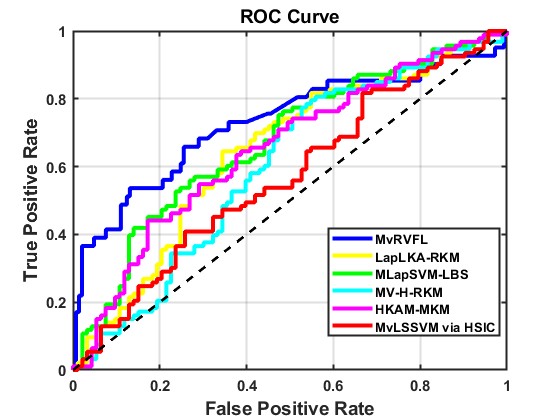
(b) NMBAC & PSSM-DWT

(c) MCD & PsePSSM

Figure 6: ROC curves of the proposed MvRVFL model along with DNA binding protein prediction models.

6.2.2 Comparison of the proposed model with the existing DNA binding prediction models

We compare our proposed MvRVFL model with existing DNA binding protein prediction models, including MvLSSVM via HSIC (Zhao et al., 2022b), HKAM-MKM (Zhao et al., 2022a), MV-H-RKM (Guan et al., 2022), MLapSVM-LBS (Sun et al., 2022), and LapLKA-RKM (Qian et al., 2023). Table 4 demonstrates that all five features (MCD, NMBAC, PSSM-DWT, PsePSSM, and PSSM-AB) are beneficial for predicting DBPs using MvRVFL. Among these, MCD_vs_PsePSSM achieves the best result (Acc. = $80.11\%$). This suggests that PsePSSM is a crucial feature for predicting DBPs. From Table 4, the average accuracy of the proposed MvRVFL-1 and MvRVFL-2 models are $76.32\%$ and $74\%$, respectively. The average Acc. of the proposed models surpasses that of the baseline models. The proposed MvRVFL-1 and MvRVFL-2 exhibit exceptional generalization performance, marked by consistently higher Acc., indicating a high level of confidence in their learning process. It is found that the MvRVFL model is comparable to the baseline models in most cases. By incorporating the coupling term, MvRVFL can integrate information from both views. This approach allows for a larger error variable in one view if it is compensated by the other view by minimizing the product of the error variables. The Seny., Spey., and Pren. indicate that the proposed MvRVFL-1 model performs competitively compared to the baseline models. The MvRVFL-1 model demonstrates strong performance in all these areas, showing its robustness and reliability in comparison with existing models.

Figure 6 illustrates the ROC curve, showcasing the superior performance of the proposed MvRVFL model compared to baseline models on the DNA-binding proteins datasets. The ROC curve provides a comprehensive evaluation of the model’s diagnostic capabilities by plotting the true positive rate (Seny.) against the false positive rate (1 - Spey.) across various threshold settings. The area under the ROC curve (AUC) for the proposed MvRVFL model is significantly higher, indicating a better balance between Seny. and Spey..

A higher AUC demonstrates that the MvRVFL model is more effective at distinguishing between positive and negative instances, leading to more accurate predictions. This increased AUC signifies the model’s enhanced ability to correctly identify true positives while minimizing false negatives, thereby ensuring more reliable detection.

The superior performance of the MvRVFL model can be attributed to the inclusion of crucial features, particularly PsePSSM. PsePSSM captures essential evolutionary information from the protein sequences, providing a more comprehensive representation that significantly contributes to the model’s predictive accuracy. By leveraging PsePSSM, the model benefits from detailed sequence order information, which enhances its ability to correctly classify DBPs.

These results underscore the robustness and effectiveness of the MvRVFL model in classification tasks, surpassing the performance of baseline models. The importance of PsePSSM as a feature is evident, as it plays a pivotal role in improving the model’s overall accuracy and reliability in identifying true positives and reducing false negatives.

Figure 7: Ablation study of the coupling term for MvRVFL: The x-axis represents the datasets indexed in Table 4, and the y-axis represents the Acc. ($\%$).

6.2.3 Ablation study

To validate our claim that the coupling term acts as a bridge among multiple views, enhancing the coordination between different features and thereby improving the training efficiency of the proposed MvRVFL model, we conducted an ablation study. In this study, we set the coupling term to zero ($\rho=0$) in the optimization (5) to assess its true impact. The results, depicted in Fig. 7, demonstrate that the MvRVFL model consistently outperforms the model without coupling term across most datasets, confirming the effectiveness of the coupling term.

This outcome verifies the critical role of the coupling term $\rho$ in the model’s architecture. The coupling term allows the MvRVFL model to effectively integrate information from both the image views and the caption view. By minimizing the product of the error variables from both views, the model can tolerate a larger error in one view if it is offset by a smaller error in the other view. This balancing mechanism enhances the overall reliability and robustness of the model, leading to more accurate and dependable results.

The ablation study clearly demonstrates that incorporating the coupling term enables the MvRVFL model to better manage the complementary information from different views, resulting in improved performance and more reliable predictions.

Table 4: Performance comparison of the proposed MvRVFL-1 and MvRVFL-2 along with DNA binding protein prediction models.

Dataset	Dataset	MvLSSVM via HSIC	HKAM-MKM	MV-H-RKM	MLapSVM-LBS	LapLKA-RKM	MvRVFL-1†	MvRVFL-2†
index	name	(Zhao et al., 2022b)	(Zhao et al., 2022a)	(Guan et al., 2022)	(Sun et al., 2022)	(Qian et al., 2023)
		(Acc., Seny.)	(Acc., Seny.)	(Acc., Seny.)	(Acc., Seny.)	(Acc., Seny.)	(Acc., Seny.)	(Acc., Seny.)
		(Spey., Pren.)	(Spey., Pren.)	(Spey., Pren.)	(Spey., Pren.)	(Spey., Pren.)	(Spey., Pren.)	(Spey., Pren.)
1.	MCD_vs_NMBAC	$(74.47,77.78)$	$(72.96,73.04)$	$(65.7,74.06)$	$(61.7,81.03)$	$(68.85,86.54)$	$(75.27,89.25)$	$(68.92,79.89)$
		$(83.45,87.93)$	$(81.08,78.46)$	$(82.17,82.93)$	$(90.78,82.51)$	$(82.41,80.77)$	$(77.64,89.25)$	$(97.85,75.45)$
2.	MCD_vs_PSSM-AB	$(74.58,82.35)$	$(71.72,71.79)$	$(69.46,72.82)$	$(74.82,73.85)$	$(63.64,77.89)$	$(75.81,74.19)$	$(74.04,80.65)$
		$(61.33,76.27)$	$(60.67,70.81)$	$(58.59,77.67)$	$(57.48,73.25)$	$(59.8,72.81)$	$(60.53,74.19)$	$(63.44,68.81)$
3.	MCD_vs_PSSM-DWT	$(66.57,89.44)$	$(67.74,86.92)$	$(60,84.58)$	$(65.69,89.34)$	$(66.21,81.84)$	$(69.42,91.4)$	$(66.92,83.23)$
		$(72.59,89.09)$	$(70.15,80.33)$	$(75.67,84.48)$	$(70.18,85.23)$	$(79.71,71.43)$	$(60.28,91.4)$	$(94.62,87.5)$
4.	MCD_vs_PsePSSM	$(66.99,72.14)$	$(73.11,74.8)$	$(79.46,74.63)$	$(76.47,76.56)$	$(78.66,78.41)$	$(80.11,78.49)$	$(76.45,75.48)$
		$(70.88,76.86)$	$(71.04,77.58)$	$(69.55,72.3)$	$(74.78,71.78)$	$(76.79,78.72)$	$(77.03,78.49)$	$(77.42,61.11)$
5.	NMBAC_PSSM-DWT	$(75.34,73.61)$	$(76.34,78.52)$	$(67.03,74.89)$	$(72.88,80)$	$(74.13,79.59)$	$(76.88,81.06)$	$(76.98,80)$
		$(81.99,70.36)$	$(80.53,54.22)$	$(87.16,64.75)$	$(73.33,57.14)$	$(84.67,72.24)$	$(67.42,64.52)$	$(100,75.82)$
6.	NMBAC_vs_PSSM-AB	$(76.47,80.96)$	$(71.39,78.23)$	$(77.78,74.7)$	$(76.57,73.65)$	$(73.75,75.38)$	$(78.49,81.98)$	$(75.85,78.25)$
		$(82.03,75.44)$	$(75.97,70.49)$	$(73.95,72.88)$	$(88.71,73.41)$	$(78.46,65.29)$	$(66.32,67.74)$	$(100,75.23)$
7.	NMBAC_vs_PsePSSM	$(74.57,74.19)$	$(76.32,82.27)$	$(77.27,79.35)$	$(76.99,80.33)$	$(79.35,81.6)$	$(80.8,85.05)$	$(80.54,76.13)$
		$(70.33,75.16)$	$(85.04,80.82)$	$(83.96,77.41)$	$(75.15,74.97)$	$(80.81,71.38)$	$(61.8,79.14)$	$(84.95,81.72)$
8.	PSSM-AB_vs_PSSM-DWT	$(77.53,74.55)$	$(90.86,67.77)$	$(91.3,67.83)$	$(55.34,76.12)$	$(62.12,76.62)$	$(76.34,79.82)$	$(72.89,77.2)$
		$(72.79,73.49)$	$(81.29,78.43)$	$(80.05,70.18)$	$(78.85,71.58)$	$(80.33,79.82)$	$(71.15,79.57)$	$(82.8,80)$
9.	PsePSSM_vs_PSSM-AB	$(74.4,84.29)$	$(74.37,76.6)$	$(73.48,79.44)$	$(76.47,82.59)$	$(74.74,80.97)$	$(75.65,83.49)$	$(74.54,80.43)$
		$(79.51,78.97)$	$(72.13,76.67)$	$(71.65,77.8)$	$(77.93,78.35)$	$(74.58,65.22)$	$(67.29,77.42)$	$(80.65,71.35)$
10.	PsePSSM_vs_PSSM-DWT	$(75.82,76.21)$	$(75.84,72.26)$	$(73.04,75.65)$	$(72.31,74.78)$	$(71.93,82.47)$	$(74.41,86.38)$	$(72.91,84.73)$
		$(88.98,69.68)$	$(82.26,75.51)$	$(80.16,76.67)$	$(76.27,82.8)$	$(84.22,81.02)$	$(92.36,85.45)$	$(87.1,65.71)$
	Average Acc.	$73.67$	$75.07$	$73.45$	$70.92$	$71.34$	76.32	$74$
Seny., Spey., and Pren. denote the Sensitivity, Specificity, and Precision, respectively.
† represents the proposed models.

6.2.4 Sensitivity of $C_{1}$ and $\rho$ combinations

In this subsection, we evaluate the impact of the regularization parameters $\mathcal{C}_{1}$ and $\rho$ of MvRVFL. In Fig. 8, the values of $\mathcal{C}_{1}$ and $\rho$ are varied from $10^{-5}$ to $10^{5}$, keeping the other parameters is fixed at their optimal values and the corresponding Acc. values are recorded. The performance of MvRVFL is depicted under different parameter settings $\mathcal{C}_{1}$ and $\rho$. The parameter $\rho$ serves as a coupling term designed to minimize the product of error variables between Vw-$A$ and Vw-$B$. When $\mathcal{C}_{1}$ lies between $10^{-1}$ and $10^{5}$ with the same value of $\rho$, there is a corresponding improvement observed in the Acc. values. These findings suggest that when evaluating parameters $\mathcal{C}_{1}$ and $\rho$, the model’s performance is primarily influenced by $\mathcal{C}_{1}$ rather than $\rho$. Therefore, meticulous selection of hyperparameters for the proposed MvRVFL model is essential to achieve optimal generalization performance.

6.2.5 Influence of the number of hidden nodes $h_{1}$

To fully comprehend the robustness of the proposed MvRVFL model, it’s crucial to analyze their sensitivity to the number of hidden nodes $h_{l}$. The influence of the hyperparameter $h_{l}$ is depicted in Fig. 9. Fig. 9a and 9c show that the performance peaks at $h_{l}=23$ and then gradually declines as $h_{l}$ increases further. Therefore, to achieve the best performance from the MvRVFL, we recommend using $h_{l}=23$. The performance peaks at $h_{l}=23$ and $h_{l}=83$ and then gradually declines as $h_{l}$ increases further depicted in Fig. 9d. From Fig. 9b, the performance consistently improves with an increase in the number of hidden nodes until reaching a plateau. Optimal performance is typically achieved with higher values of $h_{l}$. We recommend fine-tuning the hyperparameters to attain the best performance from the proposed models for specific tasks.

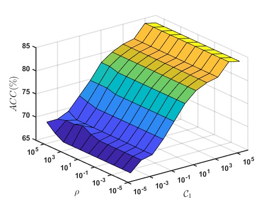
(a) MCD & NMBAC

(b) MCD & PSSM-DWT

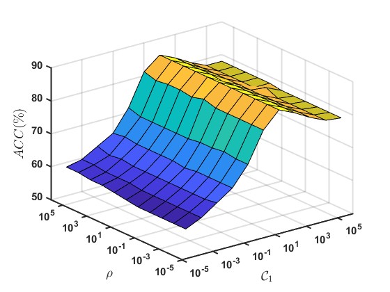
(c) NMBAC & PSSM-DWT

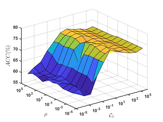
(d) NMBAC & PSSM-AB

Figure 8: Effect of parameters $\mathcal{C}_{1}$ and $\rho$ on the performance of the proposed MvRVFL model.

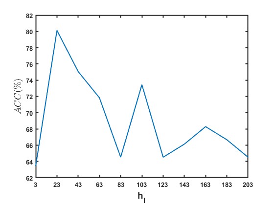
(a) MCD & PsePSSM

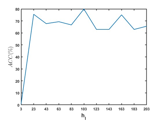
(b) MCD & PSSM-AB

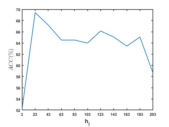
(c) MCD & PSSM-DWT

(d) PsePSSM & PSSM-DWT

Figure 9: Effect of parameter $h_{l}$ on the performance of the proposed MvRVFL model.

6.3 Evaluation on UCI and KEEL Datasets

In this section, we present a comprehensive analysis, including a comparison of the proposed MvRVFL model with baseline models across $27$ UCI (Dua & Graff, 2017) and KEEL (Derrac et al., 2015) benchmark datasets. Considering that the UCI and KEEL datasets do not inherently possess multiview characteristics, we use the $95\%$ principal component to reduce the feature from the original data and it is given as Vw-$B$, and we refer to the original data as Vw-$A$ (Wang et al., 2023). The performance of the proposed MvRVFL model along with the baseline models is evaluated using Acc. metrics along with the corresponding optimal hyperparameters., as depicted in Table 7 of Appendix. The average Acc. for the proposed MvRVFL-1 and MvRVFL-2 models along with the baseline SVM2K, MvTSVM, ELM-Vw-$A$, ELM-Vw-$B$, RVFL-Vw-$A$, RVFL-Vw-$B$, and MVLDM models are $85.15\%$, $83.18\%$, $76.65\%$, $67.24\%$, $82.66\%$, $81.7\%$, $83.14\%$, $81.26\%$, and $79.9\%$, respectively. In terms of average Acc., the proposed MvRVFL-1 achieved the top position, while the proposed MvRVFL-2 ranked second. This demonstrates that the proposed MvRVFL-1 and MvRVFL-2 models exhibit a significant level of confidence in their predictive capabilities. Average Acc. can be misleading because it might obscure a model’s superior performance on one dataset by offsetting its inferior performance on another. To address the limitations of average Acc. and ascertain the significance of the results, we employed a suite of statistical tests recommended by (Demšar, 2006). These tests are tailor-made for comparing classifiers across multiple datasets, especially when the conditions required for parametric tests are not satisfied. We utilized the following tests: ranking test, Friedman test, Nemenyi post hoc test, and win-tie loss sign test. By integrating statistical tests, our objective is to comprehensively evaluate the performance of the models, facilitating us to draw broad and unbiased conclusions regarding their effectiveness. In the ranking scheme, each model receives a rank according to its performance on individual datasets, allowing for an evaluation of its overall performance. Higher ranks are attributed to the worst-performing models, while lower ranks are assigned to the best-performing models. By employing this methodology, we consider the potential compensatory effect wherein superior performance on one dataset offsets inferior performance on others. For evaluation of $q$ models across $N$ datasets, the rank of the $j^{th}$ model on the $i^{th}$ dataset can be denoted as $\mathfrak{R}_{j}^{i}$. Then the $j^{th}$ model’s average rank is given by $\mathfrak{R}_{j}=\frac{1}{N}\sum_{i=1}^{N}\mathfrak{R}_{j}^{i}.$ The rank of the proposed MvRVFL-1 and MvRVFL-2 models along with the baseline SVM2K, MvTSVM, ELM-Vw-$A$, ELM-Vw-$B$, RVFL-Vw-$A$, RVFL-Vw-$B$, and MVLDM models are $2.04$, $3.20$, $6.35$, $8.65$, $4.70$, $5.26$, $4.22$, $5.09$, and $5.48$, respectively. Table 5 displays the average ranks of the models. The MvRVFL-1 model attained an average rank of $2.04$, which is the lowest among all the models. While the proposed MvRVFL-2 attained the second position with an average rank of $3.20$. Given that a lower rank signifies a better-performing model, the proposed MvRVFL-1 and MvRVFL-2 models emerged as the top-performing model. The Friedman test (Friedman, 1937) compares whether significant differences exist among the models by comparing their average ranks. The Friedman test, a nonparametric statistical analysis, is utilized to compare the effectiveness of multiple models across diverse datasets. Under the null hypothesis, the models’ average rank is equal, implying that they give equal performance. The Friedman test adheres to the chi-squared distribution ($\chi_{F}^{2}$) with $(q-1)$ degree of freedom (d.o.f) and its calculation involves: $\chi^{2}_{F}=\frac{12N}{q(q+1)}\left[\sum_{j}\mathfrak{R}_{j}^{2}-\frac{q(q+1)^{2}}{4}\right].$ The $F_{F}$ statistic is calculated as: $F_{F}=\frac{(N-1)\chi_{F}^{2}}{N(q-1)-\chi_{F}^{2}}$, where $F$- distribution has $(q-1)$ and $(N-1)\times(q-1)$ degrees of freedom. For $N=27$ and $q=9$, we obtained $\chi_{F}^{2}=100.983$ and $F_{F}=22.8276$. From the $F$-distribution table at a significance level of $5\%$, the value of $F_{F}(8,208)=1.9831$. As $F_{F}>1.9831$, the null hypothesis is rejected. Hence, notable discrepancies are evident among the models. Consequently, we proceed to employ the Nemenyi post hoc test (Demšar, 2006) to assess the pairwise differences between the models. C.D. = $q_{\alpha}\times\sqrt{\frac{q(q+1)}{6N}}$ is the critical difference (C.D.). Here, $q_{\alpha}$ denotes the critical value obtained from the distribution table for the two-tailed Nemenyi test. Referring to the statistical F-distribution table, where $q_{\alpha}=3.102$ at a $5\%$ significance level, the C.D. is computed as $2.3120$. The average rank differences between the proposed MvRVFL-1 and MvRVFL-2 models with the baseline SVM2K, MvTSVM, ELM-Vw-$A$, ELM-Vw-$B$, RVFL-Vw-$A$, RVFL-Vw-$B$, and MVLDM models are $(4.31,3.15)$, $(6.61,5.45)$, $(2.66,1.50)$, $(3.22,2.06)$, $(2.18,1.02)$, $(3.05,1.89)$, and $(3.44,2.28)$. The Nemenyi post hoc test validates that the proposed MvRVFL-1 model exhibits statistically significant superiority compared to SVM2K, MvTSVM, ELM-Vw-$A$, ELM-Vw-$B$, RVFL-Vw-$B$, and MVLDM. The proposed MvRVFL-2 models observed a statistically significant compared to the SVM2K and MvTSVM models.

Table 5: Average Acc. and average rank of the proposed MvRVFL-1 and MvRVFL-2 along with the baseline models based on classification Acc. for UCI, KEEL, AwA, and Corel5K datasets.

	Dataset	SVM2K	MvTSVM	ELM-Vw-$A$	ELM-Vw-$B$	RVFL-Vw-$A$	RVFL-Vw-$B$	MVLDM	MvRVFL-1†	MvRVFL-2†
		(Farquhar et al., 2005)	(Xie & Sun, 2015)	(Huang et al., 2006)	(Huang et al., 2006)	(Pao et al., 1994)	(Pao et al., 1994)	(Hu et al., 2024)
UCI and KEEL	Average Acc.	$76.65$	$67.24$	$82.66$	$80.95$	$83.14$	$81.26$	$79.9$	85.15	$83.18$
	Average Rank	$6.35$	$8.65$	$4.70$	$5.26$	$4.22$	$5.09$	$5.48$	$2.04$	$3.20$
AwA	Average Acc.	$77.46$	$64.31$	$71.74$	$75.99$	$72.87$	$77.46$	$73.33$	82.50	$77.97$
	Average Rank	$4.08$	$7.71$	$6.82$	$4.9$	$6.06$	$4.26$	$5.74$	$1.63$	$3.8$
Corel5k	Average Acc.	$74.87$	$49.93$	$74.98$	$74.83$	$76.33$	$75.43$	$69.87$	78.01	$75.63$
	Average Rank	$4.75$	$8.93$	$4.58$	$4.56$	$3.85$	$4.60$	$6.33$	$3.03$	$4.37$
† represents the proposed models.

Table 6: Pairwise win-tie-loss test of proposed MvRVFL-1 and MvRVFL-2 models along with baseline models on UCI and KEEL datasets.

	SVM2K	MvTSVM	ELM-Vw-$A$	ELM-Vw-$B$	RVFL-Vw-$A$	RVFL-Vw-$B$	MVLDM	MvRVFL-1†
	(Farquhar et al., 2005)	(Xie & Sun, 2015)	(Huang et al., 2006)	(Huang et al., 2006)	(Pao et al., 1994)	(Pao et al., 1994)	(Hu et al., 2024)
MvTSVM (Xie & Sun, 2015)	[$2,2,23$]
ELM-Vw-$A$ (Huang et al., 2006)	[$18,1,8$]	[$27,0,0$]
ELM-Vw-$B$ (Huang et al., 2006)	[$18,2,7$]	[$26,0,1$]	[$9,4,14$]
RVFL-Vw-$A$ (Pao et al., 1994)	[$21,1,5$]	[$27,0,0$]	[$11,10,6$]	[$15,4,8$]
RVFL-Vw-$B$ (Pao et al., 1994)	[$18,1,8$]	[$25,1,1$]	[$9,5,13$]	[$11,9,7$]	[$7,7,13$]
MVLDM (Hu et al., 2024)	[$16,1,10$]	[$24,0,3$]	[$11,0,16$]	[$12,0,15$]	[$9,0,18$]	[$13,0,14$]
MvRVFL-1†	[$24,2,1$]	[$27,0,0$]	[$22,1,4$]	[$24,2,1$]	[$20,4,3$]	[$24,2,1$]	[$24,0,3$]
MvRVFL-2†	[$22,1,4$]	[$25,2,0$]	[$19,1,7$]	[$20,1,6$]	[$18,2,7$]	[$18,2,7$]	[$20,1,6$]	[$8,3,16$]
† represents the proposed models.

Furthermore, to evaluate the models, we employ the pairwise win-tie-loss sign test. This test assumes, under the null hypothesis, that two models perform equivalently and are expected to win in $N/2$ datasets, where $N$ represents the dataset count. If the model wins on approximately $\frac{N}{2}+1.96\frac{\sqrt{N}}{2}$ datasets, then the model is deemed significantly better. If the number of ties between the two models is even, these ties are distributed equally between them. However, if the number of ties is odd, one tie is excluded, and the remaining ties are distributed among the classifiers. In this case, with $N=27$, if one of the models records at least $18.59$ wins, it indicates a significant difference between the models. Table 6 presents a comparative analysis of the proposed MvRVFL-1 and MvRVFL-2 models alongside the baseline models. In Table 6, the entry $[x,y,z]$ denotes the number of times the model listed in the row wins $x$, ties $y$, and loses $z$ when compared to the model listed in the corresponding column. The proposed MvRVFL-2 model attains a statistically significant difference from the baseline models, except RVFL-Vw-$A$ and RVFL-Vw-$B$. The winning percentage of MvRVFL-2 continues to demonstrate its effectiveness over the RVFL-Vw-$A$ and RVFL-Vw-$B$ models. The evidence demonstrates that the proposed MvRVFL-1 and MvRVFL-2 models exhibit significant superiority when compared to the baseline models.

6.4 Evaluation on AwA and Corel5k Dataset

In this subsection, we perform an in-depth analysis, comparing the proposed MvRVFL model with baseline models using the AwA dataset, which comprises $30,475$ images of $50$ animal classes, each represented by six preextracted features for every image. For our evaluation, we utilize ten test classes: Persian cat, leopard, raccoon, chimpanzee, humpback whale, giant panda, pig, hippopotamus, seal, and rat, totaling $6180$ images. The $2000$-dimensional $L_{1}$ normalized speeded-up robust features (SURF) are denoted as Vw-$A$, while the $252$-dimensional histogram of oriented gradient features descriptors is represented as Vw-$B$. For each combination of class pairs, we employ the one-against-one strategy to train $45$ binary classifiers. The Corel5k dataset consists of $50$ categories, each comprising $100$ images representing various semantic topics, such as bus, dinosaur, beach, and more. The $512$-dimensional GIST features are denoted as Vw-$A$, while the $100$-dimensional DenseHue features are denoted as Vw-$B$. In the experiments, we utilize a one-versus-rest scenario for each category individually, training $50$ binary classifiers accordingly. We randomly choose $100$ images from the other classes and include $100$ images from the target class in each binary dataset.

The performance evaluation of the proposed MvRVFL models, alongside the baseline models, is conducted using Acc. metrics and the corresponding optimal hyperparameters, which are reported in Tables 8 and 9 on AwA and Corel5K datasets of the Appendix and the average Acc. is reported in Table 5. We can infer the following conclusions: Firstly, MvRVFL models attain the highest average Acc., the lowest average rank, and the most wins, indicating their superior performance. Secondly, although the MvRVFL models performance is slightly inferior in some instances, it remains competitive, with results closely approaching the best outcomes. Thirdly, across most datasets, MvRVFL demonstrates higher accuracies compared to SVM-2K. This highlights the capability of MvRVFL models to effectively utilize two views by adhering to the coupling term that minimizes the product of the error variables for both views, leading to enhanced classification performance. In the Appendix, we perform several sensitivity analyses on different aspects of the proposed models. This involves examining how the parameters $\mathcal{C}_{1}$ and $\mathcal{C}_{2}$ affect the proposed models in subsection A.2.1. We conduct experiments with varying numbers of training samples on the AwA dataset, as discussed in subsection A.2.2. Finally, we conduct the sensitivity of $\theta$ and $\rho$ discussed in subsection A.3.1.

7 Conclusion and Future Work

In this paper, we proposed a novel multiview random vector functional link (MvRVFLs) network for the prediction of DBP. The proposed MvRVFL models not only extract rich feature representations through the hidden layers of multiple views but also serve as a weighting network. It allocates weights to features from all hidden layers, including the original features acquired via direct links. The coupling of different views in the MvRVFL models is achieved by incorporating the coupling term in the primal formulation of the model. The outstanding performance of MvRVFL (compared to the baseline models) in DBP is primarily attributed to the fusion of features extracted from protein sequences, including PsePSSM, PSSM-DWT, NMBAC, MCD, and PSSM-AB. Furthermore, we conducted experiments on UCI, KEEL, AwA, and Corel5K datasets. The experimental results, along with the statistical analyses, indicate that the proposed MvRVFL models beat the baseline models in terms of generalization performance. In future research, we aim to extend the proposed model to tackle class-imbalanced problems with multiple views (more than two views). Also, we intend to enhance the feature representation method and devise predictive models that synergistically integrate diverse features more effectively.

Appendix A Appendix

Here, we begin with a discussion on the generalization capability of the proposed MvRVFL model, followed by sensitivity analyses of the key hyperparameters involved. Lastly, we present detailed tables reporting the accuracy and the best hyperparameters.

A.1 Generalization Capability Analysis

Here, we discuss the generalization error bound for the MvRVFL model. In this analysis, we used the label $y_{i}\in\{-1,+1\}$ instead of employing one-hot encoding. The optimization problem of the MvRVFL model is reformulated as follows:

$$\underset{\beta_{1},\beta_{2}}{\min}\hskip 5.69046pt \frac{1}{2}\|\beta_{1}\|^{2}+\frac{\theta}{2}\|\beta_{2}\|^{2}+\frac{\mathcal{C}_{1}}{2}\sum_{i=1}^{n}\xi_{1_{i}}^{T}\xi_{1_{i}}+\frac{\mathcal{C}_{2}}{2}\sum_{i=1}^{n}\xi_{2_{i}}^{T}\xi_{2_{i}}+\rho\sum_{i=1}^{n}\xi_{1_{i}}^{t}\xi_{2_{i}}$$

s.t. $$Z_{1}^{(x_{i})}\beta_{1}-y_{i}=\xi_{1_{i}},$$

$$Z_{2}^{(x_{i})}\beta_{2}-y_{i}=\xi_{2_{i}},\hskip 5.69046pti=1,2,\ldots,n.$$ (37)

If we multiply by $y_{i}$ on both sides of the constraints of Eq. (A.1), it results in

$$y_{i}Z_{1}^{(x_{i})}\beta_{1}-1=y_{i}\xi_{1_{i}},$$ (38)

$$y_{i}Z_{2}^{(x_{i})}\beta_{2}-1=y_{i}\xi_{2_{i}},\hskip 5.69046pti=1,2,\ldots,n,$$ (39)

Eqs. (38) and (39) are used in the theorem 2.

To start, we define the Rademacher complexity (Bartlett & Mendelson, 2002) as follows:

Definition 1.

For the set of samples, $S=\{x_{1},\ldots,x_{n}\}$, consisting of $n$ independent samples from the distribution $\mathcal{D}$ and the function set $\mathscr{G}$ on $S$, we define the empirical Rademacher complexity on $\mathscr{G}$ as:

$$\hat{R}_{n}({\mathscr{G}}) =\mathbb{E}_{\sigma}\left[\underset{g\in\mathscr{G}}{\sup}|\frac{2}{n}\sum_{i=1}^{n}\sigma_{i}g(x_{i})|:x_{1},x_{2},\ldots,x_{n}\right],$$ (40)

where $\sigma=(\sigma_{1},\ldots,\sigma_{n})$ are independently uniform valued $\{+1,-1\}$ (Rademacher) random variables. The Rademacher complexity of $\mathscr{G}$ is given by:

$$R_{n}(\mathscr{G}) =\hat{\mathbb{E}}_{S}[\hat{R}_{n}(\mathscr{G})]=\hat{\mathbb{E}}_{S\sigma}\left[\underset{g\in\mathscr{G}}{\sup}|\frac{2}{n}\sum_{i=1}^{n}\sigma_{i}g(x_{i})|\right].$$ (41)

Lemma 1.

Choose $\theta$ from the interval $(0,1)$ and consider $\mathscr{G}$ as a class of functions mapping from an input space $S$ to $[0,1]$. Suppose $\{x_{i}\}_{i=1}^{n}$ are drawn independently from a probability distribution $\mathcal{D}$. Then, with a probability of at least $1-\theta$ over random samples of size $n$, every $g\in\mathscr{G}$ satisfies:

$$\mathbb{E}_{\mathcal{D}}[g(x)]\leq\hat{\mathbb{E}}_{\mathcal{D}}[g(x)]+\hat{R}_{n}(\mathscr{G})+3\sqrt{\frac{\ln(2/\theta)}{2n}}.$$ (42)

Lemma 2.

Let $S=\{(x_{i},y_{i})\}_{i=1}^{n}$ be a sample set and $Z^{(x)}$ be the enhanced feature matrix. For the function class $\mathscr{G}_{B}=\{g|g:x\rightarrow\lvert Z^{(x)}\beta\rvert,\|\beta\|\leq B\}$ then, the empirical Rademacher complexity of $\mathscr{G}_{B}$ satisfies:

$$\hat{R}_{n}(\mathscr{G}_{B})=\frac{2B}{n}\sqrt{\sum_{i=1}^{n}Z^{(x_{i})^{T}}Z^{(x_{i})}}$$ (43)

Lemma 3.

Consider $\mathscr{A}$ as a Lipschitz function with a Lipschitz constant $\mathcal{L}$, mapping the real numbers to the real numbers, satisfying $\mathscr{A}(0)=0$. The Rademacher complexity of the class $\mathscr{A}\circ\mathscr{G}$ is:

$$\hat{R}_{n}(\mathscr{A}\circ\mathscr{G})\leq 2\mathcal{L}\hat{R}_{n}(\mathscr{G}).$$ (44)

We define the difference between the final predictors of the two views as $g_{m}(x)=\lvert Z_{1}^{(x)}\beta_{1}-Z_{2}^{(x)}\beta_{2}\rvert$. Thus, the true expectation bound of $g_{m}(x)$ can be derived using the following theorem.

Theorem 1.

Given $N\in\mathbb{R}^{+}$, $\theta\in(0,1)$, and a training set $T=\{(x_{i},y_{i})\}_{i=1}^{n}$ drawn independently and identically from probability distribution $\mathcal{D}$, where $y_{i}\in\{-1,+1\}$ and $x_{i}=(x_{i}^{A};x_{i}^{B})$. Define the function class $\mathscr{G}_{N}=\{g|g:x\rightarrow\lvert Z^{(x)}\beta\rvert,\|\beta\|\leq N\}$ and $\hat{\mathscr{G}}_{N}=\{\hat{g}|\hat{g}:x\rightarrow Z^{(x)}\beta,\|\beta\|\leq N\}$, where $\beta=(\beta_{1};\beta_{2})$, $Z^{(x)}=\left(Z_{1}^{(x)};-Z_{2}^{(x)}\right)=\left([x^{A}\hskip 5.69046pt\phi(x^{A}W^{A}+b^{A})];-[x^{B}\hskip 5.69046pt\phi(x^{B}W^{B}+b^{B})]\right)$ and $g_{m}(x)=\lvert Z_{1}^{(x)}\beta_{1}-Z_{2}^{(x)}\beta_{2}\rvert=\lvert Z^{(x)}\beta\rvert\in\mathscr{G}_{N}$. Then, with a probability of at least $1-\theta$ over $T$, every $g_{m}(x)\in\mathscr{G}_{N}$ satisfies

$$\mathbb{E}_{\mathcal{D}}[g_{m}(x)]\leq 2N+3N\mathcal{K}_{m}\sqrt{\frac{\ln(2/\theta)}{2n}}+\frac{4N}{n}\sqrt{\sum_{i=1}^{n}(\|Z_{1}^{(x_{i})}\|^{2}+\|Z_{2}^{(x_{i})}\|^{2})},$$ (45)

where

$$\mathcal{K}_{m}=\underset{x_{i}\in\sup(\mathcal{D})}{\max}\sqrt{\|Z_{1}^{(x_{i})}\|^{2}+\|Z_{2}^{(x_{i})}\|^{2}}.$$ (46)

Proof.

Let’s consider a loss function $\Omega:\mathbb{R}\rightarrow[0,1]$ defined as:

$$\Omega=\left\{\begin{array}[]{lll}{-\frac{x}{N\mathcal{K}_{m}}},&\text{if}\leavevmode\nobreak\ \leavevmode\nobreak\ -N\mathcal{K}_{m}\leq x<0,\vspace{3mm}\\ {\frac{x}{N\mathcal{K}_{m}}},&\text{if}\leavevmode\nobreak\ \leavevmode\nobreak\ 0\leq x\leq N\mathcal{K}_{m},\\ {1},&\text{otherwise}.\end{array}\right.$$ (50)

For an independently drawn sample $(x_{i},y_{i})$ from the probability distribution $\mathcal{D}$, combining $\|\beta\|\leq N$ with Eq. (46), we obtain:

$$g_{m}(x_{i}) =\lvert Z^{(x_{i})}\beta\rvert\leq N\|Z^{(x_{i})}\|$$

$$=N\sqrt{\|Z_{1}^{(x_{i})}\|^{2}+\|Z_{2}^{(x_{i})}\|^{2}}\leq N\mathcal{K}_{m}.$$ (51)

In that case, $g_{m}(x)$ ranges from $0$ to $N\mathcal{K}_{m}$, while $\hat{g}_{m}(x)$ ranges from $-N\mathcal{K}_{m}$ to $N\mathcal{K}_{m}$. According to Lemma 1 and with $\Omega(\hat{g}_{m}(x))$ ranging from $0$ to $1$, the following inequality holds with a probability of at least $1-\theta$ over $T$:

$$\mathbb{E}_{\mathcal{D}}[\Omega(\hat{g}_{m}(x))]\leq\hat{\mathbb{E}}_{T}[\Omega(\hat{g}_{m}(x))]+\hat{R}_{n}(\Omega\circ\hat{\mathscr{G}}_{N})+3\sqrt{\frac{\ln(2/\theta)}{2n}}.$$ (52)

Given that $\Omega(x)$ is a Lipschitz function with a constant of $\frac{1}{N\mathcal{K}_{m}}$, passes through the origin, and is uniformly bounded, we can assert the following inequality based on Lemmas 2 and 3:

$$\hat{R}_{n}(\Omega\circ\hat{\mathscr{G}}_{N}) \leq\frac{4}{n\mathcal{K}_{m}}\sqrt{\sum_{i=1}^{n}\|Z^{(x_{i})}\|^{2}}$$

$$=\frac{4}{n\mathcal{K}_{m}}\sqrt{\sum_{i=1}^{n}(\|Z_{1}^{(x_{i})}\|^{2}+\|Z_{2}^{(x_{i})}\|^{2})}.$$ (53)

Hence,

$$\mathbb{E}_{\mathcal{D}}[\Omega(\hat{g}_{m}(x))]\leq\hat{\mathbb{E}}_{T}[\Omega(\hat{g}_{m}(x))]+3\sqrt{\frac{\ln(2/\theta)}{2n}}+\frac{4}{n\mathcal{K}_{m}}\sqrt{\sum_{i=1}^{n}(\|Z_{1}^{(x_{i})}\|^{2}+\|Z_{2}^{(x_{i})}\|^{2})}.$$ (54)

Since $g_{m}(x_{i})=N\mathcal{K}_{m}\Omega(\hat{g}_{m}(x))$, we have

$$\mathbb{E}_{\mathcal{D}}[g_{m}(x)] =N\mathcal{K}_{m}\mathbb{E}_{\mathcal{D}}[\Omega(\hat{g}_{m})]$$

$$\leq\hat{\mathbb{E}}_{T}[g_{m}(x)]+3N\mathcal{K}_{m}\sqrt{\frac{\ln{(2/\theta)}}{2n}}+\frac{4N}{n}\sqrt{\sum_{i=1}^{n}(\|Z_{1}^{(x_{i})}\|^{2}+\|Z_{2}^{(x_{i})}\|^{2})}.$$ (55)

Also,

$$\lvert Z^{(x_{1})}\beta\rvert\leq N\lvert Z^{(x_{i})}\rvert=N\lvert Z_{1}^{(x_{i})}-Z_{2}^{(x_{i})}\rvert\leq N(\lvert Z_{1}^{(x_{i})}\rvert+\lvert Z_{2}^{(x_{i})}\rvert)\leq 2N$$ (56)

We can obtain,

$$\hat{\mathbb{E}}_{T}[g_{m}(x)]=\hat{\mathbb{E}}_{T}[Z^{(x)}\beta]\leq 2N.$$ (57)

From Eqs. (A.1) and (57), we can conclude the theorem. ∎

Consistency plays a crucial role in MVL, aiming to reduce the discrepancy in predictions across different perspectives or views. A lower consistency error typically results in improved generalization performance. We represent $g_{m}(x)$ as the consistency error function between the two views. Next, by applying the empirical Rademacher complexity of the function classes $\hat{\mathscr{G}}_{m}$ along with the empirical expectation of $g_{m}$, we obtain a margin-based estimate for the consistency error expectation. MvRVFL demonstrates a tight consensus error bound as $n$ becomes sufficiently large. As the consistency error during training decreases, the generalization error likewise decreases. This theoretical assurance underscores MvRVFL’s robust generalization performance concerning consistency.

Next, we examine the generalization error bound. According to (32), we use the weighted combination of predictions from the two views to define the prediction function for MvRVFL. Therefore, the generalization error bound for MvRVFL can be determined using the following theorem.

Theorem 2.

Given $N\in\mathbb{R}^{+}$, $\theta\in(0,1)$, and a training set $T=\{(x_{i},y_{i})\}_{i=1}^{n}$ drawn independently and identically from probability distribution $\mathcal{D}$, where $y_{i}\in\{-1,+1\}$ and $x_{i}=(x_{i}^{A};\delta x_{i}^{B})$. Define the function class classes $\mathscr{G}=\{g|g:x\rightarrow Z^{(x)}\beta,\|\beta\|\leq N\}$ and $\hat{\mathscr{G}}=\{\hat{g}|\hat{g}:(x,y)\rightarrow yg(x),g(x)\in\mathscr{G}\}$, where $\beta=(\beta_{1};\beta_{2})$, $Z^{(x)}=\left(Z_{1}^{(x)};Z_{2}^{(x)}\right)=\left([x^{A}\hskip 5.69046pt\phi(x^{A}W^{A}+b^{A})];[x^{B}\hskip 5.69046pt\phi(x^{B}W^{B}+b^{B})]\right)$ and $g(x)=\left(Z_{1}^{(x)}\beta_{1}+\delta Z_{2}^{(x)}\beta_{2}\right)=Z^{(x)}\beta\in\mathscr{G}_{N}$. Then, with a probability of at least $1-\theta$ over $T$, every $g(x)\in\mathscr{G}$ satisfies

$$\mathbb{P}_{\mathcal{D}}[yg(x)\leq 0]\leq\frac{1}{n(1+\delta)}\sum_{i=1}^{n}(\xi_{1_{i}}+\delta\xi_{2_{i}})+3\sqrt{\frac{\ln(2/\theta)}{2n}}+\frac{4N}{n(1+\delta)}\sqrt{\sum_{i=1}^{n}(\|Z_{1}^{(x_{i})}\|^{2}+\delta^{2}\|Z_{2}^{(x_{i})}\|^{2})}.$$ (58)

Proof.

Let’s consider a loss function $\Omega:\mathbb{R}\rightarrow[0,1]$ defined as:

$$\Omega(x)=\left\{\begin{array}[]{lll}{1},&\text{if}\leavevmode\nobreak\ \leavevmode\nobreak\ x<0,\vspace{3mm}\\ {1-\frac{x}{1+\delta}},&\text{if}\leavevmode\nobreak\ \leavevmode\nobreak\ 0\leq x\leq 1+\delta,\\ {0},&\text{otherwise}.\end{array}\right.$$ (62)

Then, we have

$$\mathbb{P}_{\mathcal{D}}(yg(x)\leq 0)\leq\mathbb{E}_{\mathcal{D}}[\Omega(\hat{g}(x,y))].$$ (63)

Using Lemma 1, we have

$$\mathbb{E}_{\mathcal{D}}[\Omega(\hat{g}(x,y))-1] \leq\hat{\mathbb{E}}_{T}[\Omega(\hat{g}(x,y))-1]+3\sqrt{\frac{\ln(2/\theta)}{2n}}+\hat{R}_{n}((\Omega-1)\circ\mathscr{G}).$$ (64)

Therefore,

$$\mathbb{E}_{\mathcal{D}}[\Omega(\hat{g}(x,y))]\leq\hat{\mathbb{E}}_{T}[\Omega(\hat{g}(x,y))]+3\sqrt{\frac{\ln(2/\theta)}{2n}}+\hat{R}_{n}((\Omega-1)\circ\mathscr{G}).$$ (65)

By using Eq. 38 and Eq. 39, we deduce:

$$\hat{\mathbb{E}}_{T}[\Omega(\hat{g}(x,y))] \leq\frac{1}{n(1+\delta)}\sum_{i=1}^{n}[1+\delta-y_{i}g(x_{i})]_{+}$$

$$=\frac{1}{n(1+\delta)}\sum_{i=1}^{n}[1-y_{i}g_{A}(x_{i}^{A})+\delta(1-y_{i}f_{B}(x_{i}^{B}))]_{+}$$

$$\leq\frac{1}{n(1+\delta)}\sum_{i=1}^{n}\{[1-y_{i}g_{A}(x_{i}^{A})]_{+}+\delta[1-y_{i}f_{B}(x_{i}^{B}))]_{+}\}$$

$$\leq\frac{1}{n(1+\delta)}\sum_{i=1}^{n}[y_{i}(\xi_{1_{i}}+\delta\xi_{2_{i}})]_{+}$$

$$\leq\frac{1}{n(1+\delta)}\sum_{i=1}^{n}(\xi_{1_{i}}+\delta\xi_{2_{i}}).$$ (66)

Given that $(\Omega-1)(x)$ is a Lipschitz function with a constant of $\frac{1}{1+\delta}$, passes through the origin, and is uniformly bounded, we can derive the following inequality based on Lemma 3:

$$\hat{R}_{n}((\Omega-1)\circ\hat{\mathscr{G}})\leq\frac{2}{1+\delta}\hat{R}_{n}(\hat{\mathscr{G}}).$$ (67)

Using the Definition 1, we obtain:

$$\hat{R}_{n}(\hat{\mathscr{G}}) =\mathbb{E}_{\sigma}\left[\underset{\hat{g}\in\hat{\mathscr{G}}}{\sup}\left|\frac{2}{n}\sum_{i=1}^{n}\sigma_{i}\hat{g}(x_{i},y_{i})\right|\right]$$

$$=\mathbb{E}_{\sigma}\left[\underset{g\in\mathscr{G}}{\sup}\left|\frac{2}{n}\sum_{i=1}^{n}\sigma_{i}y_{i}g(x_{i})\right|\right]$$

$$=\mathbb{E}_{\sigma}\left[\underset{g\in\mathscr{G}}{\sup}\left|\frac{2}{n}\sum_{i=1}^{n}\sigma_{i}g(x_{i})\right|\right]$$

$$=\hat{R}_{n}(\mathscr{G}).$$ (68)

Combining this with Lemma 2, we have:

$$\hat{R}_{n}((\Omega-1)\circ\hat{\mathscr{G}}) \leq\frac{2}{1+\delta}\hat{R}_{n}(\mathscr{G})$$

$$=\frac{4N}{n(1+\delta)}\sqrt{\sum_{i=1}^{n}Z^{(x_{i})^{T}}Z^{(x_{i})}}$$

$$=\frac{4N}{n(1+\delta)}\sqrt{\sum_{i=1}^{n}(Z_{1}^{(x_{i})^{T}}Z_{1}^{(x_{i})}+\delta^{2}Z_{2}^{(x_{i})^{T}}Z_{2}^{(x_{i})})}$$

$$=\frac{4N}{n(1+\delta)}\sqrt{\sum_{i=1}^{n}(\|Z_{1}^{(x_{i})}\|^{2}+\delta^{2}\|Z_{2}^{(x_{i})}\|^{2})}.$$ (69)

Moreover, by combining equations Eqs. (63), (65), (A.1), and (A.1), we can obtain inequality, which demonstrates the generalization error bound of MvRVFL. ∎

We define the classification error function $g(x)$ by employing the integrated decision function as specified in MvRVFL (32). By integrating the empirical Rademacher complexity of $\mathscr{G}$ with the empirical expectation of $\hat{\mathscr{G}}$, we derive a margin-based estimate of the misclassification probability. Clearly, MvRVFL provides a robust generalization error bound for classification as $n$ becomes sufficiently large. As the training error decreases, the generalization error correspondingly reduces. This theoretical result ensures that MvRVFL exhibits improved generalization performance.

A.2 Sensitivity Analysis

In this section, we perform the sensitivity analysis of several key hyperparameters of the proposed MvRVFL model. These analyses covered various factors, including hyperparameters $\mathcal{C}_{1}$ and $\mathcal{C}_{2}$ discussed in subsection A.2.1. Performance with different numbers of training samples on the AwA dataset is discussed in subsection A.2.2. Finally, we conduct the sensitivity of $\theta$ and $\rho$ discussed in subsection A.3.1.

A.2.1 Effect of the parameter $\mathcal{C}_{1}$ and $\mathcal{C}_{1}$ on the performance of the proposed MvRVFL model on AwA dataset

The performance of the proposed MvRVFL model is assessed by adjusting the values of $\mathcal{C}_{1}$ and $\mathcal{C}_{2}$. This thorough analysis helps us pinpoint the configuration that enhances predictive accuracy and improves the model’s robustness against new data samples. Fig. 10 illustrates significant variations in the model’s accuracy across different values of $\mathcal{C}_{1}$ and $\mathcal{C}_{2}$, underscoring the model’s sensitivity to these specific hyperparameters.

According to the findings presented in Fig. 10, optimal performance of the proposed model is observed within the $\mathcal{C}_{1}$ and $\mathcal{C}_{2}$ ranges of $10^{-4}$ to $10^{4}$. These findings indicate that both $\mathcal{C}_{1}$ and $\mathcal{C}_{2}$ significantly impact the model’s performance. Hence, it is advisable to meticulously select the hyperparameters $\mathcal{C}_{1}$ and $\mathcal{C}_{2}$ in the MvRVFL model to achieve superior generalization performance.

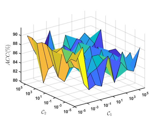
(a) Chimpanzee vs Giant panda

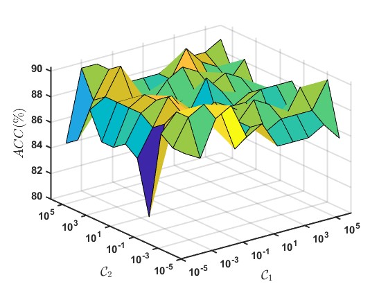
(b) Giant panda vs Leopard

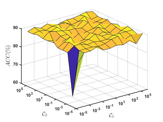
(c) Persian cat vs Rat

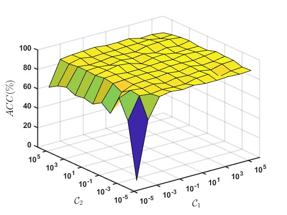
(d) Giant panda vs Hippopotamus

Figure 10: Effect of parameter $\mathcal{C}_{1}$ and $\mathcal{C}_{2}$ on the performance of the proposed MvRVFL model on AwA dataset.

A.2.2 Performance with different number of training samples on AwA dataset

We assess how the proposed MvRVFL model’s performance varies with different numbers of training samples. Fig. 11 shows how the Acc. changes as the number of training samples ranges from $86$ to $336$. The x-axis displays the number of training samples, and the y-axis shows the corresponding Acc. values. It is observed that the Acc. value generally increases with the rise in the number of training samples. This is because an increase in training samples provides more data for the model to learn from, leading to improved accuracy in the classification results.

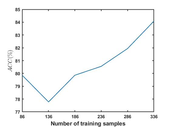
(a) Chimpanzee vs
Giant panda

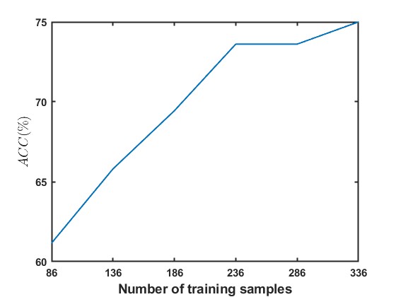
(b) Chimpanzee panda vs
Hippopotamus

(c) Chimpanzee vs
Seal

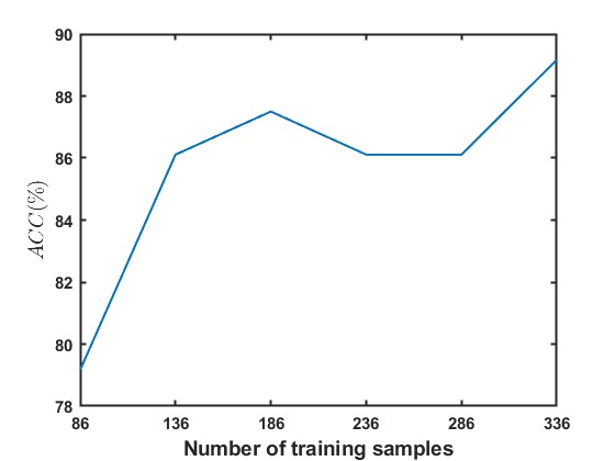
(d) Giant panda vs
Leopard

Figure 11: Performance with different number of training samples of the proposed MvRVFL model on AwA dataset.

A.3 Effect of hyperparameters $C_{1}$ and $\sigma$

A.3.1 Sensitivity of $\theta$ and $\rho$ combinations

We explore the sensitivity of the MvRVFL model to various values of parameters $\theta$ and $\rho$. The parameter $\theta$ regulates the gap between two views, while $\rho$ is linked to the coupling term $\xi_{1}^{t}\xi_{2}$. We vary the values of $\theta$ and $\rho$ from $10^{-5}$ to $10^{5}$ and record the corresponding Acc. results. With other parameters held constant at their optimal settings, Fig. 12 illustrates how the performance of MvRVFL changes as the values of parameters $\theta$ and $\rho$ are varied.

From the perspective of hyperparameters, $\theta$ and $\rho$, the parameter $\theta$ regulates the gap between view $A$ and view $B$. With the same value of $\rho$, when $\theta>10^{-1}$, it indicates that view $B$ plays a more significant role than view $A$ in learning the overall model. Otherwise, view $A$ is more important. For instance, on the 1000 and 10000 sub-datasets, the Acc. reaches its highest value when the parameter $\theta$ is relatively large (e.g., $10^{3}$ or $10^{5}$), suggesting that view $B$ holds greater importance than view $A$. Furthermore, on the 103000, and 143000 sub-datasets, the optimal performance is achieved when the parameter $\theta$ is small (e.g., $10^{-5}$ or $10^{-3}$), indicating that view $A$ holds more significance than view $B$.

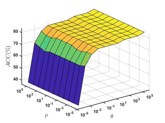
(a) 1000

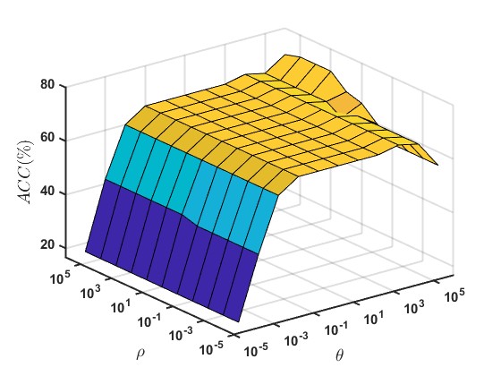
(b) 10000

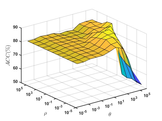
(c) 103000

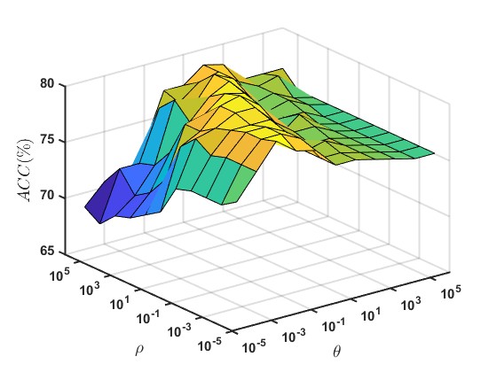
(d) 143000

Figure 12: Performance variation with different values of parameters $\theta$ and $\rho$ of the proposed MvRVFL model on Corel5k dataset.

A.4 Classification accuracy tables of the proposed MvRVFL models along with baseline models on UCI, KEEL, AwA and Corel5k datasets

In this section, we present the performance of the proposed MvRVFL models, along with the baseline models.

Table 7: Performance comparison of the proposed MvRVFL along with the baseline models based on classification Acc. for UCI and KEEL datasets.

Dataset	SVM2K	MvTSVM	ELM-Vw-$A$	ELM-Vw-$B$	RVFL-Vw-$A$	RVFL-Vw-$B$	MVLDM	MvRVFL-1†	MvRVFL-2†
	(Farquhar et al., 2005)	(Xie & Sun, 2015)	(Huang et al., 2006)	(Huang et al., 2006)	(Pao et al., 1994)	(Pao et al., 1994)	(Hu et al., 2024)
	$(C_{1})$	$(C_{1},C_{2},D)$	$(C,N)$	$(C,N)$	$(C,N)$	$(C,N)$	$(C_{1},\nu_{1},\nu_{2},\sigma)$	$(C_{1},C_{2},\rho,N)$	$(C_{1},C_{2},\rho,N)$
aus	$87.02$	$71.15$	$85.98$	$86.06$	$85.98$	$85.98$	$71.98$	$87.5$	$87.98$
	$(0.001)$	$(0.00001,0.00001,0.00001)$	$(0.01,123)$	$(0.001,163)$	$(0.001,163)$	$(10,23)$	$(0.001,0.01,0.1,0.25)$	$(1,0.0001,0.00001,63)$	$(100,100000,1,43)$
bank	$80.74$	$71.86$	$85.54$	$85.39$	$85.83$	$85.61$	$73.67$	$90.05$	$89.24$
	$(0.001)$	$(0.00001,0.00001,0.00001)$	$(0.00001,3)$	$(10000,23)$	$(1000,163)$	$(10,123)$	$(0.1,0.001,0.001,4)$	$(100,0.1,0.0001,203)$	$(100,1000,0.0001,83)$
breast_cancer	$62.45$	$55.58$	$69.77$	$65.12$	$67.44$	$66.28$	$70$	$70.93$	$75.58$
	$(0.001)$	$(0.00001,0.00001,0.00001)$	$(1,83)$	$(0.01,43)$	$(0.0001,3)$	$(1,83)$	$(0.0001,0.1,0.001,4)$	$(0.1,0.0001,0.00001,43)$	$(0.0001,0.01,0.0001,43)$
breast_cancer_wisc	$90.04$	$81.43$	$92.1$	$92.1$	$92.14$	$95.1$	$75$	$98.57$	$96.19$
	$(0.00001)$	$(0.00001,0.00001,0.00001)$	$(0.0001,203)$	$(0.01,63)$	$(0.00001,23)$	$(0.0001,203)$	$(0.0001,0.0001,0.00001,0.25)$	$(0.00001,0.1,0.00001,163)$	$(100,0.001,10,23)$
breast_cancer_wisc_diag	$95.49$	$88.6$	$92.42$	$97.08$	$95.83$	$96.49$	$93.15$	$98.25$	$97.08$
	$(0.001)$	$(0.00001,0.00001,0.00001)$	$(0.01,163)$	$(0.001,163)$	$(0.001,163)$	$(100,3)$	$(0.001,0.0001,1,4)$	$(0.001,0.0001,0.0001,123)$	$(0.1,10,0.0001,83)$
breast_cancer_wisc_prog	$58.33$	$58.33$	$68.33$	$68.33$	$73.33$	$68.33$	$71.17$	$73.33$	$73.33$
	$(0.001)$	$(0.00001,0.00001,0.00001)$	$(0.01,203)$	$(0.01,83)$	$(100000,3)$	$(0.01,203)$	$(0.0001,0.0001,0.1,2)$	$(1,10,0.00001,23)$	$(10000,100,100,3)$
brwisconsin	$97.56$	$61.95$	$97.07$	$96.1$	$97.07$	$96.59$	$95.59$	$96.1$	$97.56$
	$(0.00001)$	$(0.00001,0.00001,0.00001)$	$(0.0001,143)$	$(0.001,63)$	$(0.001,63)$	$(100000,23)$	$(0.001,0.00001,0.1,4)$	$(0.00001,1,0.001,163)$	$(0.0001,1,0.00001,203)$
bupa or liver-disorders	$54.8$	$42.31$	$63.46$	$65.38$	$63.46$	$66.35$	$55.34$	$70.19$	$64.42$
	$(0.00001)$	$(0.00001,0.00001,0.00001)$	$(1000,23)$	$(0.1,163)$	$(0.1,163)$	$(0.1,163)$	$(0.001,0.001,0.001,4)$	$(10,0.01,0.001,23)$	$(0.1,1,0.0001,83)$
checkerboard_Data	$87.02$	$43.75$	$86.98$	$86.06$	$86.98$	$86.98$	$84.06$	$87.5$	$87.98$
	$(0.00001)$	$(0.00001,0.00001,0.00001)$	$(0.01,123)$	$(0.001,163)$	$(0.001,163)$	$(10,23)$	$(0.001,0.001,0.001,1)$	$(1,0.0001,0.00001,63)$	$(100,100000,1,43)$
chess_krvkp	$80.45$	$82.35$	$95.62$	$93.33$	$95.62$	$94.68$	$97.7$	$96.77$	$94.58$
	$(0.001)$	$(0.00001,0.00001,0.00001)$	$(100,203)$	$(100000,203)$	$(10000,203)$	$(100,203)$	$(0.1,0.1,0.1,4)$	$(0.1,0.0001,0.1,203)$	$(100000,0.00001,10,203)$
cleve	$80$	$75.56$	$80$	$85.56$	$81.11$	$81.11$	$84.27$	$84.44$	$81.11$
	$(0.1)$	$(0.00001,0.00001,0.00001)$	$(0.001,103)$	$(0.001,123)$	$(0.01,3)$	$(0.01,23)$	$(0.01,0.0.1,0.1,1)$	$(0.00001,1,0.00001,203)$	$(0.0001,0.1,0.00001,123)$
cmc	$64.25$	$55.88$	$69.91$	$70.14$	$68.1$	$71.72$	$74.38$	$72.17$	$70.36$
	$(0.00001)$	$(0.00001,0.00001,0.00001)$	$(0.01,143)$	$(0.01,183)$	$(100,63)$	$(1000,43)$	$(0.0001,0.01,0.001,4)$	$(1000,1,0.001,23)$	$(10000,0.00001,0.0001,23)$
conn_bench_sonar_mines_rocks	$80.95$	$46.03$	$80.54$	$74.6$	$88.54$	$73.02$	$75.81$	$80.95$	$66.67$
	$(1000)$	$(0.00001,0.00001,0.00001)$	$(10,3)$	$(0.01,203)$	$(0.01,203)$	$(0.1,183)$	$(0.0001,0.00001,10,0.5)$	$(10,1000,0.1,183)$	$(10,1000,10,163)$
cylinder_bands	$68.18$	$60.39$	$76.62$	$74.03$	$72.08$	$74.68$	$71.9$	$74.68$	$78.57$
	$(0.00001)$	$(0.00001,0.00001,0.00001)$	$(0.001,203)$	$(100,143)$	$(0.001,183)$	$(1,23)$	$(0.0001,0.1,0.001,4)$	$(100,0.01,0.0001,43)$	$(10,1000,0.01,43)$
fertility	$75.25$	$75$	$90$	$90$	$90$	$90$	$86.67$	$93.33$	$86.67$
	$(0.01)$	$(0.00001,0.00001,0.00001)$	$(0.01,83)$	$(0.01,63)$	$(0.01,63)$	$(0.01,83)$	$(0.001,0.001,100,2)$	$(0.01,1,0.01,183)$	$(0.0001,10000,1,63)$
hepatitis	$80.85$	$78.72$	$78.85$	$80.85$	$80.85$	$78.72$	$78.26$	$85.11$	$78.72$
	$(0.00001)$	$(0.00001,0.00001,0.00001)$	$(1,23)$	$(0.01,183)$	$(0.1,123)$	$(10,3)$	$(0.001,0.01,0.001,4)$	$(0.01,100,0.00001,203)$	$(0.01,100,0.00001,203)$
hill_valley	$60.98$	$53.3$	$68.05$	$51.92$	$68.78$	$51.92$	$56.2$	$68.96$	$75.89$
	$(0.00001)$	$(0.00001,0.00001,0.00001)$	$(10000,103)$	$(1,103)$	$(10,103)$	$(10000,103)$	$(0.0001,0.0001,0.1,1)$	$(10,0.1,0.0001,123)$	$(100,1,100,143)$
mammographic	$80.27$	$77.06$	$80.28$	$82.01$	$80.28$	$81.66$	$83.33$	$84.08$	$83.74$
	$(0.01)$	$(0.00001,0.00001,0.00001)$	$(1,83)$	$(100000,63)$	$(100000,23)$	$(100,23)$	$(0.0001,0.001,1,4)$	$(1000,1,0.00001,23)$	$(1000,0.00001,0.0001,23)$
monks_3	$80.24$	$76.11$	$95.21$	$95.41$	$95.21$	$95.81$	$96.39$	$96.41$	$96.41$
	$(0.01)$	$(0.00001,0.00001,0.00001)$	$(0.1,143)$	$(0.1,163)$	$(0.1,163)$	$(0.1,123)$	$(0.01,0.001,10,4)$	$(0.1,0.00001,0.001,163)$	$(0.1,1,0.00001,183)$
new-thyroid1	$78.46$	$82.31$	$98.46$	$96.92$	$98.46$	$96.92$	$95.31$	$100$	$100$
	$(0.1)$	$(0.00001,0.00001,0.00001)$	$(10,103)$	$(1,43)$	$(1,23)$	$(10,103)$	$(0.0001,1000,0.1,0.25)$	$(0.001,0.0001,0.00001,183)$	$(1,0.001,0.01,123)$
oocytes_merluccius_nucleus_4d	$74.27$	$64.82$	$82.41$	$81.11$	$83.71$	$80.78$	$75.16$	$82.08$	$81.76$
	$(0.00001)$	$(0.00001,0.00001,0.00001)$	$(0.1,83)$	$(1,143)$	$(1,143)$	$(0.1,83)$	$(0.1,100,0.1,4)$	$(10,100,0.1,143)$	$(1,10000,0.001,203)$
oocytes_trisopterus_nucleus_2f	$78.83$	$58.39$	$86.13$	$78.83$	$85.04$	$78.83$	$82.05$	$85.04$	$86.5$
	$(0.0001)$	$(0.00001,0.00001,0.00001)$	$(0.01,103)$	$(0.1,143)$	$(100000,43)$	$(0.01,103)$	$(0.1,0.001,1,4)$	$(100000,0.0001,100,83)$	$(0.1,100,0.1,203)$
parkinsons	$71.19$	$71.19$	$81.36$	$77.97$	$89.83$	$77.97$	$93.1$	$89.83$	$93.22$
	$(0.01)$	$(0.00001,0.00001,0.00001)$	$(0.1,163)$	$(1,63)$	$(0.1,203)$	$(0.1,163)$	$(0.0001,0.00001,1,2)$	$(1000,100000,0.1,163)$	$(1,1000,0.01,203)$
pima	$76.19$	$73.33$	$74.89$	$74.03$	$74.46$	$74.03$	$69.13$	$76.19$	$74.89$
	$(0.01)$	$(0.00001,0.00001,0.00001)$	$(0.1,63)$	$(0.01,143)$	$(0.01,143)$	$(0.1,63)$	$(0.0001,10,10,4)$	$(0.001,1,0.01,3)$	$(10000,0.01,0.001,3)$
pittsburg_bridges_T_OR_D	$70.85$	$65.85$	$89.32$	$73.55$	$80.65$	$80.65$	$90$	$90.32$	$74.19$
	$(100)$	$(0.00001,0.00001,0.00001)$	$(0.01,83)$	$(0.01,43)$	$(1000,3)$	$(0.01,3)$	$(0.1,0.00001,1,4)$	$(0.00001,1,0.01,163)$	$(10000,10,0.0001,3)$
planning	$65.85$	$63.64$	$76.36$	$76.36$	$76.36$	$76.36$	$68.52$	$76.36$	$63.64$
	$(10)$	$(0.00001,0.00001,0.00001)$	$(0.01,23)$	$(0.00001,3)$	$(0.00001,23)$	$(0.01,23)$	$(0.00001,0.001,1,1)$	$(0.01,0.00001,0.0001,23)$	$(0.0001,0.01,100000,43)$
ripley	$89.07$	$80.67$	$86.13$	$87.53$	$87.53$	$87.53$	$89.07$	$89.87$	$89.6$
	$(100000)$	$(0.00001,0.00001,0.00001)$	$(10000,103)$	$(100,203)$	$(10000,123)$	$(10000,103)$	$(0.001,0.001,0.001,4)$	$(1,0.00001,0.0001,123)$	$(10000,0.01,10,83)$
Average Acc.	$76.65$	$67.24$	$82.66$	$80.95$	$83.14$	$81.26$	$79.9$	$85.15$	$83.18$
Average Rank	$6.35$	$8.65$	$4.70$	$5.26$	$4.22$	$5.09$	$5.48$	$2.04$	$3.20$
† represents the proposed models.

Table 8: Performance comparison of the proposed MvRVFL along with the baseline models based on classification Acc. for AwA datasets.

Dataset	SVM2K	MvTSVM	ELM-Vw-$A$	ELM-Vw-$B$	RVFL-Vw-$A$	RVFL-Vw-$B$	MVLDM	MvRVFL-1†	MvRVFL-2†
	(Farquhar et al., 2005)	(Xie & Sun, 2015)	(Huang et al., 2006)	(Huang et al., 2006)	(Pao et al., 1994)	(Pao et al., 1994)	(Hu et al., 2024)
	$(C_{1})$	$(C_{1},C_{2},D)$	$(C,N)$	$(C,N)$	$(C,N)$	$(C,N)$	$(C_{1},\nu_{1},\nu_{2},\sigma)$	$(C_{1},C_{2},\rho,N)$	$(C_{1},C_{2},\rho,N)$
Chimpanzee vs Giant panda	$84.03$	$47.22$	$71.53$	$72.92$	$71.53$	$80.89$	$72.22$	$88.19$	$84.72$
	$(0.00001)$	$(0.00001,0.00001,0.00001)$	$(0.0001,123)$	$(0.00001,163)$	$(0.001,3)$	$(0.001,3)$	$(1000,0.0001,0.01,4)$	$(100,100000,0.01,3)$	$(0.001,10,0.0001,3)$
Chimpanzee vs Leopard	$80.11$	$46.53$	$63.89$	$83.33$	$72.92$	$80.42$	$68.75$	$89.58$	$84.72$
	$(0.00001)$	$(0.00001,0.00001,0.00001)$	$(1000,43)$	$(0.00001,203)$	$(0.01,23)$	$(0.0001,3)$	$(0.001,0.00001,0.00001,4)$	$(0.001,1,0.00001,3)$	$(0.001,1,0.00001,3)$
Chimpanzee vs Persian cat	$70.86$	$50$	$79.86$	$69.44$	$79.17$	$80.56$	$86.11$	$83.33$	$74.31$
	$(0.0001)$	$(0.00001,0.00001,0.00001)$	$(0.0001,183)$	$(0.00001,183)$	$(0.0001,183)$	$(0.1,3)$	$(100,0.0001,0.00001,4)$	$(0.001,1,0.00001,3)$	$(0.001,1,0.001,23)$
Chimpanzee vs Pig	$50.42$	$51.39$	$68.75$	$81.25$	$69.44$	$79.17$	$66.67$	$61.81$	$80.56$
	$(0.01)$	$(0.00001,0.00001,0.00001)$	$(0.00001,163)$	$(0.00001,163)$	$(0.00001,163)$	$(10,3)$	$(100000,0.001,0.001,4)$	$(0.1,10000,100000,23)$	$(0.001,1,0.00001,3)$
Chimpanzee vs Hippopotamus	$70.94$	$54.86$	$71.53$	$70.14$	$72.92$	$78.47$	$78.47$	$79.17$	$75$
	$(0.00001)$	$(0.00001,0.00001,0.00001)$	$(0.00001,143)$	$(0.00001,183)$	$(0.00001,143)$	$(0.001,3)$	$(1000,0.0001,1,4)$	$(0.0001,0.1,0.00001,3)$	$(0.001,1,0.00001,3)$
Chimpanzee vs Humpback whale	$92.36$	$81.39$	$86.81$	$92.36$	$88.89$	$91.14$	$81.25$	$95.14$	$93.06$
	$(0.1)$	$(0.00001,0.00001,0.00001)$	$(0.0001,83)$	$(0.00001,183)$	$(0.0001,83)$	$(0.01,3)$	$(10000,0.001,0.0001,4)$	$(0.001,0.01,0.00001,23)$	$(0.001,10,0.00001,3)$
Chimpanzee vs Raccoon	$80.33$	$63.47$	$69.44$	$63.89$	$73.61$	$79.86$	$72.22$	$83.33$	$82.64$
	$(0.001)$	$(0.00001,0.00001,100000)$	$(0.0001,203)$	$(0.00001,123)$	$(0.001,3)$	$(1000,23)$	$(10000,0.00001,0.01,4)$	$(0.001,1,0.0001,3)$	$(0.001,1,0.00001,3)$
Chimpanzee vs Rat	$77.08$	$52.78$	$57.64$	$75$	$63.89$	$71.94$	$68.06$	$81.25$	$78.47$
	$(10)$	$(0.00001,0.00001,0.00001)$	$(100000,43)$	$(0.00001,183)$	$(0.001,163)$	$(0.001,3)$	$(100000,0.0001,0.00001,4)$	$(0.1,1,0.01,43)$	$(0.00001,0.0001,0.00001,63)$
Chimpanzee vs Seal	$70.69$	$53.47$	$79.17$	$76.39$	$79.17$	$79.81$	$75.69$	$83.33$	$78.47$
	$(0.01)$	$(0.00001,0.00001,0.00001)$	$(0.0001,183)$	$(0.00001,143)$	$(0.001,3)$	$(0.0001,3)$	$(0.001,0.001,0.01,0.25)$	$(10,10000,0.001,23)$	$(0.01,10,0.0001,3)$
Giant panda vs Leopard	$80.19$	$54.17$	$61.11$	$78.47$	$72.92$	$80.11$	$61.81$	$88.89$	$83.33$
	$(0.01)$	$(0.00001,0.00001,0.00001)$	$(0.0001,103)$	$(0.00001,203)$	$(0.001,3)$	$(0.001,3)$	$(100000,0.00001,0.01,0.25)$	$(0.001,1,0.001,3)$	$(100,0.01,100,63)$
Giant panda vs Persian cat	$81.81$	$52.08$	$77.78$	$76.39$	$64.58$	$80.42$	$66.67$	$85.42$	$81.94$
	$(0.0001)$	$(0.00001,0.00001,0.00001)$	$(100,103)$	$(0.00001,203)$	$(0.001,23)$	$(100000,3)$	$(0.01,0.00001,0.01,4)$	$(0.001,0.1,0.00001,23)$	$(1000,0.01,1000,23)$
Giant panda vs Pig	$80.56$	$51.39$	$63.89$	$75$	$65.97$	$79.81$	$65.97$	$84.72$	$83.33$
	$(0.0001)$	$(0.00001,0.00001,0.00001)$	$(1,43)$	$(0.00001,203)$	$(0.001,3)$	$(0.001,3)$	$(1000,0.00001,0.01,0.25)$	$(1,0.1,0.1,23)$	$(0.00001,0.01,0.00001,23)$
Giant panda vs Hippopotamus	$77.78$	$54.17$	$74.31$	$81.25$	$68.06$	$71.94$	$74.31$	$83.33$	$75$
	$(0.01)$	$(0.00001,0.00001,0.00001)$	$(0.00001,183)$	$(0.00001,183)$	$(0.01,3)$	$(0.01,23)$	$(100000,0.001,100,2)$	$(0.01,1,0.00001,23)$	$(0.001,0.00001,0.00001,43)$
Giant panda vs Humpback whale	$93.06$	$46.53$	$93.06$	$91.67$	$93.06$	$93.22$	$93.75$	$95.83$	$94.44$
	$(0.00001)$	$(0.00001,0.00001,0.00001)$	$(0.0001,203)$	$(0.00001,203)$	$(0.0001,203)$	$(0.001,3)$	$(0.001,0.00001,0.01,4)$	$(0.001,0.0001,0.0001,3)$	$(0.01,100,0.0001,3)$
Giant panda vs Raccoon	$80.19$	$52.78$	$68.06$	$74.31$	$68.75$	$80.19$	$64.58$	$84.72$	$78.47$
	$(10000)$	$(0.00001,0.00001,0.00001)$	$(0.0001,203)$	$(0.00001,163)$	$(0.00001,203)$	$(0.001,3)$	$(100000,0.00001,0.00001,2)$	$(0.001,10,0.0001,3)$	$(0.001,10,0.0001,3)$
Giant panda vs Rat	$83.33$	$69.31$	$66.67$	$76.39$	$68.06$	$80.5$	$70.14$	$86.81$	$81.25$
	$(1)$	$(0.00001,0.00001,100000)$	$(10,103)$	$(0.00001,123)$	$(0.001,43)$	$(0.001,3)$	$(10000,0.0001,0.01,0.25)$	$(0.001,1,0.0001,3)$	$(0.001,1,0.00001,3)$
Giant panda vs Seal	$85.89$	$56.94$	$80.56$	$77.08$	$80.56$	$80.19$	$86.81$	$91.67$	$79.17$
	$(0.1)$	$(0.00001,0.00001,0.00001)$	$(0.0001,203)$	$(0.00001,183)$	$(0.001,3)$	$(0.0001,3)$	$(100000,0.001,0.01,2)$	$(0.01,0.01,0.00001,3)$	$(0.001,0.001,0.0001,23)$
Leopard vs Persian cat	$82.19$	$79.31$	$70.83$	$84.72$	$77.78$	$88.19$	$80.56$	$90.97$	$85.42$
	$(0.00001)$	$(0.00001,0.00001,0.00001)$	$(100,63)$	$(0.00001,203)$	$(0.001,23)$	$(0.001,3)$	$(0.00001,0.00001,100,4)$	$(0.001,1,0.001,3)$	$(0.00001,10,0.00001,163)$
Leopard vs Pig	$75$	$61.39$	$61.11$	$75$	$66.67$	$72.17$	$68.75$	$78.47$	$75$
	$(0.01)$	$(0.00001,0.00001,0.00001)$	$(0.0001,183)$	$(0.00001,183)$	$(0.001,3)$	$(0.001,3)$	$(0.01,0.001,100,4)$	$(0.001,1,0.0001,3)$	$(0.1,0.00001,0.1,23)$
Leopard vs Hippopotamus	$78.17$	$50.69$	$73.61$	$77.08$	$74.31$	$75.94$	$75$	$81.94$	$76.39$
	$(10)$	$(0.00001,0.00001,0.00001)$	$(0.0001,143)$	$(0.00001,143)$	$(0.0001,43)$	$(0.0001,3)$	$(10000,0.0001,0.001,4)$	$(0.001,0.00001,0.00001,3)$	$(0.00001,10,0.00001,183)$
Leopard vs Humpback whale	$90.75$	$79.31$	$89.58$	$91.67$	$90.97$	$90.83$	$89.58$	$93.75$	$88.19$
	$(0.00001)$	$(0.00001,0.00001,0.00001)$	$(0.00001,103)$	$(0.00001,183)$	$(0.0001,143)$	$(0.001,23)$	$(100,0.00001,0.01,4)$	$(0.1,100,0.0001,43)$	$(0.0001,0.001,0.0001,63)$
Leopard vs Raccoon	$80.56$	$55$	$59.03$	$57.64$	$59.03$	$69.25$	$56.94$	$84.03$	$70.14$
	$(0.0001)$	$(0.00001,0.00001,0.00001)$	$(0.0001,183)$	$(0.0001,183)$	$(0.001,3)$	$(0.001,3)$	$(0.01,0.00001,0.00001,0.25)$	$(0.001,0.00001,0.00001,3)$	$(0.0001,0.1,0.00001,3)$
Leopard vs Rat	$76.42$	$68.61$	$72.22$	$76.39$	$68.06$	$79.86$	$65.28$	$79.17$	$80.56$
	$(0.0001)$	$(0.00001,0.00001,0.00001)$	$(10000,43)$	$(0.00001,183)$	$(0.001,3)$	$(0.001,3)$	$(10000,0.0001,0.00001,0.25)$	$(100,100000,1,3)$	$(0.00001,0.01,0.00001,23)$
Leopard vs Seal	$80.42$	$63.47$	$75.69$	$79.86$	$75$	$83.33$	$81.25$	$84.03$	$78.47$
	$(10000)$	$(0.00001,0.00001,0.00001)$	$(0.0001,123)$	$(0.00001,143)$	$(0.0001,123)$	$(0.001,43)$	$(10000,0.0001,0.0001,4)$	$(0.01,100,0.0001,23)$	$(0.0001,0.0001,0.00001,3)$
Persian cat vs Pig	$70$	$69.31$	$63.89$	$67.36$	$70.14$	$74.31$	$69.44$	$74.31$	$71.53$
	$(0.001)$	$(0.00001,0.00001,0.00001)$	$(0.0001,183)$	$(0.00001,163)$	$(0.001,3)$	$(10000,3)$	$(100,0.00001,0.01,4)$	$(0.01,10,0.00001,3)$	$(0.01,10,0.001,3)$
Persian cat vs Hippopotamus	$76.81$	$76.53$	$75.69$	$79.86$	$77.08$	$78.94$	$75.69$	$83.33$	$79.86$
	$(0.01)$	$(0.00001,0.00001,0.00001)$	$(1,63)$	$(0.00001,203)$	$(0.01,3)$	$(1,3)$	$(100000,0.001,0.00001,0.25)$	$(0.0001,0.00001,0.00001,3)$	$(0.01,0.00001,0.001,3)$
Persian cat vs Humpback whale	$71.67$	$71.39$	$81.25$	$88.19$	$81.94$	$81.75$	$85.42$	$94.44$	$82.64$
	$(0.00001)$	$(0.00001,0.00001,0.00001)$	$(0.00001,143)$	$(0.00001,203)$	$(0.00001,143)$	$(1,23)$	$(0.01,0.00001,0.1,4)$	$(10000,1,10000,23)$	$(0.001,0.1,0.0001,23)$
Persian cat vs Raccoon	$82.64$	$79.31$	$73.61$	$81.25$	$69.44$	$71.64$	$65.97$	$84.03$	$73.61$
	$(0.00001)$	$(0.00001,0.00001,0.00001)$	$(100,23)$	$(0.00001,163)$	$(0.001,23)$	$(0.001,3)$	$(100000,0.00001,0.001,2)$	$(1,10000,0.01,3)$	$(0.00001,100000,0.00001,3)$
Persian cat vs Rat	$60.44$	$64.17$	$54.86$	$56.25$	$59.72$	$60.67$	$56.94$	$61.11$	$63.89$
	$(0.001)$	$(0.00001,0.00001,0.00001)$	$(0.001,183)$	$(100000,103)$	$(0.001,3)$	$(0.001,3)$	$(1000,0.00001,10,0.5)$	$(0.0001,0.0001,0.00001,63)$	$(0.001,1,0.00001,3)$
Persian cat vs Seal	$80.42$	$73.47$	$72.22$	$71.53$	$65.97$	$72.94$	$83.33$	$84.72$	$76.39$
	$(1)$	$(0.00001,0.00001,0.00001)$	$(0.0001,183)$	$(0.00001,83)$	$(0.01,63)$	$(0.001,3)$	$(10000,0.00001,0.01,4)$	$(0.01,100,0.001,3)$	$(0.01,100,0.00001,3)$
Pig vs Hippopotamus	$71.53$	$65.83$	$70.14$	$65.97$	$64.58$	$67.36$	$72.22$	$71.53$	$64.58$
	$(0.0001)$	$(0.00001,0.00001,0.00001)$	$(0.0001,83)$	$(0.00001,203)$	$(0.0001,123)$	$(0.01,63)$	$(1000,0.00001,0.01,0.25)$	$(0.01,100,0.001,3)$	$(0.0001,10,0.00001,163)$
Pig vs Humpback whale	$80.19$	$77.92$	$82.64$	$89.58$	$82.64$	$80.19$	$88.89$	$90.28$	$84.72$
	$(0.01)$	$(0.00001,0.00001,0.00001)$	$(0.00001,203)$	$(0.00001,203)$	$(0.00001,203)$	$(0.001,3)$	$(100000,0.001,0.0001,0.25)$	$(0.01,10,0.01,3)$	$(0.00001,10,0.00001,143)$
Pig vs Raccoon	$71.69$	$69.31$	$61.11$	$72.92$	$64.58$	$72.22$	$62.5$	$80.56$	$72.33$
	$(0.00001)$	$(0.00001,0.00001,0.00001)$	$(0.0001,43)$	$(0.00001,183)$	$(0.0001,43)$	$(10000,3)$	$(0.0001,0.00001,0.0001,4)$	$(0.001,1,0.00001,3)$	$(0.0001,0.01,0.0001,23)$
Pig vs Rat	$71.53$	$68.61$	$62.5$	$59.72$	$57.64$	$68.06$	$64.58$	$64.58$	$69.72$
	$(0.01)$	$(0.00001,0.00001,0.00001)$	$(1000,63)$	$(0.0001,203)$	$(0.001,43)$	$(0.001,3)$	$(1000,0.00001,0.01,0.25)$	$(100,10000,0.001,43)$	$(0.00001,1,0.00001,143)$
Pig vs Seal	$72.69$	$65.56$	$70.14$	$68.06$	$72.92$	$74.31$	$72.92$	$78.47$	$74.31$
	$(0.01)$	$(0.00001,0.00001,0.00001)$	$(0.00001,163)$	$(0.00001,183)$	$(0.001,3)$	$(0.0001,3)$	$(0.001,0.001,0.00001,4)$	$(0.001,1,0.00001,3)$	$(0.001,10,0.0001,3)$
Hippopotamus vs Humpback whale	$82.03$	$80.31$	$77.78$	$79.86$	$81.25$	$82.81$	$79.86$	$88.19$	$83.33$
	$(0.01)$	$(0.00001,0.00001,0.00001)$	$(0.0001,143)$	$(0.00001,143)$	$(0.01,3)$	$(0.001,23)$	$(0.001,0.0001,10000,0.25)$	$(0.01,10,0.00001,43)$	$(0.001,10,0.00001,3)$
Hippopotamus vs Raccoon	$78.47$	$75.14$	$72.22$	$70.14$	$78.47$	$80.94$	$75.69$	$81.94$	$77.78$
	$(0.01)$	$(0.00001,0.00001,0.00001)$	$(0.0001,203)$	$(0.00001,183)$	$(0.001,3)$	$(0.001,23)$	$(0.00001,0.001,1,4)$	$(0.01,10,0.00001,23)$	$(0.001,1,0.0001,3)$
Hippopotamus vs Rat	$75.33$	$75.83$	$65.28$	$71.53$	$70.14$	$70.25$	$64.58$	$81.25$	$75$
	$(100)$	$(0.00001,0.00001,0.00001)$	$(1000,43)$	$(0.00001,183)$	$(0.01,23)$	$(0.001,3)$	$(100000,0.0001,0.1,4)$	$(0.01,10,0.01,3)$	$(0.00001,0.01,0.00001,43)$
Hippopotamus vs Seal	$69.44$	$49.31$	$58.33$	$65.28$	$61.81$	$70.83$	$60.42$	$59.03$	$61.81$
	$(0.01)$	$(0.00001,0.00001,0.00001)$	$(0.1,63)$	$(0.00001,183)$	$(0.001,43)$	$(0.001,3)$	$(0.001,0.01,0.00001,4)$	$(1,1,1,23)$	$(0.0001,0.1,0.00001,63)$
Humpback whale vs Raccoon	$85.67$	$80.69$	$84.03$	$90.97$	$81.94$	$82.36$	$83.33$	$90.28$	$83.33$
	$(0.00001)$	$(0.00001,0.00001,10000)$	$(0.00001,83)$	$(0.00001,123)$	$(0.0001,83)$	$(0.001,3)$	$(10000,0.0001,0.01,0.25)$	$(0.001,0.001,0.0001,43)$	$(0.0001,0.0001,0.00001,3)$
Humpback whale vs Rat	$82.28$	$80.31$	$81.94$	$86.11$	$81.94$	$80.58$	$77.78$	$91.67$	$84.72$
	$(0.01)$	$(0.00001,0.00001,0.00001)$	$(0.0001,183)$	$(0.00001,203)$	$(0.0001,183)$	$(100,3)$	$(100000,0.001,10,0.25)$	$(10,10000,0.1,23)$	$(0.00001,0.001,0.00001,3)$
Humpback whale vs Seal	$76.39$	$72.08$	$77.78$	$73.61$	$78.47$	$79.17$	$78.47$	$78.47$	$71.53$
	$(0.01)$	$(0.00001,0.00001,0.00001)$	$(0.0001,143)$	$(0.00001,203)$	$(0.0001,143)$	$(0.0001,3)$	$(100000,0.0001,0.001,0.25)$	$(0.001,0.1,0.0001,3)$	$(100,0.01,100,23)$
Raccoon vs Rat	$62.22$	$61.89$	$59.72$	$70.83$	$61.81$	$60.22$	$65.28$	$68.75$	$66.67$
	$(100)$	$(0.00001,0.00001,0.00001)$	$(100,43)$	$(0.00001,163)$	$(0.001,163)$	$(0.001,3)$	$(100000,0.00001,10,4)$	$(0.1,10,0.1,3)$	$(0.0001,0.01,0.0001,43)$
Raccoon vs Seal	$90.28$	$75.39$	$78.47$	$84.03$	$82.64$	$80.28$	$75.69$	$88.89$	$79.86$
	$(100)$	$(0.00001,0.00001,100000)$	$(0.00001,183)$	$(0.00001,183)$	$(0.001,63)$	$(0.001,3)$	$(100000,0.00001,0.01,4)$	$(0.001,0.00001,0.0001,23)$	$(0.01,100,0.00001,3)$
Rat vs Seal	$70.86$	$65.17$	$68.75$	$68.75$	$68.75$	$67.83$	$69.87$	$77.78$	$68.06$
	$(0.001)$	$(0.00001,0.00001,0.00001)$	$(0.00001,183)$	$(0.00001,143)$	$(0.00001,183)$	$(0.01,3)$	$(100000,0.001,0.01,0.25)$	$(0.01,10,0.001,3)$	$(0.001,0.00001,0.00001,23)$
Average Acc.	$77.46$	$64.31$	$71.74$	$75.99$	$72.87$	$77.46$	$73.33$	$82.5$	$77.97$
Average Rank	$4.08$	$7.71$	$6.82$	$4.9$	$6.06$	$4.26$	$5.74$	$1.63$	$3.8$
† represents the proposed models.

Table 9: Performance comparison of the proposed MvRVFL along with the baseline models based on classification Acc. for Corel5k datasets.

Dataset	SVM2K	MvTSVM	ELM-Vw-$A$	ELM-Vw-$B$	RVFL-Vw-$A$	RVFL-Vw-$B$	MVLDM	MvRVFL-1†	MvRVFL-2†
	(Farquhar et al., 2005)	(Xie & Sun, 2015)	(Huang et al., 2006)	(Huang et al., 2006)	(Pao et al., 1994)	(Pao et al., 1994)	(Hu et al., 2024)
	$(C_{1})$	$(C_{1},C_{2},D)$	$(C,N)$	$(C,N)$	$(C,N)$	$(C,N)$	$(C_{1},\nu_{1},\nu_{2},\sigma)$	$(C_{1},C_{2},\rho,N)$	$(C_{1},C_{2},\rho,N)$
1000	$81.67$	$50$	$83.33$	$78.33$	$83.33$	$76.67$	$73.33$	$83.33$	$85$
	$(0.0625)$	$(0.00001,0.00001,0.00001)$	$(0.0001,183)$	$(0.00001,43)$	$(0.0001,183)$	$(0.00001,3)$	$(0.01,0.001,0.001,4)$	$(0.001,0.01,0.00001,23)$	$(0.0001,100000,0.00001,203)$
10000	$71.67$	$48.33$	$56.67$	$63.33$	$71.67$	$71.67$	$55$	$71.67$	$70$
	$(0.03125)$	$(0.00001,0.00001,0.00001)$	$(1000,23)$	$(1000,23)$	$(0.01,3)$	$(0.00001,63)$	$(0.01,0.01,0.001,4)$	$(0.01,1000,0.01,23)$	$(0.001,100,0.0001,143)$
100000	$71.67$	$55$	$63.33$	$73.33$	$78.33$	$75$	$61.67$	$65$	$71.67$
	$(0.0625)$	$(0.00001,0.00001,0.00001)$	$(100000,183)$	$(0.00001,123)$	$(0.001,183)$	$(0.00001,123)$	$(100,1000,100,4)$	$(0.1,10000,0.01,143)$	$(1,100000,0.001,143)$
101000	$66.67$	$58.33$	$75$	$73.33$	$68.33$	$76.67$	$55$	$81.67$	$73.33$
	$(0.0625)$	$(0.00001,0.00001,0.00001)$	$(0.001,123)$	$(0.00001,143)$	$(0.001,3)$	$(0.00001,143)$	$(100,10,100,4)$	$(0.001,1000,0.00001,103)$	$(1,100000,0.001,23)$
102000	$81.67$	$51.67$	$81.67$	$75$	$81.67$	$71.67$	$83.33$	$78.33$	$76.67$
	$(0.03125)$	$(0.00001,0.00001,0.00001)$	$(0.01,63)$	$(0.00001,143)$	$(0.01,3)$	$(100000,3)$	$(0.001,0.001,0.0001,4)$	$(0.001,10,0.00001,23)$	$(0.001,10,0.00001,43)$
103000	$73.33$	$45$	$80$	$75$	$81.67$	$73.33$	$65$	$81.67$	$80$
	$(0.03125)$	$(0.00001,0.00001,0.00001)$	$(0.001,163)$	$(0.0001,43)$	$(0.001,163)$	$(0.00001,43)$	$(0.0001,0.1,0.001,4)$	$(0.01,1000,0.001,23)$	$(0.1,10000,0.01,23)$
104000	$71.67$	$46.67$	$55$	$65$	$76.67$	$76.67$	$46.67$	$71.67$	$53.33$
	$(32)$	$(0.00001,0.00001,0.00001)$	$(10,123)$	$(10000,23)$	$(0.0001,203)$	$(0.00001,83)$	$(0.0001,0.0001,0.00001,4)$	$(100000,0.00001,0.001,83)$	$(1000,100000,0.00001,23)$
108000	$80$	$48.33$	$75.65$	$76.67$	$78.33$	$76.67$	$78.33$	$83.33$	$80$
	$(8)$	$(0.00001,0.00001,0.00001)$	$(0.001,63)$	$(0.00001,83)$	$(0.1,3)$	$(0.00001,3)$	$(100,1000,10000,4)$	$(0.001,0.00001,0.00001,163)$	$(0.0001,10,0.00001,3)$
109000	$65$	$43.33$	$68.33$	$73.33$	$68.33$	$75$	$73.33$	$75$	$58.33$
	$(1)$	$(0.00001,0.00001,0.00001)$	$(0.0001,203)$	$(100,63)$	$(0.0001,203)$	$(0.0001,43)$	$(0.001,0.001,0.0001,0.25)$	$(0.01,10000,0.00001,203)$	$(0.01,100000,0.0001,83)$
113000	$66.67$	$45$	$68.33$	$63.33$	$70$	$63.33$	$66.67$	$70$	$68.33$
	$(0.03125)$	$(0.00001,0.00001,0.00001)$	$(0.001,123)$	$(1000,203)$	$(0.001,123)$	$(0.0001,23)$	$(0.0001,0.001,0.001,0.25)$	$(0.01,0.00001,0.001,3)$	$(0.01,0.001,0.00001,3)$
118000	$58.33$	$48.33$	$68.33$	$61.67$	$68.33$	$56.67$	$58.33$	$71.67$	$53.33$
	$(8)$	$(0.00001,0.00001,0.00001)$	$(0.001,103)$	$(100000,43)$	$(0.001,103)$	$(1000,43)$	$(0.01,0.1,0.01,4)$	$(100000,100000,1,63)$	$(1,100000,0.0001,143)$
119000	$71.33$	$53.33$	$81.67$	$83.33$	$78.33$	$80$	$70$	$78.33$	$71.67$
	$(16)$	$(0.00001,0.00001,0.00001)$	$(0.001,143)$	$(0.00001,123)$	$(0.01,63)$	$(0.00001,83)$	$(0.001,0.0001,0.01,0.25)$	$(1,100000,0.1,103)$	$(0.1,100000,0.01,123)$
12000	$60$	$48.33$	$63.33$	$58.33$	$63.33$	$51.67$	$61.67$	$61.67$	$56.67$
	$(32)$	$(0.00001,0.00001,0.00001)$	$(0.0001,83)$	$(0.00001,63)$	$(0.0001,83)$	$(0.00001,43)$	$(0.1,0.1,0.1,2)$	$(0.0001,1000,0.00001,143)$	$(0.00001,100,0.00001,203)$
120000	$73.33$	$48.33$	$78.33$	$80$	$78.33$	$85$	$66.67$	$75$	$88.33$
	$(0.03125)$	$(0.00001,0.00001,0.00001)$	$(0.01,203)$	$(0.00001,203)$	$(0.01,203)$	$(0.00001,103)$	$(0.001,0.0001,0.001,4)$	$(0.0001,10,100,203)$	$(0.1,1000,0.01,23)$
121000	$63.33$	$55$	$68.33$	$75$	$71.67$	$71.67$	$71.67$	$73.33$	$83.33$
	$(2)$	$(0.00001,0.00001,0.00001)$	$(0.0001,163)$	$(0.00001,103)$	$(0.001,143)$	$(0.00001,103)$	$(0.001,0.1,0.01,2)$	$(0.01,10000,0.00001,83)$	$(0.001,1000,0.00001,63)$
122000	$78.33$	$55$	$70$	$76.67$	$70$	$71.67$	$61.67$	$80$	$78.33$
	$(0.0625)$	$(0.00001,0.00001,0.00001)$	$(0.01,163)$	$(100,23)$	$(0.01,163)$	$(0.00001,123)$	$(0.01,0.001,0.01,0.25)$	$(0.0001,100,0.0001,163)$	$(0.01,10000,0.00001,83)$
13000	$85$	$50$	$83.33$	$91.67$	$85$	$90$	$78.33$	$85$	$86.67$
	$(32)$	$(0.00001,0.00001,0.00001)$	$(0.001,183)$	$(0.00001,103)$	$(0.001,183)$	$(0.00001,43)$	$(0.01,0.001,0.0001,2)$	$(0.1,1000,0.00001,3)$	$(0.001,100,0.0001,163)$
130000	$58.96$	$48.33$	$58.33$	$65$	$58.33$	$61.67$	$60$	$61.67$	$66.67$
	$(0.03125)$	$(0.00001,0.00001,0.00001)$	$(0.001,103)$	$(100,23)$	$(0.001,103)$	$(0.00001,23)$	$(0.001,0.001,0.001,4)$	$(0.00001,1000,0.0001,103)$	$(0.01,100000,0.0001,163)$
131000	$78.33$	$63.33$	$73.33$	$76.67$	$83.33$	$76.67$	$81.67$	$80$	$78.33$
	$(0.03125)$	$(0.00001,0.00001,0.00001)$	$(0.001,163)$	$(0.00001,83)$	$(0.01,23)$	$(0.00001,183)$	$(0.01,0.001,0.01,4)$	$(0.001,1000,0.00001,123)$	$(10,100000,0.1,203)$
140000	$71.67$	$40$	$58.33$	$76.67$	$56.67$	$78.33$	$45$	$78.33$	$66.67$
	$(0.0625)$	$(0.00001,0.00001,0.00001)$	$(0.1,183)$	$(0.00001,143)$	$(0.1,3)$	$(100,3)$	$(0.01,0.001,0.0001,4)$	$(1000,0.001,10,3)$	$(10000,100,0.0001,3)$
142000	$86.67$	$51.67$	$85$	$68.33$	$91.67$	$88.33$	$78.33$	$91.67$	$90$
	$(0.25)$	$(0.00001,0.00001,0.00001)$	$(0.001,183)$	$(10000,23)$	$(0.1,3)$	$(1,3)$	$(0.01,0.001,0.0001,4)$	$(0.01,0.0001,0.001,3)$	$(0.1,10,0.0001,3)$
143000	$66.67$	$51.67$	$63.33$	$65$	$63.33$	$65$	$71.67$	$60$	$60$
	$(0.03125)$	$(0.00001,0.00001,0.00001)$	$(0.001,163)$	$(0.00001,203)$	$(0.001,163)$	$(0.00001,203)$	$(0.01,0.1,0.1,0.25)$	$(0.001,0.1,0.0001,203)$	$(10,0.001,0.001,3)$
144000	$73.33$	$48.33$	$68.33$	$71.67$	$68.33$	$70$	$66.67$	$76.67$	$73.33$
	$(16)$	$(0.00001,0.00001,0.00001)$	$(0.01,63)$	$(0.00001,203)$	$(0.01,63)$	$(0.00001,203)$	$(0.1,0.1,0.1,0.25)$	$(0.001,1000,0.00001,143)$	$(0.001,1000,0.00001,43)$
147000	$58.33$	$55$	$63.33$	$73.33$	$63.33$	$73.33$	$70$	$71.67$	$66.67$
	$(0.125)$	$(0.00001,0.00001,0.00001)$	$(0.01,203)$	$(0.00001,123)$	$(0.01,203)$	$(0.00001,123)$	$(0.001,0.001,0.1,4)$	$(0.1,1,0.00001,203)$	$(0.01,100000,0.00001,103)$
148000	$86.67$	$50$	$90$	$80$	$88.33$	$86.67$	$83.33$	$88.33$	$83.33$
	$(2)$	$(0.00001,0.00001,0.00001)$	$(0.001,103)$	$(0.00001,83)$	$(0.001,23)$	$(0.00001,63)$	$(0.001,0.0001,0.1,4)$	$(0.001,100,0.00001,123)$	$(0.001,1000,0.00001,83)$
152000	$56.67$	$48.33$	$65$	$66.67$	$66.67$	$45$	$51.67$	$66.67$	$66.67$
	$(0.25)$	$(0.00001,0.00001,0.00001)$	$(0.0001,143)$	$(0.1,23)$	$(0.00001,103)$	$(1,103)$	$(0.1,0.1,0.001,0.25)$	$(0.00001,1000,0.00001,163)$	$(0.001,100000,0.0001,3)$
153000	$79.33$	$55$	$76.67$	$73.33$	$76.67$	$68.33$	$80$	$81.67$	$80$
	$(0.5)$	$(0.00001,0.00001,0.00001)$	$(0.001,203)$	$(0.00001,43)$	$(0.001,203)$	$(0.00001,43)$	$(0.01,10,100,4)$	$(0.01,0.00001,0.001,83)$	$(0.01,100,0.001,103)$
161000	$86.67$	$46.67$	$91.67$	$91.67$	$88.33$	$90$	$93.33$	$93.33$	$91.67$
	$(0.5)$	$(0.00001,0.00001,0.00001)$	$(0.001,183)$	$(0.00001,143)$	$(0.1,23)$	$(0.00001,43)$	$(0.001,0.0001,0.00001,2)$	$(0.1,0.01,0.00001,23)$	$(0.01,1000,0.001,143)$
163000	$80$	$41.67$	$80$	$78.33$	$80$	$85$	$71.67$	$90$	$90$
	$(4)$	$(0.00001,0.00001,0.00001)$	$(0.0001,203)$	$(1,23)$	$(0.001,83)$	$(0.00001,3)$	$(0.001,0.0001,0.00001,0.5)$	$(0.01,1000,0.00001,43)$	$(0.1,100000,0.00001,3)$
17000	$83.33$	$56.67$	$86.67$	$90$	$86.67$	$86.67$	$83.33$	$91.67$	$83.33$
	$(2)$	$(0.00001,0.00001,0.00001)$	$(0.001,163)$	$(0.00001,143)$	$(0.001,163)$	$(0.00001,203)$	$(0.001,0.00001,0.1,4)$	$(0.01,1000,0.001,183)$	$(0.01,10000,0.00001,63)$
171000	$88.33$	$48.33$	$76.67$	$68.33$	$76.67$	$75$	$63.33$	$80$	$70$
	$(0.03125)$	$(0.00001,0.00001,0.00001)$	$(0.001,123)$	$(0.00001,83)$	$(0.001,123)$	$(0.00001,3)$	$(0.1,0.001,0.1,0.25)$	$(0.0001,100,0.0001,103)$	$(0.001,100,0.0001,103)$
173000	$85$	$61.67$	$86.67$	$71.67$	$83.33$	$78.33$	$80$	$86.67$	$80$
	$(0.125)$	$(0.00001,0.00001,0.00001)$	$(0.001,203)$	$(1000,23)$	$(0.001,63)$	$(1000,3)$	$(0.0001,0.01,0.1,0.25)$	$(0.001,10000,0.0001,183)$	$(0.001,10000,0.00001,123)$
174000	$81.67$	$45$	$81.67$	$85$	$83.33$	$88.33$	$88.33$	$93.33$	$83.33$
	$(0.03125)$	$(0.00001,0.00001,0.00001)$	$(0.01,103)$	$(0.001,43)$	$(0.01,103)$	$(0.00001,23)$	$(0.0001,0.01,0.0001,4)$	$(1,100000,0.001,23)$	$(0.1,10000,0.00001,203)$
182000	$76.67$	$46.67$	$78.33$	$76.67$	$80$	$76.67$	$70$	$81.67$	$75$
	$(0.03125)$	$(0.00001,0.00001,0.00001)$	$(0.001,183)$	$(0.00001,123)$	$(0.001,183)$	$(0.00001,123)$	$(0.00001,0.0001,0.0001,0.25)$	$(0.01,0.00001,0.001,3)$	$(0.01,100,0.00001,3)$
183000	$70$	$48.33$	$80$	$68.33$	$80$	$78.33$	$68.33$	$80$	$78.33$
	$(4)$	$(0.00001,0.00001,0.00001)$	$(0.0001,203)$	$(1000,43)$	$(0.0001,203)$	$(0.00001,43)$	$(0.00001,0.01,0.00001,4)$	$(0.01,0.01,0.001,23)$	$(0.001,100,0.00001,143)$
187000	$83.33$	$43.33$	$81.67$	$80$	$83.33$	$85$	$81.67$	$78.33$	$81.67$
	$(0.03125)$	$(0.00001,0.00001,0.00001)$	$(0.0001,103)$	$(10000,23)$	$(0.001,103)$	$(0.00001,3)$	$(0.01,0.01,0.01,0.25)$	$(0.001,100,0.001,123)$	$(0.001,1000,0.0001,123)$
189000	$76.67$	$58.33$	$80$	$81.67$	$80$	$75$	$73.33$	$81.67$	$83.33$
	$(0.25)$	$(0.00001,0.00001,0.00001)$	$(0.001,203)$	$(0.00001,123)$	$(0.001,203)$	$(0.00001,163)$	$(0.01,0.001,0.001,4)$	$(0.1,0.01,0.01,23)$	$(0.01,100000,0.00001,183)$
20000	$65$	$40$	$63.33$	$73.33$	$70$	$63.33$	$65$	$70$	$68.33$
	$(0.03125)$	$(0.00001,0.00001,0.00001)$	$(0.001,183)$	$(100000,23)$	$(0.01,3)$	$(0.00001,163)$	$(0.001,0.001,0.0001,4)$	$(0.001,10000,0.00001,103)$	$(0.001,100000,0.0001,183)$
201000	$86.67$	$58.33$	$90$	$88.33$	$91.67$	$86.67$	$80$	$88.33$	$83.33$
	$(1)$	$(0.00001,0.00001,0.00001)$	$(1,23)$	$(0.00001,63)$	$(0.001,63)$	$(0.00001,23)$	$(0.0001,0.01,0.001,4)$	$(0.01,100,0.01,3)$	$(0.01,10000,0.0001,63)$
21000	$90$	$50$	$93.33$	$83.33$	$88.33$	$86.67$	$86.67$	$86.67$	$90$
	$(1)$	$(0.00001,0.00001,0.00001)$	$(0.001,183)$	$(0.00001,43)$	$(0.01,163)$	$(0.00001,103)$	$(0.1,0.1,0.1,0.25)$	$(0.1,10000,0.00001,203)$	$(0.1,100000,0.01,23)$
22000	$70$	$46.67$	$70$	$53.33$	$73.33$	$68.33$	$68.33$	$75$	$75$
	$(0.03125)$	$(0.00001,0.00001,0.00001)$	$(0.001,143)$	$(1,23)$	$(0.1,23)$	$(0.00001,43)$	$(0.001,0.001,0.001,0.25)$	$(1,1,0.001,3)$	$(0.1,0.0001,0.0001,3)$
231000	$65$	$55$	$61.67$	$60$	$56.67$	$60$	$53.33$	$60$	$70$
	$(0.0625)$	$(0.00001,0.00001,0.00001)$	$(0.1,123)$	$(0.00001,203)$	$(0.01,83)$	$(0.00001,203)$	$(0.1,0.001,0.0001,0.25)$	$(0.001,10000,1,203)$	$(1,0.1,0.00001,23)$
276000	$78.67$	$56.67$	$78.33$	$76.67$	$80$	$76.67$	$71.67$	$80$	$78.33$
	$(0.25)$	$(0.00001,0.00001,0.00001)$	$(0.01,63)$	$(0.00001,183)$	$(0.01,63)$	$(0.00001,183)$	$(0.001,0.0001,0.0001,4)$	$(0.1,100,0.001,43)$	$(1,100000,0.01,3)$
296000	$78.33$	$46.67$	$85$	$71.67$	$85$	$78.33$	$68.33$	$66.67$	$75$
	$(16)$	$(0.00001,0.00001,0.00001)$	$(0.001,183)$	$(0.00001,103)$	$(0.001,183)$	$(0.00001,3)$	$(0.00001,0.001,0.01,4)$	$(10,100000,10000,183)$	$(0.0001,10000,0.0001,123)$
33000	$83.33$	$43.33$	$86.67$	$81.67$	$88.33$	$81.67$	$68.33$	$88.33$	$85$
	$(0.03125)$	$(0.00001,0.00001,0.00001)$	$(0.001,143)$	$(0.00001,43)$	$(0.01,3)$	$(0.00001,43)$	$(0.01,0.1,0.1,0.25)$	$(0.1,0.0001,0.0001,3)$	$(0.001,1000,0.00001,23)$
335000	$78.33$	$43.33$	$75$	$78.33$	$73.33$	$75$	$70$	$68.33$	$73.33$
	$(8)$	$(0.00001,0.00001,0.00001)$	$(0.001,203)$	$(0.00001,43)$	$(0.01,3)$	$(0.00001,43)$	$(0.1,0.1,0.1,4)$	$(0.01,10000,0.00001,203)$	$(0.01,10000,0.001,83)$
34000	$80.33$	$53.33$	$76.67$	$86.67$	$83.33$	$86.67$	$73.33$	$80$	$81.67$
	$(0.25)$	$(0.00001,0.00001,0.00001)$	$(0.001,83)$	$(0.00001,163)$	$(0.001,203)$	$(0.00001,163)$	$(0.1,0.001,0.001,0.5)$	$(0.1,100000,0.0001,3)$	$(10000,1,1000,3)$
384000	$85$	$55$	$78.33$	$86.67$	$78.33$	$85$	$78.33$	$86.67$	$76.67$
	$(8)$	$(0.00001,0.00001,0.00001)$	$(0.001,83)$	$(1000,63)$	$(0.001,83)$	$(0.00001,183)$	$(0.01,0.01,0.001,2)$	$(0.001,100,0.00001,183)$	$(0.1,10000,0.01,143)$
41000	$65$	$43.33$	$66.67$	$68.33$	$56.67$	$65$	$56.67$	$75.67$	$63.33$
	$(0.125)$	$(0.00001,0.00001,0.00001)$	$(0.1,43)$	$(0.00001,183)$	$(0.1,43)$	$(1000,23)$	$(0.001,0.0001,0.01,4)$	$(0.01,0.0001,1,183)$	$(0.01,1000,0.001,203)$
46000	$70$	$46.67$	$78.33$	$81.67$	$80$	$83.33$	$65$	$75$	$78.33$
	$(0.125)$	$(0.00001,0.00001,0.00001)$	$(0.001,163)$	$(0.00001,43)$	$(0.001,163)$	$(0.00001,43)$	$(0.0001,0.001,0.01,4)$	$(0.1,1000,0.0001,83)$	$(0.01,1000,0.00001,83)$
Average Acc.	$74.87$	$49.93$	$74.98$	$74.83$	$76.33$	$75.43$	$69.87$	$78.01$	$75.63$
Average Rank	$4.75$	$8.93$	$4.58$	$4.56$	$3.85$	$4.60$	$6.33$	$3.03$	$4.37$
† represents the proposed models.

References

- Ahmed et al. (2024) Sheikh Hasib Ahmed, Dibyendu Brinto Bose, Rafi Khandoker, and M Saifur Rahman. StackDPP: a stacking ensemble based DNA-binding protein prediction model. BMC Bioinformatics, 25(1):111, 2024.
- Altschul et al. (1997a) S. F Altschul, T L Madden, A A Schäffer, Zhang J, Zhang Z, W Miller, and D J Lipman. Gapped BLAST and PSI-BLAST: a new generation of protein database search programs. Nucleic Acids Research, 25:3389–3402, 1997a.
- Altschul et al. (1997b) Stephen F Altschul, Thomas L Madden, Alejandro A Schäffer, Jinghui Zhang, Zheng Zhang, Webb Miller, and David J Lipman. Gapped BLAST and PSI-BLAST: a new generation of protein database search programs. Nucleic acids research, 25(17):3389–3402, 1997b.
- Bartlett & Mendelson (2002) Peter L Bartlett and Shahar Mendelson. Rademacher and Gaussian complexities: Risk bounds and structural results. Journal of Machine Learning Research, 3(Nov):463–482, 2002.
- Buck & Lieb (2004) Michael J Buck and Jason D Lieb. ChIP-chip: considerations for the design, analysis, and application of genome-wide chromatin immunoprecipitation experiments. Genomics, 83(3):349–360, 2004.
- cheol Jeong et al. (2010) Jong cheol Jeong, Xiaotong Lin, and Xue-Wen Chen. On position-specific scoring matrix for protein function prediction. IEEE/ACM transactions on computational biology and bioinformatics, 8(2):308–315, 2010.
- Chou et al. (2003) Chia Cheng Chou, Ting Wan Lin, Chin Yu Chen, and Andrew H-J Wang. Crystal structure of the hyperthermophilic archaeal DNA-binding protein Sso10b2 at a resolution of 1.85 Angstroms. Journal of Bacteriology, 185(14):4066–4073, 2003.
- Chou (2011) Kuo-Chen Chou. Some remarks on protein attribute prediction and pseudo amino acid composition. Journal of Theoretical Biology, 273(1):236–247, 2011.
- Chou & Shen (2007) Kuo-Chen Chou and Hong-Bin Shen. Memtype-2l: a web server for predicting membrane proteins and their types by incorporating evolution information through pse-pssm. Biochemical and biophysical research communications, 360(2):339–345, 2007.
- Chowdhury et al. (2017) Shahana Yasmin Chowdhury, Swakkhar Shatabda, and Abdollah Dehzangi. iDNAProt-ES: identification of DNA-binding proteins using evolutionary and structural features. Scientific Reports, 7(1):14938, 2017.
- Demšar (2006) Janez Demšar. Statistical comparisons of classifiers over multiple data sets. The Journal of Machine Learning Research, 7:1–30, 2006.
- Derrac et al. (2015) J Derrac, S Garcia, L Sanchez, and F Herrera. KEEL data-mining software tool: Data set repository, integration of algorithms and experimental analysis framework. J. Mult. Valued Log. Soft Comput, 17:255–287, 2015.
- Ding et al. (2016) Yijie Ding, Jijun Tang, and Fei Guo. Predicting protein-protein interactions via multivariate mutual information of protein sequences. BMC bioinformatics, 17:1–13, 2016.
- Ding et al. (2017) Yijie Ding, Jijun Tang, and Fei Guo. Identification of protein–ligand binding sites by sequence information and ensemble classifier. Journal of Chemical Information and Modeling, 57(12):3149–3161, 2017.
- Ding et al. (2019) Yijie Ding, Jijun Tang, and Fei Guo. Protein crystallization identification via fuzzy model on linear neighborhood representation. IEEE/ACM Transactions on Computational Biology and Bioinformatics, 18(5):1986–1995, 2019.
- Dua & Graff (2017) Dheeru Dua and Casey Graff. UCI machine learning repository. Available: http://archive.ics.uci.edu/ml, 2017.
- Emmanuel et al. (2021) Tlamelo Emmanuel, Thabiso Maupong, Dimane Mpoeleng, Thabo Semong, Banyatsang Mphago, and Oteng Tabona. A survey on missing data in machine learning. Journal of Big data, 8:1–37, 2021.
- Farquhar et al. (2005) Jason Farquhar, David Hardoon, Hongying Meng, John Shawe-Taylor, and Sandor Szedmak. Two view learning: SVM-2K, theory and practice. Advances in Neural Information Processing Systems, 18, 2005.
- Freeman et al. (1995) Katie Freeman, Marc Gwadz, and David Shore. Molecular and genetic analysis of the toxic effect of rap1 overexpression in yeast. Genetics, 141(4):1253–1262, 1995.
- Friedman (1937) Milton Friedman. The use of ranks to avoid the assumption of normality implicit in the analysis of variance. Journal of the American Statistical Association, 32(200):675–701, 1937.
- Fu et al. (2019) Xing Fu, Jia Wang, Hong-Nan Li, Jia-Xiang Li, and Li-Dong Yang. Full-scale test and its numerical simulation of a transmission tower under extreme wind loads. Journal of Wind Engineering and Industrial Aerodynamics, 190:119–133, 2019.
- Ganaie et al. (2024) M A Ganaie, M Sajid, A K Malik, and M Tanveer. Graph embedded intuitionistic fuzzy random vector functional link neural network for class imbalance learning. IEEE Transactions on Neural Networks and Learning Systems, 2024. doi: 10.1109/TNNLS.2024.3353531.
- Goswami et al. (2024) Neelankit Gautam Goswami, Anushree Goswami, Niranjana Sampathila, Muralidhar G Bairy, Krishnaraj Chadaga, and Sushma Belurkar. Detection of sickle cell disease using deep neural networks and explainable artificial intelligence. Journal of Intelligent Systems, 33(1):20230179, 2024.
- Guan et al. (2022) Shixuan Guan, Yuqing Qian, Tengsheng Jiang, Min Jiang, Yijie Ding, and Hongjie Wu. MV-H-RKM: A Multiple View-Based Hypergraph Regularized Restricted Kernel Machine for Predicting DNA-Binding Proteins. IEEE/ACM Transactions on Computational Biology and Bioinformatics, 20(2):1246–1256, 2022.
- Guo et al. (2024) Junyu Guo, Yulai Yang, He Li, Le Dai, and Bangkui Huang. A parallel deep neural network for intelligent fault diagnosis of drilling pumps. Engineering Applications of Artificial Intelligence, 133:108071, 2024.
- Houthuys & Suykens (2021) Lynn Houthuys and Johan AK Suykens. Tensor-based restricted kernel machines for multi-view classification. Information Fusion, 68:54–66, 2021.
- Hu et al. (2023) Jun Hu, Wen-Wu Zeng, Ning-Xin Jia, Muhammad Arif, Dong-Jun Yu, and Gui-Jun Zhang. Improving dna-binding protein prediction using three-part sequence-order feature extraction and a deep neural network algorithm. Journal of Chemical Information and Modeling, 63(3):1044–1057, 2023.
- Hu et al. (2024) Kun Hu, Yingyuan Xiao, Wenguang Zheng, Wenxin Zhu, and Ching Hsien Hsu. Multiview large margin distribution machine. IEEE Transactions on Neural Networks and Learning Systems, 2024. doi: 10.1109/TNNLS.2023.3349142.
- Hu et al. (2019) Peng Hu, Dezhong Peng, Yongsheng Sang, and Yong Xiang. Multi-view linear discriminant analysis network. IEEE Transactions on Image Processing, 28(11):5352–5365, 2019.
- Huang et al. (2006) Guang Bin Huang, Qin Yu Zhu, and Chee Kheong Siew. Extreme learning machine: theory and applications. Neurocomputing, 70(1-3):489–501, 2006.
- Huang et al. (2020) Zhenyu Huang, Peng Hu, Joey Tianyi Zhou, Jiancheng Lv, and Xi Peng. Partially view-aligned clustering. Advances in Neural Information Processing Systems, 33:2892–2902, 2020.
- Jones et al. (1987) Katherine A Jones, James T Kadonaga, Philip J Rosenfeld, Thomas J Kelly, and Robert Tjian. A cellular DNA-binding protein that activates eukaryotic transcription and DNA replication. Cell, 48(1):79–89, 1987.
- Lin et al. (2011) Wei-Zhong Lin, Jian-An Fang, Xuan Xiao, and Kuo-Chen Chou. iDNA-Prot: identification of DNA binding proteins using random forest with grey model. PloS One, 6(9):e24756, 2011.
- Liu et al. (2014) Bin Liu, Jinghao Xu, Xun Lan, Ruifeng Xu, Jiyun Zhou, Xiaolong Wang, and Kuo Chen Chou. iDNA-Prot| dis: identifying DNA-binding proteins by incorporating amino acid distance-pairs and reduced alphabet profile into the general pseudo amino acid composition. PloS One, 9(9):e106691, 2014.
- Liu et al. (2015a) Bin Liu, Fule Liu, Xiaolong Wang, Junjie Chen, Longyun Fang, and Kuo-Chen Chou. Pse-in-one: a web server for generating various modes of pseudo components of DNA, RNA, and protein sequences. Nucleic acids research, 43(W1):W65–W71, 2015a.
- Liu et al. (2015b) Bin Liu, Shanyi Wang, and Xiaolong Wang. DNA binding protein identification by combining pseudo amino acid composition and profile-based protein representation. Scientific reports, 5(1):1–11, 2015b.
- Liu et al. (2015c) Bin Liu, Jinghao Xu, Shixi Fan, Ruifeng Xu, Jiyun Zhou, and Xiaolong Wang. PseDNA-Pro: DNA-binding protein identification by combining Chou’s PseAAC and physicochemical distance transformation. Molecular Informatics, 34(1):8–17, 2015c.
- Liu et al. (2018) Xiu-Juan Liu, Xiu-Jun Gong, Hua Yu, and Jia-Hui Xu. A model stacking framework for identifying DNA binding proteins by orchestrating multi-view features and classifiers. Genes, 9(8):394, 2018.
- Lou et al. (2014) Wangchao Lou, Xiaoqing Wang, Fan Chen, Yixiao Chen, Bo Jiang, and Hua Zhang. Sequence based prediction of dna-binding proteins based on hybrid feature selection using random forest and gaussian naive bayes. PloS One, 9(1):e86703, 2014.
- Luk et al. (2001) Kin C Luk, James E Ball, and Ashish Sharma. An application of artificial neural networks for rainfall forecasting. Mathematical and Computer Modelling, 33(6-7):683–693, 2001.
- Malik et al. (2023) A K Malik, Ruobin Gao, M A Ganaie, M Tanveer, and P N Suganthan. Random vector functional link network: recent developments, applications, and future directions. Applied Soft Computing, pp. 110377, 2023.
- Nanni et al. (2012) Loris Nanni, Sheryl Brahnam, and Alessandra Lumini. Wavelet images and chou’s pseudo amino acid composition for protein classification. Amino Acids, 43:657–665, 2012.
- Ohlendorf et al. (1982) DH Ohlendorf, WF Anderson, RG Fisher, Y Takeda, and BW Matthews. The molecular basis of DNA–protein recognition inferred from the structure of cro repressor. Nature, 298(5876):718–723, 1982.
- Pao et al. (1994) Yoh Han Pao, Gwang Hoon Park, and Dejan J Sobajic. Learning and generalization characteristics of the random vector functional-link net. Neurocomputing, 6(2):163–180, 1994.
- Qian et al. (2021) Yuqing Qian, Limin Jiang, Yijie Ding, Jijun Tang, and Fei Guo. A sequence-based multiple kernel model for identifying DNA-binding proteins. BMC bioinformatics, 22:1–18, 2021.
- Qian et al. (2022) Yuqing Qian, Hao Meng, Weizhong Lu, Zhijun Liao, Yijie Ding, and Hongjie Wu. Identification of DNA-binding proteins via hypergraph-based laplacian support vector machine. Current Bioinformatics, 17(1):108–117, 2022.
- Qian et al. (2023) Yuqing Qian, Tingting Shang, Fei Guo, Chunliang Wang, Zhiming Cui, Yijie Ding, and Hongjie Wu. Identification of DNA-binding protein based multiple kernel model. Mathematical Biosciences and Engineering, 20(7):13149–13170, 2023.
- Qu et al. (2019) Kaiyang Qu, Leyi Wei, and Quan Zou. A review of DNA-binding proteins prediction methods. Current Bioinformatics, 14(3):246–254, 2019.
- Ranjan et al. (2021) Ashish Ranjan, David Fernández-Baca, Sudhakar Tripathi, and Akshay Deepak. An ensemble Tf-Idf based approach to protein function prediction via sequence segmentation. IEEE/ACM Transactions on Computational Biology and Bioinformatics, 19(5):2685–2696, 2021.
- Sajid et al. (2024) M Sajid, A K Malik, M Tanveer, and P N Suganthan. Neuro-fuzzy random vector functional link neural network for classification and regression problems. IEEE Transactions on Fuzzy Systems, 2024. doi: 10.1109/TFUZZ.2024.3359652.
- Schmidt et al. (1992) Wouter F Schmidt, Martin A Kraaijveld, and Robert P W Duin. Feed forward neural networks with random weights. In International Conference on Pattern Recognition, pp. 1–1. IEEE Computer Society Press, 1992.
- Suganthan & Katuwal (2021) P N Suganthan and Rakesh Katuwal. On the origins of randomization-based feedforward neural networks. Applied Soft Computing, 105:107239, 2021.
- Sun et al. (2024) Ailun Sun, Hongfei Li, Guanghui Dong, Yuming Zhao, and Dandan Zhang. DBPboost: A method of classification of DNA-binding proteins based on improved differential evolution algorithm and feature extraction. Methods, 223:56–64, 2024.
- Sun et al. (2022) Mengwei Sun, Prayag Tiwari, Yuqin Qian, Yijie Ding, and Quan Zou. MLapSVM-LBS: Predicting DNA-binding proteins via a multiple Laplacian regularized support vector machine with local behavior similarity. Knowledge-Based Systems, 250:109174, 2022.
- Sun et al. (2018) Shiliang Sun, Xijiong Xie, and Chao Dong. Multiview learning with generalized eigenvalue proximal support vector machines. IEEE Transactions on Cybernetics, 49(2):688–697, 2018.
- Tang et al. (2019) Chang Tang, Xinzhong Zhu, Xinwang Liu, and Lizhe Wang. Cross-view local structure preserved diversity and consensus learning for multi-view unsupervised feature selection. In Proceedings of the AAAI Conference on Artificial Intelligence, volume 33, pp. 5101–5108, 2019.
- Tang et al. (2020) Chang Tang, Xinwang Liu, Xinzhong Zhu, En Zhu, Zhigang Luo, Lizhe Wang, and Wen Gao. CGD: Multi-view clustering via cross-view graph diffusion. In Proceedings of the AAAI Conference on Artificial Intelligence, volume 34, pp. 5924–5931, 2020.
- Tanveer et al. (2023) M Tanveer, M A Ganaie, Iman Beheshti, Tripti Goel, Nehal Ahmad, Kuan Ting Lai, Kaizhu Huang, Y D Zhang, Javier Del Ser, and Chin Teng Lin. Deep learning for brain age estimation: A systematic review. Information Fusion, 96:130–143, 2023.
- Tanveer et al. (2024) M. Tanveer, T. Goel, R. Sharma, A. K. Malik, I. Beheshti, J. Del Ser, P. N. Suganthan, and C. T. Lin. Ensemble deep learning for alzheimer’s disease characterization and estimation. Nature Mental Health, pp. 1–13, 2024. doi: https://doi.org/10.1038/s44220-024-00237-x.
- Wang & Zhang (2013) Fengshan Wang and Daoqiang Zhang. A new locality-preserving canonical correlation analysis algorithm for multi-view dimensionality reduction. Neural Processing Letters, 37:135–146, 2013.
- Wang et al. (2023) Huiru Wang, Jiayi Zhu, and Siyuan Zhang. Safe screening rules for multi-view support vector machines. Neural Networks, 166:326–343, 2023.
- Wei et al. (2017) Leyi Wei, Jijun Tang, and Quan Zou. Local-dpp: An improved dna-binding protein prediction method by exploring local evolutionary information. Information Sciences, 384:135–144, 2017.
- Wen et al. (2018) Jie Wen, Yong Xu, and Hong Liu. Incomplete multiview spectral clustering with adaptive graph learning. IEEE Transactions on Cybernetics, 50(4):1418–1429, 2018.
- Wen et al. (2020) Jie Wen, Ke Yan, Zheng Zhang, Yong Xu, Junqian Wang, Lunke Fei, and Bob Zhang. Adaptive graph completion based incomplete multi-view clustering. IEEE Transactions on Multimedia, 23:2493–2504, 2020.
- Xiao et al. (2024) Yanshan Xiao, Guitao Pan, Bo Liu, Liang Zhao, Xiangjun Kong, and Zhifeng Hao. Privileged multi-view one-class support vector machine. Neurocomputing, 572:127186, 2024.
- Xie & Sun (2015) Xijiong Xie and Shiliang Sun. Multi-view twin support vector machines. Intelligent Data Analysis, 19(4):701–712, 2015.
- Xu et al. (2017) Jinglin Xu, Junwei Han, Feiping Nie, and Xuelong Li. Re-weighted discriminatively embedded -means for multi-view clustering. IEEE Transactions on Image Processing, 26(6):3016–3027, 2017.
- Yang et al. (2017) Yuedong Yang, Rhys Heffernan, Kuldip Paliwal, James Lyons, Abdollah Dehzangi, Alok Sharma, Jihua Wang, Abdul Sattar, and Yaoqi Zhou. SPIDER2: a package to predict secondary structure, accessible surface area, and main-chain torsional angles by deep neural networks. Prediction of Protein Secondary Structure, pp. 55–63, 2017.
- Ye et al. (2021) Qiaolin Ye, Peng Huang, Zhao Zhang, Yuhui Zheng, Liyong Fu, and Wankou Yang. Multiview learning with robust double-sided twin svm. IEEE Transactions on Cybernetics, 52(12):12745–12758, 2021.
- You et al. (2014) Zhu-Hong You, Lin Zhu, Chun-Hou Zheng, Hong-Jie Yu, Su-Ping Deng, and Zhen Ji. Prediction of protein-protein interactions from amino acid sequences using a novel multi-scale continuous and discontinuous feature set. In BMC bioinformatics, volume 15, pp. 1–9. Springer, 2014.
- Zeng et al. (2024) Wenwu Zeng, Xuan Yu, Jiandong Shang, Peng Zhao, Wenjuan Liu, Jun Hu, and Shaoliang Peng. LBi-DBP, an accurate DNA-binding protein prediction method based lightweight interpretable BiLSTM network. Expert Systems with Applications, pp. 123525, 2024.
- Zhang & Liu (2019) Jun Zhang and Bin Liu. A review on the recent developments of sequence-based protein feature extraction methods. Current Bioinformatics, 14(3):190–199, 2019.
- Zhang & Suganthan (2016) Le Zhang and P N Suganthan. A comprehensive evaluation of random vector functional link networks. Information Sciences, 367:1094–1105, 2016.
- Zhao et al. (2017a) Cairong Zhao, Xuekuan Wang, Yipeng Chen, Can Gao, Wangmeng Zuo, and Duoqian Miao. Consistent iterative multi-view transfer learning for person re-identification. In Proceedings of the IEEE International Conference on Computer Vision Workshops, pp. 1087–1094, 2017a.
- Zhao et al. (2017b) Jing Zhao, Xijiong Xie, Xin Xu, and Shiliang Sun. Multi-view learning overview: Recent progress and new challenges. Information Fusion, 38:43–54, 2017b.
- Zhao et al. (2022a) Shulin Zhao, Yijie Ding, Xiaobin Liu, and Xi Su. HKAM-MKM: a hybrid kernel alignment maximization-based multiple kernel model for identifying DNA-binding proteins. Computers in Biology and Medicine, 145:105395, 2022a.
- Zhao et al. (2022b) Shulin Zhao, Yu Zhang, Yijie Ding, Quan Zou, Lijia Tang, Qing Liu, and Ying Zhang. Identification of DNA-binding proteins via Multi-view LSSVM with independence criterion. Methods, 207:29–37, 2022b.
- Zhou et al. (2022) Haohao Zhou, Hao Wang, Yijie Ding, and Jijun Tang. Multivariate information fusion for identifying antifungal peptides with Hilbert-Schmidt Independence Criterion. Current Bioinformatics, 17(1):89–100, 2022.
- Zhu et al. (2024) Yi-Heng Zhu, Zi Liu, Yan Liu, Zhiwei Ji, and Dong-Jun Yu. ULDNA: integrating unsupervised multi-source language models with LSTM-attention network for high-accuracy protein–DNA binding site prediction. Briefings in Bioinformatics, 25(2):bbae040, 2024.
- Zimmermann et al. (2020) Alice Zimmermann, David Hercher, Benedikt Regner, Amelie Frischer, Simon Sperger, Heinz Redl, and Ara Hacobian. Evaluation of bmp-2 minicircle dna for enhanced bone engineering and regeneration. Current gene therapy, 20(1):55–63, 2020.
- Zou et al. (2019) Yi Zou, Yijie Ding, Jijun Tang, Fei Guo, and Li Peng. FKRR-MVSF: a fuzzy kernel ridge regression model for identifying DNA-binding proteins by multi-view sequence features via Chou’s five-step rule. International Journal of Molecular Sciences, 20(17):4175, 2019.