Volumetric Surfaces: Representing Fuzzy Geometries with Multiple Meshes

Abstract

High-quality real-time view synthesis methods are based on volume rendering, splatting, or surface rendering. While surface-based methods generally are the fastest, they cannot faithfully model fuzzy geometry like hair. In turn, alpha-blending techniques excel at representing fuzzy materials but require an unbounded number of samples per ray (P1). Further overheads are induced by empty space skipping in volume rendering (P2) and sorting input primitives in splatting (P3). These problems are exacerbated on low-performance graphics hardware, e.g. on mobile devices. We present a novel representation for real-time view synthesis where the (P1) number of sampling locations is small and bounded, (P2) sampling locations are efficiently found via rasterization, and (P3) rendering is sorting-free. We achieve this by representing objects as semi-transparent multi-layer meshes, rendered in fixed layer order from outermost to innermost. We model mesh layers as SDF shells with optimal spacing learned during training. After baking, we fit UV textures to the corresponding meshes. We show that our method can represent challenging fuzzy objects while achieving higher frame rates than volume-based and splatting-based methods on low-end and mobile devices. Project page: s-esposito.github.io/volsurfs.

Figure 1: Our Volumetric Surfaces representation (b) consists of $k$ lightweight, semi-transparent mesh shells that efficiently render fuzzy geometries with a limited number of samples $(3\!\leq\!k\!\leq\!9)$ via rasterization. Our image quality surpasses that of surface-based methods (a) and approaches the quality of 3D Gaussian splatting (c). Unlike splatting methods, our sorting-free representation enables faster rendering, particularly on low-end or mobile graphics hardware.

1 Introduction

Real-time rendering is hard on mobile devices due to limited processing power, memory, and thermal constraints. Recent methods for real-time view synthesis can be categorized according to their rendering paradigm. On the one hand, we have surface-based methods like BakedSDF [51] or BOG [34], where rendering a pixel requires only reading appearance data from a single sampling location along the ray. On the other hand, we have volume-based methods like SMERF [8] or 3DGS [17], where rendering a pixel requires reading data from multiple sample locations along the ray. As a result, surface-based methods are generally faster than volume-based techniques, which struggle to achieve interactive frame rates on mobile devices [34]. While recent surface-based methods are also capable of representing thin structures like individual strands of grass [34, 55], they still lag behind volume-based methods, especially when it comes to reconstructing highly fuzzy geometry like hair or plush. Even if possible from a reconstruction perspective, a purely surface-based representation might be too memory-inefficient for representing extremely fuzzy objects [2]. Towards our goal of real-time view synthesis of fuzzy objects on mobile devices, we therefore focus on finding a more efficient volumetric formulation.

A crucial factor for the efficiency of a volumetric representation is the number of samples needed along a ray. For state-of-the-art methods like SMERF or 3DGS, tens or hundreds of samples per ray are often required. Also the intrinsics of the respective rendering algorithm influence performance. In volume rendering, we need to traverse an additional data structure to skip empty space, which requires additional memory bandwidth and leads to suboptimal thread coherence. For splatting, we need to sort primitives according to their distance from the camera, which is hard to implement efficiently on platforms with limited GPGPU capabilities. To address these problems of existing approaches, we design a novel representation, where the number of sampling points per ray is bounded to a small number (three to nine). Our final representation consists of multiple semi-transparent layers wrapped around the reconstructed object. Our representation is trained such that we can rasterize layers in a fixed order from outermost to innermost. Hence, we neither need to resort to expensive empty space skipping nor sorting during rendering.

However, it is non-trivial to learn the optimal spacing between individual layers; we tackle this by representing them as separate SDFs during training. Before training all layers, we start by training a single opaque SDF that prevents degenerate solutions. We then add the additional layers, constraining them from intersecting one another. To further increase the expressivity of our representation, while keeping a low number of layers, we make each layer’s transparency depend on the viewing direction. All layers are optimized toward smooth solutions, so that each can be baked into a lightweight mesh for efficient hardware-accelerated rasterization. The simplicity of our meshes enables computing a high-quality UV parameterization, which is often problematic for highly complex, monolithic meshes [34]. Finally, we optimize UV textures of spherical harmonics (SH) coefficients on the fixed geometry defined by our meshes.

We demonstrate how our approach renders significantly faster than volume-based methods, enabling high frame rates on a wide range of commodity devices, while simultaneously being more capable at representing fuzzy objects than single-surface approaches.

2 Related Work

2.1 Real-time View Synthesis

Neural radiance fields (NeRFs) achieved an impressive leap of quality by fitting a 3D scene representation via differentiable volume rendering to multi-view images [24]. NeRFs represent the scene implicitly as a multi-layer perceptron (MLP) [23, 30, 4]. Evaluating an MLP is arithmetically intensive, leading to slow inference. To overcome this, a number of works explore faster representations based on 3D grids [20, 32, 14, 53, 11, 9], triplanes [3, 33, 8], hash grids [26, 40], or explicit primitives [1, 48, 36, 6, 17]. 3D Gaussians have gained traction lately due to their fast training and rendering [17]. While these representations greatly increase efficiency, rendering a pixel still requires a potentially high number of samples per ray.

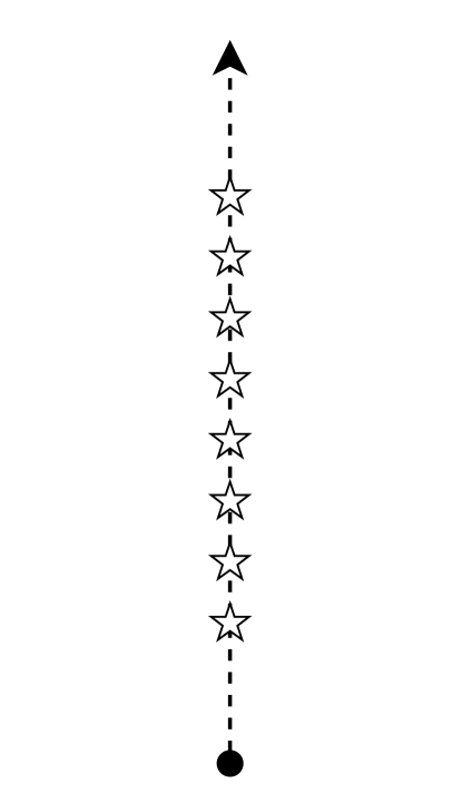
(a) Volumetric

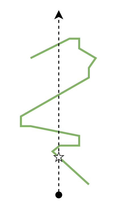
(b) Surface

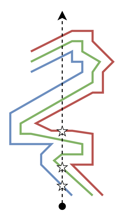
(c) Ours.

Figure 2: Different sampling strategies: a) volumetric rendering’s dense sampling; b) single sampling point, as in surface rendering; c) our method, only sampling the first intersection with each surface.

DoNeRF reduces sample count by only sampling around depth values predicted by a separate MLP, which, however, requires access to ground-truth depth maps [27]. AdaNeRF explicitly introduces sampling sparsity during the course of training [18]. HybridNeRF introduces a hybrid surface–volume representation that encourages surfaces over volumetric rendering [42]. AdaptiveShells restrict sampling to a small shell around the surface [47]. This shell is represented by a triangle mesh, which is rasterized to find the sampling range. Similar to them, we also use triangle rasterization to find sampling locations. However, our method finds all sampling locations via rasterization, while AdaptiveShells still employs standard volume rendering within the surface envelope. Consequently, AdaptiveShells still represents the scene with a 3D volume texture, while our multi-layer formulation enables the usage of 2D textures. Our method also differs in how we obtain the surface envelope. While AdaptiveShells learns a single SDF and determines the width of the envelope with a spatially-varying kernel, we progressively learn multiple, separate SDFs.

NRDF employs a two-layered mesh [44]. Both the outer and inner mesh are rasterized and feature vectors are read from the surfaces, which are decoded by a convolutional neural network (CNN). In turn, our textures directly store view-dependent opacities and colors and we do not require a CNN decoder. Further, NRDF heuristically extracts the two layers via marching cubes with different density thresholds, while we propose a progressive multi-SDF training strategy for obtaining layered meshes. Similar to us, QuadFields also aggregate opacities and view-dependent colors from multiple ray-triangle intersections [38]. However, they require blending in depth order, necessitating ray casting or depth peeling, whereas our formulation allows us to simply blend layers in a fixed order. Simultaneously, our meshes are significantly more compact than theirs.

Another line of work aims for a single sample per ray. MobileNeRF represents the scene with a coarse proxy mesh equipped with a binary opacity mask to increase expressivity [5]. BakedSDF [51], NeRF2Mesh [41], NeRFMeshing [31] and BOG[34] first perform a 3D reconstruction of the scene, convert their respective training-time representation into a mesh, and then fit an appearance model to the mesh. While these single-surface approaches are fastest, they struggle with reconstructing fuzzy geometries. Even if it would be possible to accurately reconstruct fuzzy geometry from multi-view data, representing individual hairs with hard geometry requires a lot of memory [2].

2.2 3D Reconstruction

Earlier methods for 3D reconstruction were often based on image matching [10, 37]. More recent works directly fit level-set representations via differentiable rendering [28, 49, 29, 43]. To improve convergence, many approaches convert an SDF to a volumetric density on-the-fly, which is then used for standard volume rendering [50, 45, 46, 54, 35, 19]. A number of recent methods also show that depth maps rendered from 2D or 3D Gaussians can be converted into a high-quality surface representation via volumetric fusion [15, 7, 55, 56].

3 Preliminaries

In this section we provide a brief introduction to volume- and surface-based representations and related notations.

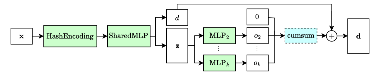
Figure 3: Our $k$-SDF network, predicting $k$ distance values as described in Section 4.1.

Rendering equation: A ray $\mathbf{r}$ in 3D space is parameterized by its origin $\mathbf{o}\in\mathbb{R}^{3}$ and unit direction $\mathbf{v}\in\mathbb{S}^{2}$. A 3D point at distance $t$ along ray $r$ is given by $\mathbf{r}(t)=\mathbf{o}+\mathbf{v}t$. Let $\sigma$ denote a density field, which assigns a nonnegative density value $\sigma(\mathbf{x})\in\mathbb{R}_{+}$ to each 3D point $\mathbf{x}\in\mathbb{R}^{3}$, and let $\xi$ be a vector field providing an RGB color $\xi(\mathbf{x},\mathbf{v})$ for each point $\mathbf{x}\in\mathbb{R}^{3}$ and direction $\mathbf{v}\in\mathbb{S}^{2}$. We can render $\xi$ along ray $r$ for a given density field $\sigma$ using the following equation [24]:

$$\mathcal{R}(\mathbf{r}\mid\sigma,\xi)=\int_{0}^{\infty}\sigma(\mathbf{r}(t))\,\xi(\mathbf{r}(t),\mathbf{v})\,w_{\text{r}}(t)\,dt\,\text{,}$$ (1)

where $w_{\text{r}}(t)=\exp\!\left[-\int_{0}^{t}\sigma(\mathbf{r}(s))\,ds\right]$.

Volume-based representations (NeRF): NeRF models a scene as a volume – with absorption and emission but without scattering effects [39] – parametrized as $(\sigma,\xi)$. NeRF numerically approximates Equation 1 with quadrature [22], densely sampling rays to render each pixel, as illustrated in Figure 2(a).

Surface-based representations (NeuS): Many surface-based representations have been proposed [49, 23, 50]; our work is built upon NeuS [45], as its densities weighting function – for which we refer to the original paper – is unbiased and occlusion-aware. In short, NeuS represents a surface implicitly by modeling it through a neural SDF, trained with differentiable volumetric rendering. A logistic distribution function $\phi_{\beta}$ maps distance values $d$ to densities as follows:

$$\phi_{\beta}(d)=\beta e^{-\beta d}/\left(1+e^{-\beta d}\right)^{2}\,.$$ (2)

Here, the spread of densities around the surface (zero-level set) is controlled by the scalar $\beta$. A small $\beta$ results in fuzzy densities, while in the limit $\beta\rightarrow\infty$ densities are sharp, impulse functions for points on the implicit surface. While NeuS regards $\beta$ as a learnable parameter, [35] showed how controlling it explicitly leads to better reconstructions. In our case, scheduling $\beta$ ensures that densities shift from being widely spread to being peaked by the end of the training. When densities are peaked, the representation can be baked into a mesh suitable for efficient rendering. However, in this case, all appearance information is condensed on a single point (Figure 2(b)); therefore, surface-based methods are not able to model semi-transparent surfaces, strongly limiting their ability to handle mixed pixels often representing thin structures, which are notoriously missed [51].

4 Method

In this section, we describe our proposed representation, Volumetric Surfaces, in detail. We begin with its implicit geometry definition, then cover rendering, training, and baking. We also discuss and justify our design choices.

4.1 $k$-SDF

Our new representation, called $k$-SDF, models $k$ surfaces as distinct signed distance fields $\{d_{1},\ldots,d_{k}\}$. To composite the surfaces, $k$-SDF is endowed with an additional transparency field $\alpha$, which assigns a view-dependent transparency value $\alpha(\mathbf{x},\mathbf{v})\in[0,1]$ to each 3D point $\mathbf{x}$. The transparency field enables modeling semi-transparent surfaces. Additionally, we have a color field $\xi$ to render images. Given a ray $\mathbf{r}$, we can render a $k$-SDF $(d_{1:k},\alpha,\xi)$ using the following rendering equation that generalizes Equation 1:

$$\mathcal{R}_{\beta}(\mathbf{r}\mid d_{1:k},\alpha,\xi)=\sum_{i=1}^{k}\mathcal{R}_{\beta}(\mathbf{r}\mid d_{i},\xi)\mathcal{R}_{\beta}(\mathbf{r}\mid d_{i},\alpha)w_{i}\text{,}$$ (3)

where $w_{i}=\prod_{j=1}^{i}\mathcal{(}1-\mathcal{R}_{\beta}(\mathbf{r}\mid d_{j},\alpha))$ and, for the sake of compactness, $\mathcal{R}_{\beta}(\mathbf{r}\mid d_{i},\gamma)$ stands for $\mathcal{R}(\mathbf{r}\mid\phi_{\beta}\circ d_{i},\gamma)$. Similarly to other SDF-based representations [45], our per-surface density field is derived from the signed distance field $d_{i}$ via a parametrized logistic function (Equation 2).

Support surfaces as shells: Blending weights in Equation 3 are order-dependent, but we cannot guarantee that lower-ranked densities are positioned closer to the camera. To avoid sorting, we model our set of surfaces as shells. This ensures that layers are traversed in ray-intersection order. We model our $k$-SDF with a main surface represented as an SDF $d$, and a set of $k-1$ support surfaces represented as offset fields $\{o_{2},\ldots,o_{k}\}$ (Figure 4) from $d$’s zero-level set. The signed distance functions for each surface are thus given by:

$$d_{1:k} =(d,d+o_{2},\ldots,d+o_{k})\,\text{.}$$ (4)

A surface defined by a positive offset is contained inside the main one, while a negative offset yields a surface containing the main one. We force the sign of a predicted offset using a softplus activation function multiplied by the desired sign. To model more than two support surfaces, while enforcing the order property, we run a cumulative sum (separately on negative and positive offsets) and use resulting displacements to parameterize the support surfaces. Figure 3 illustrates a simplified version of our model, where all offsets are positive.

Rendering individual surfaces: We sample $n$ points $\{\mathbf{x}_{1},\ldots,\mathbf{x}_{n}\}$ for each ray $\mathbf{r}$. RGB and transparency fields ($\xi$, $\alpha$) are conditioned on the encoded sample positions $\psi(\mathbf{x}_{i})$, view direction $\mathbf{v}$, the per-sample, per-surface SDF normal $\mathbf{n}_{i,j}$ and a geometric feature vector $\mathbf{z}_{i}$ predicted by the shared MLP decoder of the $k$-SDF net. The rendered color $\mathcal{C}_{j}(\mathbf{r})$ and transparency $\mathcal{A}_{j}(\mathbf{r})$ for each surface $j$ and ray $\mathbf{r}$ are then given by:

$$\mathcal{C}_{j}(\mathbf{r}) =\sum_{i=1}^{n}w_{i,j}\xi(\psi(\mathbf{x}_{i}),\mathbf{v},\mathbf{n}_{i,j},\mathbf{z}_{i})\text{,}$$ (5)

$$\mathcal{A}_{j}(\mathbf{r}) =\sum_{i=1}^{n}w_{i,j}\alpha(\psi(\mathbf{x}_{i}),\mathbf{v},\mathbf{n}_{i,j},\mathbf{z}_{i})\text{.}$$ (6)

Figure 4: $3$-SDF example visualization (signed distance and $\beta$-controlled integration weights). a) Initialization of the support surfaces as constant displacements from the main SDF. b) Densities peaked at the end of training. The two support surfaces are displace by trained offsets $(o_{1},o_{2})$, $d$: $\mathcolor{surfblue}{d_{1}}=\mathcolor{surfgreen}{d}-o_{1}$, $\mathcolor{surfred}{d_{2}}=\mathcolor{surfgreen}{d}+o_{2}$.

4.2 Surface Blending

We now rewrite Equation 3 as a fixed-order alpha blending of the rendered surface color and transparency:

$$\mathcal{R}(\mathbf{r})=\sum_{i=1}^{k}\mathcal{C}_{i}(\mathbf{r})\mathcal{A}_{i}(\mathbf{r})w_{i}\text{,}$$ (7)

where $w_{i}=\prod_{j=1}^{i}\left(1-\mathcal{A}_{j}(\mathbf{r})\right)$.

Transparency Attenuation: Blending different hard surfaces might result in clear cut-offs at their borders, especially noticeable from test views. We prefer smoother transitions towards full transparency. We achieve this by multiplying predicted transparencies with a weight $\alpha_{\text{w}}$ that depends on the angle between the view direction and the surface normal, downweighting the contribution from grazing angles. Specifically, we use

$$\alpha_{\text{w}}=2\cdot\text{Sigmoid}(10\cdot|\mathbf{v}\cdot\mathbf{n}|)-1\text{.}$$ (8)

4.3 Training and Baking

Our method is composed of two main stages. First, we optimize an implicit representation of $k$ surfaces and their appearances. Then, we fine-tune resolution-bounded neural textures over their explicit (meshes) representation. In the following, we describe both phases in detail.

4.4 Implicit Surfaces

We first train a standard NeuS-like [45] model for 100,000 iterations, during which $\beta$ is scheduled to go from large $\phi_{\beta_{1}}$ to thin densities $\phi_{\beta_{2}}$ exponentially. In practice, we find that training the $k$-SDF model from scratch with predicted transparencies leads to the presence of fully transparent geometry in the reconstruction, which we want to avoid. The reconstructed main surface acts as an anchor for the initialization of the remaining $k-1$ support surfaces, represented as shells from the main surface uniformly distanced by $\Delta o$. The mathematical formulation of $k$-SDF (Section 4.1) allows us to initialize support surfaces on the inside and on the outside of the main SDF; however, we observed that initializing them all on the inside leads to more stable runs. This is because the reconstructed main surface tends to be conservative, acting as an outer shell of the scene content. In practice, this leads support surfaces to be initialized on the outside to be modeled as fully transparent in the very first iterations of joint training. As transparent surfaces do not contribute to the final image, gradient flow is inhibited and the unused support surfaces do not recover. While we have observed the optimization to be robust under different values of $\Delta o$, we found a good balance by setting it by the logistic distribution function $\phi_{\beta}$ standard deviation $(1/\beta)\pi/\sqrt{3}$. The full model, composed of all surfaces, is trained for 50,000 iterations starting from $\phi_{\beta_{2}}$, until a $\phi_{\beta_{3}}$ value for which all surfaces are modeled as peaked densities. When this happens, our rendering process collapses to a simple blending of hard surfaces (Figure 2(c)), making the reconstructed set of implicit surfaces optimal for the later steps.

During training, we enforce two additional losses on all surfaces. The Eikonal loss [13], calculated on points in the vicinity of the zero-level sets and on randomly sampled points, and a curvature loss [35] on near-surfaces points, to push the optimization toward smooth solutions. We minimize $\mathcal{L}=\mathcal{L}_{\text{c}}+\lambda_{\text{e}}\mathcal{L}_{\text{e}}+\lambda_{\text{s}}\mathcal{L}_{\text{s}}$, where $\mathcal{L}_{\text{c}}$ is the standard $l_{1}$ pixel-wise color loss, $\mathcal{L}_{\text{e}}$ is the Eikonal loss, and $\mathcal{L}_{\text{s}}$ is the curvature term. We use weights $\lambda_{\text{e}}=0.04$ and $\lambda_{\text{s}}=0.65$.

Occupancy grid: As training progresses and densities peak, our volumetric rendering samples are gradually positioned closer to the zero-level sets of the signed distance functions, since points farther away would be in empty space. To do so, we compute per-surface binary occupancy values by describing as occupied voxels those whose center point’s $\left|d\right|$ value, together with the current $\beta$ and the voxel’s space diagonal, would allow any point in the voxel volume to have density above a $10^{-4}$ threshold. Per-surface occupancy values are then aggregated with an or operation, resulting in a single binary occupancy grid. Rays traverse the grid to sample $n$ points uniformly in occupied space. In our experiments, we used a grid of resolution $256^{3}$.

Importance sampling: We adopt hierarchical sampling from NeuS [45], extending it to the $k$-surfaces case. Starting from the $n$ uniform samples, each SDF is evaluated to compute $k$ CDFs; these are summed together and normalized. The resulting probability distribution is used to sample $m/2$ additional points that are added to the previous $n$. The whole operation is then repeated on the expanded set of points to add $m/2$ more samples. The resulting number of samples per ray is then $n+m$. The kernel size $\beta$ used to compute weights at the second iteration is the same as used during rendering, $\beta$ at the second iteration is half the value.

Mesh baking: We extract $k$-SDF zero-level sets as high-resolution meshes using marching cubes [21]. and heavily simplify them [12] to 0.02% of the original number of triangles (approximately 2 MB each for synthetic scenes), meeting the strict computing and memory requirements of mobile hardware. Finally, we compute UV atlases for these lightweight meshes with xatlas [52]. This is a fundamental step for the next stage, in which we train per-mesh neural SH textures, which are later baked as explicit textures.

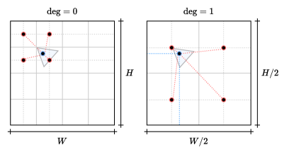
Figure 5: Bilinear interpolation in our mixed-resolution textures. Instead of directly querying the blue 2D point, we predict the values of its surrounding texel centers (red points) and bilinearly interpolate them. This makes the neural texture texture-dependent, with predefined width $W$ and height $H$.

Table 1: Results are averaged across all testing scenes. Highlighted baselines meet the compute and/or memory requirements to run on general-purpose hardware (via WebGL) without modifications, as discussed in Section 2.1. Methods marked with a “$\star$” show results from original papers, as code is unavailable. MobileNeRF and Instant-NGP results on Shelly from AdaptiveShells. DTU is evaluated on masked foreground. PermutoSDF trained until densities are fully peaked ($\phi_{\beta_{3}})$. Metrics not provided by a baseline are denoted with “—”. Please note that the Shelly dataset, as released by the authors, has a large overlap of views between test and training sets. All our experiments were conducted on a cleaned version of the dataset, free of this problem. However, a fair comparison with baselines whose code is not public remains difficult. Our per-scene metrics are reported in the supplementary material.

	Shelly [47]			Custom (ours + [38])			DTU [16] (scans 83, 105)
Method	PSNR $\uparrow$	SSIM $\uparrow$	LPIPS $\downarrow$	PSNR $\uparrow$	SSIM $\uparrow$	LPIPS $\downarrow$	PSNR $\uparrow$	SSIM $\uparrow$	LPIPS $\downarrow$
3DGS [17]	35.443	0.964	0.064	37.345	0.982	0.147	38.060	0.989	0.086
Instant-NGP [26]	33.220	0.922	0.125	31.133	0.935	0.132	38.245	—	—
PermutoSDF [35]	29.850	0.950	0.129	33.306	0.961	0.193	36.312	0.988	0.098
AdaptiveShells⋆ [47]	36.020	0.954	0.079	—	—	—	—	—	—
QuadFields⋆ [38]	35.130	0.954	0.073	—	—	—	—	—	—
MobileNeRF [5]	31.620	0.911	0.129	—	—	—	—	—	—
3-Mesh	33.247	0.977	0.118	34.843	0.970	0.175	36.242	0.984	0.095
5-Mesh	34.098	0.979	0.114	35.419	0.974	0.171	36.504	0.985	0.089
7-Mesh	34.331	0.980	0.113	35.605	0.976	0.169	36.624	0.987	0.087
9-Mesh	34.220	0.981	0.113	35.716	0.978	0.167	36.826	0.986	0.086

4.5 Mesh Texturing

Lastly, we train our final per-surface appearance model based on neural textures. A neural texture is implemented as a hash-grid with input dimension 2 and a small decoder MLP with output dimension dependent on the SH degree it models. The $i$-th neural texture predicts $\overline{\mathbf{sh}_{i}}\in\mathbb{R}^{4\times c_{\text{deg}}}$, with $c=\{1,3,5,7\}$. The outputs of all neural textures are concatenated over the coefficient dimension ($\mathbf{sh}\!\in\!\mathbb{R}^{4\times(\text{deg}+1)^{2}}$) and decoded with view direction $\mathbf{v}$ to predict RGBA. Specifically, we discretize our neural textures by grounding them to a fixed target baking resolution. In this setting, each point $\mathbf{x}\!\in\!\mathbb{R}^{3}$ on the surface of a mesh is mapped to a point $\overline{\mathbf{x}}\!\in\![0,1]^{2}$ in UV space. SH coefficients at $\overline{\mathbf{x}}$ are predicted as the result of a bilinear interpolation of predictions at neighboring texels centers $\{\overline{\mathbf{x}}_{i}\}_{1,\ldots,4}$, as visualized in Figure 5. This effectively mimics how OpenGL fragment shaders access and interpolate texture values; by doing so, we optimize our texture values such that when displayed in our real-time renderer, images match – up to numerical precision – those synthesized by our differentiable renderer. This final phase is trained for 15,000 iterations without additional losses.

Mixed resolutions: Storing all textures at full resolution ($2048^{2}$) is impractical on mobile devices, as it would require approximately 0.5 GB per mesh. We propose scaling texture resolution proportionally to the spherical harmonics (SH) coefficient degree: the base color is modeled at the highest resolution ($2048^{2}$), while the highest SH degree coefficients are modeled at the lowest resolution ($256^{2}$). This approach significantly reduces the memory footprint to approximately 14 MB per mesh without compromising image quality, as shown in Table 5.

Squeezing and quantization: Neural textures predicted values $\mathbf{sh}$ are continuous and defined in an unbounded range. Before storing them, they must be squeezed to the unit range via $\hat{\mathbf{sh}}=\text{Sigmoid}(\mathbf{sh})$. Training must account for quantization to the discrete $[0,255]$ range when storing textures as images. Following MERF [33], we apply the function $q(x)=\text{round}(255x)/255$ to the predicted and squeezed coefficients. Before rendering, we re-scale value to a hyper-parameters controlled range $[v_{\text{min}},v_{\text{max}}]$:

$$\mathbf{sh}=v_{\text{min}}+(v_{\text{max}}-v_{\text{min}})q(\hat{\mathbf{sh}})$$ (9)

In practice, we observed a range of $[-15,15]$ to work well on all scenes.

Texture baking: Our resolution-grounded neural textures are easy to bake, as this only requires predicting values at texel centers and storing them. Baking results in $(\text{deg}+1)^{2}$ PNG images, where the $i$-th image stores the $i$-th coefficient of RGBA channels. The fully baked representation can finally be visualized in our WebGL renderer, which rasterizes all meshes in a fixed order and blends them in the final frame buffer before displaying the result on screen.

5 Evaluation

Our most important baselines are methods targeting real-time rendering. We identified 3DGS and MobileNeRF as our main competitors; 3DGS represents the fastest volumetric representation, while MobileNeRF is a surface-based method pioneering mobile neural graphics rendering. We compare them in terms of quality (Table 1), speed and memory footprint (Table 2). Additionally, we compare with other baselines not designed for rendering on general-purpose hardware to provide a more comprehensive overview of current methods. Aiming to represent fuzzy geometries with high quality, we focus our evaluation on object-centric datasets featuring fuzzy structures. We present results from synthetic benchmark datasets like Shelly [47], plush objects from real-world tabletop scenes (DTU [16]), and additional synthetic custom scenes (our plushy and hairy_monkey from [38]). Our method consistently achieves higher image quality than surface-based competitors and renders faster than 3DGS, even with the maximum number of surfaces. Using seven layers offers a good balance between image quality, model size, and rendering speed, as quality tends to degrade with nine meshes under the same number of training iterations. This occurs because deeper surfaces contribute less to the final pixel color than outer surfaces, leading to scaled gradient magnitudes and making them harder to optimize. Figure 6 pictures the trade-offs between frame rate and model size. While our method falls short of the latest volume-based baselines in image quality, our baked representation provides a favorable balance between quality and speed, rendering much faster on non-specialized hardware. We refer to our supplementary material for additional results visualizations.

Figure 6: Framerate vs quality comparison (laptop results from Table 2). The radius of each circle represents the memory footprint of each model as stored on disk.

Table 2: 3DGS with spherical harmonics up to degree 2, ours up to degree 3. Metrics averaged over scenes of the Shelly [47] dataset. Framerate is measured on close-up views at HD (720p) resolution on low-power laptop (Dell XPS 13 i5) (marked with $\star$) and smartphone (Samsung A52s) (marked with $\diamond$), on respective WebGL renderers (when available); memory footprint as stored on disk.

Method	FPS ${}^{\diamond}\uparrow$	FPS ${}^{\star}\uparrow$	MB $\downarrow$
3DGS [17]	8.0	18	53.6
QuadFields [38]	—	—	1213.0
Our 3-Mesh	55.0	152	43.8
Our 5-Mesh	40.0	97	69.1
Our 7-Mesh	27.5	72	97.6
Our 9-Mesh	21.5	51	133.6

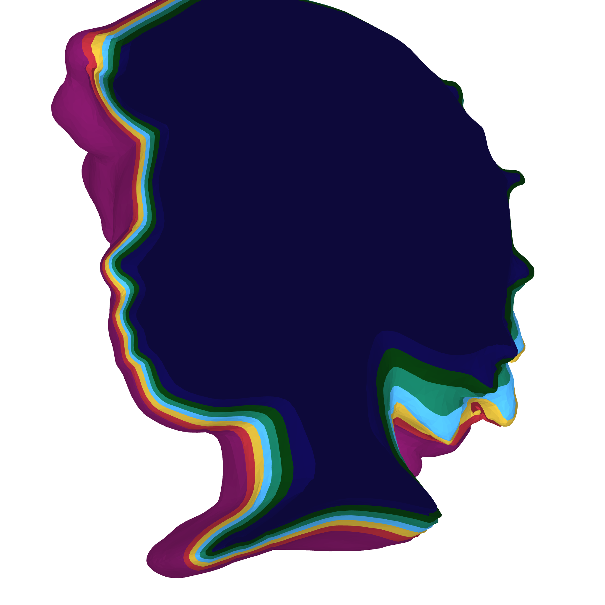
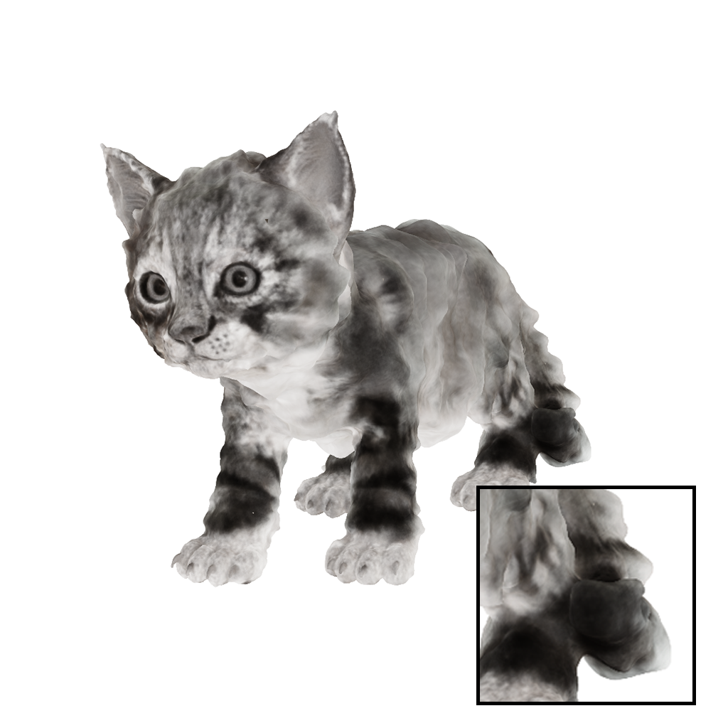
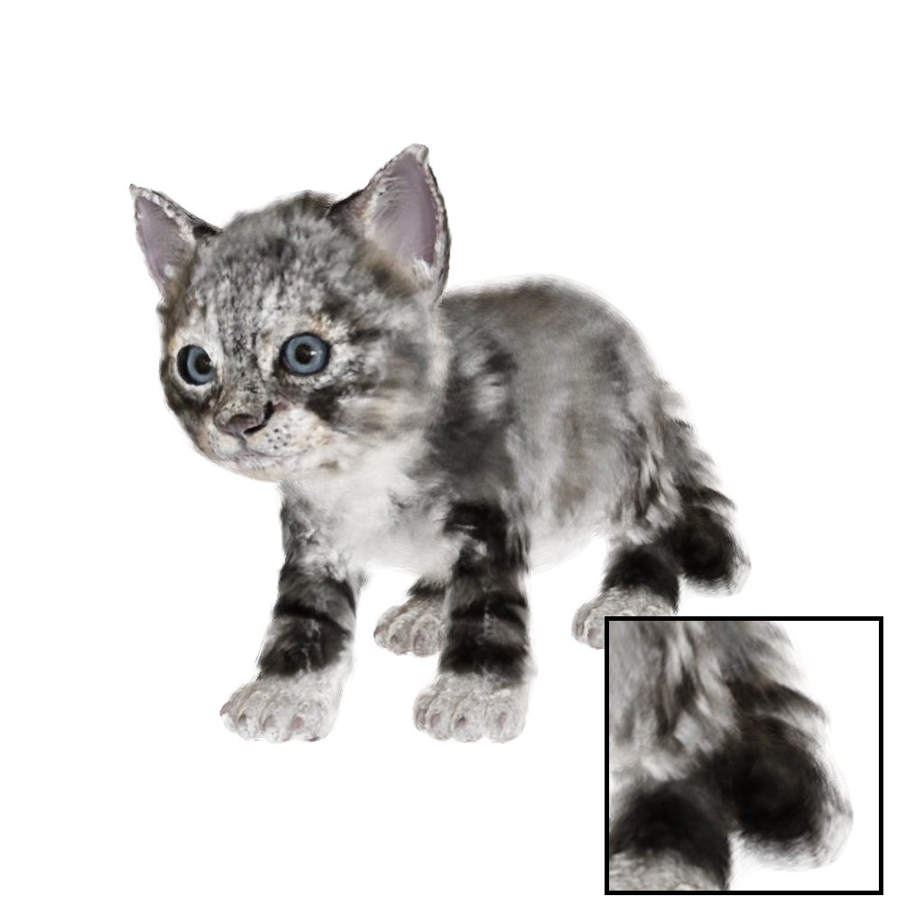
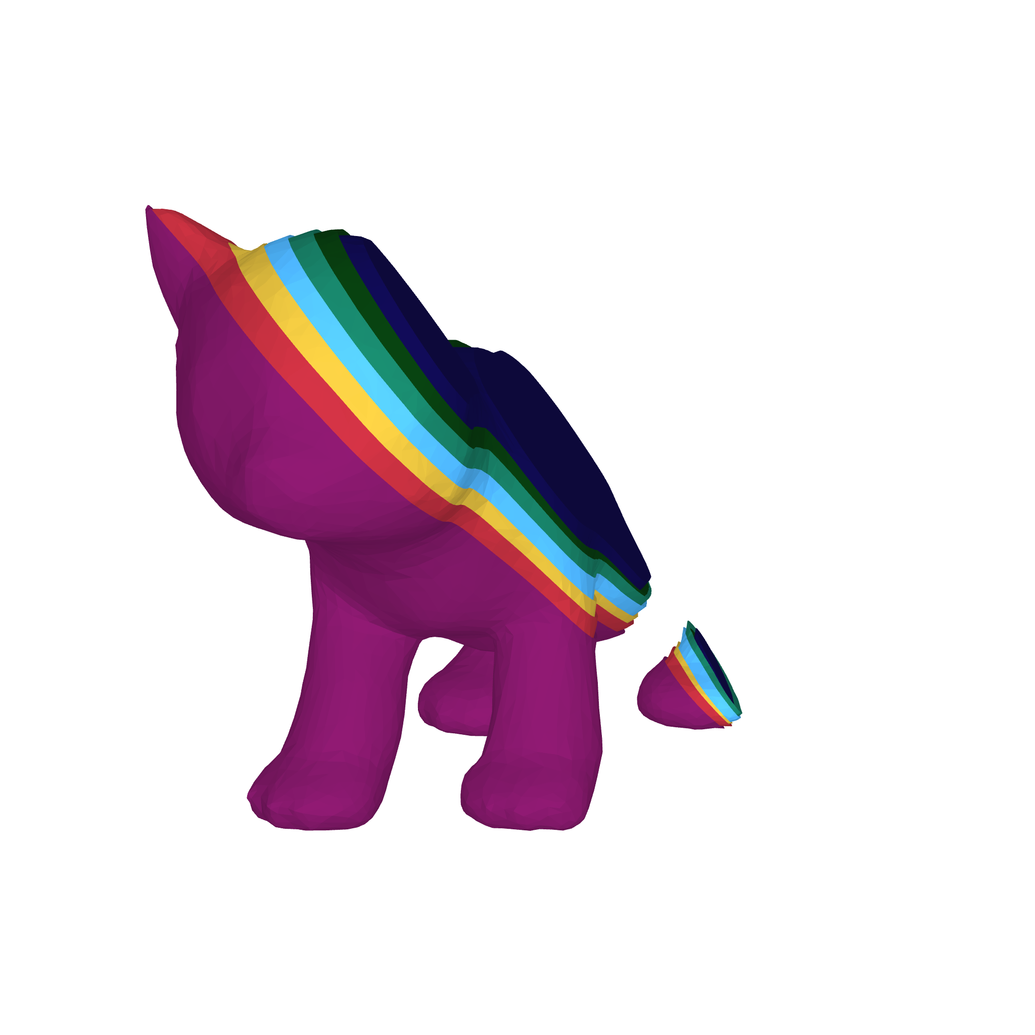
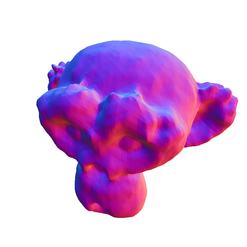
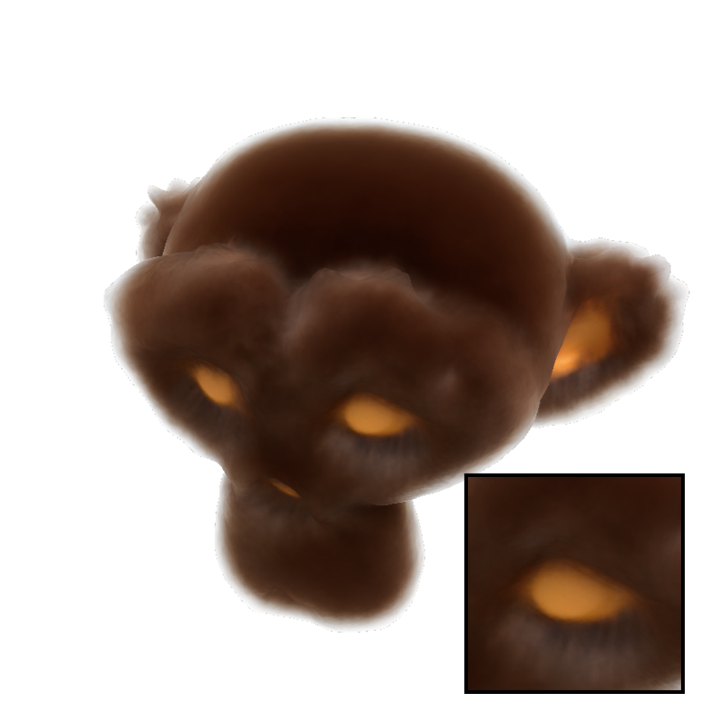
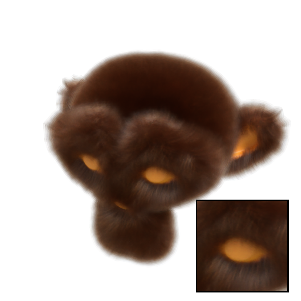
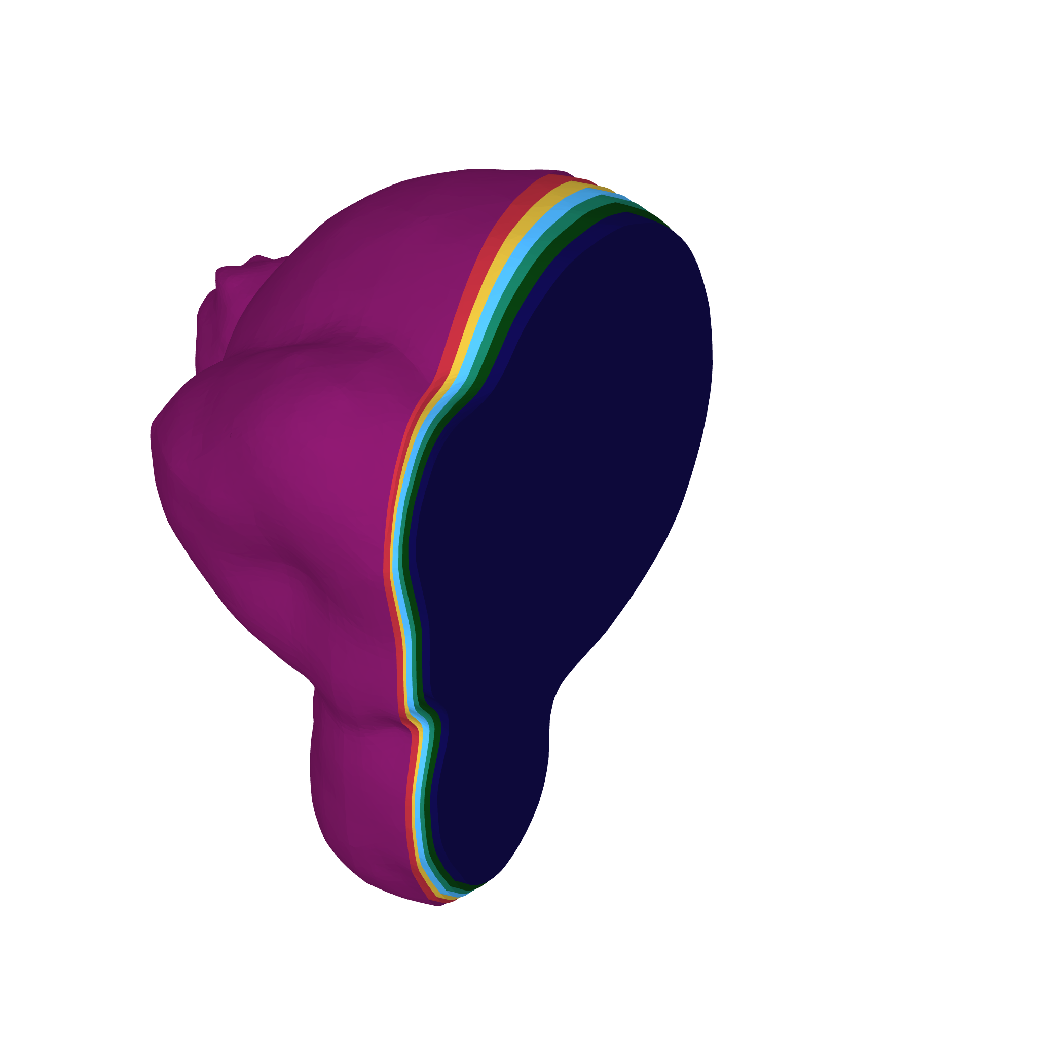
a)	b)	c)	d)

Figure 7: Qualitative comparisons between b) PermutoSDF [35], a state-of-the-art implicit surface-based method, and c) our Volumetric Surfaces demonstrate that our approach convincingly represents fuzzy objects. This is achieved by trading a) high-frequency geometry for the number of integration points, which are found by rasterizing smooth, lightweight meshes defined as d) shells around the object and traversed in a fixed order. Volumetric Surfaces enable fast rendering of fuzzy geometries on general-purpose hardware with image quality approaching the latest volumetric representations (Table 1). Scenes from Shelly [47] and QuadFields [38].

5.1 Ablations

We ablate all crucial aspects of our method and show results on both implicit (Table 3) and explicit (Table 4) geometry phases. We run our full model:

1. without view-dependent surface transparency; we observe increased model expressivity as shown by the improved image quality metrics.

2. without curvature loss during $k$-SDF training ($\lambda_{s}=0.0$), surfaces can reconstruct high-frequency details, but the image quality of the baked representation worsens. This occurs because the simplified post-baking mesh poorly aligns with the implicit one. Conversely, enabling curvature loss results in $k$-SDF reconstructing smoother surfaces with meshes that closely align with their implicit counterparts, maintaining a low triangle cost. Additionally, this demonstrates how our high-capacity appearance modeling compensates for missing geometric details.

3. without transparency attenuation (Section 4.2) at grazing angles (no $\alpha_{w}$). We observe how it significantly reduces rendering errors, particularly at object boundaries.

4. with constant support surface offsets ($\Delta o$), which are not trained and remain fixed at their initial values. We observe how results worsen significantly. Training offsets allows spacing to adapt optimally to each scene.

Visualizations of the ablations are provided in our supplementary material.

Table 3: Ablation results on $5$-SDF averaged over Shelly dataset scenes [47]. See Section 5.1 for explanations.

Ablation	PSNR $\uparrow$	SSIM $\uparrow$	LPIPS $\downarrow$
5-SDF, full	32.046	0.964	0.130
1) w/o view-dep. $\alpha$	31.753	0.962	0.131
2) w/o curvature $\mathcal{L}_{\text{s}}$	33.016	0.971	0.117
3) w/o $\alpha_{\text{w}}$	32.106	0.966	0.130

Table 4: Ablation results on $5$-Mesh (baked, real-time rendering assets) averaged over Shelly dataset scenes [47]. See Section 5.1.

Ablation	PSNR $\uparrow$	SSIM $\uparrow$	LPIPS $\downarrow$
5-Mesh, full	34.098	0.979	0.114
1) w/o view-dep. $\alpha$	32.713	0.975	0.120
2) w/o curvature $\mathcal{L}_{\text{s}}$	33.412	0.980	0.110
3) w/o $\alpha_{\text{w}}$	33.963	0.980	0.113
4) w. const. $\Delta o$	30.092	0.950	0.129

Table 5: Results on the khady scene from Shelly [47]. Sweep over the number of meshes and target neural textures resolution. Mixed resolutions are described in Section 4.5. Increasing neural texture resolution improves reconstruction quality up to $1024^{2}$, but performance declines beyond that. Modeling all textures at maximum resolution ($2048^{2}$) is counterproductive, as results show that a mixed-resolution approach is better in terms of image quality and memory footprint.

	PSNR $\uparrow$
Method	mixed	20482	10242	5122	2562
5-Mesh	29.82	29.82	29.85	29.76	29.48
7-Mesh	29.91	29.91	29.95	29.87	29.58
9-Mesh	29.93	29.90	29.94	28.87	29.59

5.2 Limitations

Experiments on the NeRF-Synthetic [25] dataset, which lacks fuzzy geometries, show only marginal improvements over PermutoSDF. This is likely due to increased view-dependency capacity, which tends to overfit training views and reduce test view quality. Similarly, our model excels in densely observed scenes but underperforms when training views are sparse, as our representation sacrifices multi-view consistent geometric complexity for view-dependent effects that do not generalize well to test views.” A solution explored in [44] involves initially training a robust model (e.g., NeRF-like) and then distilling its reconstruction by using renders from randomly generated cameras as the training set for our method. The handling of thin structures remains challenging due to the underlying SDF geometry representation.

6 Conclusion

We presented Volumetric Surfaces, a multi-layer mesh representation for real-time view synthesis of fuzzy objects on a wide range of devices. Our method renders faster than state-of-the-art volume-based approaches, while being significantly more capable at reproducing fuzzy objects than single-surface methods. In future work, we would like to develop a single-stage, end-to-end training procedure that directly produces real-time renderable assets.

Acknowledgments: Plushy blender object by kaizentutorials. S.Esposito acknowledges travel support from the European Union’s Horizon 2020 research and innovation program under ELISE Grant Agreement No 951847.

Supplementary Material

7 Supplementary

In this supplementary material, we present additional visualizations (Section 7.1 and Section 7.2), comprehensive per-scene results (Section 7.3), and a deeper analysis of performance on fully solid geometries (Section 7.4).

7.1 Transparency Attenuation

We introduced transparency attenuation in Section 4.2 to reduce visual artifacts at object boundaries. Figure 8, cropped from our ablation experiments, highlights its significance in our method.

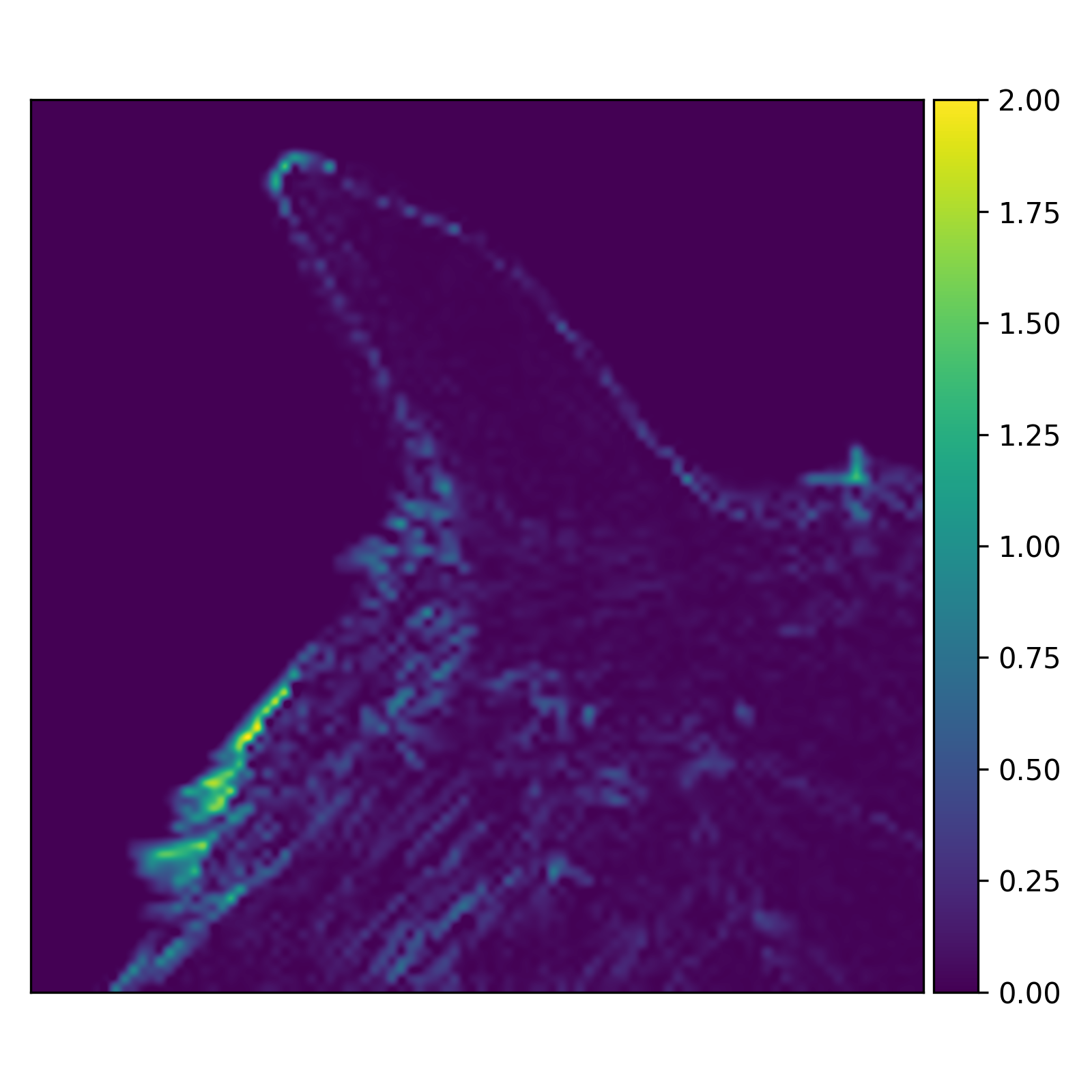
$a$) without $\alpha_{\text{w}}$	$b$) with $\alpha_{\text{w}}$

Figure 8: Rendering error crop without (a) and with (b) transparency-decay, resulting in a 2.13 dB PSNR gain. Scene from the Shelly dataset [47].

7.2 Additional Visualizations

We provide additional qualitative comparisons on our evaluation scenes of the DTU [16] dataset. Additionally, we provide visualizations of per-surface rendering before alpha blending (Figure 10 and Figure 11) to illustrate how each layer, based on its position and opacity, contributes with its view-dependent appearance model to the final image.

7.3 Per-scene Results

Table 6, Table 8 and Table 8 present the per-scene values that are averaged in Table 1.

7.4 Fully Solid Scenes

Although not our targeted use case, we tested our method on the fully solid scenes of the NeRF-Synthetic dataset [25] (which does not contain any fuzzy objects). In these scenes, our method outperforms PermutoSDF [35] but lags behind other baselines, as mentioned in Section 5.2. We approach fuzzy surface modeling not by emphasizing intricate geometric details but by increasing the number of samples with optimized spatial distribution, as these factors are crucial for the accurate representation of such effects. Therefore, our method promotes smoother surfaces, leading to smoothed angles and overly simplified geometry in under-observed areas (Figure 13). Fully solid scenes could be optimally modeled as a single surface. However, SDF-based methods struggle in handling thin structures, with the optimization failing to extract them reliability (BakedSDF [51], BOG[34]). Our surfaces smoothing, combined with view-dependent transparency, results in thin structures being reconstructed as view-dependent effects (Figure 12). Consequently, our model tends to overfit training views, yielding a larger gap between training and test views quality (Table 9).

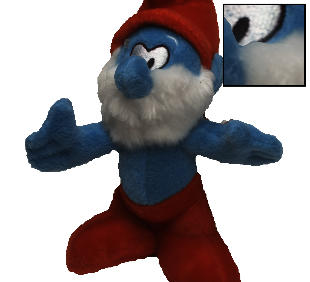
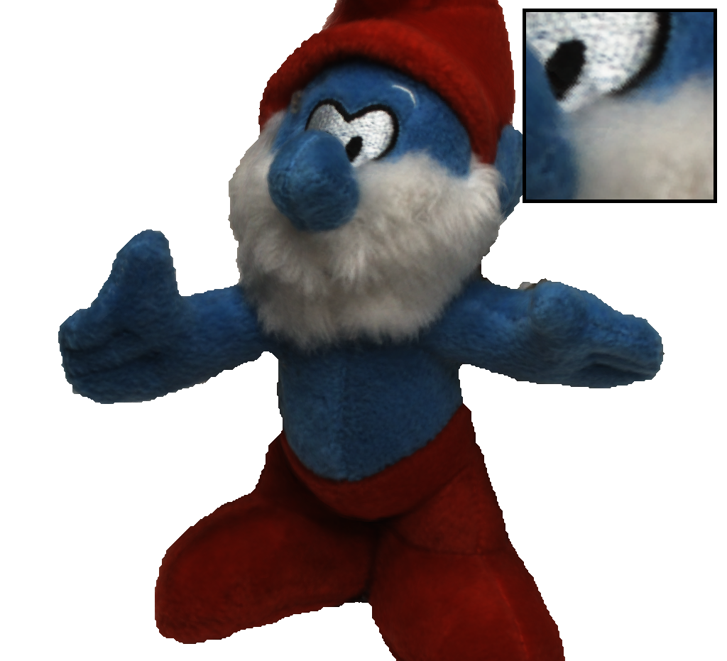
PermutoSDF [35]	7-Mesh (ours)
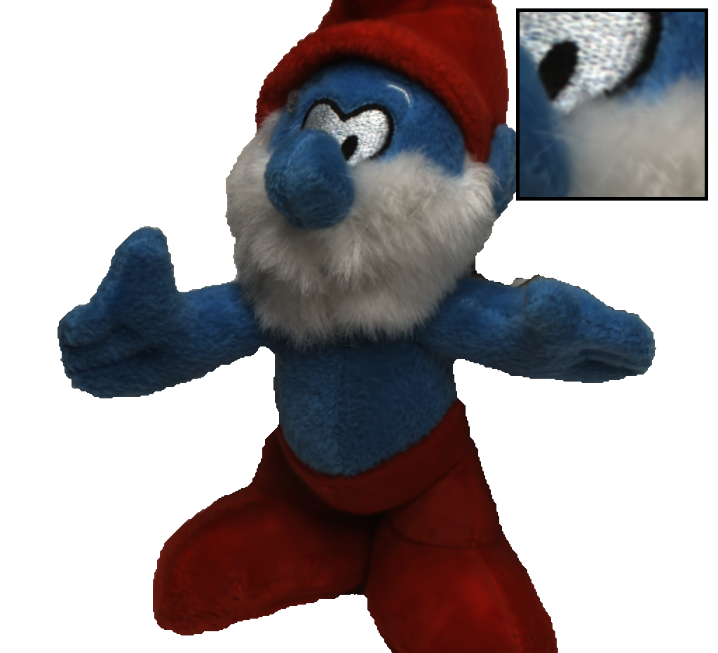
3DGS [17]	Ground truth
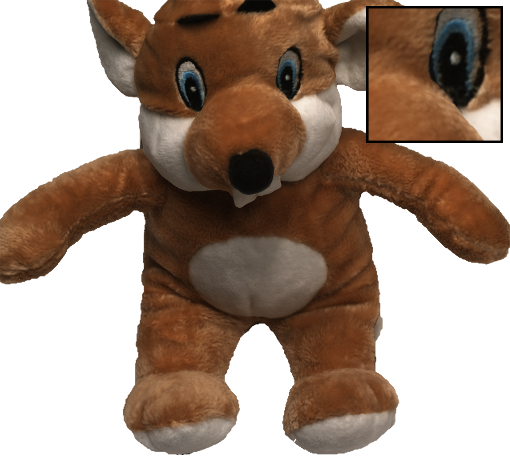
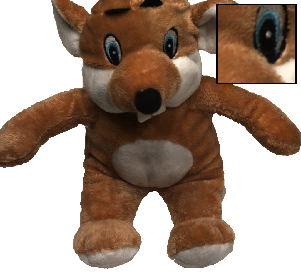
PermutoSDF [35]	7-Mesh (ours)
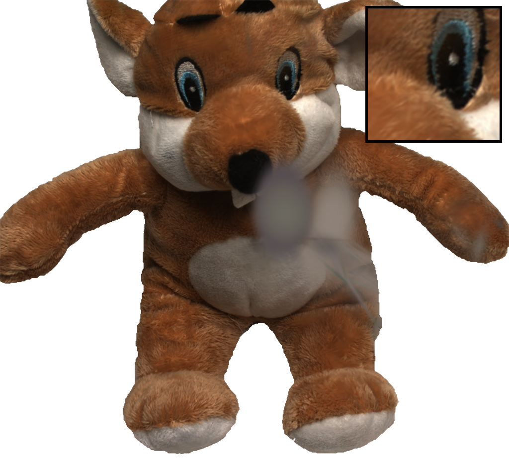
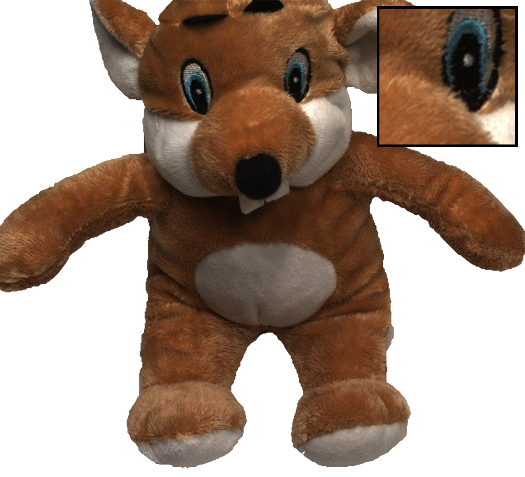
3DGS [17]	Ground truth

Figure 9: Scenes from the DTU dataset [16].

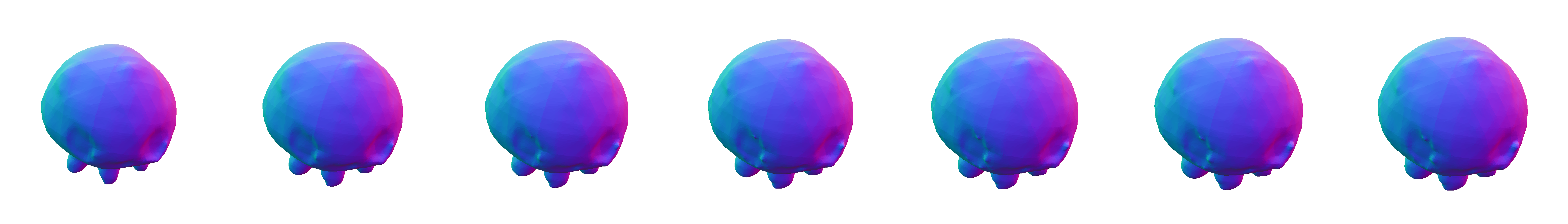
a) Surface normals.

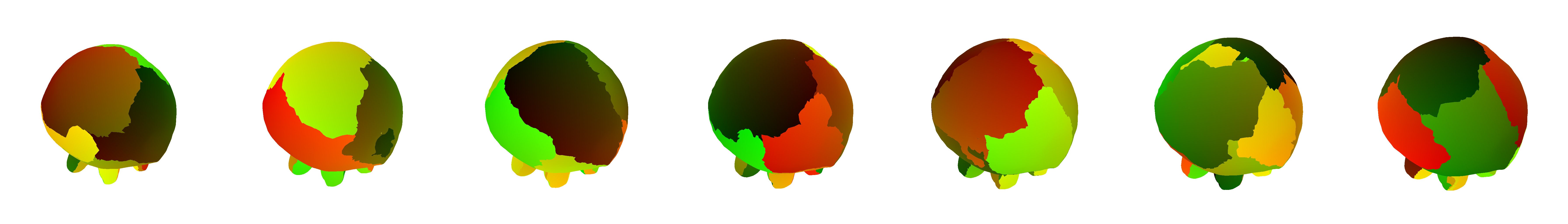
b) Surface UVs.

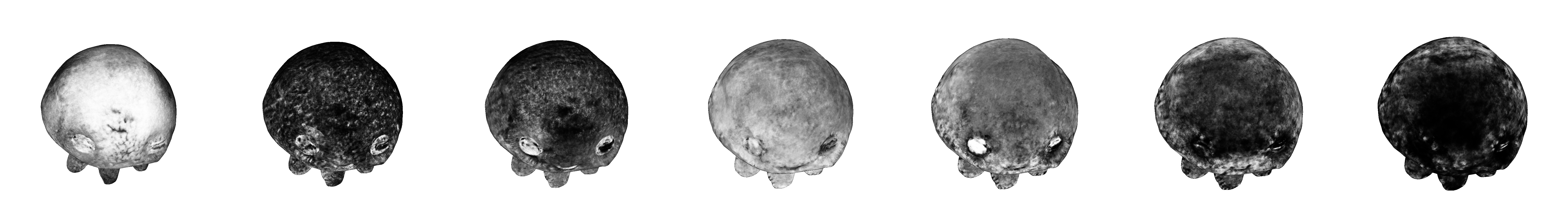
c) Surface opacity.

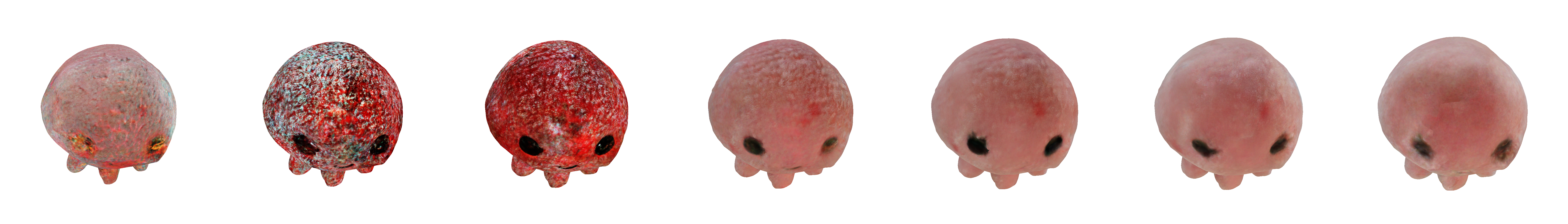
d) Surface colors (RGB).

Figure 10: 7-Meshes render buffers. Layers order: left to right is inner to outer. Individual layer colors and alpha buffers are blended as described in Section 4.2.

a) Surface normals.

b) Surface UVs.

c) Surface opacity.

d) Surface colors (RGB).

Figure 11: 7-Meshes render buffers. Layers order: left to right is inner to outer. Individual layer color and alpha buffers are blended as described in Section 4.2.

Table 6: Per-scene results for baselines.

		PermutoSDF [35]			3DGS [17]
Dataset	Scene	PSNR $\uparrow$	SSIM $\uparrow$	LPIPS $\downarrow$	PSNR $\uparrow$	SSIM $\uparrow$	LPIPS $\downarrow$
Shelly [47]	fernvase	28.424	0.953	0.078	34.821	0.986	0.040
	horse	34.677	0.993	0.040	41.451	0.997	0.038
	khady	26.219	0.879	0.226	30.545	0.924	0.187
	kitten	30.913	0.971	0.093	38.169	0.991	0.050
	pug	29.480	0.953	0.168	35.959	0.983	0.089
	woolly	29.387	0.949	0.167	31.710	0.969	0.130
Custom (ours + [38])	hairy_monkey	33.672	0.977	0.194	37.672	0.990	0.142
	plushy	32.940	0.945	0.192	37.018	0.975	0.153
DTU [16] (scans 83, 105)	dtu_scan105	34.783	0.985	0.124	35.505	0.984	0.102
	dtu_scan83	37.842	0.991	0.072	40.615	0.994	0.070

Table 7: Our per-scene results.

		3-Mesh			5-Mesh
Dataset	Scene	PSNR $\uparrow$	SSIM $\uparrow$	LPIPS $\downarrow$	PSNR $\uparrow$	SSIM $\uparrow$	LPIPS $\downarrow$
Shelly [47]	fernvase	32.261	0.984	0.068	33.518	0.987	0.065
	horse	38.175	0.997	0.039	39.668	0.998	0.035
	khady	29.645	0.937	0.198	29.825	0.939	0.197
	kitten	35.681	0.990	0.080	36.739	0.992	0.077
	pug	33.569	0.982	0.141	34.014	0.985	0.138
	woolly	30.118	0.972	0.179	30.825	0.976	0.172
Custom (ours + [38])	hairy_monkey	35.433	0.983	0.182	35.894	0.985	0.180
	plushy	34.252	0.956	0.168	34.944	0.964	0.163
DTU [16] (scans 83, 105)	dtu_scan105	34.607	0.979	0.123	34.875	0.980	0.115
	dtu_scan83	37.878	0.989	0.066	38.132	0.990	0.063

Table 8: Our per-scene results.

		7-Mesh			9-Mesh
Dataset	Scene	PSNR $\uparrow$	SSIM $\uparrow$	LPIPS $\downarrow$	PSNR $\uparrow$	SSIM $\uparrow$	LPIPS $\downarrow$
Shelly [47]	fernvase	34.420	0.990	0.063	34.531	0.991	0.063
	horse	39.896	0.998	0.034	39.120	0.998	0.035
	khady	29.918	0.940	0.197	29.927	0.942	0.198
	kitten	37.022	0.993	0.076	36.946	0.993	0.076
	pug	33.984	0.984	0.139	33.994	0.984	0.140
	woolly	30.746	0.977	0.167	30.799	0.976	0.167
Custom (ours + [38])	hairy_monkey	36.081	0.986	0.177	36.130	0.987	0.175
	plushy	35.129	0.967	0.162	35.301	0.969	0.160
DTU [16] (scans 83, 105)	dtu_scan105	35.331	0.983	0.112	35.191	0.982	0.111
	dtu_scan83	37.918	0.991	0.062	38.461	0.990	0.062

Table 9: Results averaged across test scenes. In solid scenes, our method outperforms PermutoSDF (see Figure 12) but lags behind other baselines. We explain this behavior in Section 7.4. Methods marked with a $\star$ show results taken from original papers, as code is unavailable. MobileNeRF and Instant-NGP results on Shelly from AdaptiveShells. PermutoSDF trained until densities are fully peaked ($\phi_{\beta_{3}})$. Metrics not provided by a baseline are denoted with “—”.

	NeRF-Synthetic [25]
	Train			Test
Method	PSNR $\uparrow$	SSIM $\uparrow$	LPIPS $\downarrow$	PSNR $\uparrow$	SSIM $\uparrow$	LPIPS $\downarrow$
3DGS [17]	36.763	0.991	0.030	33.227	0.981	0.037
Instant-NGP [26]	—	—	—	33.180	—	—
PermutoSDF [35]	29.311	0.975	0.057	28.052	0.966	0.065
AdaptiveShells ⋆	—	—	—	31.840	0.957	0.056
QuadFields ⋆	—	—	—	31.000	0.952	0.069
MobileNeRF [5]	—	—	—	30.900	0.947	0.060
3-Mesh	32.255	0.982	0.061	28.366	0.957	0.085
5-Mesh	33.077	0.985	0.056	28.644	0.958	0.083
7-Mesh	33.159	0.985	0.057	28.748	0.959	0.083
9-Mesh	33.044	0.985	0.058	28.656	0.959	0.084

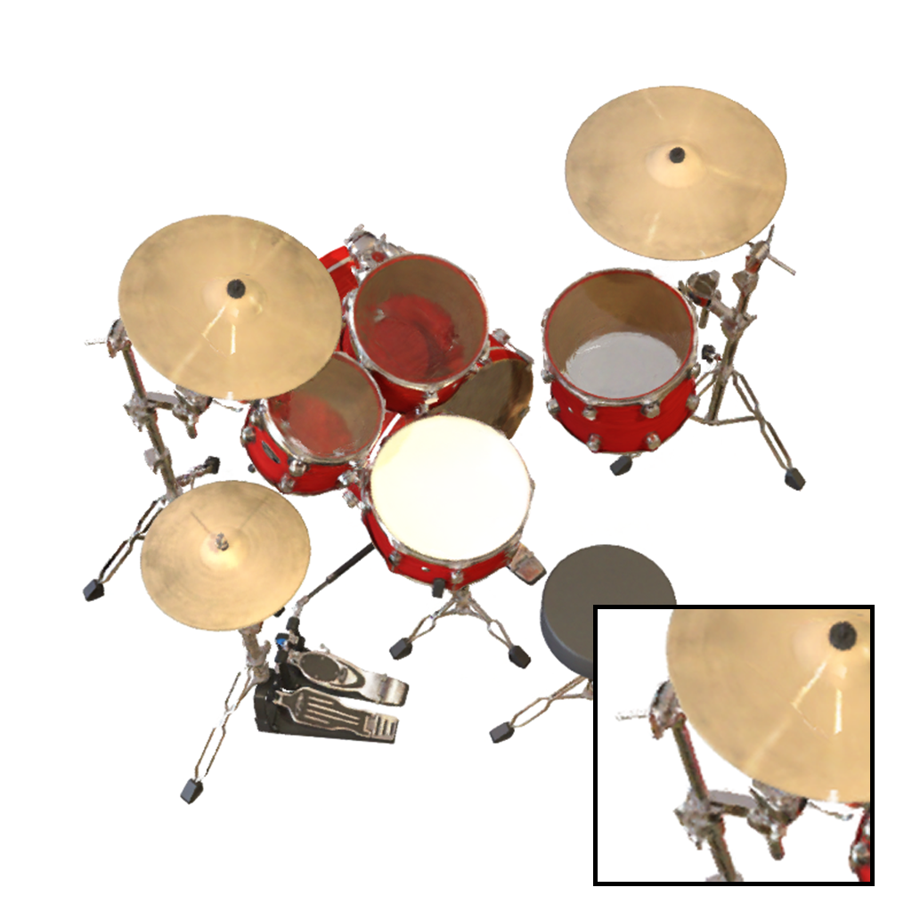
PermutoSDF [35]	7-Mesh (ours)
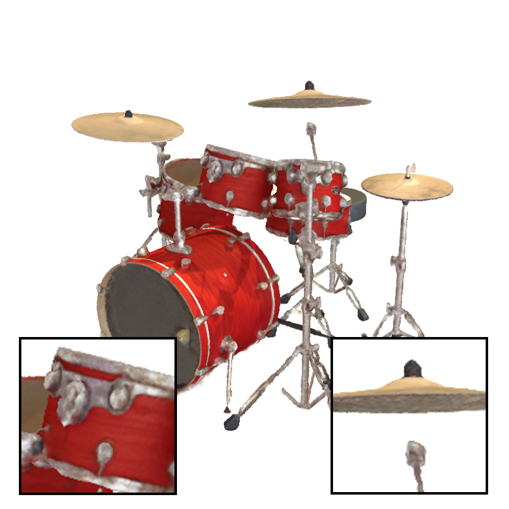
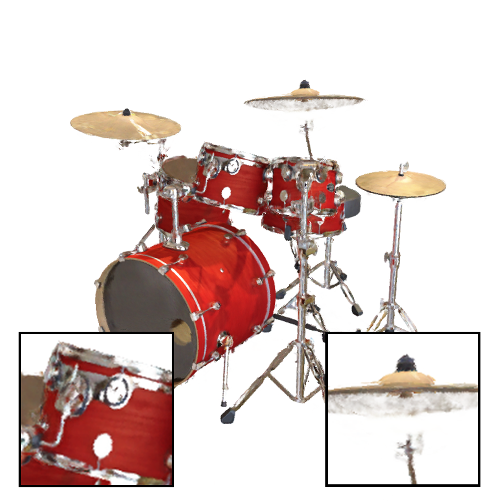
PermutoSDF [35]	7-Mesh (ours)

Figure 12: Top row: train view; bottom row: test view. Scene from NeRF-Synthetic [25].

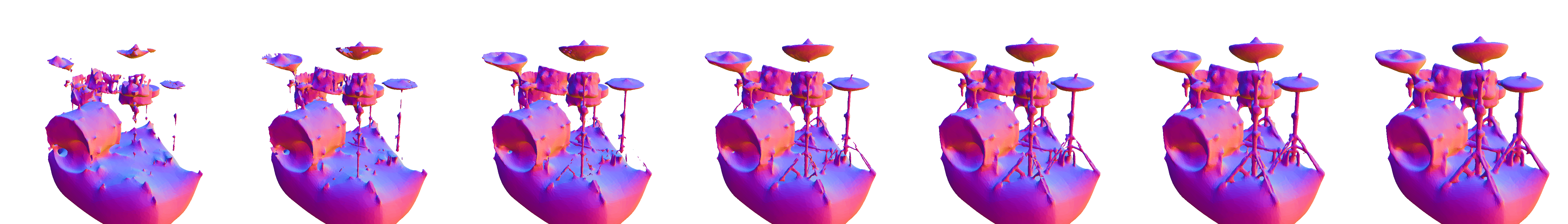
Figure 13: Surface normals. Scene from NeRF-Synthetic [25]

References

- Aliev et al. [2019] Kara-Ali Aliev, Dmitry Ulyanov, and Victor S. Lempitsky. Neural point-based graphics. arXiv.org, 1906.08240, 2019.
- Bhokare et al. [2024] Gaurav Bhokare, Eisen Montalvo, Elie Diaz, and Cem Yuksel. Real-time hair rendering with hair meshes. In ACM Trans. on Graphics, 2024.
- Chen et al. [2022] Anpei Chen, Zexiang Xu, Andreas Geiger, Jingyi Yu, and Hao Su. Tensorf: Tensorial radiance fields. In Proc. of the European Conf. on Computer Vision (ECCV), 2022.
- Chen and Zhang [2019] Zhiqin Chen and Hao Zhang. Learning implicit fields for generative shape modeling. In Proc. IEEE Conf. on Computer Vision and Pattern Recognition (CVPR), 2019.
- Chen et al. [2023a] Zhiqin Chen, Thomas Funkhouser, Peter Hedman, and Andrea Tagliasacchi. MobileNeRF: Exploiting the polygon rasterization pipeline for efficient neural field rendering on mobile architectures. In Proc. IEEE Conf. on Computer Vision and Pattern Recognition (CVPR), 2023a.
- Chen et al. [2023b] Zhang Chen, Zhong Li, Liangchen Song, Lele Chen, Jingyi Yu, Junsong Yuan, and Yi Xu. Neurbf: A neural fields representation with adaptive radial basis functions. In Proc. of the IEEE International Conf. on Computer Vision (ICCV), 2023b.
- Dai et al. [2024] Pinxuan Dai, Jiamin Xu, Wenxiang Xie, Xinguo Liu, Huamin Wang, and Weiwei Xu. High-quality surface reconstruction using gaussian surfels. In ACM Trans. on Graphics. Association for Computing Machinery, 2024.
- Duckworth et al. [2023] Daniel Duckworth, Peter Hedman, Christian Reiser, Peter Zhizhin, Jean-François Thibert, Mario Lučić, Richard Szeliski, and Jonathan T. Barron. Smerf: Streamable memory efficient radiance fields for real-time large-scene exploration. arXiv.org, 2312.07541, 2023.
- Esposito et al. [2022] Stefano Esposito, Daniele Baieri, Stefan Zellmann, André Hinkenjann, and Emanuele Rodolà. KiloNeuS: A versatile neural implicit surface representation for real-time rendering. arXiv.org, 2206.10885, 2022.
- Furukawa et al. [2010] Yasutaka Furukawa, Brian Curless, Steven M. Seitz, Richard Szeliski, and Google Inc. Towards internet-scale multiview stereo. In Proc. IEEE Conf. on Computer Vision and Pattern Recognition (CVPR), 2010.
- Garbin et al. [2021] Stephan J. Garbin, Marek Kowalski, Matthew Johnson, Jamie Shotton, and Julien Valentin. Fastnerf: High-fidelity neural rendering at 200fps. arXiv.org, 2021.
- Garland and Heckbert [1997] Michael Garland and Paul S. Heckbert. Surface simplification using quadric error metrics. In ACM Trans. on Graphics, pages 209–216, 1997.
- Gropp et al. [2020] Amos Gropp, Lior Yariv, Niv Haim, Matan Atzmon, and Yaron Lipman. Implicit geometric regularization for learning shapes. arXiv.org, 2002.10099, 2020.
- Hedman et al. [2021] Peter Hedman, Pratul P. Srinivasan, Ben Mildenhall, Jonathan T. Barron, and Paul Debevec. Baking neural radiance fields for real-time view synthesis. Proc. of the IEEE International Conf. on Computer Vision (ICCV), 2021.
- Huang et al. [2024] Binbin Huang, Zehao Yu, Anpei Chen, Andreas Geiger, and Shenghua Gao. 2d gaussian splatting for geometrically accurate radiance fields. In ACM Trans. on Graphics, 2024.
- Jensen et al. [2014] Rasmus Jensen, Anders Dahl, George Vogiatzis, Engin Tola, and Henrik Aanæs. Large scale multi-view stereopsis evaluation. In Proc. IEEE Conf. on Computer Vision and Pattern Recognition (CVPR), 2014.
- Kerbl et al. [2023] Bernhard Kerbl, Georgios Kopanas, Thomas Leimkühler, and George Drettakis. 3d gaussian splatting for real-time radiance field rendering. ACM Trans. on Graphics, 2023.
- Kurz et al. [2022] Andreas Kurz, Thomas Neff, Zhaoyang Lv, Michael Zollhöfer, and Markus Steinberger. AdaNeRF: Adaptive sampling for real-time rendering of neural radiance fields. In Proc. of the European Conf. on Computer Vision (ECCV), 2022.
- Li et al. [2023] Zhaoshuo Li, Thomas Müller, Alex Evans, Russell H Taylor, Mathias Unberath, Ming-Yu Liu, and Chen-Hsuan Lin. Neuralangelo: High-fidelity neural surface reconstruction. In Proc. IEEE Conf. on Computer Vision and Pattern Recognition (CVPR), 2023.
- Liu et al. [2020] Lingjie Liu, Jiatao Gu, Kyaw Zaw Lin, Tat-Seng Chua, and Christian Theobalt. Neural sparse voxel fields. In Advances in Neural Information Processing Systems (NeurIPS), 2020.
- Lorensen and Cline [1987] William E. Lorensen and Harvey E. Cline. Marching cubes: A high resolution 3d surface construction algorithm. In ACM Trans. on Graphics, 1987.
- Max [1995] Nelson Max. Optical models for direct volume rendering. IEEE Transactions on Visualization and Computer Graphic (TVCG), 1995.
- Mescheder et al. [2019] Lars Mescheder, Michael Oechsle, Michael Niemeyer, Sebastian Nowozin, and Andreas Geiger. Occupancy networks: Learning 3d reconstruction in function space. In Proc. IEEE Conf. on Computer Vision and Pattern Recognition (CVPR), 2019.
- Mildenhall et al. [2020] Ben Mildenhall, Pratul P Srinivasan, Matthew Tancik, Jonathan T Barron, Ravi Ramamoorthi, and Ren Ng. NeRF: Representing scenes as neural radiance fields for view synthesis. In Proc. of the European Conf. on Computer Vision (ECCV), 2020.
- Mildenhall et al. [2021] Ben Mildenhall, Pratul P Srinivasan, Matthew Tancik, Jonathan T Barron, Ravi Ramamoorthi, and Ren Ng. NeRF: Representing scenes as neural radiance fields for view synthesis. Proc. of the European Conf. on Computer Vision (ECCV), 2021.
- Müller et al. [2022] Thomas Müller, Alex Evans, Christoph Schied, and Alexander Keller. Instant neural graphics primitives with a multiresolution hash encoding. ACM Trans. on Graphics, 2022.
- Neff et al. [2021] Thomas Neff, Pascal Stadlbauer, Mathias Parger, Andreas Kurz, Chakravarty R. Alla Chaitanya, Anton Kaplanyan, and Markus Steinberger. Donerf: Towards real-time rendering of neural radiance fields using depth oracle networks. arXiv.org, 2021.
- Niemeyer et al. [2020] Michael Niemeyer, Lars Mescheder, Michael Oechsle, and Andreas Geiger. Differentiable volumetric rendering: Learning implicit 3d representations without 3d supervision. In Proc. IEEE Conf. on Computer Vision and Pattern Recognition (CVPR), 2020.
- Oechsle et al. [2021] Michael Oechsle, Songyou Peng, and Andreas Geiger. Unisurf: Unifying neural implicit surfaces and radiance fields for multi-view reconstruction. In Proc. of the IEEE International Conf. on Computer Vision (ICCV), 2021.
- Park et al. [2019] Jeong Joon Park, Peter Florence, Julian Straub, Richard A. Newcombe, and Steven Lovegrove. Deepsdf: Learning continuous signed distance functions for shape representation. In Proc. IEEE Conf. on Computer Vision and Pattern Recognition (CVPR), 2019.
- Rakotosaona et al. [2023] Marie-Julie Rakotosaona, Fabian Manhardt, Diego Martin Arroyo, Michael Niemeyer, Abhijit Kundu, and Federico Tombari. Nerfmeshing: Distilling neural radiance fields into geometrically-accurate 3d meshes. In Proc. of the International Conf. on 3D Vision (3DV), 2023.
- Reiser et al. [2021] Christian Reiser, Songyou Peng, Yiyi Liao, and Andreas Geiger. Kilonerf: Speeding up neural radiance fields with thousands of tiny mlps. In Proc. of the IEEE International Conf. on Computer Vision (ICCV), 2021.
- Reiser et al. [2023] Christian Reiser, Richard Szeliski, Dor Verbin, Pratul P. Srinivasan, Ben Mildenhall, Andreas Geiger, Jonathan T. Barron, and Peter Hedman. MERF: Memory-efficient radiance fields for real-time view synthesis in unbounded scenes. SIGGRAPH, 2023.
- Reiser et al. [2024] Christian Reiser, Stephan Garbin, Pratul P. Srinivasan, Dor Verbin, Richard Szeliski, Ben Mildenhall, Jonathan T. Barron, Peter Hedman, and Andreas Geiger. Binary opacity grids: Capturing fine geometric detail for mesh-based view synthesis. ACM Trans. on Graphics, 2024.
- Rosu and Behnke [2023] Radu Alexandru Rosu and Sven Behnke. Permutosdf: Fast multi-view reconstruction with implicit surfaces using permutohedral lattices. In Proc. IEEE Conf. on Computer Vision and Pattern Recognition (CVPR), 2023.
- Rückert et al. [2022] Darius Rückert, Linus Franke, and Marc Stamminger. Adop: Approximate differentiable one-pixel point rendering. ACM Trans. on Graphics, 2022.
- Schönberger and Frahm [2016] Johannes L. Schönberger and Jan-Michael Frahm. Structure-from-motion revisited. In Proc. IEEE Conf. on Computer Vision and Pattern Recognition (CVPR), 2016.
- Sharma et al. [2024] Gopal Sharma, Daniel Rebain, Andrea Tagliasacchi, and Kwang Moo Yi. Volumetric rendering with baked quadrature fields. In Proc. of the European Conf. on Computer Vision (ECCV), 2024.
- Tagliasacchi and Mildenhall [2022] Andrea Tagliasacchi and Ben Mildenhall. Volume rendering digest (for nerf). arXiv.org, 2209.02417, 2022.
- Takikawa et al. [2023] Towaki Takikawa, Thomas Müller, Merlin Nimier-David, Alex Evans, Sanja Fidler, Alec Jacobson, and Alexander Keller. Compact neural graphics primitives with learned hash probing. In ACM Trans. on Graphics, 2023.
- Tang et al. [2023] Jiaxiang Tang, Hang Zhou, Xiaokang Chen, Tianshu Hu, Errui Ding, Jingdong Wang, and Gang Zeng. Delicate textured mesh recovery from nerf via adaptive surface refinement. Proc. of the IEEE International Conf. on Computer Vision (ICCV), 2023.
- Turki et al. [2024] Haithem Turki, Vasu Agrawal, Samuel Rota Bulò, Lorenzo Porzi, Peter Kontschieder, Deva Ramanan, Michael Zollhöfer, and Christian Richardt. HybridNeRF: Efficient neural rendering via adaptive volumetric surfaces. In Proc. IEEE Conf. on Computer Vision and Pattern Recognition (CVPR), 2024.
- Vicini et al. [2022] Delio Vicini, Sébastien Speierer, and Wenzel Jakob. Differentiable signed distance function rendering. ACM Trans. on Graphics, 2022.
- Wan et al. [2023] Ziyu Wan, Christian Richardt, Aljaž Božič, Chao Li, Vijay Rengarajan, Seonghyeon Nam, Xiaoyu Xiang, Tuotuo Li, Bo Zhu, Rakesh Ranjan, and Jing Liao. Learning neural duplex radiance fields for real-time view synthesis. In Proc. IEEE Conf. on Computer Vision and Pattern Recognition (CVPR), 2023.
- Wang et al. [2021] Peng Wang, Lingjie Liu, Yuan Liu, Christian Theobalt, Taku Komura, and Wenping Wang. Neus: Learning neural implicit surfaces by volume rendering for multi-view reconstruction. In Advances in Neural Information Processing Systems (NeurIPS), 2021.
- Wang et al. [2023a] Yiming Wang, Qin Han, Marc Habermann, Kostas Daniilidis, Christian Theobalt, and Lingjie Liu. Neus2: Fast learning of neural implicit surfaces for multi-view reconstruction. In Proc. of the IEEE International Conf. on Computer Vision (ICCV), 2023a.
- Wang et al. [2023b] Zian Wang, Tianchang Shen, Merlin Nimier-David, Nicholas Sharp, Jun Gao, Alexander Keller, Sanja Fidler, Thomas Müller, and Zan Gojcic. Adaptive shells for efficient neural radiance field rendering. In ACM Trans. on Graphics, 2023b.
- Xu et al. [2022] Qiangeng Xu, Zexiang Xu, Julien Philip, Sai Bi, Zhixin Shu, Kalyan Sunkavalli, and Ulrich Neumann. Point-NeRF: Point-based neural radiance fields. In Proc. IEEE Conf. on Computer Vision and Pattern Recognition (CVPR), 2022.
- Yariv et al. [2020] Lior Yariv, Yoni Kasten, Dror Moran, Meirav Galun, Matan Atzmon, Basri Ronen, and Yaron Lipman. Multiview neural surface reconstruction by disentangling geometry and appearance. In Advances in Neural Information Processing Systems (NeurIPS), 2020.
- Yariv et al. [2021] Lior Yariv, Jiatao Gu, Yoni Kasten, and Yaron Lipman. Volume rendering of neural implicit surfaces. In Advances in Neural Information Processing Systems (NeurIPS), 2021.
- Yariv et al. [2023] Lior Yariv, Peter Hedman, Christian Reiser, Dor Verbin, Pratul P. Srinivasan, Richard Szeliski, Jonathan T. Barron, and Ben Mildenhall. BakedSDF: Meshing neural SDFs for real-time view synthesis. In ACM Trans. on Graphics, 2023.
- Young [2022] Jonathan Young. xatlas, 2022.
- Yu et al. [2021] Alex Yu, Ruilong Li, Matthew Tancik, Hao Li, Ren Ng, and Angjoo Kanazawa. PlenOctrees for real-time rendering of neural radiance fields. In Proc. of the IEEE International Conf. on Computer Vision (ICCV), 2021.
- Yu et al. [2022] Zehao Yu, Anpei Chen, Bozidar Antic, Songyou Peng, Apratim Bhattacharyya, Michael Niemeyer, Siyu Tang, Torsten Sattler, and Andreas Geiger. Sdfstudio: A unified framework for surface reconstruction, 2022.
- Yu et al. [2024] Zehao Yu, Torsten Sattler, and Andreas Geiger. Gaussian opacity fields: Efficient high-quality compact surface reconstruction in unbounded scenes. arXiv.org, 2404.10772, 2024.
- Zhang et al. [2024] Baowen Zhang, Chuan Fang, Rakesh Shrestha, Yixun Liang, Xiaoxiao Long, and Ping Tan. Rade-gs: Rasterizing depth in gaussian splatting. arXiv.org, 2406.01467, 2024.