Double “acct”: a distinct double-peaked supernova matching pulsational pair-instability models

C. R. Angus Astrophysics Research Centre, School of Mathematics and Physics, Queen’s University Belfast, Belfast BT7 1NN, UK DARK, Niels Bohr Institute, University of Copenhagen, Jagtvej 128, DK-2200 Copenhagen Ø Denmark S. E. Woosley Department of Astronomy and Astrophysics, University of California, Santa Cruz, CA 95064, USA R. J. Foley Department of Astronomy and Astrophysics, University of California, Santa Cruz, CA 95064, USA M. Nicholl Astrophysics Research Centre, School of Mathematics and Physics, Queen’s University Belfast, Belfast BT7 1NN, UK V. A. Villar Center for Astrophysics | Harvard & Smithsonian, Cambridge, MA 02138, USA The NSF AI Institute for Artificial Intelligence and Fundamental Interactions K. Taggart Department of Astronomy and Astrophysics, University of California, Santa Cruz, CA 95064, USA M. Pursiainen Department of Physics, University of Warwick, Gibbet Hill Road, Coventry, CV4 7AL, UK P. Ramsden School of Physics and Astronomy, University of Birmingham, Birmingham B15 2TT, UK Astrophysics Research Centre, School of Mathematics and Physics, Queen’s University Belfast, Belfast BT7 1NN, UK S. Srivastav Astrophysics, Department of Physics, University of Oxford, Keble Road, Oxford, OX1 3RH, UK H. F. Stevance Astrophysics, Department of Physics, University of Oxford, Keble Road, Oxford, OX1 3RH, UK Astrophysics Research Centre, School of Mathematics and Physics, Queen’s University Belfast, Belfast BT7 1NN, UK T. Moore Astrophysics Research Centre, School of Mathematics and Physics, Queen’s University Belfast, Belfast BT7 1NN, UK European Southern Observatory, Alonso de Córdova 3107, Casilla 19, Santiago, Chile K. Auchettl School of Physics, The University of Melbourne, VIC 3010, Australia Department of Astronomy and Astrophysics, University of California, Santa Cruz, CA 95064, USA W. B. Hoogendam Institute for Astronomy, University of Hawaii, 2680 Woodlawn Drive, Honolulu, HI 96822, USA N. Khetan School of Mathematics and Physics, The University of Queensland, QLD 4072, Australia S. K. Yadavalli Center for Astrophysics | Harvard & Smithsonian, Cambridge, MA 02138, USA G. Dimitriadis Department of Physics, Lancaster University, Lancs LA1 4YB, UK A. Gagliano The NSF AI Institute for Artificial Intelligence and Fundamental Interactions Center for Astrophysics | Harvard & Smithsonian, Cambridge, MA 02138, USA Department of Physics, Massachusetts Institute of Technology, Cambridge, MA 02139, USA M. R. Siebert Space Telescope Science Institute, Baltimore, MD 21218, USA A. Aamer Astrophysics Research Centre, School of Mathematics and Physics, Queen’s University Belfast, Belfast BT7 1NN, UK T. de Boer Institute for Astronomy, University of Hawaii, 2680 Woodlawn Drive, Honolulu, HI 96822, USA K. C. Chambers Institute for Astronomy, University of Hawaii, 2680 Woodlawn Drive, Honolulu, HI 96822, USA A. Clocchiatti Millennium Institute of Astrophysics (MAS), Nuncio Monseñor Sótero Sanz 100, Of. 104, Providencia, Santiago, Chile Instituto de Astrofísica, Facultad de Física, Pontificia Universidad Católica de Chile, Vicuña Mackenna 4860, Macul, Santiago, Chile D. A. Coulter Space Telescope Science Institute, Baltimore, MD 21218, USA M. R. Drout David A. Dunlap Department of Astronomy and Astrophysics, University of Toronto, 50 St. George Street, Toronto, Ontario, M5S 3H4, Canada D. Farias DARK, Niels Bohr Institute, University of Copenhagen, Jagtvej 128, DK-2200 Copenhagen Ø Denmark M. D. Fulton Astrophysics Research Centre, School of Mathematics and Physics, Queen’s University Belfast, Belfast BT7 1NN, UK C. Gall DARK, Niels Bohr Institute, University of Copenhagen, Jagtvej 128, DK-2200 Copenhagen Ø Denmark H. Gao Institute for Astronomy, University of Hawaii, 2680 Woodlawn Drive, Honolulu, HI 96822, USA L. Izzo INAF-Osservatorio Astronomico di Capodimonte, Salita Moiariello 16, 80131 Naples, Italy DARK, Niels Bohr Institute, University of Copenhagen, Jagtvej 128, DK-2200 Copenhagen Ø Denmark D. O. Jones Institute for Astronomy, University of Hawaii, 640 N A‘ohoku Pl, Hilo, Hawai‘i, USA C.-C. Lin Institute for Astronomy, University of Hawaii, 2680 Woodlawn Drive, Honolulu, HI 96822, USA E. A. Magnier Institute for Astronomy, University of Hawaii, 2680 Woodlawn Drive, Honolulu, HI 96822, USA G. Narayan Department of Astronomy, University of Illinois at Urbana-Champaign, 1002 W. Green St., IL 61801, USA Center for Astrophysical Surveys, National Center for Supercomputing Applications, Urbana, IL, 61801, USA E. Ramirez-Ruiz Department of Astronomy and Astrophysics, University of California, Santa Cruz, CA 95064, USA C. L. Ransome Center for Astrophysics | Harvard & Smithsonian, Cambridge, MA 02138, USA A. Rest Department of Physics and Astronomy, The Johns Hopkins University, Baltimore, MD 21218, USA Space Telescope Science Institute, Baltimore, MD 21218, USA S. J. Smartt Astrophysics, Department of Physics, University of Oxford, Keble Road, Oxford, OX1 3RH, UK Astrophysics Research Centre, School of Mathematics and Physics, Queen’s University Belfast, Belfast BT7 1NN, UK K. W. Smith Astrophysics Research Centre, School of Mathematics and Physics, Queen’s University Belfast, Belfast BT7 1NN, UK

Abstract

We present multi-wavelength data of SN 2020acct, a double-peaked stripped-envelope supernova (SN) in NGC 2981 at $\sim$ 150 Mpc. The two peaks are temporally distinct, with maxima separated by 58 rest-frame days, and a factor of 20 reduction in flux between. The first is luminous ( $M_{r}=-18.00\pm 0.02$ mag), blue ( $g-r=0.27\pm 0.03$ mag), and displays spectroscopic signatures of interaction with hydrogen-free circumstellar material. The second peak is fainter ( $M_{r}=-17.29\pm 0.03$ mag), and spectroscopically similar to an evolved stripped-envelope SNe, with strong blended forbidden [Ca II] and [O II] features. No other known double-peak SN exhibits a light curve similar to that of SN 2020acct. We find the likelihood of two individual SNe occurring in the same star-forming region within that time to be highly improbable, while an implausibly fine-tuned configuration would be required to produce two SNe from a single binary system. We find that the peculiar properties of SN 2020acct match models of pulsational pair instability (PPI), in which the initial peak is produced by collisions of shells of ejected material, shortly followed by a terminal explosion. Pulsations from a star with a 72 M_⊙ helium core provide an excellent match to the double-peaked light curve. The local galactic environment has a metallicity of $0.4Z_{\odot}$ , a level where massive single stars are not expected retain enough mass to encounter the PPI. However, late binary mergers or a low-metallicity pocket may allow the required core mass. We measure the rate of SN 2020acct-like events to be $<$ $3.3\times 10^{-8}$ Mpc^-3 yr^-1 at $z=0.07$ , or $<$ 0.1% of the total core-collapse SN rate.

Supernovae (1668) — Core-collapse supernovae (304) — Massive stars (732) — Type Ib supernovae (1730)

^†^†facilities: HST(STIS), Swift(XRT and UVOT), AAVSO, CTIO:1.3m, CTIO:1.5m,CXO^†^†software: YSE-PZ was developed by the UC Santa Cruz Transients Team with support from The UCSC team is supported in part by NASA grants NNG17PX03C, 80NSSC19K1386, and 80NSSC20K0953; NSF grants AST-1518052, AST-1815935, and AST-1911206; the Gordon & Betty Moore Foundation; the Heising-Simons Foundation; a fellowship from the David and Lucile Packard Foundation to R. J. Foley; Gordon and Betty Moore Foundation postdoctoral fellowships and a NASA Einstein fellowship, as administered through the NASA Hubble Fellowship program and grant HST-HF2-51462.001, to D. O. Jones; and a National Science Foundation Graduate Research Fellowship, administered through grant No. DGE-1339067, to D. A. Coulter.

1 Introduction

The observed diversity of the supernova (SN) population has expanded in recent years as a result of the increased depth, wavelength coverage, and observing baselines afforded by modern surveys. This is most apparent within core-collapse SNe (CCSNe), the final explosions of stars $\gtrsim 8$ M_⊙. Though CCSNe are still spectroscopically categorized as hydrogen-rich (type II), hydrogen-deficient (type IIb), and hydrogen-poor (types Ib/Ic), their increasingly heterogeneous light curve morphologies raise questions about the similarity of their progenitor systems, explosion mechanisms, and our understanding of massive stellar evolution.

In recent years, a growing number of “double-peaked” SNe have been identified, whose light curves exhibit a secondary maximum either preceding or trailing the main SN. Double peaks have been observed within both hydrogen-rich and hydrogen-poor SN classes, and the properties of the second peaks are themselves diverse. Strong rebrightenings post-SN have been attributed to a variety of physical mechanisms, including internal engines in the form of accretion onto a newly formed compact object (Moore et al., 2023; Chen et al., 2024; Kangas et al., 2024), spin down of a newly formed magnetar (Maeda et al., 2007; Gutiérrez et al., 2021), the interaction of the SN ejecta with material flung far from the progenitor (Sollerman et al., 2020; Sharma et al., 2024), or even double-peaked ⁵⁶Ni distributions in the ejecta (Taddia et al., 2018; Tominaga et al., 2005). This is in contrast to peaks which occur before the SN, which are usually attributed to the circumstellar interaction (CSI) of material lost from the progenitor star in the months-years leading up to its explosion (although see Kasen et al., 2016, for alternative models).

More common early emission signatures range from the bright and rapidly declining shock-cooling peaks in some SNe IIb, (e.g. Waxman & Katz, 2017), and the faint, brief early bumps observed in some hydrogen-poor superluminous SNe (e.g. Leloudas et al., 2012; Nicholl & Smartt, 2016; Angus et al., 2019; Chen et al., 2023). These “pre-peaks” occur immediately prior to the rise of the main SN, and are thought to arise from shock-cooling of circumstellar material (CSM) (Nicholl et al., 2015; Piro, 2015; Smith et al., 2016) close to the progenitor star. However, other early peaks show a greater separation from the main SN, occurring in the weeks-months prior to the main explosion. Such “precursor” events are thought to be the result of late mass ejection from the progenitor star. While smaller precursor eruptions are believed to be common in red supergiants (Jacobson-Galán et al., 2022), there is growing evidence that massive stars undergo large-scale eruptions, shedding up to $\sim$ few $\,M_{\odot}$ of material in a single episode (Smith et al., 2003). These eruptions can result in luminous transient events, capable of achieving SN-like luminosities (Mauerhan et al., 2013; Fraser et al., 2013; Margutti et al., 2014; Graham et al., 2014). Pre-explosion outbursts have been witnessed in a growing sample of SN progenitors in the weeks to years prior to their final collapse (e.g Fraser et al., 2013; Ofek et al., 2013; Pastorello et al., 2015; Brennan et al., 2024), and a wide variety of scenarios have been invoked to explain them; from binary interaction (Yoon et al., 2010), to Luminous Blue Variable outbursts (Humphreys & Davidson, 1994).

Pulsational Pair Instability (PPI) lies at the extreme end of eruptive mass-loss episodes. In stars with Zero Age Main Sequence (ZAMS) masses 70 $\,\lesssim$ M $\lesssim$ 140 M_⊙, their massive ( $\gtrsim 35\,M_{\odot}$ ) carbon and oxygen-rich cores can reach temperatures of $\gtrsim 5\times 10^{8}$ K, leading to the production of electron-positron pairs, removing pressure support from the core (Rakavy et al., 1967). This leads to a dynamically unstable contraction of the O-rich core, which ignites explosive O-burning. The energy released is insufficient to disrupt the whole star, but instead generates strong pulsations, driving mass ejections from the surface (Rakavy et al., 1967; Barkat et al., 1967). Such pulses are capable of expelling $\sim 10$ M_⊙ worth of material from the outer envelope of the progenitor (Woosley, 2017; Renzo et al., 2020a), and a star may undergo multiple PPI ejections throughout its lifetime, ceasing once the entropy loss from pulsations alleviates the instability. Collisions between successively ejected shells can produce a bright, SN-like transient in the months-years prior to the final explosion (Renzo et al., 2020b; Woosley, 2017).

PPI events almost certainly exist in the Universe, as even at moderate ( $\sim$ solar) metallicity, there will be a mass range of helium and heavy element cores that experience PPI, produce violent mass ejections, and eventually collapse to form heavy stellar mass black holes ( $40-50\,M_{\odot}$ Barkat et al., 1967; Woosley, 2017). The detection of massive black hole binaries by the LIGO-Virgo collaboration (Abbott et al., 2023a, b) is indicative that such events have occurred. Due to the structured CSM with multiple shells that PPI is predicted to produce, PPI models can physically describe SNe whose light curves show peculiar morphologies (e.g. significant pre-explosion excesses, large modulations or bumps in the light curve, or long-lasting blue and luminous events), or those whose spectra exhibit signs of strong interaction. Observable transients from PPI (“PPISNe”) may result from collisions between shells of material ejected close in time, or from the collision of the ejecta from a terminal SN with previously expelled shells, allowing them to span a wide range of luminosities and durations.

However, observational confirmation of PPI events is difficult, as other mass-loss mechanisms can also produce strongly-interacting SNe. The unique identifier of a PPI event is the presence of an interaction-powered transient with SN-like energies prior to the actual explosion of the star. Several notable PPISN candidates have been identified within recent years, including: SN 2010mb (Ben-Ami et al., 2014), iPTF14hls (Arcavi et al., 2017), SN 2017egm (Lin et al., 2023; Zhu et al., 2023), iPTF16eh (Lunnan et al., 2018), SN 2016aps (Nicholl et al., 2020), SN 2016eit (Gomez et al., 2019) and SN 2019szu (Aamer et al., 2023). Though these events show evidence of a CSM shell that is detached or massive (iPTF16eh, SN 2016aps), and perhaps complex in structure (SN 2010mb, iPTF14hls, SN 2017egm), none are unambiguous PPISN events, either because there are no detections of the pre-explosion shell collisions that uniquely identify the mass-loss mechanism, or because any early peaks lack the spectroscopic or photometric coverage to confidently say that the first peak is both interaction-driven (SN 2019szu) and occurs before final core-collapse (iPTF16eit). Moreover, none of these events have been matched to a specific PPISN simulation that can reproduce the observables.

In this paper, we present SN 2020acct, a double-peaked SN whose peaks are photometrically and spectroscopically distinct and whose properties point toward a PPI origin. Throughout this work we assume a standard $\Lambda$ CDM cosmology of H₀=70 km s^-1 Mpc^-1, $\Omega_{M}$ =0.3 and $\Omega_{\Lambda}$ =0.7.

2 Data

2.1 Photometry

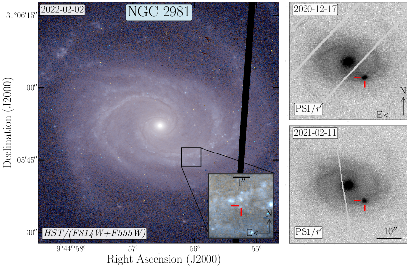
SN 2020acct (ZTF20acwobku) was discovered by the Zwicky Transient Facility (ZTF; Bellm et al., 2019) in the $g$ -band on 2020 December 10 16.75 UT, or MJD 59193.923, at RA=09:44:56.060, $\delta$ =+31:05:45.77. Located in NGC 2981 at $z=0.034650$ (Albareti et al., 2017), SN 2020acct is offset 6.24”S, 6.27”W from the core of the galaxy (a physical separation of 6.1 kpc). The location of SN 2020acct within NGC 2981 is shown in Figure 1. The field of SN 2020acct was also observed as part of routine operations by the Young Supernova Experiment (YSE; Jones et al., 2021), the Pan-STARRS survey for Transients (PSST; Huber et al., 2015) and the Asteroid Terrestrial-impact Last Alert System (ATLAS; Tonry et al., 2018). The YSE-PZ web broker was used for coordinating followup observations and visualisation of the YSE, ATLAS and public ZTF data (Coulter et al., 2022, 2023).

Refer to caption — Figure 1: Images of NGC 2981, the host galaxy of SN 2020acct. Left: Stacked HST images (F275W, F555W and F814W bands). The 3″ $\times$ 3″ inset image zoomsin on the local environment with red crosshairs marking the location of SN 2020acct. Right: PanSTARRS-1 $r$ -band images of SN 2020acct during the first (top) and second (bottom) peaks used for astrometric measurements.

$g$ , $r$ , $i$ , $z$ -band imaging was obtained through YSE with the Pan-STARRS telescope (PS; Kaiser et al., 2002) between 2020 December 09 and 2021 February 22. All images were reduced with the YSE photometric pipeline, which is based on photpipe (Rest et al., 2005), with template images taken from stacked Pan-STARRS1 $3\pi$ sky survey data (Huber et al., 2015, Fulton et al. in prep.). All images and templates are resampled and astrometrically aligned to match a skycell in the PS1 sky tessellation, and nightly image zero-points determined by comparing PSF photometry to PS1 stellar catalogues (Huber et al., 2015). PSF-matched templates are subtracted from the nightly images, and the flux-weighted centroid is determined at a position forced to match the SN position determined from the first images, from which we perform PSF photometry. Additional $i$ , $z$ , $y$ -band Pan-STARRS imaging was obtained as part of PSST, alongside the composite $w$ -band. PSST images were processed in real-time as described in Magnier et al. (2020a). We perform forced photometry at the location of the first Pan-STARRS detection using the Pan-STARRS1 $3\pi$ sky survey data (Huber et al., 2015) as our reference.

We use the ZTF forced photometry server (Masci et al., 2023) to obtain public $g$ - and $r$ -band photometry of SN 2020acct, with detections spanning 2020 December 10 to 2021 April 02 ( $-$ 58 to +50 d in the rest-frame). We use the ATLAS forced photometry server (Tonry et al., 2018; Smith et al., 2020; Shingles et al., 2021) to recover the difference-image photometry in the $o$ - and $c$ -bands for SN 2020acct, with detections covering the period 2020 December 10 to 2021 February 22.

We obtained target-of-opportunity observations from the Neil Gehrels Swift Gamma-ray Burst Mission (Swift; Gehrels et al., 2004) UltraViolet and Optical Telescope (UVOT; Roming et al., 2005). SN 2020acct was monitored with Swift from 2020 December 14 to 2020 December 23, and from 2021 February 12 to 2021 February 23. To estimate the host-galaxy level for subtraction, UVOT observations were also obtained after the SN had faded on 2021 October 11. We perform photometry using the HEAsoft package UVOTSOURCE with a source aperture of 2.0” to minimize contamination from surrounding regions of star formation and a source free background region with a radius of 20.0”.

Observations with the Hubble Space Telescope (HST) WFC3/UVIS of SN 2020acct were obtained in the F275W band on 2021 November 29 (program GO–16657, PI: Fremling), and in the F555W and F814W bands on 2022 February 02 (program SNAP–16691 , PI: Foley). SN 2020acct is undetected at both epochs, with 5 $\sigma$ -limits of $m_{\mathrm{275}}>28.3$ , $m_{\mathrm{555}}>27.8$ and $m_{\mathrm{814}}>27.8$ within a 1” aperture.

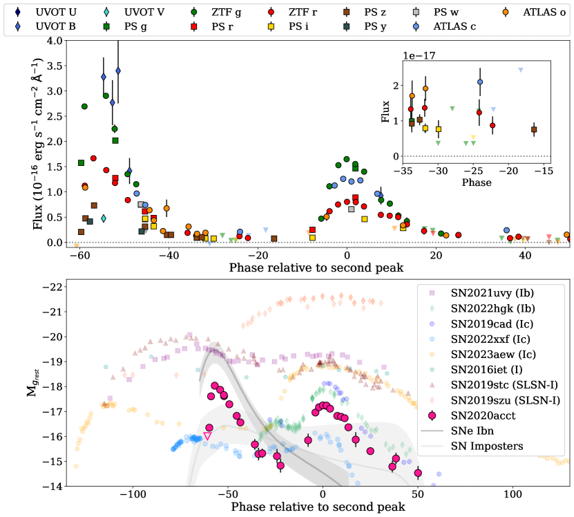
We estimate the time of explosion, $t_{0}=59192.1\pm 0.5$ , as the midpoint between the last pre-explosion non-detection from ATLAS on MJD 59191.58 and an early first detection from the YSE survey in the $g$ - and $z$ -bands on MJD 59192.65. We present the light curve of SN 2020acct in the top panel of Figure 2, with detections spanning 106 rest-frame days from initial discovery. Photometric observations are provided within Appendix Table 1, where all rest-frame phases are reported with respect to the maximum of the second peak. All photometry is corrected for the Milky Way foreground extinction using the dust maps of Schlafly & Finkbeiner (2011). We do not correct for internal host galaxy extinction.

2.1.1 Astrometry

We analyzed PS1 $r$ -band images corresponding to the first and second peaks of SN 2020acct, taken on 2020 December 17 and 2021 February 11, respectively, to determine the relative astrometric offset and confirm the coincidence of the two peaks. The zoomed-in images are displayed in the right panels of Figure 1.

Using Source Extractor (Bertin & Arnouts, 1996), we identified common stars in both images. We applied quality control cuts to exclude stars based on source ellipticity, the full width half maximum (FWHM), saturation, or proximity to the image edges. After removing these sources, the images had 30 stars in common with well-measured positions.

To compute the geometric transformation between the two images, we performed iterative fitting on these stars using GEOMAP (Tody, 1986). Following the removal of 4 additional stars, we applied a second-order Legendre polynomial fit and used GEOTRAN to apply this transformation. We performed additional systematic tests, including a jackknife test with the selected stars to determine the influence of individual stars in the fitting process and, by changing the order of the fit, finding an additional 0.07 and 0.07-pixel uncertainty in each direction, respectively.

We find the location of the two peaks to be coincident, with a relative offset of (0.19 $\pm$ 1.71, 0.36 $\pm$ 1.38) pixels in the $x$ and $y$ dimensions, respectively, or (0.76 $\pm$ 6.84, 1.44 $\pm$ 5.52) arcsec, indicating they are consistent to within 0.19-sigma.

2.1.2 Long-term Light Curve

We search for variability prior to the detection of the first peak of SN 2020acct, performing forced photometry at its astrometric location. We use the ZTF (Masci et al., 2019), and ATLAS (Smith et al., 2020) forced photometry servers to recover the difference-image photometry, and internally collected forced photometry for PSST, with observations dating from 01 Jan 2018 (ATLAS), 18 Nov 2013 (PSST) and 13 Nov 2019 (ZTF). We visually inspect the forced light curves and do not find significant pre-explosion activity within the PSST and ZTF data down to a luminosity of M $=-14.9$ . For the shallower ATLAS data, we compare the forced light curve of SN 2020acct to the forced photometry of eight control light curves located within a circular radius of 15’ of the transient, using the weighted mean of the control light curves to identify any discrepant epochs in the target light curve (see Rest et al., 2024, for further details). We find no significant variability in the pre-explosion data out to MJD 57754 (01 Jan 2017), down to a luminosity of M ${}_{o}=-15.9$ .

2.2 Spectroscopy

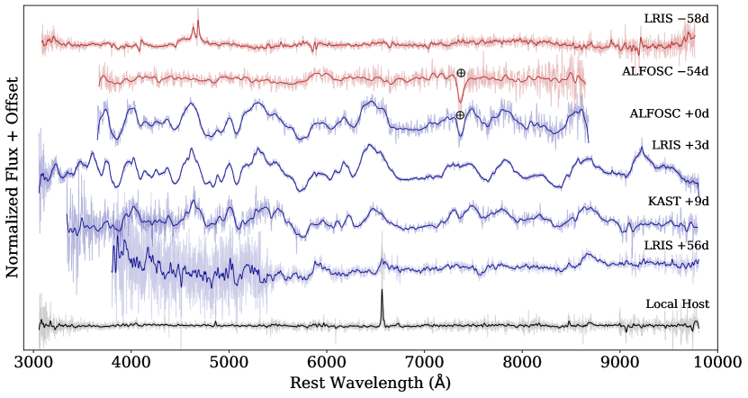
We obtained 5 epochs of optical spectroscopic observations of SN 2020acct spanning $-$ 58 d to +56 d (rest-frame). The optical spectra were obtained with the Kast dual-beam spectrograph (Miller & Stone, 1993) on the Lick Shane telescope, the Alhambra Faint Object Spectrograph (ALFOSC) on the Nordic Optical Telescope (NOT), and the Low-Resolution Imaging Spectrograph (LRIS; Oke et al., 1995) on the Keck I telescope. A final spectrum was obtained using LRIS on 2021 May 12 (+89 d), with the slit centred on the SN location after optical light from the second peak had faded. We use this spectrum for host galaxy corrections. A log of all spectroscopic observations and observing setups are presented in the Appendix.

The LRIS and Kast spectra were reduced using the UCSC Spectral Pipeline¹¹1https:github.commsiebert1UCSC_spectral_pipeline and processed as described in Siebert et al. (2019). The NOT-ALFOSC spectra were reduced using custom built iraf pipelines. We color-correct all transient and host-galaxy spectra, mangling the spectra (Hsiao et al., 2007) to the available photometry to correct for slit losses. We use the LRIS local host galaxy spectrum to perform our host-subtraction, convolving the host spectrum to lower resolution instruments where applicable before subtraction. We present the reduced spectra of SN 2020acct in Figure 3.

3 Analysis

Below we examine the spectroscopic, photometric and host-galaxy properties of SN 2020acct, outlining its physical characteristics in the context of other CCSNe.

3.1 Host Galaxy Environment

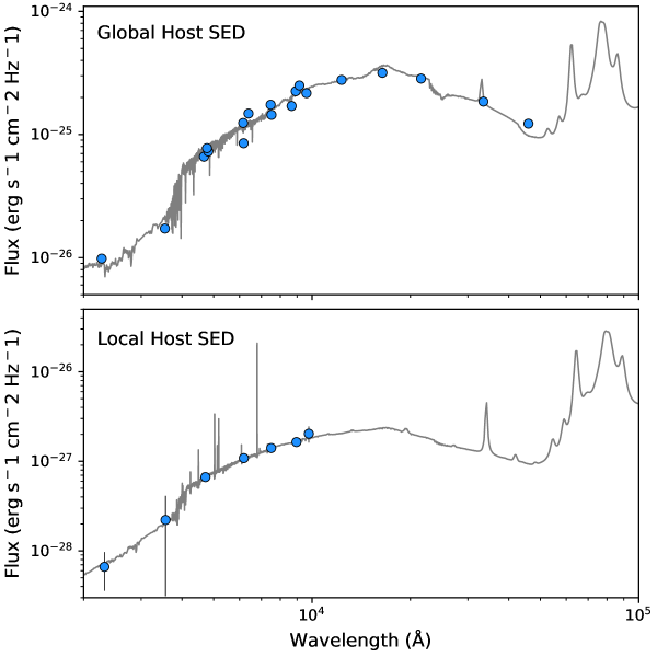
To examine the properties of the host galaxy of SN 2020acct we perform Spectral Energy Distribution (SED) fitting, collecting archival $g$ , $r$ , $i$ , $z$ , $y$ images from the PS1 3 $\pi$ catalog, alongside $J$ , $H$ , $K$ measurements from the 2 Micron All Sky Survey (2MASS; Skrutskie et al., 2006), W1 and W2 bands from the Wide-field Infrared Survey Explorer (WISE; Wright et al., 2010) and NUV and FUV photometry from the Galaxy Evolution Explorer (GALEX; Martin et al., 2005). We measure the global flux of the global host galaxy within a Kron-like aperture (Magnier et al., 2020b) as determined within the PS1 images, applying the same aperture across all survey images and filters for consistency. We also extract the host photometry within a 1” (corresponding to 0.6 kpc) aperture centered on the explosion site of the SN to determine the properties of the stellar population native to the progenitor.

Given that SN 2020acct is located 9.3” from the centre of NGC 2981, we fit both the global and local host photometry using the stellar population synthesis models of Prospector (Leja et al., 2017; Johnson et al., 2021). We apply a 10% error floor to all photometry to account for systematic uncertainties in both the photometry and the physical models being fit to the emission. For fitting the global host photometry, we invoke a model similar to that of Prospector- $\alpha$ detailed by Leja et al. (2017), in which the stellar mass, metallicity, six-component star formation history, and dust fraction, and reprocessing are free parameters (as per Ramsden et al., 2022). In this case, the model uses a non-parametric Dirichlet star formation history (SFH) treatment, but the remaining free parameters used are well described in Leja et al. (2017). For fitting the local environment, we assume an exponentially declining star formation history, with broad priors on stellar mass ( $4<Log(M_{*})<12$ ), star-formation history ( $-2<Log(\tau)<2$ ) and metallicity ( $-4<Log(Z_{\odot})<10$ ). We generate models for both fits which include the effects of stellar and nebular emission, metallicity, dust reprocessing, sampling posterior using the Bayesian nested sampling code dynesty (Speagle, 2020).

Fitting the global SED, we find that NGC 2981 has a stellar mass of $\log{(M_{\star}/M_{\odot})}=11.29^{+0.04}_{-0.06}$ , and a current star formation rate of $(SFR/M_{\odot}yr^{-1})=17^{+15}_{-11}$ . When we fit the SED of the stellar population local to the explosion site aof SN 2020acct, within a 1” radius of its location, we find a local star formation rate of $\log{(SFR/M_{\odot}{\rm yr}^{-1})}=-1.1^{+0.9}_{-0.7}$ and average stellar age of $t_{\mathrm{age}}$ = 9.13 ${}^{+4.5}_{-3.3}$ Myr, from which we infer a local specific star formation rate (sSFR) of $\log{(\mathrm{sSFR/M_{\odot}yr^{-1}})}=-10.4^{+0.8}_{-0.6}$ . We show our global and local SED fits in the Appendix (Fig. 14).

We measure a local gas phase metallicity using emission lines from the LRIS spectrum taken at the location of SN 2020acct. Only H $\alpha$ , H $\beta$ and NII $\lambda$ 6584 lines are observed, for which we measure fluxes of $F_{H\alpha}=4.2\pm 0.2\times 10^{-16}$ erg s^-1 cm^-2, $F_{H\beta}=7.5\pm 0.8\times 10^{-17}$ erg s^-1 cm^-2 and $F_{NII}=6.6\pm 1.4\times 10^{-17}$ erg s^-1 cm^-2. We use the N2 metallicity diagnostic of $12+\log(O/H)$ =8.734 + 0.462 $\times\log([NII/H\alpha])$ (Marino et al., 2013) and find $12+\log(O/H)$ = 8.36 (0.46 $Z_{\odot}$ ). We also estimate the local SFR using the H $\alpha$ line flux diagnostic of (Kennicutt, 1989), and find SFR(H $\alpha)=9.4\times 10^{-3}$ M_⊙ yr^-1. We note that this metallicity ( $\approx 0.4\,Z_{\odot}$ ), approximate to the metallicity of the Small Magellanic Cloud, is significantly lower than the SFR inferred through our local Prospector fitting, but is likely due to differences in aperture-size. Spatially resolved integral-field spectroscopic observations will likely disentangle this issue.

3.2 Spectroscopic Properties

3.2.1 First Peak

From Figure 3 we can see that the spectroscopic properties of the two peaks are very distinct. The higher-resolution LRIS spectrum of the first peak, obtained at $-$ 58 d (approximately $-$ 1 d from maximum of the first peak), displays a blue continuum with several superimposed narrow absorption and emission lines, including strong He I $\lambda\lambda 4471,5857$ Å and He II $\lambda 4686$ Å P-Cygni features. Given the lack of corresponding H $\alpha$ and H $\beta$ emission, we identify the P-Cygni feature at $\lambda 4100$ Å as He II.

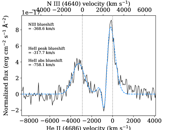
The feature at 4600 Å requires additional examination. This feature has two peaks above the continuum with the redder peak corresponding to He II $\lambda 4686$ Å. The bluer peak is roughly consistent in wavelength with the N III triplet $\lambda\lambda 4634,4640,4641$ , however, we disfavor this identification, as discussed below.

The wings of each peak are much narrower than the Lorentzian (or “IIn-like”) profiles typically seen in either flash-ionized SNe II or SNe Ibn (which are produced by electron-scattering of free electrons as they pass through the ionized CSM; Chugai, 2001; Huang & Chevalier, 2018). If the two peaks were attributed to resolved narrow lines of He II and N III, this would imply a width of $\lesssim$ 1000 km s^-1 (see Appendix Figure 8) and therefore a low optical depth for the line-forming region of the CSM compared to other CCSN progenitors (Jacobson-Galán et al., 2024).

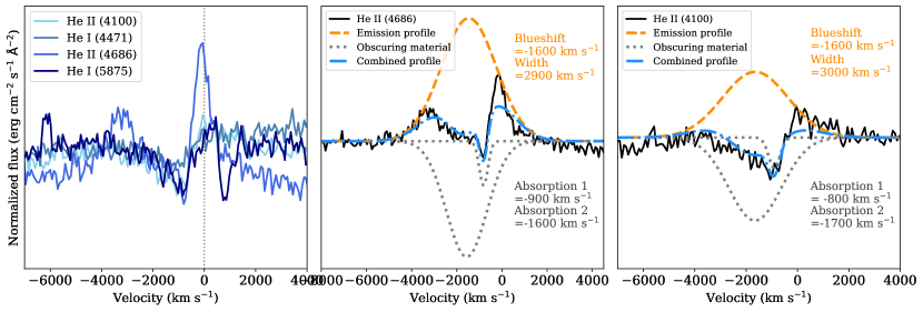
Instead, the 4600Å feature can be explained exclusively as He II with a complex line profile. This profile requires a single emission component blueshifted by -1600 km s^-1 with a FWHM of 2900 km s^-1 and two absorption components at $-900$ km s^-1 and $-1600$ km s^-1. The absorption significantly reduces the core of the emission, separating it into two apparent emission peaks. This is supported by comparison to other He II lines, which exhibit a consistent velocity structure (see for example the He II $\lambda 4100$ Å feature, Fig. 4). The apparent blueshift of these lines from the rest frame ( $\sim$ 1600 km s^-1) may be due to destructive opacity effects (Jerkstrand, 2017), where redwardly scattered photons that are moving toward the observer are suppressed by optically thick interceding material, creating an apparent strong reduction in flux from the red wing of the line.

We thus identify the 4600 Å feature as being produced solely by He II $\lambda 4686$ Å with no N III contribution. Thus the first optical spectrum of SN 2020acct exhibits only He spectral features. These emission features have mostly disappeared by the $-$ 54 d spectrum (+3 d from first maximum), where only broad, weak He I $\lambda 5876$ Å emission is observed.

In Figure 5 we compare the first peak spectrum of SN 2020acct to the those of CCSNe at similarly early epochs ( $<-7$ d). At these phases, nearby CSM is ‘flash-ionized’ by ultraviolet (UV) radiation emitted by the breakout of the SN shock from the stellar envelope (Yaron et al., 2017; Terreran et al., 2022), rapidly cooling and recombining (Gal-Yam et al., 2014; Khazov et al., 2016). We also compare with the early flash-ionization spectra of rapidly evolving SNe Ibn (Pastorello et al., 2015; Gangopadhyay et al., 2020), non-terminal outbursts from SN impostors (Fraser et al., 2013; Brennan et al., 2022), and with spectra of cooling of shock-heated ejecta following shock breakout (shock cooling; SC) in a SN IIb (Tartaglia et al., 2017).

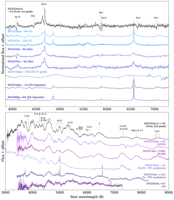
The helium emission features present within the first peak of SN 2020acct do not resemble the broad features produced by rapidly expanding ejecta within SNe, or within SN IIb shock-cooling peaks. The lack of Balmer emission disfavors a SN impostor interpretation for the first peak (also see Sect. 3.3). These features are instead more similar to those of flash-ionized CCSNe and SNe Icn/Ibn, whose features are the result of brief CSM interaction. Though the brevity of the emission features seen in the $-$ 58 d spectra (gone 4 days later) and the presence of high-ionization recombination lines such as He II $\lambda 4846$ Å, are reminiscent of short-lived recombination lines in the early epochs of SNe II (Khazov et al., 2016; Bruch et al., 2023) and some SNe Ibn (Pastorello et al., 2015; Hosseinzadeh et al., 2017; Gangopadhyay et al., 2020). The lack of H $\alpha$ emission and broader line widths (see Fig. 4) present in SN 2020acct suggest a different origin of interaction.

The broad, complex helium line profiles with emission and multi-absorption components, indicate a complex CSM structure. From our simple modeling, the absorption profiles imply that at least two regions of obscuring material sit between the emission zone and the observer in order to mask the center of the He II emission profiles. The lack of corresponding hydrogen absorption suggests that this obscuring CSM is also hydrogen-free. We estimate velocities of approximately $\sim$ -900 km s^-1 and $\sim$ -1600 km s^-1 for these helium absorbing regions. The different widths and velocities of these profiles suggest a complicated geometry with multiple obscuring regions. Understanding the geometry of this CSM structure requires detailed 3D radiative transfer simulations, which is beyond the scope of this work.

3.2.2 Second Peak

Upon re-brightening, the second peak of SN 2020acct exhibits a very different spectral evolution. The strong, broad absorption features visible are characteristic of a stripped envelope supernova (SESN). The lines present at this phase include: He I $\lambda$ 4471,4922,5876,6678 Å, Na I $\lambda$ 5890,5896 Å, O I $\lambda$ 6158,7774 Å, Sc II $\lambda$ 5663,6247 Å, Ca II $\lambda$ 3934 Å and the near infrared (NIR) triplet $\lambda$ 8498,8542,8662 Å, Mg II $\lambda$ 7887 Å, forests of blended Ti II around $\lambda$ 4400 Å, and Fe II lines around $\lambda$ 4550 Å. We also tentatively identify the broad, flat-topped feature around 7300 Å (obscured by a telluric in the +0 d spectrum but clear at +3 d) as a blend of forbidden [Ca II] $\lambda$ 7291,7323 Å and [O II] $\lambda$ 7320,7330 Å, with potential contributions from [Fe II] $\lambda$ 7452 Å or N I $\lambda$ 7468 Å toward the red wing of the feature, with the two wings becoming more distinguished by the +9d spectrum. Notably, SN 2020acct exhibits relatively narrow absorption features. Fitting the O I $\lambda$ 6158 Å and Sc II $\lambda$ 6247 Å features (which we judge to be unblended features) in the +1 and +3 d spectra, we find ejecta expansion velocities of $5800\pm 900$ km s^-1, decreasing to $4300\pm 400$ km s^-1 at +9 d. The origin of the broad emission feature at 6500 Å is unclear. This could be due to H $\alpha$ ; however the implied velocity from the absorption component ( $13,000$ km s^-1) is substantially higher than the bulk of the ejecta, and we do not see any corresponding H $\beta$ emission. Other possibilities include C II $\lambda$ 6580 Å, [O I] $\lambda\lambda$ 6300,6364 Å, [N II] (as suggested for SN 2023aew; Kangas et al., 2024), or some combination of these lines. By +56 d in the late photospheric phase, we see only rest frame emission from Na I, the Ca II NIR triplet, and the ambiguous 6500 Å feature.

In Figure 5 we compare the +3 d spectrum to the spectra of other double-peaked SESNe; SN 2023aew (Kangas et al., 2024; Sharma et al., 2024), SN 2019stc (Gomez et al., 2021), and SN 2019szu (Aamer et al., 2023), to a late-time spectrum of the superluminous SN (SLSN) SN 2015bn (Nicholl et al., 2016), and to the fast evolving SN Ic SN 2005ek (Drout et al., 2013). The features present during the second peak of SN 2020acct are strikingly similar to those of SN 2023aew, and to SN 2015bn, although less broad. The potential presence of forbidden [Ca II] and [O II] at maximum light is unusual for a typical SESN. Forbidden emission lines can only be produced within low-density environments, where collisional de-excitation is unlikely, and thus radiative de-excitation becomes the dominant process. As such, these features typically appear closer to the nebular phase ( $>$ 100 d from explosion), when the ejecta become largely optically thin. SN 2020acct joins a handful of SNe; SN 2023aew, SN 2019szu, SN 2019stc and SN 2018ibb (Schulze et al., 2023), where these features are prominent close to maximum light.

Aamer et al. (2023) explain the early presence of [O II] emission lines in SN 2019szu as the interaction of the SN ejecta with nearby CSM, ejected 120 d before explosion as a result of PPI, a model which has also been invoked to explain the double-peaked light curve of SN 2019stc. We explore this further in Section 5.2.

3.3 Photometric Properties

The two peaks of SN 2020acct are distinct from each other, with emission dropping by 2.8 magnitudes in the $r$ -band within 22 days from the first maximum. In the bottom panel of Figure 2 we compare the photometric evolution of SN 2020acct to other double-peaked SESNe (Gutiérrez et al., 2021; Kuncarayakti et al., 2023; Das et al., 2023; Kangas et al., 2024; Sharma et al., 2024) including three PPISNe candidates (SN 2016eit, SN 2019stc, SN 2019szu; Gomez et al., 2019, 2021; Aamer et al., 2023). We also compare the first peak’s evolution to the SN Ibn template of Hosseinzadeh et al. (2017) and to a SN impostor template (constructed using data from Fraser et al., 2015; Elias-Rosa et al., 2016; Tartaglia et al., 2016; Pastorello et al., 2018; Brennan et al., 2022).

SN 2020acct does not closely resemble any current event within the literature. The 58 d lag between the two peaks is similar to the peak separations in other events, however the clear drop in flux between the peaks is unique. While the second peak of SN 2020acct falls within the typical distribution of normal Ib/Ic SN luminosities (Richardson et al., 2014), it lies toward the faint end of the double peaked SN range. The brighter first peak exceeds the luminosities typical of a SN impostor, and its light curve evolution is more rapid. Although its rapid behavior is closer to that of SNe Ibn (Hosseinzadeh et al., 2017), the differences in spectral properties outlined in Sect. 3.2 (although see Pursiainen et al., 2023, for spectroscopic diversity), and the appearance of a second peak suggests a different origin.

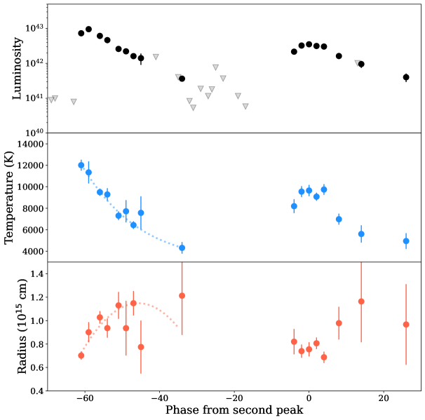
We construct the bolometric light curve of SN 2020acct using the optical foreground extinction-corrected photometry (we exclude Swift photometry due to uncertain background subtraction), grouping data at 2-day intervals and fitting a simple blackbody function to the resulting light curves and integrating across the full blackbody curve to find the bolometric luminosity. We find the luminosity of the first peak to be 9.6 $\pm 0.6\times 10^{42}$ erg s^-1, and that of the second peak to be 3.52 $\pm 0.09\times 10^{42}$ erg s^-1. The flux drops to $<2\times 10^{41}$ erg s^-1 during the minimum between the two peaks.

Examining the blackbody fits (see Figure 7), we find that the first peak of SN 2020acct shows very rapid evolution in both temperature and radius, cooling quickly after peak (cooling by $\gtrsim$ 5000 K in 10 days), with a radius increase of a factor $\sim$ 2 over 10 days to $\gtrsim 8\times 10^{14}$ cm. We also note the unusually large photospheric radius found for both events ( $\gtrsim 8\times 10^{14}$ cm), and seemingly larger for the first peak compared to the second peak. The general behavior is similar to flash-ionized SNe II (though CCSN radii are typically not so extended; Irani et al., 2023), and to Ibn/Icn SNe (e.g. Pellegrino et al., 2022; Pursiainen et al., 2023), where a CSM envelope is quickly shock-heated and then cools.

4 Progenitor Scenarios

We next explore different potential progenitor scenarios to see if they can reproduce the double-peaked light curve of SN 2020acct. We first consider the plausibility of SN 2020acct being the chance occurrence of two individual SNe originating from either the same star-forming region or binary system before exploring models from a single progenitor system.

4.1 Two SNe from the Same Region

We consider a scenario in which the two peaks of SN 2020acct originate from two individual progenitor stars in the same star-forming region, which would appear to be coincident given the localization within the host galaxy.

As the lifetimes of CCSN progenitors are short ( $\sim$ few Myrs), the CCSNe rate should closely follows that of current star formation rate, which we can use to estimate the likelihood of this case. We take the theoretical relationship between SFR and CCSN rate from Botticella et al. (2012). For the local SFR within $\sim 1$ kpc of the explosion site of SN 2020acct, which is $\sim 1\times 10^{-2}$ M_⊙ yr^-1, we would anticipate of order $\sim 10^{-4}$ SNe yr^-1. The probability of two individual SNe occurring within this star-forming region within a 60-day window is thus $\sim 2.7^{-10}$ . The extremely low probability of two SNe occurring within 1 kpc of each other within such a short window suggests this is not a likely scenario to produce SN 2020acct.

4.2 Two SNe from a Binary System

Another possible route to producing two individual SNe at the same explosion site within a short temporal window is to have two progenitors co-evolving within a binary system. Close binary systems, in which Roche-lobe overflow occurs, have been frequently invoked as the progenitors of SESNe, as it presents a more efficient method (compared to stellar winds in single Wolf-Rayet stars) of partially stripping $10-18$ M_⊙ SN progenitors of their hydrogen envelopes (e.g. Claeys et al., 2011; Yoon et al., 2017). Binaries have also been suggested as a mechanism to strip Ibn progenitor envelopes, with some potential direct progenitor detections to support this (Maund et al., 2016; Sun et al., 2020).

However, for a binary system to reproduce the observed properties of both peaks of SN 2020acct, with both components exploding within a $\sim$ 60 day window, both stars within the system must evolve on similar timescales, and undergo sufficient stripping to reduce their outer hydrogen envelopes. A close system in which the binary mass ratio is high may result in unstable mass transfer while both stars are on the main sequence, leading to the formation of a common envelope with a double core (Vigna-Gómez et al., 2018). Within such a system, both stars could co-evolve on more similar timescales while efficiently removing most of their hydrogen envelopes. However, the likelihood of both components reaching the point of final core collapse within 50 days of each other seems implausible.

Another issue with this model is the requirement that enough energy must be lost from the binary system due to its co-rotation within the envelope to sufficiently eject it before both components explode, as we do not observe signatures of strong interaction with a hydrogen-rich CSM within either peak. At the lower end of massive binaries (two 8 M_⊙ stars), the binding energy of the envelope is of order several $\times 10^{49}$ ergs (Kruckow et al., 2016). It may be possible that the explosion of the first component releases sufficient energy to remove any envelope prior to the second explosion. However, from simple modeling (§4.3.3), the kinetic energy released during the first explosion is $\sim(6-8)\times 10^{48}$ ergs, therefore unlikely to be sufficient to eject an envelope alone. It may be possible that some envelope remains after the first explosion, and any signatures of interaction are too weak to be detected while the second SN is bright.

The extreme fine-tuning this scenario would require to evolve both binary components on similar timescales, for the common envelope to be cleanly removed before or by the first SN, and for both cores to collapse within a two-month window, makes this scenario inconceivable. Thus we do not consider this futher as a route to producing the two peaks of SN 2020acct.

4.3 Rate of SN 2020acct-like Events

To help constrain potential progenitor scenarios for SN 2020acct, we determine the observed rate of comparable double-peaked SNe to SN 2020acct. The SN rate is defined as:

R_{\rm 20acct-like}=\frac{N}{f_{\rm spec}\,\epsilon\,VT}

(1)

where $N$ is the number of events observed within a volume $V$ during the time period $T$ . The efficiency of detection (the likelihood that an event is detected within the data of a given survey) is given by $\epsilon$ , while $f_{\rm spec}$ is the spectroscopic completeness of the survey within $V$ .

We estimate the rate of SN 2020acct-like events within ATLAS (our shallowest survey), over a 4-year baseline from 2018-2021, out to a distance of 300 Mpc (z $\sim$ 0.07), beyond which the second peak of SN 2020acct would not have been recoverable within the ATLAS data (and the first peak would be observed as a stand-alone SN Ibn).

Using the ATLAS efficiency simulation tool (which accounts for the survey cadence and 5 sigma limiting magnitudes within a given field), we estimate the recovery efficiency for a SN 2020acct template light curve (see Srivastav et al., 2022, for full details). Assuming an event is efficiently ‘detected’ if a minimum of 10 epochs of co-spatial 5 $\sigma$ detections are recovered, we simulate the efficiency of ATLAS recovery by injecting 10000 events in 50 Mpc bins out to 300 Mpc. From our simulations, we find $\epsilon=0.163$ at 300 Mpc.

To estimate the spectroscopic completeness of ATLAS, we take a similar approach to Nicholl et al. (2023), by selecting all transients detected within the survey of brightness m $<20.0$ (in either the cyan or orange filter) within a 4-year window (2018-2021) and measuring $f_{\rm spec}$ from the ratio of spectroscopically classified to total events with $>11$ ATLAS detections in the light curve (the minimum number of detections required to identify SN 2020acct as a double-peaked event assuming an average ATLAS cadence of 1.5 days). We find $f_{\rm spec}=0.54$ .

Given the changing spectroscopic nature of SN 2020acct, we also search for potentially missed spectroscopically classified events within the 2018-2021 ATLAS data, requiring that candidates have two peaks separated by $>$ 20 days (eliminating IIb shock-cooling curves), and peak luminosities within $\sim 1$ mag of each other, where any spectroscopic classification of either peak matches that of SN 2020acct (signatures of interaction and/or a SESN). We find no other double-peaked events of a similar nature to SN 2020acct.

We measure the rate of double-peaked events like SN 2020acct to be $\sim$ 3.3 $\times 10^{-8}$ events Mpc^-3 yr^-1, approximately $\times 10^{-4}$ of the CCSN rate (Perley et al., 2020; Frohmaier et al., 2021). We thus proceed under the assumption that SN 2020acct is the product of an intrinsically rare progenitor system or explosion mechanism.

4.3.1 Shock Cooling Modelling

A small subset (3-9% Das et al., 2023) of SNe Ib/c have pre-explosion peaks due to the shock-cooling (SC) of extended circumstellar material around the progenitor star heated by the SN shockwave following the initial explosion. We thus model the first peak of SN 2020acct with a SC model, where photons deposited by the shockwave begin to escape from optically thick ejecta or CSM (Waxman & Katz, 2017). SC emission is expected to last on the order of a few days, with a light curve morphology driven by both the energetics of the shock wave and the properties of the nearby CSM (Nakar & Sari, 2010; Waxman & Katz, 2017). We fit the first peak with the revised models of Piro et al. (2021), fitting only optical ( $g,r,z,o$ ) photometry from the first 10-days after our estimated $t_{0}$ , where the model is valid. We find the best fit to these data to be shock cooling of a CSM envelope at a radius of $R_{\rm CSM}$ =750 $\pm$ 10 R_⊙, that has a mass of $M_{\rm CSM}$ =0.20 $\pm$ 0.05 M_⊙, and is moving at a velocity of $v_{e}$ =12,000 $\pm$ 800 km s^-1.

The primary issue with this model is that SC emission does not provide a natural explanation for the delay between the first and second peak, and requires that the SN occur at the beginning of the first peak. It is then difficult to explain the second peak reaching maximum $\sim$ 50 days later.

4.3.2 Low Mass Helium Star Models

Given the presence of helium emission during the first peak, we explore models commonly used to describe the production of SNe Ibn, an intrinsically rare subset of SESN (approximately 1% of all SNe; Pastorello et al., 2008). A massive Wolf-Rayet star which loses all or most of its hydrogen envelope through luminous blue variable (“LBV-like”) outbursts (e.g. Pastorello et al., 2007), winds, or binary interaction can accumulate a substantial helium-rich CSM around the progenitor. Interaction of the final SN ejecta with this CSM (e.g. Foley et al., 2007; Pastorello et al., 2008; Dessart et al., 2022) could potentially power the light curve.

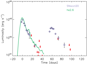
We explore several models involving explosive mass ejection and winds from low mass (initial masses 2-3 M_⊙) helium stars at solar metallicity (see also Dessart et al., 2022). Two examples are shown in the Appendix (Figure 12). One, based on a helium star with initial mass 2.6 M_⊙ (pre-SN mass 2.14 M_⊙) experiences a very low energy terminal explosion ( $2.3\times 10^{49}$ erg), that interacts with a shell ejected by a silicon flash 101 days earlier. The other, a helium star with initial mass 2.7 M_⊙ (pre-SN mass 2.21 M_⊙) experiences no silicon flash, but instead interacts with a very strong wind (0.1 M_⊙ yr^-1). Such a large mass loss rate might be reasonable for a star that is burning oxygen and silicon during the last year of its life in unstable flames bounded by a molecular weight inversion (Woosley, 2019), or perhaps late-stage binary interaction.

While both models are capable of reproducing the first peak of SN2020acct, each has some deficiencies. Models invoking interaction of a terminal explosion with a previously ejected shell require very low explosion energies ( $2.3\times 10^{49}$ erg) to avoid making the light curve too bright. Reducing the wait time between the silicon flash and core collapse could produce a fainter event, but then the SN ejecta would also overtake the ejected shell before peak luminosity was reached, resulting in no narrow emission lines. Moreover, this model does not offer a natural explanation for the presence of the second peak.

The simplest wind model produces a light curve that declines too slowly following the first peak. This could reflect the decreasing optical efficiency of the forward shock as it moves outside the photosphere or a variable mass loss rate. In particular, if the mass loss rate increased with time just before the explosion, the density in the wind would decline more steeply than $r^{-2}$ . This model also does not provide an intuitive explanation for the second peak. While a composite model invoking an interaction with a shell of material ejected by a silicon flash prior to the wind phase is possible, the lack of narrow lines during the second peak discredits this.

While these models arise from a more instinctive progenitor population given the host environment of SN 2020acct (see Sect. 3.1), they critically cannot explain the presence and properties of the second peak. We thus do not consider these models further here.

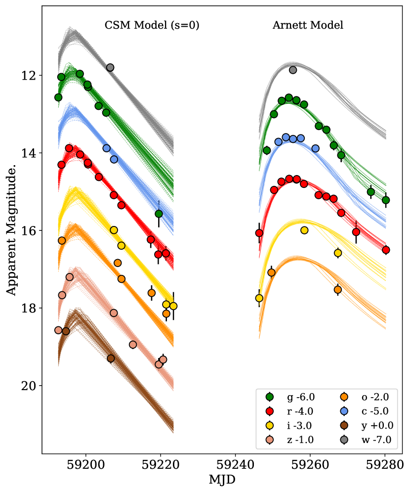
4.3.3 MOSFiT Modelling

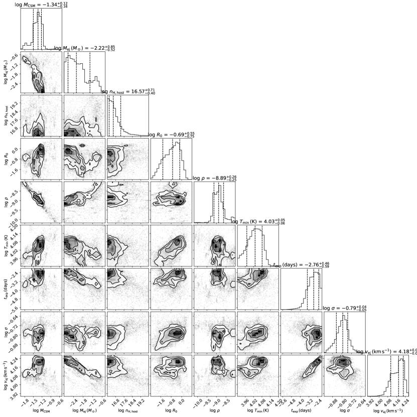
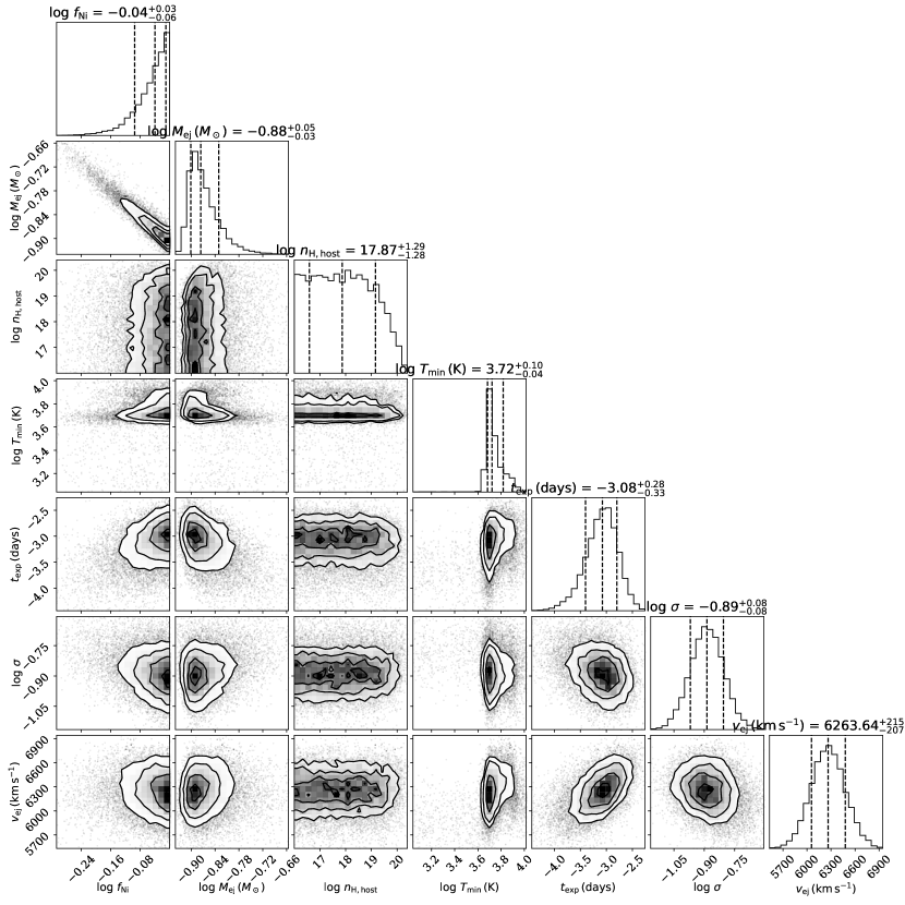
We use the Modular Open Source Fitter for Transients (MOSFiT) code (Guillochon et al., 2018) to estimate the likely explosion parameters for each peak under the assumption that the first peak is CSI-powered (Chatzopoulos et al., 2012; Jiang et al., 2020) and the second is the result of Ni⁵⁶ decay model (Arnett, 1982). We select data within the MJD range 59192.65 - 59223.43 for the first peak and in the range 59248.40 - 59280.27 for the second peak, independently fitting the two models but allowing for the explosion epoch of the second to coincide with the first peak. For the CSI modeling, we explore different CSM density profiles ( $\rho_{\mathrm{CSM}}$ ), where the density is a power law function of the radius, $r$ , such that $\rho_{\mathrm{CSM}}\propto r^{-s}$ . We fit the peak three times under the assumption of (i) a shell-like CSM ( $s=0$ ), (ii) a wind-like CSM ( $S=2$ ), and (iii) with $s$ as a free parameter. To efficiently sample our posterior parameter space, we use the Bayesian nested sampling code dynesty (Speagle, 2020).

Overall we find that the CSI and the Ni⁵⁶ decay models provide agreeable fits to the data. In particular, the CSM interaction model is able to capture the swift rise and slower decline of the first peak, although with a very low CSM mass of 0.05 M_⊙ and 7 $\times 10^{-3}$ M_⊙ of ejecta. We find negligible differences in the goodness of fit when using a wind-like and a shell-like CSM, and leaving this parameter free does not suggest a preference either way. However, as the CSI models implemented within MOSFiT are based on the analytic models of Chatzopoulos et al. (2012), which assume a continuous, power-law density profile for both ejecta and CSM, these unusual values may be a result of trying to fit a simple model to a more complex physical scenario. For the second peak, we find good fits to the Ni⁵⁶ decay models involving 0.1 M_⊙ of ejecta with an extremely high nickel fraction (f ${}_{\rm Ni}=0.91$ ). Such low ejecta mass is unusual for a SESN. SNe Ibc typically eject between 2-4 M_⊙ of material (Drout et al., 2011; Lyman et al., 2016), of which 0.08 M_⊙ on average is Ni⁵⁶ (Afsariardchi et al., 2021). Though Arnett Ni⁵⁶ masses are usually overestimated (Afsariardchi et al., 2021), the low ejecta mass and unrealistically high Ni⁵⁶ could indicate that the second peak is not produced by a standard SESN progenitor. Our assumed model priors and resulting fit parameters can be found in Appendix Table 3 and our fit shown in Appendix Figure 9.

4.4 Discussion

Based on its spectroscopic properties exhibited by both peaks and the results of our MOSFiT modeling, it is reasonable to assume that the first peak of SN 2020acct is powered solely by CSM interaction. Additionally, the MOSFiT results imply that the second peak explosion date occurs after the first peak has faded, and its spectral evolution is similar to that of a SESN powered by Ni⁵⁶ decay (although the unrealistically high nickel fraction and low nickel mass make this scenario unlikely, see Section 5 for further discussion).

However, both peaks of SN 2020acct present distinct properties that make their origins difficult to reconcile with normal SN models. The second peak of SN 2020acct appears to be a terminal explosion, both from its spectroscopic properties and from its photometric and spectroscopic similarity to SESNe. Despite its spectroscopic similarity to SESNe and alongside light curve properties concurrent with the other events within this class, the relatively low expansion velocities of the ejecta, alongside the early emergence of forbidden [Ca II] and [O II] lines typically observed at the nebular phase, suggest a different progenitor origin to a typical SESN.

The first peak is equally problematic. Its spectroscopic features suggest strong interaction with nearby hydrogen-free CSM, although its duration and luminosity make it difficult to reconcile as either a stand-alone SN or as a SN impostor. Its separation in time from the second peak (58 d in the rest frame) puts it at odds with shock-cooling models from shock-breakout at the onset of core collapse, and from models invoking CSM interaction from explosions of low-mass helium stars. In particular, if originating from the same explosion, the separation between the two peaks is seemingly too long for them to be causally connected (i.e. the onset of core collapse cannot happen long before the start of the second peak). The strong, broad helium emission lines imply a different CSM configuration to the nearby CSM illuminated during the early phases of normal CCSNe and SNe Ibn.

PPISN is a very appealing scenario to describe SN 2020acct, as its properties align with the key hallmark of PPISNe - the presence of an interaction-powered transient with SN-like energies prior to a terminal explosion. PPI would provide a natural explanation for the two luminous and distinct peaks of the event, whilst the low observed rate of similar events measured within ATLAS would agree with the natural rarity of PPI progenitors (estimated to be a few in a thousand of all CCSN progenitors Vigna-Gómez et al., 2019). We explore a PPI progenitor scenario for SN 2020acct more in the following section.

5 Pulsational Pair Instability

Episodic eruptive mass-loss in massive stars has been shown to produce luminous precursory peaks within SN light curves (Smith et al., 2010; Fraser et al., 2013; Smith, 2014; Bilinski et al., 2015; Elias-Rosa et al., 2016). However, the luminosity (peaking on average at $\sim 10^{42}$ erg s^-1), evolutionary timescale and distinct spectroscopic features of the first peak make it unlikely that the first peak arises due to an LBV-like eruption as seen in SN impostor events. The absence of hydrogen in the first peak spectra of SN 2020acct also makes it difficult to explain as an LBV eruption.

PPI presents one possible way of producing a peak powered purely by helium-rich CSM interaction without needing to invoke an underlying SN. Collisions of ejected shells of material are capable of powering transients ranging between $10^{41}-10^{44}$ erg s^-1 (Woosley, 2017; Renzo et al., 2020a), prior to the onset of final core collapse. However, due to the requirement of large initial masses to build a sufficiently massive core, stars which experience PPI are expected to be intrinsically rare, thus the rate of PPISNe should be low (Renzo et al., 2020a).

In this section, we compare the light curve of SN 2020acct to PPI models of single helium cores and explore the feasibility of this progenitor scenario with regard to its observed properties and its host environment.

5.1 PPI Models

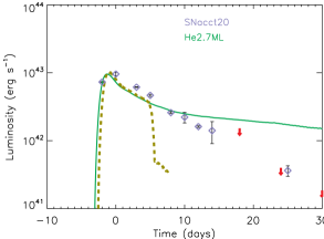
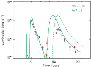
Theoretical models suggest that PPI is capable of reproducing a wide variety of light curve morphologies and spectra (Heger & Woosley, 2002; Moriya & Langer, 2015; Woosley, 2017; Renzo et al., 2020a). For single-star models, this observational diversity is a result of differences in the efficiency of stripping the outer hydrogen envelope, while the number of pulses is governed by the energetics of the initial pulse (such that more energetic pulses are less frequent). For stars $\gtrsim 40$ M_⊙, pulses from PPI are expected to completely remove the outer hydrogen envelope of the progenitor, leaving only a bare He core at the point of collapse. Early emission is expected in PPI events as a result of colliding shells of ejected material. In cores $>$ 44 M_⊙, the pulse interval should become long enough ( $\sim$ several days) that individual peaks will be discernible in the light curve, although above $\gtrsim$ 52 M_⊙, the delay between the pulses are too far apart in time to produce bright collisions with the first ejected material (Woosley, 2017).

For a star stripped of its hydrogen envelope, the observed duration of the double-peaked light curve (at least 60 d), qualitatively agrees with models of helium core masses entering PPI of $\sim$ 50 M_⊙ (Woosley, 2017, see Fig. 5), which we use as the basis for our modeling here. Including the additional mass ejection episodes to create the circumstellar shell that produces the narrow lines in the first peak, the upper limit on this helium core mass is about 53 M_⊙ (for the nuclear reaction rates assumed in Woosley, 2017). These core masses correspond to larger helium star masses when the core is first uncovered, either via winds or binary interaction, with the actual values dependent on metallicity and an uncertain mass loss rate. Assuming a metallicity 10% solar and the WR mass loss rates of Yoon et al. (2017), the initial helium core mass would be $70-73$ M_⊙, corresponding to a Zero Age Main Sequence mass of $\sim 140-150$ M_⊙ (Woosley, 2019). In this mass range, the PPI models transition from those which experience multiple pulses (50 M_⊙ models), each with a peak luminosity $\sim$ 10⁴³ erg s^-1, to just a single major outburst (cores $>$ 53 M_⊙). In more massive cores the initial pulses are stronger, resulting in a longer delay until the final death of the star, but also burning more of the carbon and oxygen within the core. As a result, the final pulses are fewer and weaker. An uncertain, but diminishing mass of carbon also acts to decelerate the collapse, weakening the pulses²²2Uncertainties in convection (Renzo et al., 2020a) could have a similar, or even larger, dampening effect..

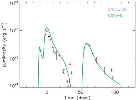
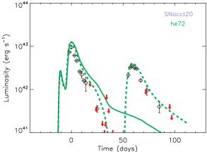
Here we compute models of helium stars with helium core masses at the onset of PPI in the range $51-53$ M_⊙ using the kepler code (Weaver et al., 1978; Woosley, 2017), assuming a metallicity of 10% solar, evolved with mass loss (mass loss models as per Woosley, 2019). To encapsulate the relative luminosity and separation of the two peaks of SN 2020acct, we modify the reaction rates from Woosley (2017) by a factor of 1.2 compared to the default 3 $\alpha$ and ¹²C( $\alpha,\gamma$ )¹⁶O reaction rates to increase the carbon mass fraction at central helium depletion to 0.124. This variation is allowed by uncertainties in the rates (Woosley & Heger, 2021), and acts to shorten the delay between the initial pulse and the death of the star. We add an additional degree of freedom by allowing the shock energy and interval between the peaks to vary by artificially varying neutrino energy losses, which act to shorten the cooling time between pulses. We demonstrate the effects of these adjustments in the Appendix (Fig. 13). A detailed discussion of these models will be presented in Woosley et al. (in preparation.). We present our best fitting model (‘he72’) in Figure 6, in which pulsations of a helium core of 72 M_⊙ (corresponding to core mass at the point of PPI of 52.92 M_⊙) are found to recreate the two peaks of SN 2020acct.

In our best-fitting model, the modified core experiences 5 pulses before collapse. The first pulse, powered mostly by explosive carbon burning, reaches a maximum central temperature of 2.96 $\times 10^{9}$ K, ejecting 0.90 M_⊙ of material, with a kinetic energy 7.7 $\times 10^{49}$ erg. This mass ejection is faint, as no significant radioactive material is ejected and adiabatic expansion reduced the energy deposited by the shock. Most of the energy from nuclear burning ( $\sim 2\times 10^{51}$ erg), goes into expanding the star, reducing its central temperature, after some oscillations, to 8.45 $\times 10^{8}$ K. At this low temperature, it requires 11 years of neutrino-mediated Kelvin-Helmholtz evolution for the core to once again become hot enough to be unstable. During this, most of the energy deposited by the first pulse is radiated away as neutrinos.

Pulses 2, 3, and 4 then occur in rapid succession, separated by only 0.46 days and 3.3 days, respectively (reaching core temperatures of 3.11, 3.31, and 3.89 $\times 10^{9}$ K). Combined, these three quick pulses eject 3.90 M_⊙ of material with a kinetic energy of 3.8 $\times 10^{50}$ erg. Once again, the majority of the nuclear energy goes into the expansion of the star. It is the collision of pulse 4 with the combined ejecta of pulses 2 and 3 that produces the first peak of SN 2020acct. After these last three pulses, the central temperature of the core is 1.23 $\times 10^{9}$ K. At this temperature, the associated waiting time until the death of the star in the unmodified model would be 110 days. Here we temporarily increase the neutrino losses³³3Neutrino losses scale with temperature as $\propto\,T^{14}$ . by a factor of 1.8, which shortens the waiting by 61 days (see Fig. 13), and introduces a weak additional fifth pulse.

The fifth and final pulse reaches a temperature of 5.8 $\times 10^{9}$ K and then rebounds weakly, producing an out-going shock of only about 2 $\times 10^{49}$ erg (corresponding to a luminosity of 4 $\times 10^{42}$ erg s^-1, comparable with the second peak of SN 2020acct). This weak pulse ejects an additional 0.6 M_⊙ of material at low velocity, before the core finally collapses 30 minutes later, producing a black hole with baryonic mass 47.5 M_⊙. For many other models of similar core mass, a slightly higher final bounce temperature is produced ( $\sim$ 6 $\times 10^{9}$ K), which causes the core to immediately collapse into a black hole. It is also possible that this immediate collapse followed by low-level accretion could power an additional weak outburst, but without additional assumptions, there would be no second peak in the light curve (Woosley et al. in prep.).

This model presents a good overall fit to the bolometric light curve of SN 2020acct in Figure 6. We note that the weak peak prior to the first major peak (luminosity $\sim$ 2 $\times 10^{42}$ erg s^-1) is due to the collision of the closely spaced pulses 2 and 3, and may not be present given uncertainties in timing due to neutrino cooling. Given these additional uncertainties and parameters necessary to the ‘modified’ model, we treat the he72 model as suggestive of the ability to describe SN 2020acct as a PPISN, rather than a final solution.

5.2 Consistency with Observed Properties

Both qualitatively and quantitatively, SN 2020acct fits the description of PPI well. The light curve shows a strong match to PPI from a 72 M_⊙ helium core in which a shell-shell collision is observed from material ejected in a combination of three pulses which occurred 64 days prior to the final collapse of the core. We note the large difference in the inferred CSM mass from MOSFiT modeling (0.05 M_⊙) of the first peak and the total CSM mass from shells 2, 3, and 4 (3.9 M_⊙), whose collisions produce the first peak in our radiative transfer models. This difference is likely to arise from the inefficient conversion of kinetic energy to optical radiation within the PPI model, combined with the density structure of the CSM. If the location of the photosphere is not reflective of where the bulk of the ejected material is, analytical light curve models where the luminosity follows the forward shock may not accurately trace all of the ejected CSM for a PPISN.

The photospheric radius and effective temperature for the first peak of the PPI model are 6 $\times 10^{14}$ cm and 15,000 K, respectively. While preliminary (pending a more careful treatment of radiation transport), these values agree with the properties of SN 2020acct (Appendix Figure 7). The interacting, fast-evolving spectroscopic features of the first peak, with strong helium emission, can be explained under shock heating of colliding shells of CSM. PPI typically predicts shell velocities of $2000-4000$ km s^-1 (Woosley, 2017), which would agree with the widths of the unobscured profiles from our modeling in Section 3.2. The absorbing material in front of the photosphere could originate from material ejected from the progenitor in previous outbursts. While the inferred velocities of the absorbing material ( $\sim 900$ km s^-1 and $\sim 1600$ km s^-1) are not entirely consistent with the shell velocity predictions of the PPI model. However, uncertainties in the assumptions behind the symmetry of the pulse or the efficiency of the ejection may reconcile these.

From both PPI modeling and simple blackbody fitting, we can see that the apparent photosphere occurs at much larger radii ( $6\times 10^{14}$ cm) than typically assumed for a CCSN ( $\sim 10^{14}$ cm; Irani et al., 2023), indicating farther removed material than that involved with normal interacting CCSNe. The unusual properties of the second peak can also be accounted for under PPI. The early presence of forbidden [Ca II] and [O II] emission could originate from the SN ejecta crossing the radius at which the shell collision occurred, interacting with the low-density CO-rich material ejected by earlier pulses. Forbidden line features have also been observed within the double-peaked PPISN candidates SN 2019stc (Gomez et al., 2021) and SN 2019szu (Aamer et al., 2023), the latter in particular within its early (near maximum light) spectra, similar to SN 2020acct.

5.3 Environment and Progenitor

PPI can provide an intuitive explanation for the two distinct peaks of SN 2020acct. We now investigate whether the local environment of SN 2020acct is consistent with PPI models. As PPI requires massive helium cores for pair production (M ${}_{\rm He}>\sim$ 30 M_⊙), we typically expect to find PPISN progenitors within low metallicity environments (Yusof et al., 2013; Vink, 2018), and given their expected short lifetimes ( $\sim$ Myrs), typically associated with regions of strong star formation. The local 1” radius environment around SN 2020acct presents average star forming properties compared to the bulk CCSN population (Irani et al., 2022), and a relatively low sSFR for a CCSN host. From the host galaxy spectrum we estimate a local metallicity (as per Storchi-Bergmann et al., 1994), and find it to be 12+log(O/H)=8.36, or 0.4 Z_⊙. While this estimate is sub-solar, it is still significantly higher than the $\sim$ 10% solar metallicity assumed in most single-star PPI models (Yoshida et al., 2016; Woosley, 2017; Renzo et al., 2020a).

However, it has been suggested by Vigna-Gómez et al. (2019) that helium cores massive enough to reach the PPI threshold may be formed via the merger of a binary system composed of less massive stars (ZAMS between $40-64$ M_⊙). After an extended period of hydrogen fusion in both stars cores, the two stars merge to form a single star whose newly combined helium core is sufficiently massive to be unstable to PPI, and will later undergo pulsations. Vigna-Gómez et al. (2019) invoke this model as a potential route to producing PPISN where the progenitors retain more of their hydrogen envelope, than within single-star models of the same core mass for a given metallicity. Thus binary mergers may provide a route to produce PPISN under higher metallicity conditions without needing to form an exceptionally massive single star progenitor in situ.

To estimate the probability of producing a 72 M_⊙ helium core within the local host environment of SN 2020acct, we use the physical properties inferred from our PPI modeling to search for potential progenitor systems within the Binary Population and Spectral Synthesis data release (BPASSv2.2.2; Eldridge et al. 2017; Stanway & Eldridge 2018; Stevance et al. 2020). Assuming a metallicity of $Z=0.004$ , ( $0.4\,Z_{\odot}$ ) we set the hydrogen mass to M ${}_{\mathrm{H}}<0.01$ M_⊙ and the hydrogen mass fraction to $X<0.001$ (i.e. hydrogen-stripped cores; Dessart et al., 2012). We then search for models between 70 and 75 M_⊙. Weighting the models by the Initial Mass Function of Kroupa (2001) and binary fractions and period distributions of Moe & Di Stefano 2017, we find 0.7 systems per million solar masses that meet the above criteria at this metallicity. Though these stars are predicted to be within binary systems, none are the result of a merging system.

Though we do not place any constraints upon the ejecta mass of the final SN within the models of our BPASS search, we find that the average IMF weighted ejecta mass to be $M_{\rm ej}=5.54$ M_⊙. Pulsations are not modelled within the BPASS framework, however this ejecta mass agrees with the estimated total mass lost from pulsations (5.4 M_⊙).

Using the double-Schechter galaxy stellar mass function of Wright et al. (2017) to determine the total mass of galaxies, and assuming that the main sequence lifetime scales with stellar mass as $t\propto M^{-2.5}$ , we calculate the rate from transients originating from a 72 M_⊙ helium core to be $1.1\times 10^{-8}$ events Mpc^-3 yr^-1. This is in agreement with the upper limit of our measured rate from ATLAS. Both our ATLAS rate and estimate from viable BPASS progenitor models are approximately an order of magnitude lower than theoretical predictions from Vigna-Gómez et al. (2019), who estimate PPISN from binary mergers should be a few for every thousand CCSNe. Though a merged binary system provides an easier route to producing the required core mass for PPI within the host galaxy environment of SN 2020acct, it is not impossible that the progenitor was produced within a pocket of low metallicity within the galaxy, in which a single massive (M ${}_{\rm ZAMS}\approx$ 150 M_⊙) progenitor is more easily born. High-resolution environmental studies, in which the very local ( $\sim$ 10’s pc) environment to SN 2020acct can be probed, are the best way to determine the feasibility of this latter scenario (Angus et al. in prep.).

6 Conclusions

We have presented the photometric and spectroscopic follow-up of the unusual transient SN 2020acct in NGC 2981 at $z=0.034$ . This event shows a distinct double-peaked light curve, with peaks separated by 58 d in the rest frame, both astrometrically coincident within the same region of a massive host galaxy. The first peak is more luminous and rapidly evolving, exhibiting strong helium emission lines in its spectra, which disappear quickly. The second peak shows behavior similar to a SESN, but with relatively low expansion velocities and forbidden lines around maximum light. From our analysis of the data and exploration of possible progenitor scenarios, we conclude the following:

•

The properties of the first peak of SN 2020acct are consistent with a transient powered by hydrogen-poor CSM interaction. Spectroscopically it most closely resembles an interacting hydrogen-poor SNe Ibn, although its helium emission features, partially obscured by foreground helium CSM, are much broader than typical Ibn events. Modeling the photometric properties of the peak suggests this interaction occurs at some distance ( $8\times 10^{14}$ cm) from the progenitor.
•

The second peak shows signatures of a terminal stellar explosion, i.e. absorption features similar to SNe Ibc. The presence of forbidden [Ca II] and [O II] lines around maximum light indicate the presence of low-density, pre-burnt material external to the explosion, being swept up with the SN ejecta.
•

We find the rate of double-peaked events like SN 2020acct to be $\sim$ 3.3 $\times 10^{-8}$ events Mpc^-3 yr^-1 at $z=0.07$ ( $\sim 0.001$ % of the CCSN rate).
•

We do not find it likely that SN 2020acct is the random occurrence of two SNe from within the same star-forming region of NGC 2981, given the relatively low star formation rate of the local environment.
•

We rule out the possibility that SN 2020acct originates from the rapid successive explosions of stars within a close binary system. Though binary co-evolution can evolve two stars on a similar timescale, significant tweaking would be required to reproduce the observed properties and explosion times of both peaks.
•

The interaction of a low mass $2.5-3.0\,M_{\odot}$ helium star with its late-stage wind and/or mass ejections is deemed an unlikely progenitor route, given the inability of these models to produce a secondary peak without signatures of interaction.
•

We pose that SN 2020acct may be a candidate PPISN, with the first peak being driven by shock collision of previously ejected shells of material. We fit the bolometric light curve of SN 2020acct with models of helium core explosions, and find that it can be described well with pulsations of a 72 M_⊙ core.
•

The relatively metal-rich and low-star-forming nature of the local host environment seems at odds with a PPI interpretation. BPASS models indicate that 0.7 stripped helium cores of the necessary mass are created per million solar masses of material within such environments. These progenitor numbers are in approximate agreement with the measured upper limit to the rate of SN 2020acct-like events from ATLAS. It is unclear whether such PPI progenitors may be formed in situ at higher metallicity, or must be produced via close binaries mergers (e.g. Vigna-Gómez et al., 2019), with further detailed studies of the local environment required to settle the discrepancy.

The increased survey volume from Rubin Observatory Legacy Survey of Space and Time (LSST) will boost the transient discovery rate by an order of magnitude, while also enabling the detection of faint light curve structures such as pre-explosion outbursts fainter than that in SN 2020acct. Identification and follow-up of double-peaked SNe from Rubin will improve our understanding of the rate of PPISNe, the diversity in their properties, and the range of metallicities that can support them. Since these massive stars are likely the progenitors of at least some of the black holes detected through gravitational wave emission, follow-up of PPISN candidates will provide a powerful, orthogonal constraint on the evolutionary pathways for these systems.

C.R.A. thanks S. Srivastav for the excellent pun contributions to the title of this work. C.R.A., M.N. and A.A. are supported by the European Research Council (ERC) under the European Union’s Horizon 2020 research and innovation programme (grant agreement No. 948381) and by UK Space Agency Grant No. ST/Y000692/1. The UCSC team is supported in part by NASA grant 80NSSC20K0953, NSF grant AST–1815935, STScI grant HST-SNAP-16691, the Gordon & Betty Moore Foundation, the Heising-Simons Foundation, and by a fellowship from the David and Lucile Packard Foundation to R.J.F. V.A.V. acknowledges support by the National Science Foundation through AST–2108676 and under Cooperative Agreement PHY–2019786. M.P. acknowledges support from a UK Research and Innovation Fellowship (MR/T020784/1). P.R. acknowledges support from STFC grant 2742655. H.F.S. is supported by the Eric and Wendy Schmidt A.I. in Science fellowship. M.R.S. is supported by the STScI postdoctoral fellowship. A.G. is supported by the National Science Foundation under Cooperative Agreement PHY–2019786 (The NSF A.I. Institute for Artificial Intelligence and Fundamental Interactions, http://iaifi.org/). A.C. acknowledges support from ANID’s Millennium Science Initiative through grant AIM23-0001. M.R.D. acknowledges support from the NSERC through grant RGPIN-2019-06186, the Canada Research Chairs Program, and the Dunlap Institute at the University of Toronto. C.G. and D.F. are supported by a VILLUM FONDEN Young Investigator Grant (project number 25501), and by research grants (VIL16599, VIL54489) from VILLUM FONDEN. G.N. gratefully acknowledges NSF support from AST–2206195, and a CAREER grant AST–2239364, supported in-part by funding from Charles Simonyi, and OAC–2311355, DOE support through the Department of Physics at the University of Illinois, Urbana-Champaign (13771275), and support from the HST Guest Observer Program through HST-GO-16764. and HST-GO-17128 (PI: R. Foley). S.J.S. acknowledges a Royal Society Fellowship and grants ST/Y001605/1. Parts of this research were supported by the Australian Research Council Discovery Early Career Researcher Award (DECRA) through project number DE230101069. The Young Supernova Experiment (YSE) and its research infrastructure is supported by the European Research Council under the European Union’s Horizon 2020 research and innovation programme (ERC Grant Agreement 101002652, PI K. Mandel), the Heising-Simons Foundation (2018-0913, PI R. Foley; 2018-0911, PI R. Margutti), NASA (NNG17PX03C, PI R. Foley), NSF (AST–1720756, AST–1815935, PI R. Foley; AST–1909796, AST-1944985, PI R. Margutti), the David & Lucille Packard Foundation (PI R. Foley), VILLUM FONDEN (project 16599, PI J. Hjorth), and the Center for AstroPhysical Surveys (CAPS) at the National Center for Supercomputing Applications (NCSA) and the University of Illinois Urbana-Champaign. Pan-STARRS is a project of the Institute for Astronomy of the University of Hawaii, and is supported by the NASA SSO Near Earth Observation Program under grants 80NSSC18K0971, NNX14AM74G, NNX12AR65G, NNX13AQ47G, NNX08AR22G, 80NSSC21K1572, and by the State of Hawaii. The Pan-STARRS1 Surveys (PS1) and the PS1 public science archive have been made possible through contributions by the Institute for Astronomy, the University of Hawaii, the Pan-STARRS Project Office, the Max-Planck Society and its participating institutes, the Max Planck Institute for Astronomy, Heidelberg and the Max Planck Institute for Extraterrestrial Physics, Garching, The Johns Hopkins University, Durham University, the University of Edinburgh, the Queen’s University Belfast, the Harvard-Smithsonian Center for Astrophysics, the Las Cumbres Observatory Global Telescope Network Incorporated, the National Central University of Taiwan, STScI, NASA under grant NNX08AR22G issued through the Planetary Science Division of the NASA Science Mission Directorate, NSF grant AST-1238877, the University of Maryland, Eotvos Lorand University (ELTE), the Los Alamos National Laboratory, and the Gordon and Betty Moore Foundation. Parts of this research are based on observations made with the Nordic Optical Telescope (programme 62-507; PI Angus) owned in collaboration by the University of Turku and Aarhus University, and operated jointly by Aarhus University, the University of Turku and the University of Oslo, representing Denmark, Finland and Norway, the University of Iceland and Stockholm University at the Observatorio del Roque de los Muchachos, La Palma, Spain, of the Instituto de Astrofisica de Canarias. Data presented here were obtained in part with ALFOSC, which is provided by the Instituto de Astrofisica de Andalucia (IAA) under a joint agreement with the University of Copenhagen and NOT. A subset of the data presented herein were obtained at the W. M. Keck Observatory. NASA Keck time is administered by the NASA Exoplanet Science Institute. The Observatory was made possible by the generous financial support of the W. M. Keck Foundation. The authors wish to recognise and acknowledge the very significant cultural role and reverence that the summit of Maunakea has always had within the indigenous Hawaiian community. We are most fortunate to have the opportunity to conduct observations from this mountain. Research at Lick Observatory is partially supported by a generous gift from Google. This research is based on observations made with the NASA/ESA Hubble Space Telescope obtained from the Space Telescope Science Institute, which is operated by the Association of Universities for Research in Astronomy, Inc., under NASA contract NAS 5–26555. These observations are associated with programs GO–16657 and SNAP–16691. This work has made use of data from the Asteroid Terrestrial-impact Last Alert System (ATLAS) project. ATLAS is primarily funded to search for near earth asteroids through NASA grants NN12AR55G, 80NSSC18K0284, and 80NSSC18K1575; byproducts of the NEO search include images and catalogs from the survey area. The ATLAS science products have been made possible through the contributions of the University of Hawaii Institute for Astronomy, the Queen’s University Belfast, and the Space Telescope Science Institute. Based on observations obtained with the Samuel Oschin Telescope 48-inch and the 60-inch Telescope at the Palomar Observatory as part of the Zwicky Transient Facility project. ZTF is supported by the National Science Foundation under Grant Nos. AST-1440341, AST-2034437, and a collaboration including Caltech, IPAC, the Weizmann Institute for Science, the Oskar Klein Center at Stockholm University, the University of Maryland, the University of Washington, Deutsches Elektronen-Synchrotron and Humboldt University, the TANGO Consortium of Taiwan, the University of Wisconsin at Milwaukee, Trinity College Dublin, Lawrence Livermore National Laboratories, and IN2P3, France. Operations are conducted by COO, IPAC, and UW. This research is based on observations made with the Galaxy Evolution Explorer, obtained from the MAST data archive at the Space Telescope Science Institute, which is operated by the Association of Universities for Research in Astronomy, Inc., under NASA contract NAS 5–26555. This publication makes use of data products from the Two Micron All Sky Survey, which is a joint project of the University of Massachusetts and the Infrared Processing and Analysis Center/California Institute of Technology, funded by the National Aeronautics and Space Administration and the National Science Foundation. This publication makes use of data products from the Wide-field Infrared Survey Explorer, which is a joint project of the University of California, Los Angeles, and the Jet Propulsion Laboratory/California Institute of Technology, funded by the National Aeronautics and Space Administration. YSE-PZ was developed by the UC Santa Cruz Transients Team. The UCSC team is supported in part by NASA grants NNG17PX03C, 80NSSC19K1386, and 80NSSC20K0953; NSF grants AST–1518052, AST–1815935, and AST–1911206; the Gordon & Betty Moore Foundation; the Heising-Simons Foundation; a fellowship from the David and Lucile Packard Foundation to R.J. Foley; Gordon and Betty Moore Foundation postdoctoral fellowships and a NASA Einstein Fellowship, as administered through the NASA Hubble Fellowship program and grant HST-HF2-51462.001, to D.O. Jones; and an NSF Graduate Research Fellowship, administered through grant DGE–1339067, to D.A. Coulter.

Table 1: Photometry of SN 2020acct. All reported magnitudes are in the AB system and corrected for foreground extinction.

Band	MJD	Phase	Mag.	Err.	Band	MJD	Phase	Mag.	Err.	Band	MJD	Phase	Mag.	Err.
UVW2	59197.85	-54.66	19.01	0.10	PS i	59258.46	3.92	19.00	0.04	P60 r	59264.30	9.57	19.13	0.05
UVW2	59199.91	-52.67	19.71	0.16	PS i	59267.42	12.59	19.58	0.14	P60 r	59266.26	11.46	19.18	0.08
UVW2	59203.88	-48.82	20.28	0.20	PS z	59192.65	-59.68	19.57	0.10	P60 r	59268.30	13.43	19.55	0.09
UVW2	59257.45	2.95	20.84	0.16	PS z	59193.65	-58.72	18.67	0.05	P60 r	59272.28	17.28	20.04	0.30
UVW2	59260.52	5.91	20.55	0.20	PS z	59195.65	-56.78	18.20	0.03	P60 r	59280.27	25.00	20.50	0.13
UVW2	59262.24	7.58	21.04	0.29	PS z	59207.47	-45.36	19.13	0.07	P60 r	59292.23	36.57	21.12	0.24
UVW2	59268.62	13.74	20.39	0.24	PS z	59212.59	-40.41	19.94	0.11	P60 r	59294.21	38.48	20.80	0.23
UVM2	59197.86	-54.65	18.66	0.10	PS z	59219.51	-33.72	20.46	0.17	P60 r	59306.24	50.10	21.38	0.28
UVM2	59199.91	-52.67	19.34	0.13	PS z	59220.67	-32.60	20.33	0.15	c	59205.53	-47.23	18.88	0.05
UVM2	59201.24	-51.38	19.60	0.19	PS z	59237.46	-16.37	20.67	0.29	c	59207.53	-45.30	19.17	0.07
UVM2	59203.89	-48.82	20.07	0.17	PS y	59194.67	-57.73	18.60	0.10	c	59229.54	-24.03	20.54	0.20
UVM2	59257.46	2.96	20.53	0.15	PS y	59206.68	-46.12	19.30	0.13	c	59251.51	-2.80	18.72	0.05
UVM2	59260.52	5.92	20.46	0.24	PS w	59206.50	-46.30	18.81	0.01	c	59253.50	-0.87	18.60	0.04
UVM2	59262.24	7.58	20.45	0.20	PS w	59255.39	0.96	18.86	0.04	c	59255.41	0.98	18.64	0.05
UVM2	59268.62	13.74	20.50	0.24	P60 g	59193.42	-58.93	18.04	0.02	c	59257.48	2.98	18.62	0.04
UVW1	59197.85	-54.66	18.53	0.10	P60 g	59198.39	-54.13	17.96	0.02	c	59261.42	6.78	18.89	0.05
UVW1	59199.90	-52.67	18.93	0.14	P60 g	59200.42	-52.17	18.24	0.04	o	59193.58	-58.79	18.26	0.04
UVW1	59203.88	-48.83	19.77	0.21	P60 g	59203.41	-49.28	18.79	0.04	o	59208.52	-44.34	18.84	0.08
UVW1	59262.24	7.58	20.21	0.25	P60 g	59205.43	-47.33	18.96	0.04	o	59209.53	-43.37	19.25	0.10
UVW1	59268.61	13.74	20.36	0.33	P60 g	59225.46	-27.97	21.30	0.32	o	59217.59	-35.58	19.61	0.20
U	59197.85	-54.66	17.95	0.09	P60 g	59248.40	-5.80	19.94	0.12	o	59221.52	-31.78	20.15	0.20
U	59199.90	-52.67	17.90	0.13	P60 g	59250.30	-3.96	19.00	0.05	o	59249.64	-4.60	19.09	0.18
U	59203.88	-48.83	18.65	0.17	P60 g	59252.39	-1.94	18.66	0.03	o	59267.39	12.55	19.53	0.15
U	59262.24	7.58	19.46	0.26	P60 g	59254.29	-0.11	18.58	0.03
B	59197.85	-54.66	17.65	0.10	P60 g	59256.31	1.84	18.64	0.03
B	59199.91	-52.67	17.57	0.14	P60 g	59258.36	3.83	18.75	0.03
B	59201.24	-51.38	17.44	0.17	P60 g	59262.31	7.64	19.31	0.05
B	59203.88	-48.82	18.15	0.18	P60 g	59264.33	9.60	19.40	0.05
B	59262.24	7.58	18.37	0.20	P60 g	59266.31	11.51	19.81	0.13
B	59268.62	13.74	18.13	0.21	P60 g	59268.29	13.42	20.06	0.18
V	59197.86	-54.65	17.40	0.16	P60 g	59276.23	21.10	21.01	0.18
V	59203.89	-48.82	17.30	0.20	P60 g	59280.24	24.97	21.22	0.20
V	59262.24	7.58	17.97	0.28	P60 r	59193.49	-58.87	18.31	0.03
V	59268.62	13.74	17.87	0.32	P60 r	59195.50	-56.93	17.88	0.02
PS g	59192.65	-59.68	18.57	0.03	P60 r	59198.47	-54.05	18.04	0.02
PS g	59200.58	-52.02	18.30	0.02	P60 r	59200.51	-52.09	18.25	0.05
PS g	59219.51	-33.72	21.57	0.35	P60 r	59203.47	-49.22	18.62	0.04
PS g	59256.34	1.88	18.65	0.04	P60 r	59217.36	-35.80	20.24	0.22
PS r	59200.58	-52.02	18.30	0.02	P60 r	59219.36	-33.86	20.62	0.25
PS r	59207.47	-45.36	19.09	0.04	P60 r	59221.40	-31.89	20.59	0.18
PS r	59209.50	-43.40	19.35	0.07	P60 r	59229.41	-24.15	20.70	0.29
PS r	59246.37	-7.76	20.07	0.26	P60 r	59231.37	-22.26	21.08	0.28
PS r	59256.34	1.88	18.69	0.03	P60 r	59250.34	-3.92	18.95	0.06
PS i	59207.51	-45.32	18.99	0.04	P60 r	59252.30	-2.03	18.74	0.03
PS i	59209.50	-43.40	19.39	0.07	P60 r	59254.39	-0.01	18.67	0.03
PS i	59221.49	-31.81	20.91	0.17	P60 r	59256.41	1.94	18.68	0.03
PS i	59223.43	-29.93	20.95	0.36	P60 r	59258.33	3.79	18.80	0.05
PS i	59246.37	-7.76	20.75	0.23	P60 r	59262.24	7.57	19.09	0.07

Table 2: Spectroscopic observations of SN 2020acct. All reported phases are with respect to maximum light of the second peak.

MJD	Phase (days)	Telescope	Instrument	Range (Å)	Exp. Time
59194	-58	Keck-I	LRIS	3600-9670	750s
59197	-54	NOT	ALFOSC	3620-8575	900s
59254	0	NOT	ALFOSC	3620-8575	900s
59257	+3	Keck-I	LRIS	3600-9670	900s
59264	+9	Shane	Kast	3130-9615	3600s
59312	+56	Keck-I	LRIS	3600-9670	1200s
59346	+89	Keck-I	LRIS	3600-9670	1800s

Table 3: MOSFiT parameters for SN 2020acct. The two peaks are fit independently, the first peak with the CSM model and the second with the Arnett model.

Peak 1	(CSI, S=0)
Param.	Units	Prior	Range	Output
$t_{0}$	days	Flat	-8.5 - 0	-2.76 ${}^{+0.50}_{-0.60}$
$M_{CSM}$	M_⊙	Log-flat	0.01 - 10	0.046 ${}^{+0.014}_{-0.014}$
$R_{CSM}$	cm	Log-flat	10⁸ - 10¹⁶	3.05 ${}^{+7.8}_{-2.5}$ $\times 10^{12}$
$M_{ej}$	M_⊙	Log-flat	0.001 - 10	0.6 ${}^{+3.6}_{-0.4}$ $\times 10^{-2}$
$v_{ej}$	km s^-1	Log-flat	1 - 100	15.1 ${}^{+1.8}_{-1.6}$ $\times 10^{3}$
$\rho$	g cm^-3	Log-flat	10^-10 - 10⁸	0.13 ${}^{+0.11}_{-0.06}$ $\times 10^{-8}$
T_min	K	Log-flat	80 - 25000	$1.07^{+0.13}_{-0.13}$ $\times 10^{4}$
Peak 1	(CSI, S=2)
Param.	Units	Prior	Range	Output
$t_{0}$	days	Flat	-8.5 - 0	-3.46 ${}^{+0.33}_{-0.59}$
$M_{CSM}$	M_⊙	Log-flat	0.01 - 10	0.05 ${}^{+0.03}_{-0.01}$
$R_{CSM}$	cm	Log-flat	10⁸ - 10¹⁶	16.0 ${}^{+15}_{-7}$ $\times 10^{12}$
$M_{ej}$	M_⊙	Log-flat	0.001 - 10	0.07 ${}^{+2.9}_{-0.50}$ $\times 10^{-2}$
$v_{ej}$	km s^-1	Log-flat	1 - 100	12.5 ${}^{+1.5}_{-1.30}$ $\times 10^{3}$
$\rho$	g cm^-3	Log-flat	10^-10 - 10⁸	0.5 ${}^{+0.31}_{-0.27}$ $\times 10^{-8}$
T_min	K	Log-flat	80 - 25000	1.07 ${}^{+0.13}_{-0.11}$ $\times 10^{4}$
Peak 1	(CSI, S free)
Param.	Units	Prior	Range	Output
$t_{0}$	days	Flat	-8.5 - 0	-2.16 ${}^{+0.39}_{-0.51}$
$M_{CSM}$	M_⊙	Log-flat	0.01 - 10	0.01 ${}^{+0.004}_{-0.005}$
$R_{CSM}$	cm	Log-flat	10⁸ - 10¹⁶	0.31 ${}^{+0.34}_{-0.12}$ $\times 10^{12}$
$M_{ej}$	M_⊙	Log-flat	0.001 - 10	0.009 ${}^{+0.025}_{-0.005}$ $\times 10^{-2}$
$v_{ej}$	km s^-1	Log-flat	1 - 100	18.2 ${}^{+2.2}_{-1.9}$ $\times 10^{3}$
$\rho$	g cm^-3	Log-flat	10^-10 - 10⁸	9.12 ${}^{+24}_{-17}$ $\times 10^{-8}$
T_min	K	Log-flat	80 - 25000	1.07 ${}^{+0.07}_{-0.07}$ $\times 10^{4}$
s_min		Flat	0 - 2	$0.84^{+0.30}_{-0.27}$
Peak 2	(Ni⁵⁶)
Param.	Units	Prior	Range	Output
$t_{0}$	days	Flat	-80 - 0	-3.08 ${}^{+0.28}_{-0.33}$
$f_{Ni}$	-	Log-flat	10^-3 - 1.0	0.91 ${}^{+0.07}_{-0.11}$
$M_{ej}$	M_⊙	Log-flat	0.01 - 100	0.132 ${}^{+0.011}_{-0.008}$
$v_{ej}$	km s^-1	Gaussian	$\overline{v_{ej}}$ =5.9	6.23 ${}^{+0.22}_{-0.20}$ $\times 10^{3}$
			$\sigma$ =0.7
$T_{min}$	K	Log-flat	80 - 25000	5.25 ${}^{+1.4}_{-0.4}$ $\times 10^{4}$

References

Aamer et al. (2023) Aamer, A., Nicholl, M., Jerkstrand, A., et al. 2023, MNRAS, doi: 10.1093/mnras/stad3776
Abbott et al. (2023a) Abbott, R., Abbott, T. D., Acernese, F., et al. 2023a, Physical Review X, 13, 011048, doi: 10.1103/PhysRevX.13.011048
Abbott et al. (2023b) Abbott, R., Abe, H., Acernese, F., et al. 2023b, ApJS, 267, 29, doi: 10.3847/1538-4365/acdc9f
Afsariardchi et al. (2021) Afsariardchi, N., Drout, M. R., Khatami, D. K., et al. 2021, ApJ, 918, 89, doi: 10.3847/1538-4357/ac0aeb
Albareti et al. (2017) Albareti, F. D., Allende Prieto, C., Almeida, A., et al. 2017, ApJS, 233, 25, doi: 10.3847/1538-4365/aa8992
Angus et al. (2019) Angus, C. R., Smith, M., Sullivan, M., et al. 2019, MNRAS, 487, 2215, doi: 10.1093/mnras/stz1321
Arcavi et al. (2017) Arcavi, I., Howell, D. A., Kasen, D., et al. 2017, Nature, 551, 210, doi: 10.1038/nature24030
Arnett (1982) Arnett, W. D. 1982, ApJ, 253, 785, doi: 10.1086/159681
Barkat et al. (1967) Barkat, Z., Rakavy, G., & Sack, N. 1967, Phys. Rev. Lett., 18, 379, doi: 10.1103/PhysRevLett.18.379
Bellm et al. (2019) Bellm, E. C., Kulkarni, S. R., Graham, M. J., et al. 2019, PASP, 131, 018002, doi: 10.1088/1538-3873/aaecbe
Ben-Ami et al. (2014) Ben-Ami, S., Gal-Yam, A., Mazzali, P. A., et al. 2014, ApJ, 785, 37, doi: 10.1088/0004-637X/785/1/37
Bertin & Arnouts (1996) Bertin, E., & Arnouts, S. 1996, A&AS, 117, 393, doi: 10.1051/aas:1996164
Bilinski et al. (2015) Bilinski, C., Smith, N., Li, W., et al. 2015, MNRAS, 450, 246, doi: 10.1093/mnras/stv566
Botticella et al. (2012) Botticella, M. T., Smartt, S. J., Kennicutt, R. C., et al. 2012, A&A, 537, A132, doi: 10.1051/0004-6361/201117343
Brennan et al. (2022) Brennan, S. J., Fraser, M., Johansson, J., et al. 2022, MNRAS, 513, 5642, doi: 10.1093/mnras/stac1243
Brennan et al. (2024) Brennan, S. J., Sollerman, J., Irani, I., et al. 2024, A&A, 684, L18, doi: 10.1051/0004-6361/202449350
Bruch et al. (2023) Bruch, R. J., Gal-Yam, A., Yaron, O., et al. 2023, ApJ, 952, 119, doi: 10.3847/1538-4357/acd8be
Chatzopoulos et al. (2012) Chatzopoulos, E., Wheeler, J. C., & Vinko, J. 2012, ApJ, 746, 121, doi: 10.1088/0004-637X/746/2/121
Chen et al. (2024) Chen, P., Gal-Yam, A., Sollerman, J., et al. 2024, Nature, 625, 253, doi: 10.1038/s41586-023-06787-x
Chen et al. (2023) Chen, Z. H., Yan, L., Kangas, T., et al. 2023, ApJ, 943, 41, doi: 10.3847/1538-4357/aca161
Chugai (2001) Chugai, N. N. 2001, MNRAS, 326, 1448, doi: 10.1111/j.1365-2966.2001.04717.x
Claeys et al. (2011) Claeys, J. S. W., de Mink, S. E., Pols, O. R., Eldridge, J. J., & Baes, M. 2011, A&A, 528, A131, doi: 10.1051/0004-6361/201015410
Coulter et al. (2022) Coulter, D. A., Jones, D. O., McGill, P., et al. 2022, YSE-PZ: An Open-source Target and Observation Management System, v0.3.0, Zenodo, doi: 10.5281/zenodo.7278430
Coulter et al. (2023) —. 2023, PASP, 135, 064501, doi: 10.1088/1538-3873/acd662
Das et al. (2023) Das, K. K., Kasliwal, M. M., Sollerman, J., et al. 2023, arXiv e-prints, arXiv:2306.04698, doi: 10.48550/arXiv.2306.04698
Dessart et al. (2022) Dessart, L., Hillier, D. J., & Kuncarayakti, H. 2022, A&A, 658, A130, doi: 10.1051/0004-6361/202142436
Dessart et al. (2012) Dessart, L., Hillier, D. J., Li, C., & Woosley, S. 2012, MNRAS, 424, 2139, doi: 10.1111/j.1365-2966.2012.21374.x
Drout et al. (2011) Drout, M. R., Soderberg, A. M., Gal-Yam, A., et al. 2011, ApJ, 741, 97, doi: 10.1088/0004-637X/741/2/97
Drout et al. (2013) Drout, M. R., Soderberg, A. M., Mazzali, P. A., et al. 2013, ApJ, 774, 58, doi: 10.1088/0004-637X/774/1/58
Eldridge et al. (2017) Eldridge, J. J., Stanway, E. R., Xiao, L., et al. 2017, PASA, 34, e058, doi: 10.1017/pasa.2017.51
Elias-Rosa et al. (2016) Elias-Rosa, N., Pastorello, A., Benetti, S., et al. 2016, MNRAS, 463, 3894, doi: 10.1093/mnras/stw2253
Foley et al. (2007) Foley, R. J., Smith, N., Ganeshalingam, M., et al. 2007, ApJ, 657, L105, doi: 10.1086/513145
Fraser et al. (2013) Fraser, M., Inserra, C., Jerkstrand, A., et al. 2013, MNRAS, 433, 1312, doi: 10.1093/mnras/stt813
Fraser et al. (2015) Fraser, M., Kotak, R., Pastorello, A., et al. 2015, MNRAS, 453, 3886, doi: 10.1093/mnras/stv1919
Frohmaier et al. (2021) Frohmaier, C., Angus, C. R., Vincenzi, M., et al. 2021, MNRAS, 500, 5142, doi: 10.1093/mnras/staa3607
Gal-Yam et al. (2014) Gal-Yam, A., Arcavi, I., Ofek, E. O., et al. 2014, Nature, 509, 471, doi: 10.1038/nature13304
Gangopadhyay et al. (2020) Gangopadhyay, A., Misra, K., Hiramatsu, D., et al. 2020, ApJ, 889, 170, doi: 10.3847/1538-4357/ab6328
Gehrels et al. (2004) Gehrels, N., Chincarini, G., Giommi, P., et al. 2004, ApJ, 611, 1005, doi: 10.1086/422091
Gomez et al. (2021) Gomez, S., Berger, E., Hosseinzadeh, G., et al. 2021, ApJ, 913, 143, doi: 10.3847/1538-4357/abf5e3
Gomez et al. (2019) Gomez, S., Berger, E., Nicholl, M., et al. 2019, ApJ, 881, 87, doi: 10.3847/1538-4357/ab2f92
Graham et al. (2014) Graham, M. L., Sand, D. J., Valenti, S., et al. 2014, ApJ, 787, 163, doi: 10.1088/0004-637X/787/2/163
Guillochon et al. (2018) Guillochon, J., Nicholl, M., Villar, V. A., et al. 2018, ApJS, 236, 6, doi: 10.3847/1538-4365/aab761
Gutiérrez et al. (2021) Gutiérrez, C. P., Bersten, M. C., Orellana, M., et al. 2021, MNRAS, 504, 4907, doi: 10.1093/mnras/stab1009
Heger & Woosley (2002) Heger, A., & Woosley, S. E. 2002, ApJ, 567, 532, doi: 10.1086/338487
Hosseinzadeh et al. (2017) Hosseinzadeh, G., Arcavi, I., Valenti, S., et al. 2017, ApJ, 836, 158, doi: 10.3847/1538-4357/836/2/158
Hsiao et al. (2007) Hsiao, E. Y., Conley, A., Howell, D. A., et al. 2007, ApJ, 663, 1187, doi: 10.1086/518232
Huang & Chevalier (2018) Huang, C., & Chevalier, R. A. 2018, MNRAS, 475, 1261, doi: 10.1093/mnras/stx3163
Huber et al. (2015) Huber, M., Chambers, K. C., Flewelling, H., et al. 2015, in , 1
Humphreys & Davidson (1994) Humphreys, R. M., & Davidson, K. 1994, PASP, 106, 1025, doi: 10.1086/133478
Irani et al. (2022) Irani, I., Prentice, S. J., Schulze, S., et al. 2022, ApJ, 927, 10, doi: 10.3847/1538-4357/ac4709
Irani et al. (2023) Irani, I., Morag, J., Gal-Yam, A., et al. 2023, arXiv e-prints, arXiv:2310.16885, doi: 10.48550/arXiv.2310.16885
Jacobson-Galán et al. (2022) Jacobson-Galán, W. V., Dessart, L., Jones, D. O., et al. 2022, ApJ, 924, 15, doi: 10.3847/1538-4357/ac3f3a
Jacobson-Galán et al. (2024) Jacobson-Galán, W. V., Dessart, L., Davis, K. W., et al. 2024, arXiv e-prints, arXiv:2403.02382, doi: 10.48550/arXiv.2403.02382
Jerkstrand (2017) Jerkstrand, A. 2017, in Handbook of Supernovae, ed. A. W. Alsabti & P. Murdin (Springer), 795, doi: 10.1007/978-3-319-21846-5_29
Jiang et al. (2020) Jiang, B., Jiang, S., & Ashley Villar, V. 2020, Research Notes of the American Astronomical Society, 4, 16, doi: 10.3847/2515-5172/ab7128
Johnson et al. (2021) Johnson, B. D., Leja, J., Conroy, C., & Speagle, J. S. 2021, ApJS, 254, 22, doi: 10.3847/1538-4365/abef67
Jones et al. (2021) Jones, D. O., Foley, R. J., Narayan, G., et al. 2021, ApJ, 908, 143, doi: 10.3847/1538-4357/abd7f5
Kaiser et al. (2002) Kaiser, N., Aussel, H., Burke, B. E., et al. 2002, in Society of Photo-Optical Instrumentation Engineers (SPIE) Conference Series, Vol. 4836, Survey and Other Telescope Technologies and Discoveries, ed. J. A. Tyson & S. Wolff, 154–164, doi: 10.1117/12.457365
Kangas et al. (2024) Kangas, T., Kuncarayakti, H., Nagao, T., et al. 2024, arXiv e-prints, arXiv:2401.17423, doi: 10.48550/arXiv.2401.17423
Kasen et al. (2016) Kasen, D., Metzger, B. D., & Bildsten, L. 2016, ApJ, 821, 36, doi: 10.3847/0004-637X/821/1/36
Kennicutt (1989) Kennicutt, Robert C., J. 1989, ApJ, 344, 685, doi: 10.1086/167834
Khazov et al. (2016) Khazov, D., Yaron, O., Gal-Yam, A., et al. 2016, ApJ, 818, 3, doi: 10.3847/0004-637X/818/1/3
Kroupa (2001) Kroupa, P. 2001, MNRAS, 322, 231, doi: 10.1046/j.1365-8711.2001.04022.x
Kruckow et al. (2016) Kruckow, M. U., Tauris, T. M., Langer, N., et al. 2016, A&A, 596, A58, doi: 10.1051/0004-6361/201629420
Kuncarayakti et al. (2023) Kuncarayakti, H., Sollerman, J., Izzo, L., et al. 2023, A&A, 678, A209, doi: 10.1051/0004-6361/202346526
Leja et al. (2017) Leja, J., Johnson, B. D., Conroy, C., van Dokkum, P. G., & Byler, N. 2017, ApJ, 837, 170, doi: 10.3847/1538-4357/aa5ffe
Leloudas et al. (2012) Leloudas, G., Chatzopoulos, E., Dilday, B., et al. 2012, A&A, 541, A129, doi: 10.1051/0004-6361/201118498
Lin et al. (2023) Lin, W., Wang, X., Yan, L., et al. 2023, Nature Astronomy, 7, 779, doi: 10.1038/s41550-023-01957-3
Lunnan et al. (2018) Lunnan, R., Fransson, C., Vreeswijk, P. M., et al. 2018, Nature Astronomy, 2, 887, doi: 10.1038/s41550-018-0568-z
Lyman et al. (2016) Lyman, J. D., Bersier, D., James, P. A., et al. 2016, MNRAS, 457, 328, doi: 10.1093/mnras/stv2983
Maeda et al. (2007) Maeda, K., Tanaka, M., Nomoto, K., et al. 2007, ApJ, 666, 1069, doi: 10.1086/520054
Magnier et al. (2020a) Magnier, E. A., Chambers, K. C., Flewelling, H. A., et al. 2020a, ApJS, 251, 3, doi: 10.3847/1538-4365/abb829
Magnier et al. (2020b) Magnier, E. A., Sweeney, W. E., Chambers, K. C., et al. 2020b, ApJS, 251, 5, doi: 10.3847/1538-4365/abb82c
Margutti et al. (2014) Margutti, R., Milisavljevic, D., Soderberg, A. M., et al. 2014, ApJ, 780, 21, doi: 10.1088/0004-637X/780/1/21
Marino et al. (2013) Marino, R. A., Rosales-Ortega, F. F., Sánchez, S. F., et al. 2013, A&A, 559, A114, doi: 10.1051/0004-6361/201321956
Martin et al. (2005) Martin, D. C., Fanson, J., Schiminovich, D., et al. 2005, ApJ, 619, L1, doi: 10.1086/426387
Masci et al. (2019) Masci, F. J., Laher, R. R., Rusholme, B., et al. 2019, PASP, 131, 018003, doi: 10.1088/1538-3873/aae8ac
Masci et al. (2023) —. 2023, arXiv e-prints, arXiv:2305.16279, doi: 10.48550/arXiv.2305.16279
Mauerhan et al. (2013) Mauerhan, J. C., Smith, N., Filippenko, A. V., et al. 2013, MNRAS, 430, 1801, doi: 10.1093/mnras/stt009
Maund et al. (2016) Maund, J. R., Pastorello, A., Mattila, S., Itagaki, K., & Boles, T. 2016, ApJ, 833, 128, doi: 10.3847/1538-4357/833/2/128
Miller & Stone (1993) Miller, J., & Stone, R. 1993, Tech% 20Report, 2066
Moe & Di Stefano (2017) Moe, M., & Di Stefano, R. 2017, ApJS, 230, 15, doi: 10.3847/1538-4365/aa6fb6
Moore et al. (2023) Moore, T., Smartt, S. J., Nicholl, M., et al. 2023, ApJ, 956, L31, doi: 10.3847/2041-8213/acfc25
Moriya & Langer (2015) Moriya, T. J., & Langer, N. 2015, A&A, 573, A18, doi: 10.1051/0004-6361/201424957
Nakar & Sari (2010) Nakar, E., & Sari, R. 2010, ApJ, 725, 904, doi: 10.1088/0004-637X/725/1/904
Nicholl & Smartt (2016) Nicholl, M., & Smartt, S. J. 2016, MNRAS, 457, L79, doi: 10.1093/mnrasl/slv210
Nicholl et al. (2015) Nicholl, M., Smartt, S. J., Jerkstrand, A., et al. 2015, ApJ, 807, L18, doi: 10.1088/2041-8205/807/1/L18
Nicholl et al. (2016) Nicholl, M., Berger, E., Smartt, S. J., et al. 2016, ApJ, 826, 39, doi: 10.3847/0004-637X/826/1/39
Nicholl et al. (2020) Nicholl, M., Blanchard, P. K., Berger, E., et al. 2020, Nature Astronomy, 4, 893, doi: 10.1038/s41550-020-1066-7
Nicholl et al. (2023) Nicholl, M., Srivastav, S., Fulton, M. D., et al. 2023, ApJ, 954, L28, doi: 10.3847/2041-8213/acf0ba
Ofek et al. (2013) Ofek, E. O., Sullivan, M., Cenko, S. B., et al. 2013, Nature, 494, 65, doi: 10.1038/nature11877
Oke et al. (1995) Oke, J. B., Cohen, J. G., Carr, M., et al. 1995, Publications of the Astronomical Society of the Pacific, 107, 375, doi: 10.1086/133562
Pastorello et al. (2007) Pastorello, A., Smartt, S. J., Mattila, S., et al. 2007, Nature, 447, 829, doi: 10.1038/nature05825
Pastorello et al. (2008) Pastorello, A., Mattila, S., Zampieri, L., et al. 2008, MNRAS, 389, 113, doi: 10.1111/j.1365-2966.2008.13602.x
Pastorello et al. (2015) Pastorello, A., Benetti, S., Brown, P. J., et al. 2015, MNRAS, 449, 1921, doi: 10.1093/mnras/stu2745
Pastorello et al. (2018) Pastorello, A., Kochanek, C. S., Fraser, M., et al. 2018, MNRAS, 474, 197, doi: 10.1093/mnras/stx2668
Pellegrino et al. (2022) Pellegrino, C., Howell, D. A., Terreran, G., et al. 2022, ApJ, 938, 73, doi: 10.3847/1538-4357/ac8ff6
Perley et al. (2020) Perley, D. A., Fremling, C., Sollerman, J., et al. 2020, ApJ, 904, 35, doi: 10.3847/1538-4357/abbd98
Piro (2015) Piro, A. L. 2015, ApJ, 808, L51, doi: 10.1088/2041-8205/808/2/L51
Piro et al. (2021) Piro, A. L., Haynie, A., & Yao, Y. 2021, ApJ, 909, 209, doi: 10.3847/1538-4357/abe2b1
Pursiainen et al. (2023) Pursiainen, M., Leloudas, G., Schulze, S., et al. 2023, ApJ, 959, L10, doi: 10.3847/2041-8213/ad103d
Rakavy et al. (1967) Rakavy, G., Shaviv, G., & Zinamon, Z. 1967, ApJ, 150, 131, doi: 10.1086/149318
Ramsden et al. (2022) Ramsden, P., Lanning, D., Nicholl, M., & McGee, S. L. 2022, MNRAS, 515, 1146, doi: 10.1093/mnras/stac1810
Renzo et al. (2020a) Renzo, M., Farmer, R., Justham, S., et al. 2020a, A&A, 640, A56, doi: 10.1051/0004-6361/202037710
Renzo et al. (2020b) —. 2020b, A&A, 640, A56, doi: 10.1051/0004-6361/202037710
Rest et al. (2005) Rest, A., Stubbs, C., Becker, A. C., et al. 2005, ApJ, 634, 1103, doi: 10.1086/497060
Rest et al. (2024) Rest, S., Rest, A., Kilpatrick, C. D., et al. 2024, arXiv e-prints, arXiv:2405.03747, doi: 10.48550/arXiv.2405.03747
Richardson et al. (2014) Richardson, D., Jenkins, Robert L., I., Wright, J., & Maddox, L. 2014, AJ, 147, 118, doi: 10.1088/0004-6256/147/5/118
Roming et al. (2005) Roming, P. W. A., Kennedy, T. E., Mason, K. O., et al. 2005, Space Sci. Rev., 120, 95, doi: 10.1007/s11214-005-5095-4
Schlafly & Finkbeiner (2011) Schlafly, E. F., & Finkbeiner, D. P. 2011, ApJ, 737, 103, doi: 10.1088/0004-637X/737/2/103
Schulze et al. (2023) Schulze, S., Fransson, C., Kozyreva, A., et al. 2023, arXiv e-prints, arXiv:2305.05796, doi: 10.48550/arXiv.2305.05796
Sharma et al. (2024) Sharma, Y., Sollerman, J., Kulkarni, S. R., et al. 2024, arXiv e-prints, arXiv:2402.02780, doi: 10.48550/arXiv.2402.02780
Shingles et al. (2021) Shingles, L., Smith, K. W., Young, D. R., et al. 2021, Transient Name Server AstroNote, 7, 1
Siebert et al. (2019) Siebert, M. R., Foley, R. J., Jones, D. O., et al. 2019, MNRAS, 486, 5785, doi: 10.1093/mnras/stz1209
Skrutskie et al. (2006) Skrutskie, M. F., Cutri, R. M., Stiening, R., et al. 2006, AJ, 131, 1163, doi: 10.1086/498708
Smith et al. (2020) Smith, K. W., Smartt, S. J., Young, D. R., et al. 2020, PASP, 132, 085002, doi: 10.1088/1538-3873/ab936e
Smith et al. (2016) Smith, M., Sullivan, M., D’Andrea, C. B., et al. 2016, ApJ, 818, L8, doi: 10.3847/2041-8205/818/1/L8
Smith (2014) Smith, N. 2014, ARA&A, 52, 487, doi: 10.1146/annurev-astro-081913-040025
Smith et al. (2003) Smith, N., Gehrz, R. D., Hinz, P. M., et al. 2003, AJ, 125, 1458, doi: 10.1086/346278
Smith et al. (2010) Smith, N., Miller, A., Li, W., et al. 2010, AJ, 139, 1451, doi: 10.1088/0004-6256/139/4/1451
Sollerman et al. (2020) Sollerman, J., Fransson, C., Barbarino, C., et al. 2020, A&A, 643, A79, doi: 10.1051/0004-6361/202038960
Speagle (2020) Speagle, J. S. 2020, MNRAS, 493, 3132, doi: 10.1093/mnras/staa278
Srivastav et al. (2022) Srivastav, S., Smartt, S. J., Huber, M. E., et al. 2022, MNRAS, 511, 2708, doi: 10.1093/mnras/stac177
Stanway & Eldridge (2018) Stanway, E. R., & Eldridge, J. J. 2018, MNRAS, 479, 75, doi: 10.1093/mnras/sty1353
Stevance et al. (2020) Stevance, H., Eldridge, J., & Stanway, E. 2020, The Journal of Open Source Software, 5, 1987, doi: 10.21105/joss.01987
Storchi-Bergmann et al. (1994) Storchi-Bergmann, T., Calzetti, D., & Kinney, A. L. 1994, ApJ, 429, 572, doi: 10.1086/174345
Sun et al. (2020) Sun, N.-C., Maund, J. R., Hirai, R., Crowther, P. A., & Podsiadlowski, P. 2020, MNRAS, 491, 6000, doi: 10.1093/mnras/stz3431
Taddia et al. (2018) Taddia, F., Sollerman, J., Fremling, C., et al. 2018, A&A, 609, A106, doi: 10.1051/0004-6361/201629874
Tartaglia et al. (2016) Tartaglia, L., Pastorello, A., Sullivan, M., et al. 2016, MNRAS, 459, 1039, doi: 10.1093/mnras/stw675
Tartaglia et al. (2017) Tartaglia, L., Fraser, M., Sand, D. J., et al. 2017, ApJ, 836, L12, doi: 10.3847/2041-8213/aa5c7f
Terreran et al. (2022) Terreran, G., Jacobson-Galán, W. V., Groh, J. H., et al. 2022, ApJ, 926, 20, doi: 10.3847/1538-4357/ac3820
Tody (1986) Tody, D. 1986, in Society of Photo-Optical Instrumentation Engineers (SPIE) Conference Series, Vol. 627, Instrumentation in astronomy VI, ed. D. L. Crawford, 733, doi: 10.1117/12.968154
Tominaga et al. (2005) Tominaga, N., Tanaka, M., Nomoto, K., et al. 2005, ApJ, 633, L97, doi: 10.1086/498570
Tonry et al. (2018) Tonry, J. L., Denneau, L., Heinze, A. N., et al. 2018, PASP, 130, 064505, doi: 10.1088/1538-3873/aabadf
Vigna-Gómez et al. (2019) Vigna-Gómez, A., Justham, S., Mandel, I., de Mink, S. E., & Podsiadlowski, P. 2019, ApJ, 876, L29, doi: 10.3847/2041-8213/ab1bdf
Vigna-Gómez et al. (2018) Vigna-Gómez, A., Neijssel, C. J., Stevenson, S., et al. 2018, MNRAS, 481, 4009, doi: 10.1093/mnras/sty2463
Vink (2018) Vink, J. S. 2018, A&A, 615, A119, doi: 10.1051/0004-6361/201832773
Waxman & Katz (2017) Waxman, E., & Katz, B. 2017, in Handbook of Supernovae, ed. A. W. Alsabti & P. Murdin, 967, doi: 10.1007/978-3-319-21846-5_33
Weaver et al. (1978) Weaver, T. A., Zimmerman, G. B., & Woosley, S. E. 1978, ApJ, 225, 1021, doi: 10.1086/156569
Woosley (2017) Woosley, S. E. 2017, ApJ, 836, 244, doi: 10.3847/1538-4357/836/2/244
Woosley (2019) —. 2019, ApJ, 878, 49, doi: 10.3847/1538-4357/ab1b41
Woosley & Heger (2021) Woosley, S. E., & Heger, A. 2021, ApJ, 912, L31, doi: 10.3847/2041-8213/abf2c4
Wright et al. (2017) Wright, A. H., Robotham, A. S. G., Driver, S. P., et al. 2017, MNRAS, 470, 283, doi: 10.1093/mnras/stx1149
Wright et al. (2010) Wright, E. L., Eisenhardt, P. R. M., Mainzer, A. K., et al. 2010, AJ, 140, 1868, doi: 10.1088/0004-6256/140/6/1868
Yaron et al. (2017) Yaron, O., Perley, D. A., Gal-Yam, A., et al. 2017, Nature Physics, 13, 510, doi: 10.1038/nphys4025
Yoon et al. (2017) Yoon, S.-C., Dessart, L., & Clocchiatti, A. 2017, ApJ, 840, 10, doi: 10.3847/1538-4357/aa6afe
Yoon et al. (2010) Yoon, S. C., Woosley, S. E., & Langer, N. 2010, ApJ, 725, 940, doi: 10.1088/0004-637X/725/1/940
Yoshida et al. (2016) Yoshida, T., Umeda, H., Maeda, K., & Ishii, T. 2016, MNRAS, 457, 351, doi: 10.1093/mnras/stv3002
Yusof et al. (2013) Yusof, N., Hirschi, R., Meynet, G., et al. 2013, MNRAS, 433, 1114, doi: 10.1093/mnras/stt794
Zhu et al. (2023) Zhu, J., Jiang, N., Dong, S., et al. 2023, ApJ, 949, 23, doi: 10.3847/1538-4357/acc2c3