Abstract

Using integrability, we construct (to leading order in perturbation theory) the explicit form of twist-three light-ray operators in planar $\mathcal{N}=4$ SYM. This construction allows us to directly compute analytically continued CFT data at complex spin. We derive analytically the “magic” decoupling zeroes previously observed numerically. Using the Baxter equation, we also show that certain Regge trajectories merge together into a single unifying Riemann surface. Perhaps more surprisingly, we find that this unification of Regge trajectories is not unique. If we organize twist-three operators differently into what we call “cousin trajectories” we find infinitely more possible continuations. We speculate about which of these remarkable features of twist-three operators might generalize to other operators, other regimes and other theories.

1 Introduction

In this work, we explore two universal features of higher dimensional conformal field theories (CFTs) that are naively in tension: (1) there exist a large number of multi-twist local operators [1, 2, 3], and (2) CFT data organizes itself into analytic functions of spin [4]. For leading double-twist operators these two facts are easy to reconcile. The number of double-twist operators does not grow with spin, and it is easy to connect them together into analytic trajectories. The situation is more complicated for higher-twist trajectories where the number of local operators grows with spin. Before discussing this more complicated case, let us revisit some properties of leading trajectories.

In weakly-coupled CFTs, analyticity in spin of double-twist families can be made fully explicit at the level of operators. Consider a free field $\phi$. The non-local light-ray operator

$$\mathbb{O}_{2}(S)=\int_{-\infty}^{\infty}\mathop{}\!\mathrm{d}\alpha_{1}\mathop{}\!\mathrm{d}\alpha_{2}\left(\Psi_{2,S}(\alpha_{1},\alpha_{2})\equiv{\frac{{|\alpha_{1}-\alpha_{2}|}}{\Gamma(-S)}}^{-1-S}\right):\mathrel{\phi(\alpha_{1}n^{+})\phi(\alpha_{2}n^{+})}:$$ (1)

(where $n^{+}$ is a null vector in the $+$ direction) is manifestly analytic in $S$. Moreover, for even integer spin $S=2k$, it reduces to the null-integral of the local double-twist spin $2k$ operator $[\phi\phi]_{2k,0}$ defined by

$$[\phi\phi]_{2k,0}=:\mathrel{\phi\partial_{+}^{2k}\phi}:+\hskip 3.0pt{\partial_{+}\left(\cdots\right)},$$

with the total derivatives $(\cdots)$ fixed so that $[\phi\phi]_{2k,0}$ is a primary. To see this, note that as a distribution, $\Psi_{2,S}(\alpha_{1},\alpha_{2})=\delta^{(2k)}(\alpha_{1}-\alpha_{2})+O(S-2k)$. The matrix elements of $\mathbb{O}_{2}(S)$ therefore provide an analytic continuation in $S$ of the matrix elements of null integrals of $[\phi\phi]_{S,0}$.

Double-twist trajectories are simple because the wavefunction $\Psi_{2,S}$ is completely fixed by kinematics. Requiring that $\mathbb{O}_{2}$ transforms as a primary operator with dimension $\Delta_{L}=1-S$ translates into demanding that the kernel of (1) is a translation-invariant homogeneous distribution of degree $-1-S$, as we review in section 2. $\Psi_{2,S}$ is the unique distribution with these properties, up to normalization. For generic $S$, interactions are expected to simply multiplicatively renormalize the operator, leading to anomalous dimensions, see [5] for explicit computations in the Wilson-Fisher theory.

Besides manifesting analyticity in spin, the explicit perturbative expression for the double twist light-ray operators (1) makes it clear that these operators exist in their own right, irrespective of any particular correlator they might contribute to. This is to be contrasted with the known non-perturbative constructions of Regge trajectories and light-ray operators, which require choices of local operators to build the light-ray operators [4, 12].

It is less clear how to reconcile subleading higher-twist trajectories with analyticity in spin. The number of higher-twist operators grows with spin, with infinitely many operators accumulating in twist at large spin. How should we organize these degenerating operators into analytic families? Do they indeed form discrete trajectories? If so, are these trajectories unique, or do different ways of continuing operators reflect different kinds of Regge limits? How do these infinitely many degenerate trajectories interact with each other at finite spin?

Weakly-coupled theories are an important playground to explore these questions. For example, consider an ansatz for a “triple-twist” light-ray operator at weak coupling:

$$\mathbb{O}_{3}(S)=\int_{-\infty}^{\infty}\mathop{}\!\mathrm{d}\alpha_{1}\mathop{}\!\mathrm{d}\alpha_{2}\mathop{}\!\mathrm{d}\alpha_{3}\Psi_{3,S}(\alpha_{1},\alpha_{2},\alpha_{3}):\mathrel{\phi(\alpha_{1}n^{+})\phi(\alpha_{2}n^{+})\phi(\alpha_{3}n^{+})}:.$$ (2)

The operator $\mathbb{O}_{3}(S)$ is a primary with dimension $\Delta_{L}=1-S$ for any kernel $\Psi_{3,S}$ which is translation invariant and homogeneous of degree $-2-S$. These leads to a continuous number of candidate trajectories analytic in spin, since we can always dress any given kernel with an arbitrary function of, say, $x\equiv{(\alpha_{1}-\alpha_{2})}/{(\alpha_{2}-\alpha_{3})}$. What, if anything, quantizes these continuum spectrum of operators down to the discrete Regge trajectories? Is this quantization condition an intrinsically dynamical question whose answer depends very much on the theory under consideration, or is there a more universal property guiding this discretization?

In [13], we explored the spectrum of multi-twist operators in planar $\mathcal{N}=4$ numerically, finding evidence that multi-twist families form an infinite number of discretely-spaced Regge trajectories. At any fixed integer spin, only a finite number of these trajectories have nonzero matrix elements, which explains why there are only a finite number of local multi-twist operators at each spin. More recently, [14] explored this question in the Wilson-Fisher theory, explicitly constructing multi-twist operators and finding discrete Regge trajectories emerge from diagonalizing an appropriate Hamiltonian.

Our goal in this work is to explore the explicit construction of higher-twist single-trace light-ray operators in planar ${\cal N}=4$ SYM at weak-coupling. Key behind the construction is the integrability of the planar dynamics in this very special theory. Requiring that light-ray operators diagonalize higher-integrable charges away from integer spin provides extra constrains on the light-ray kernels. These extra constraints allow us to identify proper quantization conditions which we later reinterpret as more universal requirements on the kernels of light-ray operators. Our results and organization can be summarized as follows:

• The kernels are quantized by a smoothness condition when “partons” collide, $\alpha_{i}=\alpha_{j}$. This is implemented by requiring sufficiently rapid decay of the kernels in Fourier space, equation (33). Once this condition is imposed, there is a discrete set of operators at each spin diagonalizing the dilatation operator. In planar $\mathcal{N}=4$, to diagonalize the dilatation is equivalent to diagonalizing higher-integrable charges. The latter act as a simple recursion relation in Fourier space, see equation (27)! The quantization condition is then trivial to implement. This is the topic of section 2.

• In section 3 we define a norm for our light-ray operators, which was first introduced in [15]. The norm, written in equation (109), allows us to express the analytic continuation in spin of CFT data in terms of integrals of light-ray kernels, see (46). Plugging in our explicit expressions for the perturbative light-ray kernels, we reproduce the continuation of the CFT data for twist-three trajectories obtained in [13], and derive the “decoupling zeroes” uncovered in that reference. The mechanism giving rise to the decoupling zeros is exactly as described in [14].

• We explore the continuation of twist-three trajectories in the full complex spin plane in section 4. What we observe is rather surprising: the infinitely many trajectories (which are degenerate at tree level), form a rich, infinitely-sheeted Riemann in perturbation theory. This is to be contrasted with the traditional mixing of the “$45$-degree” trajectories considered here with the horizontal/BFKL and/or shadow trajectories, which manifests in perturbative CFT data as poles in anomalous dimensions of ever-increasing order [16, 17, 18, 19, 5]. For higher-twist trajectories, we have infinitely many branch-points at finite positions in the left-half complex spin plane in perturbation theory. For example, we are able to perform the monodromy described in figure 9: starting from a point corresponding to (the null integral of) a local operator in the second even trajectory, we move towards the left half plane, encircle the branch point, and return to the physical region of positive integer spin, now landing on the third even trajectory! Note that, due to the light-ray construction, we can perform this continuation at the level of operators, instead of simply at the level of the spectrum. At any point along the trajectory, one has a well defined operator which might be inserted in arbitrary correlation functions.

• In section 5, we find numerous alternative ways of analytically continuing twist-three operators in spin, which we dub “CFT cousin trajectories.” The resulting light-ray operators can be interpreted as twist operators on the string worldsheet. Whether these trajectories persist after nonplanar corrections, and their physical implications, remain open questions.

We conclude with a number of open problems and discussion of the various questions raised in this introduction in section 6.

2 Light-rays and integrability

2.1 Review: the light transform

Light-ray operators are non-local primary operators in a CFT transforming in continuous spin representations [12] of the conformal group. The simplest light-ray operators can be constructed out of local primary operators via the light transform

$$\mathbf{L}[\mathcal{O}](x,z)=\int_{-\infty}^{\infty}\mathop{}\!\mathrm{d}\alpha(-\alpha)^{-\Delta-S}\mathcal{O}\left(x-\frac{z}{\alpha},z\right).$$ (3)

Here we use index-free notation, $\mathcal{O}(x,z)\equiv z_{\mu_{1}}{\makebox[10.00002pt][c]{.\hfil.\hfil.}}z_{\mu_{S}}\mathcal{O}^{\mu_{1}\dots\mu_{S}}$ with a future pointing null polarization vector $z$ contracted with the indices of a traceless symmetric tensor operator $\mathcal{O}$. The integral moves $\mathcal{O}$ from $x$ towards $\mathscr{I}^{+}$ along $z$, reaching it at $\alpha=0$, and then continues into the next Poincare patch in the Lorentzian cylinder, reaching $\mathcal{T}x$ (defined as the point where future-directed light-rays emitted from $x$ converge) when $\alpha=+\infty$.

The conformal properties of the light-transform are easier to see in the embedding-space [20, 21, 22, 23, 24, 25],

$$\mathbf{L}[\mathcal{O}](X,Z)=\int_{-\infty}^{\infty}\mathop{}\!\mathrm{d}\alpha(-\alpha)^{-\Delta-S}\mathcal{O}\left(X-\frac{Z}{\alpha},Z\right)=\int_{-\infty}^{\infty}\mathop{}\!\mathrm{d}\alpha\mathcal{O}\left({Z}-{\alpha}X,-X\right).$$ (4)

Here, we used that $\mathcal{O}$ is a primary operator with dimension $\Delta$ and spin $S$, which in the embedding formalism means $\mathcal{O}(\lambda_{1}X,\lambda_{2}Z+\beta X)=\lambda_{1}^{-\Delta}\lambda_{2}^{S}\mathcal{O}(X,Z)$. In turn, this shows that the light transform $\mathbf{L}[\mathcal{O}]$ transforms as a primary with dimension $\Delta_{L}=1-S$ and spin $J_{L}=1-\Delta$ since

$$\mathbf{L}[\mathcal{O}](\lambda_{1}X,\lambda_{2}Z)=\lambda_{1}^{-1+S}\lambda_{2}^{1-\Delta}\mathbf{L}[\mathcal{O}](X,Z).$$

The embedding space formula (4) also manifests that $\alpha=0$ is a regular point of the integral transform.

Equation (3) can be recovered from (4) through the standard Poincare gauge fixing $X=(1,x,x^{2})$ and $Z=\left(0,2x\cdot z,z\right)$. For our purposes, it will be more useful to choose coordinates so that the light-ray fits in a single Poincare patch, stretching from $\mathscr{I}^{-}$ to $\mathscr{I}^{+}$. This is achieved by setting

$$X=(0,-2y\cdot z,-z)\qquad\text{and}\qquad Z=(1,y,y^{2}),$$ (5)

which results in

$$\mathbf{L}[\mathcal{O}](x^{\prime},z)=\int\mathop{}\!\mathrm{d}\alpha\mathcal{O}(y+\alpha z,z),$$

with $x^{\prime}=y-\infty z$.

The light transform of even and odd spin operators can be distinguished through $CRT$ symmetry, which acts on local operators as $U_{\textbf{CRT}}\mathcal{O}(x,z)U_{\textbf{CRT}}^{-1}=(-1)^{S}\mathcal{O}^{\dagger}(\bar{x},z),$ where $\bar{x}=(-x_{0},-x_{1},x_{2},\dots x_{d})$. This results in

$$\left(U_{\textbf{CRT}}\mathbf{L}[\mathcal{O}](x^{\prime},z)U_{\textbf{CRT}}^{-1}\right)^{\dagger}=(-1)^{S}\mathbf{L}[\mathcal{O}](x^{\prime},z).$$ (6)

When constructing continuations in spin of light transforms, we will require that even/odd spin trajectories at generic spin $S$ are eigenvalues of CRT plus hermitian conjugation with eigenvalues $\pm 1$ respectively.

2.2 Light-ray operators at weak coupling

At weak coupling, one might propose to construct more general light-ray operators in terms of fundamental fields. For example, consider the following ansatz in $\mathcal{N}=4$ SYM:

$$\mathbb{O}(X,Z)=\int_{-\infty}^{\infty}\prod_{i=1}^{L}\mathop{}\!\mathrm{d}\alpha_{i}\Psi(\alpha_{1},\dots,\alpha_{L})\text{Tr}\left(\mathcal{Z}(Z-\alpha_{1}X)\dots\mathcal{Z}(Z-\alpha_{L}X)\right).$$ (7)

We use the trace to denote Wilson lines along the contour cyclically connecting the various field insertions. Due to the cyclicity of the trace, it is enough to consider cyclic-invariant kernels. For $\Psi$ given by appropriate linear combinations of (derivatives of) Dirac delta functions, equation (7) reduces to the light-transform of local single-trace operators in the $\text{SL}\left(2,\mathbb{R}\right)$ sector of $\mathcal{N}=4$ SYM, schematically given by

$$\text{Tr}\left(D_{+}^{S}\mathcal{Z}^{L}\right)+\texttt{permutations}.$$ (8)

The ansatz (7) produces a tree-level primary operator with dimension $\Delta_{L}=1-S$ and spin $J_{L}=1-L-S$, provided that $\Psi$ is a translation-invariant distribution with homogeneity degree $J_{L}$. We will often refer to $\Psi$ as the light-ray wave function. For fixed $(\Delta_{L},J_{L})$, there is a continuum of such wave functions. As discussed in the introduction, our first goal is to understand how (and if) the dynamics of the theory selects a preferred discrete set of light-ray operators (7) corresponding to the Regge trajectories of the multi-twist operators (8).

Henceforth, we use the coordinates defined in equation (5). Even- and odd-spin trajectories will correspond to independent analytic operators. Following equation (6), it is natural to consider operators with definite signature under CRT plus hermitian conjugation, i.e. such that

$$\left(U_{\textbf{CRT}}\mathbb{O}(x^{\prime},z)U_{\textbf{CRT}}^{-1}\right)^{\dagger}=\pm\mathbb{O}(x^{\prime},z),$$ (9)

with the upper/lower sign corresponding to even/odd spin trajectories. In terms of the wave functions, the requirement (9) corresponds to $\Psi(\alpha_{1},\dots,\alpha_{L})=\pm\Psi(-\alpha_{1},\dots,-\alpha_{L})$.

Let us summarize the kinematic constrains on the light-ray wave functions.

Kinematic Constrains on $\Psi$ The wave function $\Psi$ of single-trace light-ray operators $$\mathbb{O}(x^{\prime},z)=\int_{-\infty}^{\infty}\prod_{i=1}^{L}\mathop{}\!\mathrm{d}\alpha_{i}\Psi(\alpha_{1},\dots,\alpha_{L})\text{Tr}\left(\mathcal{Z}(y+\alpha_{1}z)\dots\mathcal{Z}(y+\alpha_{L}z)\right)$$ (10) continuing the light transform of single-trace $\text{SL}\left(2,\mathbb{R}\right)$ operators (8) must be $\displaystyle\bullet\text{ Translation invariant: }$ $\displaystyle\Psi(\alpha_{1},\dots,\alpha_{L})$ $\displaystyle=\Psi(\alpha_{1}+a,\dots,\alpha_{L}+a),$ (11) $\displaystyle\bullet\text{ Homogeneous: }$ $\displaystyle\Psi(\lambda\alpha_{1},\dots,\lambda\alpha_{L})$ $\displaystyle=\lambda^{1-L-S}\Psi(\alpha_{1},\dots,\alpha_{L}),$ (12) $\displaystyle\bullet\text{ Reflection symmetric: }$ $\displaystyle\Psi(-\alpha_{1},\dots,-\alpha_{L})$ $\displaystyle=\pm\Psi(\alpha_{1},\dots,\alpha_{L}),$ (13) $\displaystyle\bullet\text{ Cyclic symmetric: }$ $\displaystyle\Psi(\alpha_{1},\dots,\alpha_{L})$ $\displaystyle=\Psi(\alpha_{2},\dots,\alpha_{1}).$ (14)

It is important to trivialize the kinematic conditions (11-14) as much as possible before considering the dynamics. We will first consider in detail the trivial case $L=2$ and then the $L=3$ case, which is the main case of interest in this work.

As described in the introduction, the twist-2 wave function is completely fixed by the kinematic constrains (11-14). Indeed, translation invariance implies that, in this case,

$$\Psi(\alpha_{1},\alpha_{2})=f(\alpha_{1}-\alpha_{2}).$$

Homogeneity now requires that $f$ is an homogeneous distribution of degree $-1-S$. These are classified to be of the form

$$f(\alpha_{1}-\alpha_{2})=c_{1}(\alpha_{1}-\alpha_{2}+i\epsilon)^{-1-S}+c_{2}(\alpha_{2}-\alpha_{1}+i\epsilon)^{-1-S}.$$

For even spin trajectories, reflection symmetry then fixes $c_{1}=c_{2}$. Let us normalize $c_{1}=1/\Gamma(-S)$ so as to cancel the singularities of $\Psi$ at positive even integer values of $S$. With this normalization, $\Psi$ is holomorphic for all $S\in\mathbb{C}$. In the end, we have

$$\Psi(\alpha_{1},\alpha_{2})={\frac{|\alpha_{1}-\alpha_{2}|}{\Gamma(-S)}}^{-1-S},$$

which is to be compared with equation (1).

Let us now move on to the case $L=3$. It is useful to introduce the polar coordinates $(r,\theta)$ defined through

$$\alpha_{1}-\alpha_{2} =r\cos(\theta),$$ (15)

$$\alpha_{2}-\alpha_{3} =r\cos(\theta-2\pi/3),$$ (16)

$$\alpha_{3}-\alpha_{1} =r\cos(\theta-4\pi/3),$$ (17)

the last equation being automatic. The primary condition (11) implies that the wave function $\Psi$ is a function of $r$ and $\theta$ only, being independent of the center of mass coordinate $3\alpha_{\text{cm}}\equiv\alpha_{1}+\alpha_{2}+\alpha_{3}$. In terms of these coordinates, homogeneity (12) takes the simple form

$$\Psi(\alpha_{1},\alpha_{2},\alpha_{3})=\frac{g(\theta)}{\Gamma(-S)r^{2+S}}.$$ (18)

where $g(\theta)$ is an undetermined distribution on $S^{1}$ and the $\Gamma(-S)$ factor is added for later convenience. The discrete symmetries (13-14) then reduce to

$$g(\theta)=g(\theta+\pi),\qquad g(\theta)=g(\theta+2\pi/3),$$

which can be combined into

$$g(\theta)=g(\theta+\pi/3).$$ (19)

2.3 Dynamics

The undetermined wave functions $g(\theta)$ are intrinsically dynamical objects. They should be constrained by requiring that the light-ray operators are eigenvectors of the dilatation operator $\mathbb{D}$ in the interacting theory, much like how $\mathbb{D}$ determines the precise permutations in (8) for the various single-trace primary operators at the interacting level.

In planar $\mathcal{N}=4$ SYM, the task of diagonalizing the action of the dilatation operator is greatly simplified due to integrability. In this theory, primary single trace operators are not only eigenstates of the dilatation operator, but also carry higher quantum numbers corresponding to extra integrable charges. This is a well known story at the level of local operators. Here we simply demand this remains true at the level of single-trace light-ray operators.

At one-loop order, these higher-charge operators can be constructed explicitly and take the form of simple differential operators acting on the various field insertions along the Wilson line [26, 27]. Their common building block is the R-matrix operator, whose action on the $\mathcal{Z}$ fields of (10) is

$$R_{ab}\cdot\mathcal{Z}(\alpha_{j})=\begin{bmatrix}u+\tfrac{i}{2}\left(\alpha_{j}\partial_{\alpha_{j}}+\tfrac{1}{2}\right)&-\tfrac{i}{2}\partial_{\alpha_{j}}\vspace{0.1cm}\\ \tfrac{i}{2}\left(\alpha_{j}^{2}\partial_{\alpha_{j}}+\alpha_{j}\right)&u-\tfrac{i}{2}\left(\alpha_{j}\partial_{\alpha_{j}}+\tfrac{1}{2}\right)\end{bmatrix}_{ab}\cdot\mathcal{Z}(\alpha_{j}),$$ (20)

where we denote $\mathcal{Z}(\alpha_{j})\equiv\mathcal{Z}(y+\alpha_{j}z)$ and set $z=n^{+}$ for simplicity.

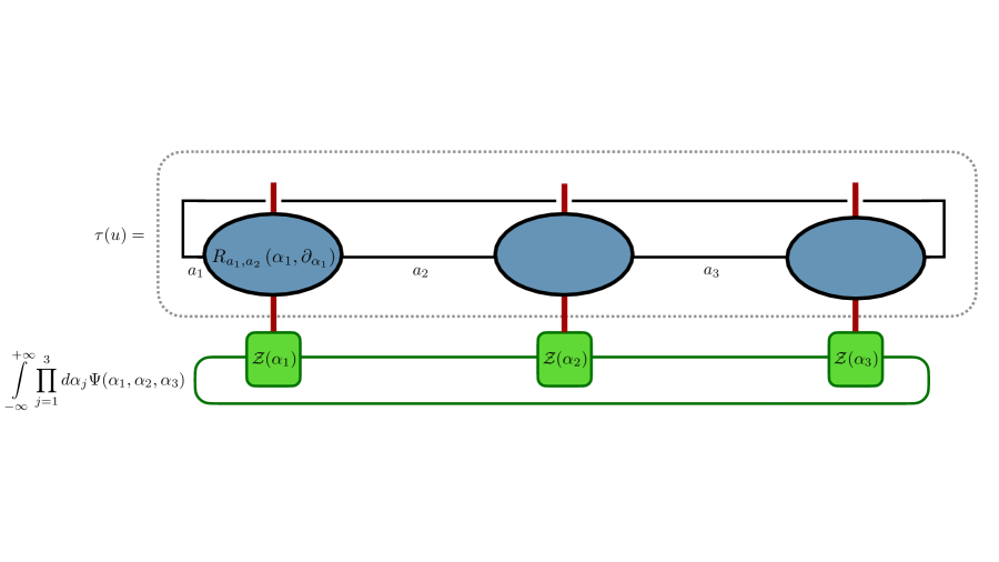
Figure 1: Action (21) for $L=3$. In this case, each $R$-matrix is linear in $u$ so in total $\tau(u)$ is a differential operator in $\alpha_{j},\partial_{\alpha_{j}}$ which is cubic in $u$; in other words, it is a collection of four differential operators, one for each power of $u$. In practice three of these are trivial and one leads to a nice differential equation on the wave function upon integration by parts. This leads to equation (24) coming from the $u^{0}$ term in $\tau(u)$.

From the R-matrix, one can construct the transfer-matrix, which acts on the full light-ray operator through

$$\tau(u)\cdot\text{Tr}\left(\mathcal{Z}(\alpha_{1}z)\dots\mathcal{Z}(\alpha_{L})\right)=\text{Tr}\left(\left(R_{a_{1}a_{2}}Z(\alpha_{1})\right)\dots\left(R_{a_{L}a_{1}}Z(\alpha_{L})\right)\right),$$ (21)

see figure 1 for a graphical description of $R$ and $\tau$. For our purposes, it suffices to know that the transfer matrix commutes with itself and the dilatation operator for any value of the spectral parameter,

$$[\tau(u),\tau(v)]=[\tau(u),\mathbb{D}]=0.$$ (22)

Local single-trace operators are eigenvectors of $\tau(u)$ and therefore so are their light transforms. We demand that this remains true for more general light-ray operators corresponding to the continuation of the light-transforms at non-integer spin:

$$\tau(u)\cdot\mathbb{O}=t(u)\mathbb{O}.$$ (23)

The transfer matrix equation (23) is a polynomial in $u$ of degree $L$. Collecting (23) in powers of $u$ provides a number of differential equations that must be satisfied by $\mathbb{O}$. The differential operators naturally act on the partons through (21). Integrating the action by parts results in a system of differential equations for the wave functions $\Psi$. Ignoring the trivial $u^{L}$ term, this provides a set of $L$ equations on the $L$-variable wavefunction $\Psi$. Note that, after imposing the kinematical constrains, the $u^{L-1}$ and $u^{L-2}$ terms in (23) are redundant, the first being equivalent to (11) and the second equivalent to (12). We are thus left with $L-2$ non-trivial conditions on $\Psi$. For $L=3$, using (18), the nontrivial equation reads

$$\tfrac{1}{2}\left(1+\cos(6\theta)\right)g^{(3)}-\tfrac{3}{2}(4+S)\sin(6\theta)g^{(2)}-\left(\left(3S^{2}+6S+8\right)+\left(3S^{2}+24S+44\right)\cos(6\theta)\right)g^{\prime}$$

$$=(\tfrac{1}{2}(12i\sqrt{3}q+(2+S)(4+S)(6+S)\sin(6\theta)))g,$$ (24)

where $q$ is defined by

$$t(u)=2u^{3}-\tfrac{1}{4}C_{2}(S)u+\tfrac{q}{8},$$ (25)

with $C_{2}(S)=S^{2}+2S+\tfrac{3}{2}$.

The periodicity of (24) invites us to work in Fourier space. The discrete symmetries of $g$, equation (19), imply that, as a distribution,

$$g(\theta)=\sum_{n\in\mathbb{Z}}a_{n}(-1)^{n}e^{i6n\theta},$$ (26)

where we introduced factors of $(-1)^{n}$ for later convenience. Indeed, plugging the decomposition (26) in (24) leads to a beautiful three-term recursion relation! We summarize the results of this section in the following box.

Dynamic Constraints on $\Psi$ ($L=3$) The $g(\theta)$ distribution defining one-loop even-trajectory single-trace light-ray operators through (18) must satisfy $\displaystyle(6n-S)(2+6n-S)(4+6n-S)a_{n+1}$ $\displaystyle-12(n\left(8+36n^{2}+6S+3S^{2}\right)-2\sqrt{3}q)a_{n}$ (27) $\displaystyle+(6n-4+S)(6n-2+S)(6n+S)a_{n-1}=0,$ where $a_{n}$ are the Fourier coefficients of $g(\theta)$ defined in (26) and $q$ is an operator dependent charge defined in (25).

The determination of the light-ray wave functions corresponding to the various presumed discrete trajectories can be separated into two parts. First, one should understand what fixes, for the various discrete trajectories, indexed by $j$, the integrable charge eigenvalue $q_{j}(S)$ at non-integer spin. Second, given $q_{j}(S)$, one must determine how to fix a unique solution to (27). At this point there remains a continuous one parameter family of solutions to (27). We solve these issues in section 2.5. However, first it is useful to consider the case of light transforms of local operators from the perspective of (27).

2.4 Integer spin and reduction to the light transform

For even integer spin $2k$, the ansatz (10, 18) reduces to

$$\mathbb{O}=\int\mathop{}\!\mathrm{d}\alpha_{cm}\mathop{}\!\mathrm{d}\theta\mathop{}\!\mathrm{d}rg(\theta)\delta^{(2k)}(r)\text{Tr}\left(\mathcal{Z}(y+\alpha_{1}z)\mathcal{Z}(y+\alpha_{2}z)\mathcal{Z}(y+\alpha_{3}z)\right)+O(S-2k),$$

where we assumed that $g(\theta)$ is regular as $S=2k$, and the $\alpha_{i}$ are understood to be functions of $\alpha_{cm},r,\theta$ according to (15-17). Because the radial part of the kernel degenerates into a delta function the fields $\mathcal{Z}$ localize,

$$\mathbb{O}=\int\mathop{}\!\mathrm{d}\alpha_{cm}\mathop{}\!\mathrm{d}\theta g(\theta)\sum_{j=0}^{2k}P_{j}(\theta)\text{Tr}\left(\mathcal{Z}(z\cdot D)^{j}\mathcal{Z}(z\cdot D)^{2k-j}\mathcal{Z}\right)(y+\alpha_{cm}z)+O(S-2k),$$ (29)

where $P_{j}$ is a homogeneous polynomial of degree $S$ on sine and cosine of $\theta$. Due to this property of $P_{j}$, the wave function $g(\theta)$ can be truncated in its Fourier decomposition: only $a_{n}$ with $|n|\leq\lfloor\tfrac{S}{6}\rfloor$ can contribute in (29).

Let us now examine the recursion relation (27) for integer spin. Beautifully, for even $S$ the equations indexed by $|n|\leq\lfloor\tfrac{S}{6}\rfloor$ close! Indeed, these equations provide a system of $2\lfloor\tfrac{S}{6}\rfloor+1$ equations on the $2\lfloor\tfrac{S}{6}\rfloor+1$ variables $a_{n}$, $|n|\leq\lfloor\tfrac{S}{6}\rfloor$. A non-trivial solution to these linear equations is possible if and only if the determinant of the matrix of coefficients vanishes. This condition is a polynomial equation of degree $2\lfloor\tfrac{S}{6}\rfloor+1$ for $q$. Each solution to this equation will then define, up to normalization, the light transform of a local operator by means of (29)! Indeed, there are $2\lfloor\tfrac{S}{6}\rfloor+1$ primary twist three operators at even spin $S$. (See appendix A for the counting of local primaries for arbitrary twist $L$ and spin $S$.) We therefore recover the complete spectrum of even-spin twist-three local operators from the light-ray construction, including the integrable charge $q$ characterizing each of them.

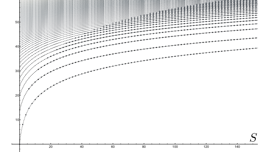
Figure 2: Black dots: even spin twist three spectrum up to $S=150$. Black dashed curves: first $50$ analytic trajectories continuing the even spin spectrum. They correspond to the light-ray operators constructed in section 2. The black lines are constructed entirely from the the physical states using (30). Alternatively, they can be obtained from the action of the light-ray Hamiltonian, see discussion around (34), or directly from integrability, see section 4. One might wonder if there are alternative ways of organizing the spectrum into analytic trajectories. Consider for example the red dashed curve, which is drawn by hand. Is there an analytic trajectory which continues the selected local operators? We expect that the answer is negative, and indeed, under the assumption of analyticity in a half-plane, this can be verified using (30), see appendix 5. However, surprisingly, it turns out that, indeed, there are (infinitely many) other reorganizations of the spectrum into analytic families. We discuss this surprising fact in the conclusions and in appendix 5.

Due to integrability, it is straightforward to compute the CFT data associated to these operators. In figure 2 we present all one-loop anomalous dimension for even spin twist three operators up to spin $S=150$.

The black dashed lines in figure 2 represent a complete set of trajectories ordered by their anomalous dimensions. It is possible to provide a numerical argument that this assignment of local operators into families indeed corresponds to analytic Regge trajectories. Assuming no mixing of trajectories in a half right plane, the complex spin CFT data associated to a given Regge trajectory admits a convergent expansion in terms of the integer spin CFT data through a Newton series [13]. For instance, in the case of the anomalous dimension $\gamma(S)$ we have

$$\gamma(S)=\sum_{n=0}^{\infty}\binom{\tfrac{S-S_{0}}{2}}{n}\sum_{i=0}^{n}(-1)^{n-i}\binom{n}{i}\gamma_{S_{0}+2i},$$ (30)

where $\gamma_{S}$ corresponds to the integer spin CFT data. Convergence is guaranteed to the right of the first singularity in the complex spin plane. In (30), we are free to choose $S_{0}$ to be any integer along the trajectory — $\gamma(S)$ should be insensitive to this choice for a consistent Regge trajectory. One can then use the self-consistency of equation (30) to probe whether a given assignment of local operators into trajectories is consistent with analyticity in spin.

Plugging the anomalous dimension associated to the integer spin operators of the black trajectories in figure 2 indeed results in beautiful numerical convergence of (30). Indeed, the black curves themselves are generated through Newton’s formula, and can be double checked against other methods, see [13]. On the other hand, alternative assignments of local operators to trajectories, such as the red curves in figure 2, result in numerical divergences via (30) — see section 5. This suggests that such assignments do not correspond to Regge trajectories controlling CFT correlators.

Newton’s series can also be used to reconstruct the analytic continuation of the integrable charge $q_{j}(S)$ associated to the various black trajectories, indexed henceforth by $j$, from the integer spin $q$ values obtained from (27). The problem of determining the values of $q_{j}(S)$ for non-integer spin is thus in practice solved, at least in a half-plane. In this work, however, we would like to understand how the black trajectories and $q_{j}(S)$ are selected from the point of view of light-ray operators, i.e. directly from (27) at non-integer spin.

2.5 Quantization at non-integer spin

Light-ray operators at non-integer spin should diagonalize the one-loop dilatation operator, which acts by

$$\mathbb{D}_{1}\cdot\text{Tr}\left(\mathcal{Z}(\alpha_{1})\dots\mathcal{Z}(\alpha_{L})\right)=\sum_{i=1}^{L}\mathcal{H}_{i,{i+1}}\cdot\text{Tr}\left(\mathcal{Z}(\alpha_{1})\dots\mathcal{Z}(\alpha_{L})\right),$$ (31)

$$\mathcal{H}_{i,{i+1}}\cdot\text{Tr}\left(\mathcal{Z}(\alpha_{1})\dots\mathcal{Z}(\alpha_{L})\right)=2g^{2}\int\frac{\mathop{}\!\mathrm{d}\tau}{\tau}\Big{(}2\text{Tr}\left(\dots\mathcal{Z}(\alpha_{i})\mathcal{Z}(\alpha_{i+1})\dots\right)$$

$$-\text{Tr}\left(\dots\mathcal{Z}((1-\tau)\alpha_{i}+\tau\alpha_{i+1})\mathcal{Z}(\alpha_{i+1})\dots\right)-\text{Tr}\left(\dots\mathcal{Z}(\alpha_{i})\mathcal{Z}((1-\tau)\alpha_{i+1}+\tau\alpha_{i})\dots\right)\Big{)},$$

where $\mathcal{Z}(\alpha)\equiv\mathcal{Z}(\alpha n^{+})$. Demanding that $\mathbb{O}$ diagonalize $\mathbb{D}_{1}$ implies an integral equation for the light-ray wavefunction $\Psi$. In the study of the Wilson-Fisher theory in [14], an analogous integral equation implied certain smoothness/boundary conditions for $\Psi$, leading to quantization conditions and discrete solutions.

Here, instead of analyzing how smoothness/boundary conditions come about from (31), we will instead guess a simple quantization condition using our Fourier-space recursion relation, and then check its consistency with $\mathbb{D}_{1}$. It is natural to expect that the quantization condition is associated to analyticity properties of $g(\theta)$. We are thus led to examine the asymptotics of the Fourier coefficients $a_{n}$.

Let us consider the large $|n|$ asymptotics of (27) and look for power series solutions. The most general asymptotic solution takes the form

$$a_{n}=\alpha_{1}n^{-1}\left(1+\sum_{i=1}^{\infty}a_{i}n^{-i}\right)+\alpha_{2}n^{S}\left(1+\sum_{i=1}^{\infty}b_{i}n^{-i}\right),$$ (32)

with $a_{i}$, $b_{i}$ fixed in terms of $q$ and $S$ through the recursion relation. Let us emphasize that the asymptotic behaviors at $n\rightarrow\pm\infty$ are in principle distinct. Both should take the form (32), but with different values of $\alpha_{i}$. Let us denote those by $\alpha_{i}(\pm\infty)$ respectively. It is a non-trivial connection problem to determine $\alpha_{i}(-\infty)$ given the $\alpha_{i}(+\infty)$ asymptotics, $q$ and $S$.

This connection problem can be explored numerically. Truncating the sums in (32) with a decent number of terms provides a good approximation to a solution of (27) at large positive values of $n$. From there, one can reconstruct the solution for arbitrary $n$ through iterations of the recursion relation (27). In this way, one can numerically fit $\alpha_{i}(-\infty)$ as a function of $q$, $S$, and $\alpha_{i}(+\infty)$.

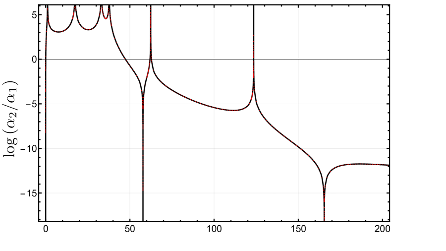
Figure 3: We consider solutions of the recursion relation (27) that decay as $n^{-1}$ for $n\rightarrow+\infty$. The recursion relation then determines the asymptotics as $n\rightarrow-\infty$ to be of the form (32) with $\alpha_{2}/\alpha_{1}$ fixed in terms of $S$ and $q$. Here we plot the ratio as a function of $q$ for $S=6+1/3$. Zeroes of the ratio correspond to values of $q$ for which solutions with pure $|n|^{-1}$ asymptotic exist. Our main proposal is that these are precisely the light-ray operators corresponding to Regge trajectories, see (33).

In figure 3 we plot the ratio ${\alpha_{2}(-\infty)}/{\alpha_{1}(-\infty)}$ as a function of $q$ for the solution of (27) with $\alpha_{2}(+\infty)=0$. We fix the spin $S=6+1/3$, just for the purposes of illustration. Zeroes of the ratio correspond to discrete values $q_{j}(S)$ for which solutions with pure $|n|^{-1}$ asymptotics — and thus maximal smoothness in $\theta$ space — exist. The result is remarkable: these discrete values correspond precisely to the values $q_{j}(S)$ determined by the black trajectories in figure 2! We are thus led to the following proposal.

Quantization Condition on $\Psi$ ($L=3$) The solutions of (27) corresponding to light-ray operators governing Regge trajectories, equivalent to the black curves in figure 2, are those for which asymptotically $$a_{n}\sim|n|^{-1}.$$ (33) At fixed $S$, these exist only for discrete values $q_{j}$ of the integrable charge. These define the infinitely many discrete twist three trajectories as a function of spin.

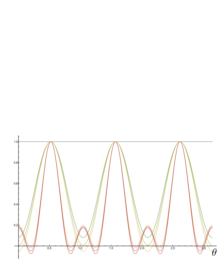
Figure 4: Top: The dynamical part of the wave function, $g(\theta)$, for the lowest even-spin trajectory at various values of spin. From red to green, spin is taken from $S=-1-1/3$ to $S=6-1/3$ in unit steps. The wave function has logarithmic divergences when partons collide. We see three such divergencies in the plot, which correspond respectively to $\alpha_{2}=\alpha_{3}$, $\alpha_{1}=\alpha_{2}$, and $\alpha_{3}=\alpha_{1}$. Bottom: At integer spin, it is enough to truncate the wave function to the first few Fourier modes in order to recover the light-transform of local operators, see section 2.4. From green to red, the lowest trajectory at even spin from $S=4$ to $S=16$.

To test the proposal (33) we can check the action of the one-loop dilatation operator (31) on the corresponding light-ray operators. In practice, we compute

$$\tilde{\gamma}\equiv\frac{\langle\Omega|{\rm Tr}\left(\bar{\mathcal{X}}^{2}\bar{\mathcal{Z}}\right)(x_{1})\left[\mathbb{D}_{1},\mathbb{O}(x_{2})\right]{\rm Tr}\left({\mathcal{X}}\bar{\mathcal{Z}}\right)(x_{3}){\rm Tr}\left({\mathcal{X}}\bar{\mathcal{Z}}\right)(x_{4})|\Omega\rangle}{\langle\Omega|{\rm Tr}\left(\bar{\mathcal{X}}^{2}\bar{\mathcal{Z}}\right)(x_{1})\mathbb{O}(x_{2}){\rm Tr}\left({\mathcal{X}}\bar{\mathcal{Z}}\right)(x_{3}){\rm Tr}\left({\mathcal{X}}\bar{\mathcal{Z}}\right)(x_{4})|\Omega\rangle}$$ (34)

for a range of cross ratios $z,\bar{z}$. We observe that solutions defined through the criteria (33) indeed correspond to cross-ratio independent $\tilde{\gamma}$, as it must be for light-rays diagonalizing $\mathbb{D}_{1}$. Solutions of (27) with alternative asymptotics do not pass this consistency check, $\tilde{\gamma}$ being a non-trivial function of the cross-ratio in those cases. Moreover, for the solutions defined by (33), we observe that $\tilde{\gamma}$ agrees with $\gamma(S)$, as determined by Newton series, for each of the black trajectories in figure 2.

We have thus completed the explicit construction of the operators analytically continuing the (light transform of) even spin triple-twist single-trace operators. They are given by (10) with $\Psi$ given by (18) in terms of $g(\theta)$, which in turn is fixed by (27) and (33). We can explicitly plot these kernels, see figure 4.

3 Norm and structure constants

With explicit light-ray operators in hand, we can compute any correlator we want. Our next task is to relate correlators of light-ray operators to the analytic continuation of local CFT data. This will allow us to understand the origin of the decoupling zeroes in [13]. Local CFT data is usually presented in conventions where local two-point functions have a standard normalization. Thus, in order to relate correlators of light-ray operators to this data, we must understand how to properly define the norm of light-ray operators.

This is not totally straightforward: light-ray operators annihilate the vaccuum [12]

$$\mathbb{O}(X,Z)|\Omega\rangle=0$$ (37)

and therefore Wightman two-point functions do not define a proper norm for these continuous spin operators.

A natural suggestion is, instead, to capture the light-rays norms through their time ordered correlators, as suggested in [15]. One could thus hope for a formula of the form

$$C_{\mathcal{O}_{S}O_{1}O_{2}}^{2}(S)\stackrel{{\scriptstyle?}}{{=}}f_{\mathcal{O}_{S}O_{1}O_{2}}(S)\left(\frac{\langle\mathcal{O}_{1}\mathbb{O}\mathcal{O}_{2}\rangle}{\langle 0|\mathcal{O}_{1}\mathbb{O}\mathcal{O}_{2}|0\rangle}\right)^{2}\frac{\langle 0|\mathbb{O}\bar{\mathbb{O}}|0\rangle}{\langle\mathcal{T}\{\mathbb{O}\bar{\mathbb{O}}\}\rangle},$$ (38)

where $f_{\mathcal{O}_{S}O_{1}O_{2}}(S)$ is some universal function depending exclusively on the various conformal quantum numbers of the operators, $\langle 0|\mathcal{O}_{1}\mathbb{O}\mathcal{O}_{2}|0\rangle$ and $\langle 0|\mathbb{O}\bar{\mathbb{O}}|0\rangle$ are canonical conformal two- and three-point structures defined in appendix B, and $\langle\mathcal{O}_{1}\mathbb{O}\mathcal{O}_{2}\rangle$, $\langle\mathcal{T}\{\mathbb{O}\bar{\mathbb{O}}\}\rangle$ are the dynamical correlators. Let us stress that, out of the various factors in equation (38), only $\langle\mathcal{O}_{1}\mathbb{O}\mathcal{O}_{2}\rangle^{2}/\langle\mathcal{T}\{\mathbb{O}\bar{\mathbb{O}}\}\rangle$ is dynamical and theory dependant, all other factors are kinematical.

The definition of a “time-ordered” correlator of light-ray operators is somewhat subtle. In a perturbative CFT, we will define it by starting with a time-ordered correlator of the constituent fields that make up the light-ray operator, and then integrating against the appropriate kernel $\Psi$. In a nonperturbative CFT, one approach is to construct the light-ray operator via a bilocal integral of local operators [12], and apply the bilocal kernel to a time-ordered correlator (as in the derivation of [14]). The relationship between these approaches is not obvious. Fortunately, the simple perturbative definition will be suitable for this work.

3.1 (Twist 2 motivation of the) complex $S$ structure constant formula

To get some intuition on how the formula (38) might work, let us consider the case of twist two light-ray operators,

$$\!\!\!\!\!\!\!\!\mathbb{O}_{2}=\frac{i\sqrt{2}\sqrt{\Gamma(2S+1)}}{2\pi\Gamma(S+1)}\!\!\int\limits_{-\infty}^{\infty}\!\!d\alpha_{1}d\alpha_{2}{\underbrace{\left(\frac{1}{(\alpha_{1}-\alpha_{2}+i\epsilon)^{1+S}}+\frac{1}{(\alpha_{2}-\alpha_{1}+i\epsilon)^{1+S}}\right)}_{\psi(\alpha_{1},\alpha_{2})}}\text{Tr}\left(\mathcal{Z}(y+\alpha_{1}z)\mathcal{Z}(x+\alpha_{2}z)\right)$$ (39)

at leading order. The full computation is completely fixed by conformal symmetry in this case, and thus we can explicitly keep track of all factors contributing to (38). We will take $O_{1}={\rm Tr}\left(\mathcal{X}\bar{\mathcal{Z}}\right)$ and $O_{2}={\rm Tr}\left(\bar{\mathcal{X}}\bar{\mathcal{Z}}\right)$ in this example.

At even integer spin, these light-rays reduce to light-transforms of local twist-2 operators,

$$\phantom{}\qquad\mathbb{O}_{S}(x,z)=L[\mathcal{O_{S}}](x,z)\qquad\text{for even integer $S$,}$$

where

$$\mathcal{O}_{S}(x,z)=\frac{1}{\sqrt{2(2S)!}}\sum_{i}(-1)^{i}\binom{S}{i}^{2}\text{Tr}\left(D^{i}_{z}\mathcal{Z}D^{S-i}_{z}\mathcal{Z}\right)(x).$$

The operators $\mathcal{O}_{S}$ are canonically normalized,

$$\langle\mathcal{O}(x_{1},z_{1})\mathcal{O}(x_{2},z_{2})\rangle=\frac{\left((x_{12}\cdot z_{1})(x_{12}\cdot z_{2})-\tfrac{1}{2}x_{12}^{2}(z_{1}\cdot z_{2})\right)^{S}}{(x_{12}^{2})^{\Delta+S}},$$ (40)

and the three point function of interest is

$$\langle\mathcal{O}_{1}(x_{1})\mathcal{O}_{S}(x_{3},z)\mathcal{O}_{2}(x_{2})\rangle=\frac{\sqrt{2}S!}{\sqrt{2S!}}\frac{\left(z\cdot x_{23}x_{13}^{2}-z\cdot x_{13}x_{23}^{2}\right)^{S}}{x_{23}^{\Delta+S}x_{13}^{\Delta+S}x_{12}^{2}},$$ (41)

from which one can read that $C_{\mathcal{O}_{S}O_{1}O_{2}}(S)=\sqrt{2}\Gamma(S+1)/\sqrt{\Gamma(2S+1)}$.

Let us reproduce this result directly at complex spin from $\langle\mathcal{O}_{1}\mathbb{O}\mathcal{O}_{2}\rangle$ and $\langle\mathcal{T}\{\mathbb{O}\bar{\mathbb{O}}\}\rangle$. At leading order these correlators are given by simple Wick contractions. The computation is discussed briefly in figure 5. Details and further discussion can be found in appendix B.

The computation of $\langle\mathcal{O}_{1}\mathbb{O}\mathcal{O}_{2}\rangle$ is straightforward. One simply deforms the $\alpha_{i}$ integrals and picks up the propagator poles. The result is

$$\frac{\langle\mathcal{O}_{1}(x_{1})\mathbb{O}\mathcal{O}_{2}(x_{2})\rangle}{\langle 0|\mathcal{O}_{1}\mathbb{O}\mathcal{O}_{2}|0\rangle}=\left(-2\pi i\frac{\Gamma(2S+1)}{\Gamma(S+1)^{2}}\right)C_{\mathcal{O}_{S}O_{1}O_{2}}(S).$$ (42)

The term in parenthesis can be understood as resulting from the light-transform of the canonical three-point structure [12]. Indeed, now restoring explicit dependence on the twist $\tau=\Delta-J$ and allowing for generic dimensions $\Delta_{1},\Delta_{2}$ for the scalar operators $\mathcal{O}_{1}$ and $\mathcal{O}_{2}$, we have

$$\int dx_{3}^{+}\frac{(x_{2}^{-}x_{13}^{2}-x_{1}^{-}x_{23}^{2})^{S}}{x_{23}^{\tau+2S+\Delta_{2}-\Delta_{1}}x_{13}^{\tau+2S+\Delta_{1}-\Delta_{2}}x_{12}^{\Delta_{1}+\Delta_{2}-\tau}}=$$ (43)

$$\left(\frac{-2\pi i\Gamma(\tau+2S-1)}{\Gamma(\tfrac{\tau+\Delta_{1}-\Delta_{2}+2S}{2})\Gamma(\tfrac{\tau+\Delta_{2}-\Delta_{1}+2S}{2})}\right)\frac{\left(\tfrac{x_{1}^{2}}{x_{1}^{-}}-\tfrac{x_{2}^{2}}{x_{2}^{-}}\right)^{1-\tau-S}}{x_{12}^{\Delta_{1}+\Delta_{2}-\tau}(x_{1}^{-})^{(\Delta_{1}-\Delta_{2}+\tau)/2}(-x_{2}^{-})^{(\Delta_{2}-\Delta_{1}+\tau)/2}}.$$

The second term above is our definition for the kinematical three point conformal structure $\langle 0|\mathcal{O}_{1}(x_{1})\mathbb{O}(-\infty n^{+},n^{+})\mathcal{O}_{2}(x_{2})|0\rangle$. The numerical prefactor in parenthesis will be absorbed as part of $f_{\mathcal{O}_{S}O_{1}O_{2}}(S)$ in (38).

Figure 5: Structure constants between the non-local operator and two local scalar operator are obtained by Wick contracting the constituents of the line operator with the scalars (left) as well as normalizing the light-ray operator by dividing by its norm (right). Here we are considering the twist two case where two partons are integrated along a light-ray. The left picture yields (42) while the right picture leads to (45).

Next we move on to the computation of $\langle\mathcal{T}\{\mathbb{O}(x_{1},z_{1})\bar{\mathbb{O}}(x_{2},z_{2})\}\rangle$. The computation is immediately more subtle. The correlator is invariant under the action of a $SO(1,1)$ conformal transformation — the $M_{+-}$ boost in the frame of figure 5. Its action on the fields of (39) can be absorbed by rescaling the integration variables.

One thus has a zero-mode in the integrals. It produces a divergent factor $\text{vol}(SO(1,1))$ upon integration. We will divide the correlator by this factor to obtain a finite result. In practice, this means ‘gauge fixing’ the action of the $M_{+-}$ boost and inserting the proper Faddeev-Popov determinant, which guarantees the result is gauge independent.

We thus want to compute

$$\langle\mathcal{T}\{\mathbb{O}\bar{\mathbb{O}}\}\rangle_{\text{g.f.}}=\frac{\Gamma(2S+1)}{4\pi^{2}\Gamma(S+1)^{2}}\int\prod_{i=1}^{2}d\alpha_{i}d\beta_{i}\frac{\lambda\delta(\alpha_{1}+\alpha_{2}-\lambda)\psi(\alpha_{1},\alpha_{2})\psi(\beta_{1},\beta_{2})}{(\alpha_{1}\beta_{1}+d^{2}+i\epsilon)(\alpha_{2}\beta_{2}+d^{2}+i\epsilon)},$$ (44)

where we inserted the gauge fixing (g.f.) condition $\alpha_{1}+\alpha_{2}=\lambda$, with the overall factor of $\lambda$ being the Faddeev-Popov determinant ensuring that the result is independent of $\lambda$. As in the three-point element computation, there are two possible Wick contractions which can be combined into a factor of two by permutation symmetry of the wave function $\psi(\beta_{1},\beta_{2})$.

The computation is performed in appendix B. The result is

$$\frac{\langle\mathcal{T}\{\mathbb{O}\bar{\mathbb{O}}\}\rangle_{\text{g.f.}}}{\langle 0|\mathbb{O}\bar{\mathbb{O}}|0\rangle}=-\frac{\left(1+e^{i\pi(-1-S)}\right)}{(2S+1)}.$$ (45)

Combining the results (42) and (45) allows us to write a sharp version of (38):

Continuation of Structure Constants from Light-Ray Correlators The analytic continuation in spin of structure constants is given in terms of light-ray correlators as $$C_{\mathcal{O}_{S}O_{1}O_{2}}^{2}(S)=f_{\mathcal{O}_{S}O_{1}O_{2}}(S)\left(\frac{\langle\mathcal{O}_{1}\mathbb{O}\mathcal{O}_{2}\rangle}{\langle 0|\mathcal{O}_{1}\mathbb{O}\mathcal{O}_{2}|0\rangle}\right)^{2}\frac{\langle 0|\mathbb{O}\bar{\mathbb{O}}|0\rangle}{\langle\mathcal{T}\{\mathbb{O}\bar{\mathbb{O}}\}\rangle_{\text{g.f.}}}$$ (46) with $$f_{\mathcal{O}_{S}O_{1}O_{2}}(S)\equiv\frac{e^{-i\pi S}-1}{\Delta+S-1}\left(\frac{\Gamma\left(\tfrac{\tau+\Delta_{1}-\Delta_{2}+2S}{2}\right)\Gamma\left(\tfrac{\tau+\Delta_{2}-\Delta_{1}+2S}{2}\right)}{2\pi i\Gamma(\tau+2S-1)}\right)^{2}$$ (47) where $\langle 0|\mathcal{O}_{1}\mathbb{O}\mathcal{O}_{2}|0\rangle$ and $\langle 0|\mathbb{O}\bar{\mathbb{O}}|0\rangle$ are canonical two- and three-point structures defined by the quantum numbers of the various operators, $\langle\mathcal{O}_{1}\mathbb{O}\mathcal{O}_{2}\rangle$ is the three-point correlator and $\langle\mathcal{T}\{\mathbb{O}\bar{\mathbb{O}}\}\rangle_{\text{g.f.}}$ is the light-ray norm as defined above.

We have derived this formula only in the case of twist two light-rays at leading order, so from this perspective (46) is an ansatz. In the next section, we will use this formula to compute structure constants for the various twist three light-ray operators constructed in section (2) at complex spin. We can then compare — at least in the right-half spin plane — the results obtained with (46) to the complex spin structure constants obtained using Newton’s formula in [13] — see the analogous (30) for anomalous dimensions. The match is perfect. Given that the twist three light-rays are certainly not fixed by conformal symmetry and depend in detail on the dynamics of the theory, this gives robust evidence that (46) is correct in general. This was our route to argue for (46). As mentioned in footnote 16, a direct non-perturbative argument is given in [14].

3.2 Structure constants at twist 3 from light-ray wave functions

The integrals computing twist two structure constants, being controlled by conformal symmetry, could be done analytically. For twist three, the dynamical correlators $\langle\mathcal{O}_{1}\mathbb{O}_{n,S}\mathcal{O}_{2}\rangle$ and ${\langle\mathcal{T}\{\mathbb{O}_{n,S}\bar{\mathbb{O}}_{n,S}\}\rangle}$ are given by non-trivial integrals over the dynamical part of the twist three wave functions: the functions $g(\theta)$ fixed by the quantization condition (33). The computation is discussed in figure 6 and the precise expressions are derived in appendix B. In this section, we quote the results and discuss the evaluation of the twist three structure constants directly from the light-rays constructed in section 2. This will enable us to discuss the origin of the decoupling zeroes uncovered in [13] from the light-rays.

We parametrize twist three light-rays inserted at $x=-\infty n^{+}$, $z=n^{+}$ as

$$\mathbb{O}_{n,S}=\int d\alpha_{\text{cm}}drd\theta\left(\psi\left(\alpha_{cm},r,\theta\right)\equiv\frac{1}{\Gamma(S_{n}^{*}-S)}\frac{g_{n,S}(\theta)}{r^{1+S}}\right)\text{Tr}\left(\mathcal{Z}(\alpha_{1})\mathcal{Z}(\alpha_{2})\mathcal{Z}(\alpha_{3})\right),$$ (48)

with $\alpha_{i}$ being parametrized by $(\alpha_{cm},r,\theta)$ according to (15-17) as

$$\alpha_{i} =\alpha_{cm}+\tfrac{1}{3}r\alpha_{i}^{\theta},$$ (49)

$$\alpha_{i}^{\theta} =\cos(\theta-2\pi(i-1)/3)-\cos(\theta-2\pi(i-2)/3).$$ (50)

We introduce the $\Gamma$ function factor for later convenience, where $S_{n}^{*}=6(n-1)$ is the first integer spin in which the $n$-th even trajectory has physical operators, see figure 2.

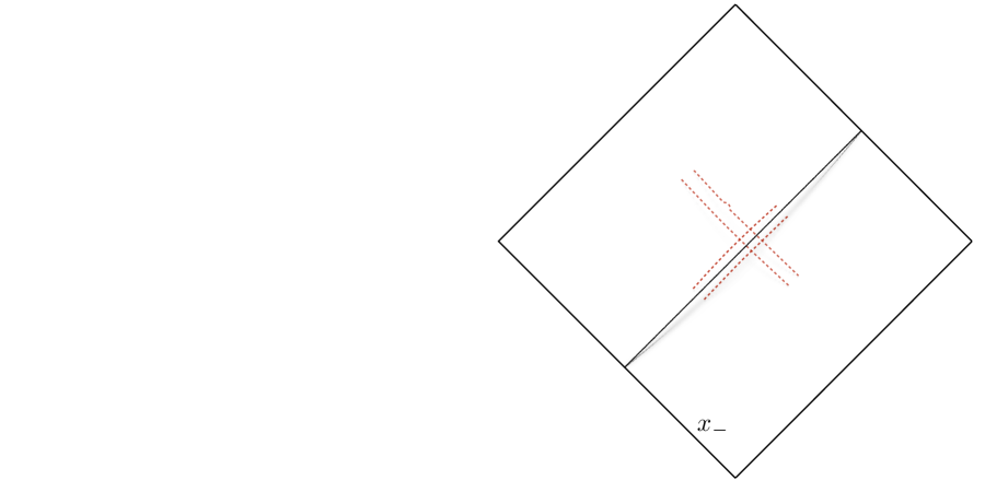
Figure 6: Same as figure 5 but for twist three operators, made of three partons. The left picture leads to (51) – once two of the three parton integrations is carried out explicitly – while the right picture yields (52) – once we take care of three of the six integrations depicted in the figure.

The computation of the matrix elements $\langle\mathcal{O}_{1}\mathbb{O}_{n,S}\mathcal{O}_{2}\rangle$ is straightforward. The triple integral is reduced to a single integral by deforming two of the integral contours, picking up propagator poles. The result is

$$\frac{\langle\mathcal{O}_{1}\mathbb{O}\mathcal{O}_{2}\rangle}{\langle 0|\mathcal{O}_{1}\mathbb{O}\mathcal{O}_{2}|0\rangle}=\frac{1}{\sin(\pi S)\Gamma(S^{*}_{n}-S)}\int d\theta g(\theta)F_{\text{three points}}(\theta),$$ (51)

which must be evaluated numerically for each trajectory as we will discuss later. The kernel $F_{\text{three points}}$ is purely kinematical, and is defined in equation (108).

As in the twist two case, the twist three norm $\langle\mathcal{T}\{\mathbb{O}\bar{\mathbb{O}}\}\rangle$ requires gauge fixing. We use the gauge $\delta(r_{\alpha}-1)$. The starting point is given by a six-dimensional integral. Two integrals can be performed by residues, while one is localized by the delta function, see appendix B. The result is

$$\frac{\langle\mathcal{T}\{\mathbb{O}\bar{\mathbb{O}}\}\rangle_{\text{g.f.}}}{\langle 0|\mathbb{O}\bar{\mathbb{O}}|0\rangle}=\frac{1}{\sin(\pi S)\Gamma(S_{n}^{*}-S)^{2}}\int_{D}d\alpha_{cm}d\theta_{\alpha}d\theta_{\beta}g_{\mathbb{O}}(\theta_{\alpha})g_{\bar{\mathbb{O}}}(\theta_{\beta})F_{\text{two point}}(\alpha_{cm},\theta_{\alpha},\theta_{\beta}),$$ (52)

where the kinematical kernel $F_{\text{two point}}$ is defined in (109). The integral over $\alpha_{cm}$ can be performed analytically. Instead, it is enough for our purposes to proceed numerically from this point.

All ingredients necessary to compute the structure constants $C_{\mathbb{O}_{n,S}\mathcal{O}_{1}\mathcal{O}_{2}}$ are now in place.

1. We generate the complex spin wave functions for the various discrete trajectories following section 2. The wave function $g(\theta)$ is approximated by its Fourier series truncated to some large Fourier mode.

2. The integrals (107) and (109) are then evaluated numerically. The multidimensional integral can be straightforwardly computed through Quasi-Monte Carlo.

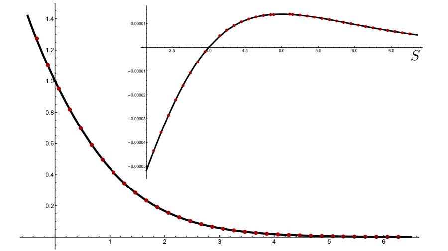
Figure 7: In red, structure constants computed from explicit light-ray operators using (46). In black, the Newton interpolation (30) for the structure constants, see [13]. They match perfectly. We plot the results for the first and second trajectory, including the first decoupling zero.

The result of this computation is shown in figure 7. There is a perfect match with the result obtained from Newton’s formula (30). In particular, the decoupling zeroes of [13] are reproduced.

It is interesting to understand how these decoupling zeroes arise from the point of view of (46). It is important to clarify that the answer to such a question depends on how one normalizes the operators. We chose to normalize the operators $\mathbb{O}_{n,S}$ through the condition $\alpha_{m}=\tfrac{1}{m}+O(\frac{1}{m^{2}})$ for all values of $S$. In this case what happens to the light-ray operators as one approaches a positive even spin value $2k$ is:

• For $S\rightarrow 2k$ with $2k<6(n-1)$, the Fourier modes $a_{m}$ with $|m|\leq\lfloor 2k/6\rfloor$ vanish linearly as $(S-2k)$, other modes remaining finite and non-zero. For $S\rightarrow 2k$ with $2k\geq 6(n-1)$, all Fourier modes $a_{m}$ remain finite and non-zero. We introduce $S_{n}^{*}\equiv 6(n-1)$ for this important threshold value separating these two behaviors.

• Meanwhile, the radial part of the wave function develops a simple pole for $S\rightarrow 2k$ with $2k<S_{n}^{*}$,

  $$\frac{r^{-1-S}}{\Gamma(S_{n}^{*}-S)}=-\frac{\delta^{2k}(r)}{\Gamma(S_{n}^{*}-2k)\Gamma(2k+1)(S-2k)}+O\left((S-2k)^{0}\right)$$ (53)

  and remains finite for $2k\geq S_{n}^{*}$:

  $$\frac{r^{-1-S}}{\Gamma(S_{n}^{*}-S)}=\frac{\Gamma(2k-S_{n}^{*}+1)\delta^{2k}(r)}{\Gamma(2k+1)}+O\left(S-2k\right).$$ (54)

Thus, with this choice of normalization, we see that, for any even integer $2k$, the light-ray operators and their matrix elements such as $\langle\mathcal{O}_{1}\mathbb{O}_{n,S}\mathcal{O}_{2}\rangle$ remain finite and generically non-zero.

When analyzing $\langle\mathcal{T}\{\mathbb{O}\bar{\mathbb{O}}\}\rangle_{\text{g.f.}}$ one needs to be more careful. The presence of the gauge-fixing factor $\delta(r_{\alpha}-1)$ in $\langle\mathcal{T}\{\mathbb{O}\bar{\mathbb{O}}\}\rangle_{\text{g.f.}}$ effectively means we should replace $r_{\alpha}^{-1-S}\rightarrow 1$ in the $\psi_{\mathbb{O}}(\alpha_{i})$ wave function contributing to the light-ray norm. The absence of the $r_{\alpha}^{-1-S}$ factor, which previously produced a pole and a delta function has two effective consequences: first, the light-ray no longer localizes to the first few fourier modes and, second, there is no longer a pole from the distributional limit of $r^{-1-S}$ at even $S$. Thus the radial part for the gauge-fixed operator contributes an extra zero relative to (53) and (54), while the angular part no longer contributes a zero for $2k<S_{n}^{*}$. In total, we conclude that $\langle\mathcal{T}\{\mathbb{O}\bar{\mathbb{O}}\}\rangle_{\text{g.f.}}$ vanishes for $2k\geq S_{n}^{*}$ and remains finite for $2k<S_{n}^{*}$.

Thus in this normalization the decoupling zeroes simply follow from $1-e^{-i\pi S}$ factor in the conversion factor (47). More precisely, for even spin $S=2k\geq S_{n}^{*}$ in which local operators do exist, the conversion factor zero cancels with the zero from the light-ray norm, resulting in a non-zero structure constant. For even spins $S=2k<S_{n}^{*}$ when the local operators do not exist the conversion factor zero has no pole to cancel with and we get a decoupling zero for the structure constant. We summarize the various factors in the following table.

	$\langle\mathcal{O}_{1}\mathbb{O}_{n,S}\mathcal{O}_{2}\rangle$	$\left(\langle\mathcal{T}\{\mathbb{O}\bar{\mathbb{O}}\}\rangle_{\text{g.f.}}\right)^{-1}$	$f_{\mathcal{O}_{S}\mathcal{O}_{1}\mathcal{O}_{2}}(S)$	$C_{\mathcal{O}_{S}O_{1}O_{2}}^{2}(S)$
$2k<S_{n}^{*}$	$(S-2k)^{0}$	$(S-2k)^{0}$	$(S-2k)$	$(S-2k)$
$2k\geq S_{n}^{*}$	$(S-2k)^{0}$	$(S-2k)^{-1}$	$(S-2k)$	$(S-2k)^{0}$

Of course, one could chose to normalize the operators so that

$$f_{\mathcal{O}_{S}\mathcal{O}_{1}\mathcal{O}_{2}}(S)\frac{\langle 0|\mathbb{O}\bar{\mathbb{O}}|0\rangle}{\langle\mathcal{T}\{\mathbb{O}\bar{\mathbb{O}}\}\rangle_{\text{g.f.}}}=1$$

in analogy to what is conventionally done for local operators. In this case, the decoupling zeroes would come directly from the three point correlators $\langle\mathcal{O}_{1}\mathbb{O}_{n,S}\mathcal{O}_{2}\rangle$. Both options are fine.

This was the right-half plane story from the point of view of operators. It is time to see what dragons await us in the left-half plane.

4 The complex plane

4.1 Riemann surface, expectation and result

A main point of this paper so far has been that the various twist three operators organize themselves into infinitely many well defined Regge trajectories. They could be numbered and ordered according to their anomalous dimensions $\gamma_{j}$, or their $q_{j}$ integrable charges, continuously in spin. This picture is correct for the right-half spin plane, where local operators live and where life is plain and simple.

The global picture is quite different: all these various well-defined trajectories merge into a single analytic entity, connected through infinitely many branch points at (seemingly) generic locations in the left half spin plane, see figures 8 and 9. Perhaps surprisingly, this happens in perturbation theory! This is in contrast to more familiar operator mixing such as the well studied BFKL-DGLAP-Shadow mixing [6, 7, 8, 9, 10, 11, 5], for which branch points can only be accessed at finite coupling. In perturbation theory the BFKL-DGLAP cuts close, and manifest as poles at negative integer values of spin. Here instead we consider a infinite number of trajectories which are degenerate in perturbation theory, and thus mix right away, allowing us to explore their rich and complicated Riemann surface already at leading order.

An integrabilist could have foreseen this by examining the local operator data. For example, at spin $S=12$ there are three local operators whose structure constants $C_{n,S}\equiv C_{\mathcal{O}_{n,S}\mathcal{O}_{1}\mathcal{O}_{2}}^{2}$ are given by

$$C_{1,12}^{2} =\frac{11}{12086676},$$

$$C_{2,12}^{2} =\frac{206}{16034270715}+\frac{695219}{(80171353575\sqrt{455745})},$$

$$C_{3,12}^{2} =\frac{206}{16034270715}-\frac{695219}{(80171353575\sqrt{455745})}.$$

with a similar multi-square-root structure being present at higher values of spin. These strongly suggest the various families (with the exception of the lowest trajectory which remains rational at all value of spin) can be analytically continued into each other.

In section 4.2 we will describe how to reconstruct the twist three Riemann surface numerically using integrability methods. The results are described in figures 8 and 9. In section 4.3 we discuss an alternative strategy from which one could in principle reconstruct the Riemann surface from the local operator spectrum.

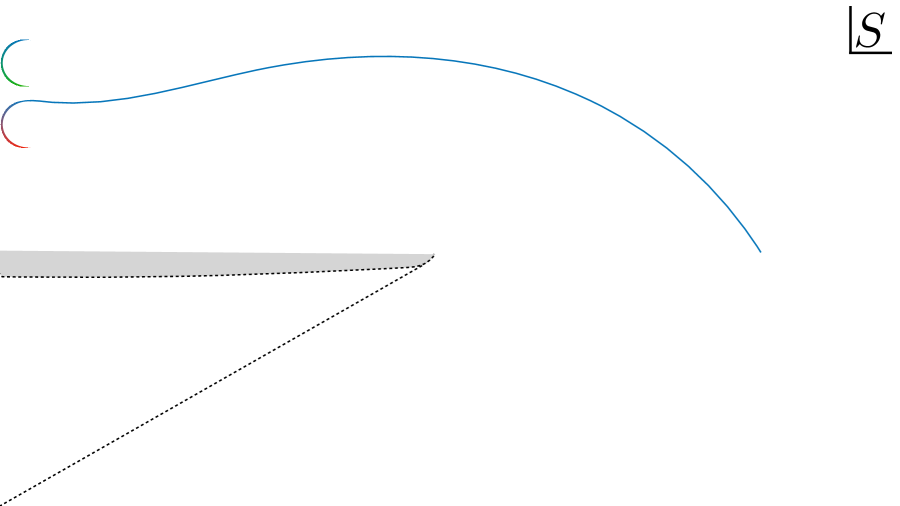
Figure 8: Here we present the analytic continuation of the various operators to the left half-plane. We observe no interesting structure to the right of a dashed cone, which includes the positive integers where the light-rays reduce to light-transforms of local operators, and where we observe the decoupling zeroes discussed in section 3. If we start with a certain family on the right, go for a walk on the left and come back to the same point we sometimes encounter non-trivial monodromies ending up in a different family! We zoom in one such monodromy in figure 9. In other words, the various even families form a single Riemann surface (except for the lowest $q=0$ trajectory which has a life of its own, see footnote 14). The branch points are located inside the dashed cone and come in conjugate pairs. For $\text{Re}(S)>-8$, $\text{Im}(S)>1$ the three branch points displayed here exhaust the monodromies involving even spin families 2, 3 and 4. In the grey region, close to the real axis, we observe a high density of branch points, which in turn slow down our numerical algorithm. In this region we expect several other branch points, in particular mixing to higher trajectories, such as in the green-black branch points. There are certainly many more that we did not manage to resolve. There could even be tiny real cuts there. In that region besides these cuts we have infinitely many poles at negative integers corresponding to the mixing with horizontal trajectories. This figure is a quantitative depiction of the qualitative cartoon anticipated in figure 3 of [13]. The position of the branch points seem generic and we provide approximate (but rather precise) values here. All of them have ramification index 2.

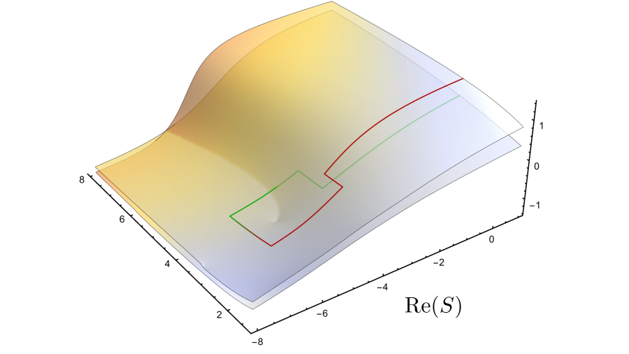
Figure 9: As we encircle the branch points around $S\simeq-5.5\pm 3.3i$ (see figure 8) families $2$ and $3$ get swapped. Here we plotted the integrability charge $q$ (or rather $f(q)=\arctan\left(\text{Im}(q)/20\right)$ which leads to a prettier plot) around that branch point to illustrate this. Two sheets of this function meet at that branch point. Of course, since the operators themselves are getting swapped, any quantity that probes them – such as the anomalous dimensions, the structure constants or any other correlator involving them – would produce a similar picture. We used a grid of $1.7\times 10^{6}$ points to generate this plot. Around $\text{Re}(S)=-8$ we encircle two other branch points which connect to a third sheet which is not represented here to ease visualization. Crossing these branch cuts with similar monodromies lead to the fourth even spin trajectory, see figure 8.

4.2 How it is derived: integrability

To generate energies at complex spin and construct the rich Riemann surfaces and associated monodromies, we diagonalize the Baxter operator, whose action on light-rays is discussed in appendix C. In practice, we solve the twist-three Baxter equation

$$Q(u+i)(u+i/2)^{3}+Q(u-i)(u-i/2)^{3}=Q(u)\times(\underbrace{2u^{3}-(S^{2}+2S+3/2)u+q}_{t(u)})\,,$$ (55)

with $S$ complex. One algorithm for solving this equation was suggested in [13]; it works perfectly for $S$ in the right half-plane but it does not work for $\text{Re}(S)<-1$. We suggest here an alternative algorithm very close in spirit to [18] which works for any $S$ and agrees with the one in [13] for $\text{Re}(S)>-1$. The algorithm is based on three simple steps:

• For any $q$, there exist two special solutions to the Baxter equation with pure power asymptotics. We define them through their behavior as we go up, $u\to+i\infty$,

  $$Q_{-2-S}(u) =u^{-2-S}+a_{1}u^{-3-S}+a_{2}u^{-4-S}+\dots\,,$$

  $$Q_{S}(u) =u^{S}+b_{1}u^{S-1}+b_{2}u^{S-2}+\dots\,.$$ (56)

  Importantly, note that the leading power is canonically normalized to $1$, and furthermore note that plugging such expansions into the Baxter equation allows us to fix completely all $a_{j}$ and $b_{j}$. For example,

  $$a_{1}=-\frac{q}{2S+3},\qquad a_{2}=\frac{q^{2}}{4(S+2)(2S+3)}+\frac{1}{48}(S+2)\left(S^{2}+4S+6\right)\,,\qquad\text{etc}.$$ (57)

  So as a first step in the algorithm we compute the functions $\hat{Q}_{-2-S}$ and $\hat{Q}_{S}$ given as a large $u$ expansion truncated after $N$ terms $\{a_{1},\dots,a_{N}\}$ and $\{b_{1},\dots,b_{N}\}$. For $N$ large, such functions $\hat{Q}_{-2-S}$ and $\hat{Q}_{S}$ are excellent approximations to ${Q}_{-2-S}$ and ${Q}_{S}$ as long as $u$ has a big imaginary part. How big should the imaginary part be and for a given large cut-off $N$ can be found experimentally checking for proper convergence.

• The functions $Q_{S}$ and $Q_{-2-S}$ are holomorphic in the upper half plane but they are singular in the lower half plane. Indeed, suppose we have a solution to the Baxter equation in the upper half place, valid for for some large imaginary part $u$. Using Baxter repeatedly we can lower the imaginary part in integer steps. Explicitly we have

  $$Q(u)=\frac{t(u+i)Q(u+i)-Q(u+2i)(u+3i/2)^{3}}{(u+i/2)^{3}}\,.$$ (58)

  so that the right hand side will develop a third order pole at $u=-i/2$ unless the numerator is carefully tuned. This pole at $u=-i/2$ then propagates to $-3i/2$ and then to $-5i/2$ etc. To construct fully holomorphic solutions to Baxter thus requires tuning and — in particular — it requires dropping pure power asymptotics. Instead we consider

  $$Q_{\text{holomorphic}}(u)\equiv(e^{2\pi u}+c_{0}+c_{1}e^{-2\pi u})\,Q_{-2-S}(u)+c_{2}Q_{S}(u),$$ (59)

  which of course solves Baxter as long and $Q_{-2-S}$ and $Q_{S}$ do. Then we tune the three constants $c_{0},c_{1},c_{2}$ to require that the third-, second- and first-order pole at $u=-i/2$ vanishes. Once the function is regular at this point, it will no longer generate poles at $-3i/2,-5i/2,\dots$ and will thus be holomorphic everywhere. At infinity it behaves as $e^{2\pi u}u^{-2-S}$ which we assume is the correct behavior for the $Q$-functions.

  In practice we use the approximate solutions $\hat{Q}_{-2-S}$ and $\hat{Q}_{S}$ to obtain in this way an approximate solution $\hat{Q}_{\text{holomorphic}}$.

• Note that up to now we have constructed (approximate) holomorphic solutions for any complex spin $S$ and complex charge $q$. Lastly, we quantize $q$ by imposing the zero momentum condition

  $$0=Q_{\text{holomorphic}}(i/2)-Q_{\text{holomorphic}}(-i/2)\,.$$ (60)

  Numerically solving this equation, e.g. with Newton’s method, will lead to many $q$’s for each complex spin $S$. The various solutions are the various Regge trajectories!

  In practice we change $S$ adiabatically. We find some $q$ corresponding to the $n$-th Regge trajectory for some complex spin $S$ and then we change $S$ slightly and use that previous value of $q$ as a starting point for a new scan of (60). In this way we can follow $Q$ (and thus the corresponding charges including the energy) as we follow arbitrarily complicated paths in the complex $S$ plane! Sometimes we find that under closed paths $Q$’s acquire monodromies and do not come back to themselves. This is fine; it simply means they live on a Riemann surface and that different Regge trajectories are actually different branches of the very same master function. As long as our complex spin $S$ paths do not get too close to the branch points of this Riemann surface, the numerics will be fast and stable.

• Finally, to extract energies, one can consider the expansion of the quantized $Q_{\text{holomorphic}}$ at $u\pm i/2$,

  $$\gamma(S)=2\left(Q^{\prime}(-i/2)-Q^{\prime}(i/2)\right)/Q(i/2).$$ (61)

Note that the Baxter equation (55), the holomorphicity condition, the zero momenta condition (60) and the asymptotics (59) are not new conditions but instead should follow from the action of the Baxter operator on the light-rays constructed in section 2. Indeed, we discuss how to derive all these properties in appendix C, with the exception of the asymptotics which we only managed to derive for $L=2$. In particular, we discuss how, in the light-ray language, one can simply derive Janik’s $Q$-function from the twist two light-ray wave function (39).

4.3 How it could in principle have been derived: dispersion relation

Could we have derived such nice Riemann surfaces with all their various sheets from a clever analytic continuation of the integer spin data, in the spirit of Newton’s method employed in [13] without any of the fancier methods just developed?

In principle Yes.

In this section we explain how. As a warm up suppose we want to take a trivial integral that we know how to compute very well for integer spin, namely,

$$I_{2}(S)\equiv\frac{1}{2}\int\limits_{-1}^{+1}dz\,(P_{S}(z))^{2}=\frac{1}{2S+1}.$$ (62)

Suppose we are given (62) for $S=0,1,2,3,\dots$. How can we analytically continue this integral away from the integers to reproduce the expected result $1/(2S+1)$ for any complex spin? What we should not do is use Mathematica blindly: NIntegrate[LegendreP[S,z]^2,{z,-1,1}]/2 does not give $1/(2S+1)$ unless $S$ is integer. Why do we like $1/(2S+1)$ as an continuation to complex spin compared to what Mathematica gives and which we plot in figure 10?

The key difference is that $1/(2S+1)$ does not blow up exponentially for large complex spin. By Carlson’s theorem, it is the unique analytic continuation of the integer sequence $\{1/1,1/3,1/5,1/7,1/9,\dots\}$ with this property. Mathematica’s continuation does blow up. This can be seen from the asymptotics of $\verb"LegendreP[S,z]"$, which read for $|z|\leq 1$

$${P_{S}(-z)}\sim\frac{1}{\sqrt{S}}\left(e^{iS\theta}+e^{-iS\theta}\right),\qquad z=\cos\theta,$$ (63)

which diverges with exponential type $\pi$ in the right-half plane (violating Carlsons assumptions). The oscillations in figure 10 are actually a sign of such $e^{2\pi iS}$ like terms which oscillate when $S$ is real but explode for complex $S$. Of course, it is easy to cook up combinations of such oscillations as in $\sin(\pi S)$ which vanish for all the integers which is why Mathematica’s continuation passes through all the correct black dots in the figure despite being wrong as long as we are after the non-exploding unique continuation.

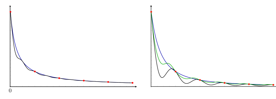
Figure 10: (a) Blue: $2/(2S+1)$. Black: $\int_{-1}^{1}P_{S}(x)^{2}dx$ which can be evaluated with Mathematica’s continuation of the Legendre polynomials. They agree at the integers. (b) Blue: non-exponential analytic continuation from the integers as described in this section. Black: continuation of the sum in equation (6) of [13]. Green: $\int_{-1}^{1}P_{S}(x)^{4}dx$ from Mathematica.

Let’s then set Mathematica aside and try to be cleverer in our analytic continuation. We want to start with integer $S$ and do some massaging to arrive at an expression where there are no $S$ oscillations as we continue to complex $S$. The trick is to do a few cleaver contour manipulations that will end up transforming an oscillating contour integral into an exponentially damped integral over a simple discontinuity. We were inspired from the same type of manipulations performed in Regge theory to make sense of partial waves at complex spin, see [4].

We start with

$$\frac{1}{2}\int\limits_{-1}^{1}dx\,P_{S}(x)^{2},$$ (64)

which for integer $S$ is obviously equal to

$$\oint\frac{dt}{2\pi i}\frac{1}{t^{S+1}}F(t)\qquad\text{where}\qquad F(t)=\sum_{S^{\prime}=0}^{\infty}\frac{t^{S^{\prime}}}{2}\int\limits_{-1}^{1}dx\,P_{S^{\prime}}(x)^{2}$$ (65)

Now note that to compute $F(t)$ all we need to do it add up integer spin $S^{\prime}$ for which we do know (62). We obtain that $F(t)$ is a nice holomorphic function in the plane minus a single cut for $t>1$,

$$F(t)=\sum_{S^{\prime}=0}^{\infty}\frac{t^{S^{\prime}}}{2S^{\prime}+1}=\frac{1}{2\sqrt{t}}\log\left(\frac{1+\sqrt{t}}{1-\sqrt{t}}\right).$$ (66)

Now we blow the contour integral in (65) so it becomes

$$\int_{1}^{\infty}\frac{dt}{t^{S+1}}\frac{\text{Disc}(F)(t)}{2\pi i}.$$ (67)

The discontinuity of (66) is trivial so we end up simply with

$$\frac{1}{2}\int_{1}^{\infty}\frac{dt}{t^{S+3/2}}=\frac{1}{2S+1},$$ (68)

as we wanted. The key was going from (65) to (67). In this second representation the integrand is manifestly damped. As such this representation should now be free from oscillations and thus ought to yield the unique continuation a la Carlson theorem. And it did indeed.

This was too trivial of an example. Lets try a much more interesting integral where the values at the first few integer values of $S$ are by no means enough to guess the general result,

$$I_{3}(S)\equiv\frac{1}{2}\int\limits_{-1}^{+1}dx(P_{S}(x))^{4}=\left\{1,\frac{1}{5},\frac{3}{35},\frac{241}{5005},\frac{529}{17017},\dots\right\}\quad\,\quad S=0,1,2,3,4,\dots\,.$$ (69)

This is not a random example. Structure constants of the lowest twist three trajectory are given by the this integral up to trivial combinatorial factors. In [13] we dealt with the analytic continuation of this integral by Newton Method; here we will instead use a numerical implementation of the method employed above. The match between the two methods is perfect as depicted in figure 10b.

1. First we construct

   $$\tilde{F}(t)\equiv\sum_{S^{\prime}=0}^{S_{\text{max}}}I_{3}(S^{\prime})t^{S^{\prime}},$$ (72)

   This function will have a cut at $t=1$ as in our analytic example (66). However, we can not simply go to $t\pm i0$ with $t>1$ to see this log since the Taylor expansion in $t$ will only converge in a radius $1$ circle around the origin.

2. To solve this limitation we introduce the uniformizing variable

   $$\rho(t)=\frac{\sqrt{1-t}-1}{\sqrt{1-t}+1},$$ (73)

   which maps the cut plane $\mathbb{C}-(1,\infty)$ to the unit disk and re-expand (72) to define

   $$\tilde{\tilde{F}}(\rho)=\sum_{S=0}^{S_{\text{max}}}c_{S}\rho^{S}.$$ (74)

   This function with two tildes is fixed to have the same expansion around $t=0$ (corresponding to the center of the unit disk) as (72) but it now converges everywhere in the $\rho$ unit disk! This allows us to access any $t$ in the cut plane!

3. Finally, we can now estimate the discontinuity of ${F}(t)\equiv\sum_{S^{\prime}=0}^{\infty}I_{3}(S^{\prime})t^{S^{\prime}}$ for $t>1$ as

   $${F}(t+i0)-{F}(t-i0)=\tilde{\tilde{F}}(\rho)-\tilde{\tilde{F}}(1/\rho),$$ (75)

   with $\rho$ in the upper arc of the unit disk.

4. Assuming we can blow the contour up in the general case, the desired integral can then be approximated by inserting (75) in (67) for $z>1$. We then recover the smooth dark blue curve in (b) of figure 10, reproducing the continuations of the structure constants obtained in [13] using Newton’s series.

One can also successfully reproduce the Newton series continuation of the higher twist three families through this procedure. This provides a new perspective on the decoupling zeroes of [13]. We define, in the even twist three case,

$$F(t)=\sum_{n=S^{*}_{k}/2}^{\infty}\left(f_{(S\equiv 2n),k}\equiv\frac{\Gamma(2n+1)^{2}}{\Gamma(4n+2)C_{2n,k}^{2}}\right)t^{n-S*_{k}/2},$$ (76)

where the index $k$ label the various classically degenerate twist three trajectories which starts at spin $S^{*}_{k}$. This definition of $f$ applied to twist $2$ or for the lowest familty of twist three would lead precisely to $f=I_{2}$ and $f=I_{3}$, the two examples considered above. Suppose that $f_{S}\sim e^{\alpha S}S^{\beta}$ at large $S$. Then the series converges for $te^{\alpha}<1$. Experimentally we observed $\alpha=0$.

We claim that $F(t)$ is polynomially bounded with a single cut at $|t|>1$. This in turns implies that $f_{S,k}$ are analytic in spin, which can be made manifest by writing the dispersive representation

$$f_{S,k}=\int_{1}^{\infty}dt\frac{\text{disc}F(t)}{t^{\tfrac{1}{2}(S-S^{*}_{k})+1}},$$ (77)

where we drop the contour at infinity (and obtain a convergent expression) for large enough $S$ due to polynomial boundedness of $F(t)$. This can be evaluated numerically following the four step method just outlined.

Combining the analyticity of $f_{S,k}$ with the analyticity of $C_{S,k}^{2}$ lead to a number of interesting observations:

• $C_{S,k}$ is analytic in the right half plane (RHP), which in turn implies that $f_{S,k}$ can never vanish in the RHP.

• $f_{S,k}$ is analytic for $S>S_{*}$ if and only if $C_{S,k}^{2}$ has definite sign for $S>S_{*}$.

• Indeed, in [13] we observed that $C_{S,k}^{2}$ is positive for $S>S_{k}^{*}$. In fact, the only zeroes in the RHP are the decoupling zeroes at the even integers smaller than $S_{k}^{*}$. This in turn is equivalent to

  $$\text{disc}F(t)=\sum_{n=1}^{S^{*}_{k}/2}\frac{a_{n}}{t^{n}}+o(t^{-S^{*}_{k}/2}).$$ (78)

  Can (a refined version of) this be proved in general CFT?

• From our new investigations we know that $C_{S,k}^{2}$ has branch points with ramification index $2$ at points $S_{b_{i}}$, $b_{i}$ standing for branch point $i$. The question arises: how this can be generated from (77)? These are obtained from specific logarithmic decay of $\text{disc}F(t)$. Specifically, the asymptotic terms

  $$\text{disc}F(t)\sim t^{(S_{b_{i}}-S^{*}_{k})/2}(\log t)^{-m/2}$$ (79)

  with $m\in\mathbb{Z}$ produces a branch point at $S=S_{b_{i}}$ with ramification index $2$ upon integration.

In sum: From purely integer spin data we can construct a function $F(t)$; with clever coordinates we can explore $F(t)$ beyond its naive convergence domain given by its Taylor series. Moreover, the asymptotic behavior of such a function at large $t$ contains formidable information! In principle information about its various cuts can even be extracted as in (79). This can thus in principle be used an alternative method to rederive the Riemann surfaces of the previous section as long as we have a monumental amount of integer data to play with as well as ingenious fit methods to extract such asymptotic behaviors from well constructed extrapolations. Does it work in practice? See footnote 22. See also footnote 25.

Hopefully we can learn better spectroscopy methods to make this approach more competitive.

5 CFT cousin trajectories

The black trajectories in figure 2 provide an analytic continuation in spin of the even-spin twist-three spectrum. They are realized by the light-ray operators constructed in section 2, and naturally appear in the Regge limit of four point correlators.

It is natural to ask whether these analytic continuations are unique. Namely, is there a different way of organizing the spectrum into analytic trajectories? This was one of the questions posed in the introduction. In section 2, we argued that the black trajectories correspond to light-ray operators of the form (10) with sufficiently smooth kernels at coincident points, or, equivalently, light-ray operators (10) that diagonalize $\mathbb{D}_{1}$. Nevertheless, this does not exclude the possibility of other analytic continuations existing, even if they are not realized by light-rays of the form (10).

The Newton series (30) provides a numerical strategy to explore this question. Under the assumption of analyticity in the right half $S$ plane and sufficiently tame asymptotic growth in this regime [31, 32], e.g. exponential type less than $\log(2)$, Newton series converges in the right half-plane. One can then reverse the logic: plugging a selection of even integer values in the right-half plane one can test for convergence of (30). This is how the black trajectories, and the decoupling zeroes of the structure constants of higher trajectories, were originally identified in [13].

In this section we

• Explore this strategy to argue that there exist alternative analytic continuations of the CFT spectrum.

• Identify how to define these trajectories from integrability, at the level of the quantum numbers.

• Speculate on their operator realization and list some open questions.

We will omit the operators on the $q=0$ lowest trajectory throughout figures in this section. We should think of them as living in a different symmetry sector as discussed in footnote 14.

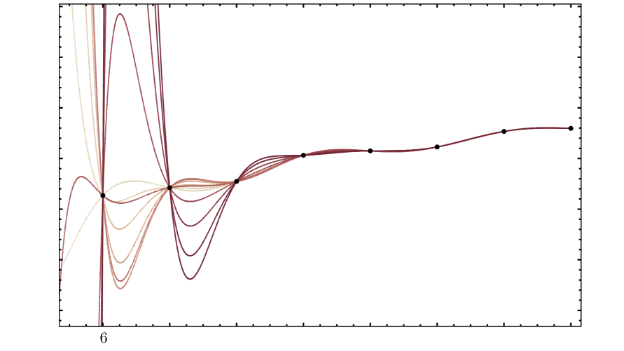
Figure 11: The partial sums (80) defining Newton’s series constructed with the integer spin red points in figure 2 - the highest anomalous dimension operators at every even spin. From light-colored to dark red $n_{\text{max}}$ ranges from ten to twenty. The partial sums diverge as more integer points to the right are included in the interpolation. This is expected since there should not be an analytic trajectory satisfying good Regge behavior and analytic in the right half-plane which interpolates the red operators. A similar result would be obtained by applying Newton’s series to, e.g., $f(S)=1/((S-10)^{2}+1)$ or $f(S)=e^{\log(3)S}$.

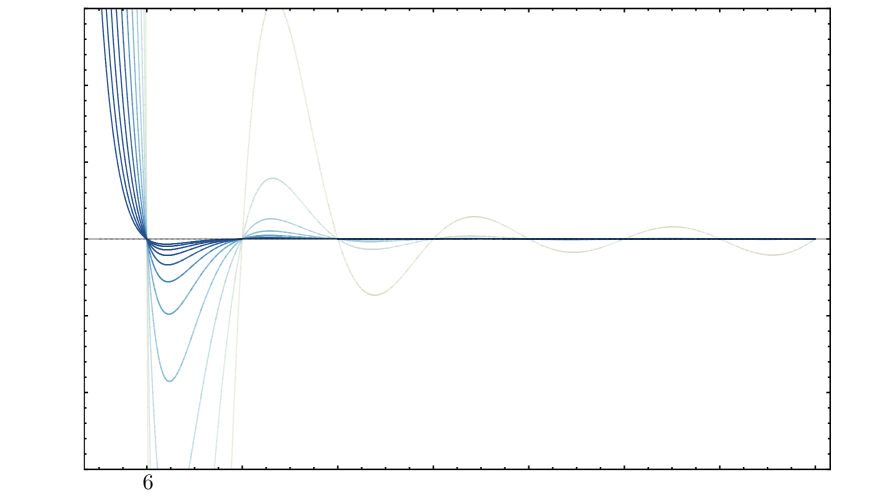
Figure 12: For the black trajectories of figure 2 the Newton partial sums converge everywhere in the right half-plane. From light-colored to navy $n_{\text{max}}$ ranges from ten to fourty in steps of four. We plot the error between the partial sums and the ‘exact’ result computed from the Baxter function.

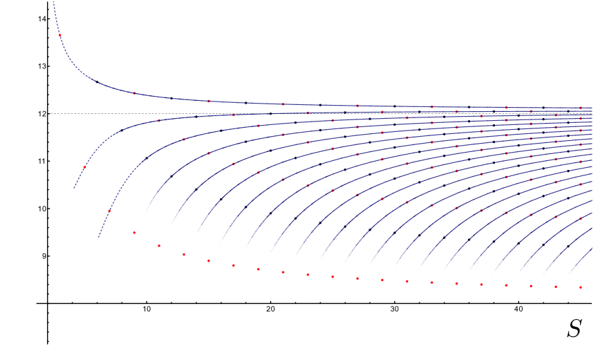
Figure 13: Twist three single-trace operators in $\mathcal{N}=4$ SYM can be organized into analytic trajectories in infinitely many ways. Here we organize the spectrum by assigning operators from top to bottom of the spectrum into families. They interpolate physical operators every three units of spin (and thus mix even and odd spin operators). The solid curves in the figure are produced using Newton’s interpolation using only the even spin (black points) operators — that they interpolate the odd spin (red points) is automatic. We fade these curves to the left as they start to lose precision. The dashed curves are produced using Baxter equation as explained in the main body of this section. They perfectly agree with Newton’s interpolation. For the first three trajectories we continue them to the left, where Newton’s partial sum is not perfectly accurate numerically. More generally, the Baxter equation can be used to construct these trajectories in the full complex spin plane as in section 4.

Figure 14: The even spin $n=4$ trajectories. They interpolate operators in spin steps of $12$. It is not clear if they are bounded from above or below.

Let us first illustrate that not anything goes. For example, consider the assignment of operators defined by the red curve in figure 2. In figure 11.(a) we plot the partial sums defined by Newton polynomials

$$\gamma_{n_{\text{max}}}(S)=\sum_{n=0}^{n_{\text{max}}}\binom{\tfrac{S-6}{2}}{n}\sum_{i=0}^{n}(-1)^{n-i}\binom{n}{i}\gamma^{\text{red}}_{6+2i},$$ (80)

where we use the first $n_{\text{max}}+1$ even operators along the red curve. Compare this with figure 12, where we display the analogous exercise for the second lowest black trajectory of figure 2. We interpret the result of this exercise as indication that the red list of operators do not form an analytic trajectory (holomorphic on a half plane, with good Regge behaviour at large $S$), while the black list does (as derived from Baxter or from the light-ray construction).

We do, however, identify an infinite number of ways of assigning operators into analytic trajectories! They are peculiar in that these trajectories interpolate the spectrum not in steps of two, but in steps of multiples of three!

Before describing these trajectories in full generality, let us discuss the first non-trivial example, considered in figure 13. These families interpolate operators in steps of three. The various trajectories are indexed by an integer $\ell\geq 0$ and the operators in each trajectory are indexed by $k\geq 1$. Trajectory $\ell$ interpolates the $(1+\lfloor\ell/3\rfloor)$-th operator with highest dimension at spin $3k+2\ell$. Note that the number of operators at each spin increases in steps of six, hence the origin of the $\lfloor\ell/3\rfloor$ factor, see appendix A. Note that operators are organized from top to bottom, and hence it is not clear if the trajectories are bounded from below. Moreover, these trajectories mix even and odd spin data under analytic continuation!

These trajectories were in practice identified through Newton’s series. Plugging the selected local operators in Newton’s formula results in beautiful numerical convergence which we interpret as indication that the CFT data indeed extends into an analytic function satisfying the basic properties required for Newton’s series convergence. Indeed, note that one could reconstruct this analytic trajectory using only the even spin data along the trajectories using

$$\gamma^{\text{steps of 3}}_{\ell}(S)=\sum_{n=0}^{\infty}\binom{\tfrac{S-6-2\ell}{6}}{n}\sum_{i=0}^{n}(-1)^{n-i}\binom{n}{i}\gamma^{(1+\lfloor\ell/3\rfloor)\text{-th operator}}_{6+2\ell+6i}.$$ (81)

One can then recover the odd spin spectrum from (81). One obtains a perfect match with the direct computation of the odd spin spectrum. Indeed, the solid curves in figure 13 were generated using only even spin data through (81). That the red points are interpolated comes automatically.

Although we identified these trajectories with Newton’s method, we understand how to construct them directly at complex spin using the Baxter equation. They are described by solutions of the Baxter equation (55) for entire functions with asymptotics $e^{2\pi u}u^{-2-S}$ as in section 4, but we must drop the zero-momenta condition $Q(i/2)=Q(-i/2)$ in favor of the deformed condition $Q(i/2)=e^{\frac{2(S-2l)i\pi}{3}}Q(-i/2)$! We thank Simon Caron-Huot for this suggestion. Imposing this condition fixes $q$ precisely as predicted by the Newton series (which can be applied directly for the $q$ charges). The anomalous dimension extracted from the Baxter function perfectly matches the solid curves in figure 13. Indeed, the dashed curves in figure 13 are generated with Baxter equation and extend the curves beyond the regime in which we have strong numerical control with Newton’s series. The Baxter equation thus opens the way to explore the full complex plane structure of these new “steps of three” trajectories. We anticipate that these various trajectories are connected by branch cuts and form a unique Riemann surface as in section 4, only that now even and odd spin operators are on the same surface.

Infinitely many other assignments are possible. These assignments can be characterized by their “spin step” $3n$ with integer $n\geq 3$. They interpolate operators of spin $S=3nk+S_{0}$ for integer $k\geq 0$. If a given trajectory interpolates the $m$-th highest dimension operator at spin $S$, then it interpolates the $(m+1)$-th highest dimension operator at spin $S+3n$. We illustrate the assignment $n=4$ in figure 14. Baxter functions associated with these continuations can be constructed through the quantization condition $Q(i/2)=e^{\frac{2(S-S_{0})i\pi}{3n}}Q(-i/2)$.

6 Discussion

In this work, we explicitly constructed light-ray operators in ${\cal N}=4$ SYM whose anomalous dimensions and matrix elements provide an analytic continuation in spin of multi-twist local operators. The wavefunctions of these light-ray operators satisfy integral and differential equations coming from integrability. These equations can be solved systematically in a kind of discrete Fourier space, allowing us to plot solutions and numerically compute operator norms and matrix elements. The appropriate solutions satisfy falloff conditions in Fourier space, which give restrictions on the types of singularities the wavefunctions possess at coincident points. These falloff conditions lead to quantization of the integrable charge $q$, and also to discrete Regge trajectories. With explicit light-ray operators in hand, we can also confirm the picture of [13, 14]: there are an infinite number of Regge trajectories, but only a finite number of them have nonzero matrix elements at each integer spin.

An important ingredient in computing matrix elements of our light-ray operators is the light-ray “norm” of [15, 14]. Our implementation of this norm involves starting with a time-ordered correlator of $2L$ constituent partons, and then integrating them against light-ray wavefunctions. This clearly gives a pairing between wavefunctions, but it is less clearly a pairing between two separate light-ray operators. A nonperturbative approach to this norm is used in [14], where they start with a time-ordered four-point function of local operators and integrate it against a pair of bi-local kernels. These two constructions do not correspond to each other in an obvious way, yet they both seem to give consistent results. Can we formulate a more natural definition of a time-ordered correlator of light-ray operators?

The anomalous dimensions of our complex-spin light-ray operators can alternatively be computed from the Baxter equation, by constructing solutions with the correct holomorphicity conditions and large-$u$ asymptotics. Results from the Baxter equation exactly match those coming from our explicit numerical light-ray wavefunctions. Using the Baxter equation, we can also continue further into the complex plane, revealing a rich Riemann surface that unifies naïvely different Regge trajectories. It is interesting to ask how this Riemann surface interacts with other trajectories such as BFKL trajectories and shadow trajectories that can intersect the Riemann surface at special values of $S$, presumably through a generalization of [19, 33] to non-parity symmetric trajectories. It would also be interesting to trace how light-ray wavefunctions change in the vicinity of branch points connecting different Regge trajectories. Furthermore, it would be nice to develop methods for computing light-ray matrix elements using separation of variables/integrability without explicitly constructing the wavefunctions, possibly opening the way to computing these observables away from weak coupling.

An alternative approach to computing data of twist-three light-ray operators in ${\cal N}=4$ SYM was recently presented in [29]. A central idea of [29] is to, instead of working with light-ray operator wavefunctions directly, study correlators of local operators in the presence of a light-ray operator. Such correlators are related by a series of integral transforms to the wavefunctions we compute in this work. The approach of [29] gives an alternative way to efficiently access anomalous dimensions in the right-half $S$ plane.

Although we have developed a relatively complete picture for the simplest analytic continuation in spin of multi-twist trajectories, we also found a surprise: there exist infinitely many other ways of assembling local operators into analytic “cousin” trajectories. These cousin trajectories require changing the quantization condition of the Baxter function, which suggests that they involve modifying cyclicity of the trace. Perhaps we can interpret them as light-ray versions of the “color twist operators” of [34]. Are these cousin trajectories an accident of planar integrability in ${\cal N}=4$ SYM, a feature of single-trace trajectories in large-$N$ gauge theory, or are they a general property of the multi-twist spectrum in CFT? These questions can be tested in particular examples with Newton’s series. One particularly interesting feature of cousin trajectories is that they connect even- and odd-spin operators together into a unified object. Is this also a quirk of ${\cal N}=4$ SYM, or does it reflect something more general?

Cousin trajectories have anomalous dimensions asymptoting to $\gamma_{S}=3\Gamma_{\text{Cusp}}\log S$ at large spin. This is to be contrasted with non-cousin trajectories, whose anomalous dimensions asymptote to $\gamma_{S}=2\Gamma_{\text{Cusp}}\log S$. At integer spin, the $3\Gamma_{\text{Cusp}}\log S$ behavior can be understood from the local operator wave function, which is dominated by spin equally distributed between the various partons. The energy is dominated by the color flux connecting neighboring partons [35]. Holographically, they correspond to a string made of three folds which approach the boundary of AdS. The folds are connected by a Y-junction which does not approach the boundary. [36, 37]. By contrast, the $2\Gamma_{\text{Cusp}}\log S$ behavior corresponds to local operators whose wave function is dominated by two partons having small relative spin or, holographically, the junction approaching the boundary. It would be interesting to understand these asymptotics from a complex spin perspective. This story is remarkably similar to that of sister trajectories in string theory, whose large spin semiclassics corresponds to spinning strings with extra folds - and thus increased tension [38, 39].

Other natural questions about light-ray operators are also interesting to ask about cousin trajectories. The standard analytic trajectories appear naturally in conformal Regge theory [16, 4, 12, 40], where they describe the behavior of four-point correlators in the Regge limit. What kinematic limit is described by light-ray operators on cousin trajectories? What is the complete story at higher-twist? What do the light-ray wavefunctions of cousin trajectories look like? Using Newton’s series one can construct the analytic continuation of the integrable charge $q$ associated to the trajectories of figure 13. We learn that, for these trajectories, the quantized values of $q$, at fixed $S$, correspond precisely to the values for which the function $\log(\alpha_{2}/\alpha_{1})$ depicted in figure 3 diverges! In other words, for the values of $q$ corresponding to these trajectories there exist maximally asymmetric solutions of the recursion relation, with Fourier modes asymptotics $a_{n}\simeq n^{-1}$ for $n\rightarrow\infty$ while $a_{n}\simeq n^{S}$ for $n\rightarrow-\infty$. It would be interesting to explore this further.

We opened this work reminiscing on the stiff analytic structure imposed on the spectrum of CFTs by large boost physics. We conclude by noting that, at least in $\mathcal{N}=4$ SYM, likely in holographic CFTs, and ambitiously in general, the story goes much further. Not only operators must organize in analytic families, they must do so in infinitely many ways. How far can we push this incredibly rigid constrain when bootstrapping this and other theories? And what other secrets about the structure of CFTs does Lorentizan physics still hold?

Appendix A Counting higher-twist trajectories

In this appendix, we provide the counting of primary operators at a given spin $S$. The first part of the analysis is performed for general $L$. We then focus on $L=3$.

For each $L$, to compute the number of single-trace primary states at spin $S$ it is enough to compute the dimension of the space of single-traces of spin $S$, $n_{L}(S)$. The number of primaries at spin $S$ is then given by $n_{L}(S)-n_{L}(S-1)$. We therefore focus on the computation of $n_{L}(S)$.

The problem of determining $n_{L}(S)$ is equivalent to the problem of determining the number of permutations of a set of $S+L$ elements, $S$ of which and $L$ of which are indistinguishable, modulo cyclic permutations. In simpler terms, we would like to make a “necklace” using “beads” of two “colors”, $L$ of which being blue and $S$ of which being red. We aim to count how many necklaces can be made. Before solving this problem, let us consider a simpler but instructive problem.

Problem 1 Let us relax the condition that we have $L$ and $S$ beads of each color respectively. Let us simply build necklaces of length $K$ using $m$ colors without tracking how many of each beads of each colors were used.

Consider the set $X$ of all sequences of $K$ beads. We would like to identify those that are equivalent under the action of the cyclic group $G=\mathbb{Z}/K\mathbb{Z}$ and count the number of distinct equivalent classes. In other words, we want to count the number of orbits of the action of $G$ on $X$, $|X/G|$. The result is provided by Burnside Lemma.

Burnside Lemma Suppose one is given a set $X$ and an action of a finite group $G$ onto $X$. Denote by $|X^{g}|$ the number of elements in $X$ that are left invariant by an element $g\in G$. The number of orbits of the action of $G$ onto $X$, $|X/G|$ is given by the average number of fixed points of the action. That is:

$$|X/G|=\frac{1}{|G|}\sum_{g\in G}|X^{g}|.$$ (82)

Proof: let $f(g,x)=1$ if $g.x=x$ and zero otherwise. Then

$$\frac{1}{|G|}\sum_{g\in G}|X^{g}| =\frac{1}{|G|}\sum_{g\in G}\sum_{x\in X}f(g,x)$$ (83)

$$=\frac{1}{|G|}\sum_{x\in X}\sum_{g\in G}f(g,x)$$ (84)

$$=\frac{1}{|G|}\sum_{x\in X}|\text{Stab}(x)|,$$ (85)

where $|\text{Stab}(x)|$ is the number of elements $g$ that stabilize $x$. But $|\text{Stab}(x)|=|G|/|O_{x}|$ where $|O_{x}|$ is the number of elements in the orbit of $x$ (this is the orbit-stabilizer theorem). We then get

$$\frac{1}{|G|}\sum_{g\in G}|X^{g}| =\frac{1}{|G|}\sum_{x\in X}\frac{|G|}{|O_{x}|}$$ (86)

$$=\sum_{x\in X}\frac{1}{|O_{x}|}=|X/G|,$$ (87)

since each orbit $O$ contributes $\frac{1}{|O|}$ $|O|$ times.

Solution of problem 1

Given a cyclic permutation $g\in G$, how many necklaces are fixed by the action of $g$? A necklace is fixed by the action of $g$ if and only if each cycle of $g$ has a definite color. Suppose that $g$ has $c(g)$ cycles. Then

$$|X^{g}|=m^{c(g)},$$ (88)

where $m$ is the number of colours available to build the necklace.

An element $g\in\mathbb{Z}/K\mathbb{Z}$ has $d$ cycles of length $K/d$, where $d=gcd(K,g)$, the greatest common divisor of $K$ and $g$. The number of possible necklaces of length $K$ is then

$$|X/G| =\frac{1}{K}\sum_{g=1}^{K}m^{gcd(g,K)}$$ (89)

$$=\frac{1}{K}\sum_{d|K}\phi\left(\tfrac{K}{d}\right)m^{d},$$ (90)

where the sum in the second equality is over the divisors of $K$. $\phi(x)$ is the Euler (totient) $\phi$ function, which counts the numbers of positive integers $y$ smaller than $x$ that are relative prime to $x$ (i.e. $gcd(y,x)=1$). The last equality is true because if $gcd(g,K)=d$ then $d|K$, $d|g$ and $gcd(K/d,m/d)=1$.

Back to counting of primaries

Equation (90) provides the solution to problem 1. We can think of (90) as a partition function. Each quantum number $d$ has degeneracy $\phi(K/d)$, and each state contributes with the number of possible colorings $m^{d}$. Our original problem requires us to restrict the allowed colorings by requiring that out of the $K=L+S$ beads, $L$ of them are red and $S$ of them are blue. We introduce chemical potential $r$ and $b$ associated to red and blue beads respectively. The partition (generating) function then becomes

$$Z_{L,S}(r,b)=\frac{1}{K}\sum_{d|K}\phi\left(\tfrac{K}{d}\right)\left(r^{\tfrac{K}{d}}+b^{\tfrac{K}{d}}\right)^{d}.$$ (91)

We interpret each term in the sum as assigning color $r$ or $b$ to each of the cycles $d$ of the original element $g$. Each cycle has $\frac{K}{d}$ elements which must have the same colour. The number of single traces states $n_{L}(S)$ is then simply the coefficient of $r^{L}b^{S}$ in the polynomial (91).

Figure 15: Number of twist three primaries as a function of spin. Blue: odd trajectories. Red: even trajectories. They are given by expression (95).

Twist three primaries

Let us set $L=3$ and ask for the coefficient of $b^{3}$ in (91). We can set $r=1$ without loss of information. There are only two terms in the sum that can contribute, $d=K$ or $d=K/3$. The latter only contributes if $S$ is a multiple of three. Using that $\phi(1)=1$ and $\phi(3)=2$, we obtain that

$$n_{3}(S)=\left\{\begin{array}[]{ll}(S+1)(S+2)/6&\mbox{if }S/3\notin\mathbb{Z},\\ (S+3)S/6+1&\mbox{if }S/3\in\mathbb{Z}.\end{array}\right.$$ (92)

Note that both answers are integers, as one can check with basic modular arithmetic. The number of primaries $p_{3}(S)=n_{3}(S)-n_{3}(S-1)$ at a given spin $S$ is then

$$p_{3}(S)=\left\{\begin{array}[]{ll}(S+1)/3&\mbox{if }S\equiv 1\mod 3,\\ (S-1)/3&\mbox{if }S\equiv 2\mod 3,\\ 1+S/3&\mbox{if }S\equiv 0\mod 3.\end{array}\right.$$ (93)

To recognize the familiar functions quoted in the introduction, let us consider values of $S\mod 6$:

$$p_{3}(S)=\left\{\begin{array}[]{ll}(S-1)/3=2\lfloor S/6\rfloor=2\lfloor(S+4)/6\rfloor&\mbox{if }S\equiv 1\mod 6,\\ (S-1)/3=2\lfloor S/6\rfloor+1&\mbox{if }S\equiv 4\mod 6,\\ (S+1)/3=2\lfloor S/6\rfloor+1&\mbox{if }S\equiv 2\mod 6,\\ (S+1)/3=2\lfloor S/6\rfloor+2=2\lfloor(S+4)/6\rfloor&\mbox{if }S\equiv 5\mod 6,\\ S/3+1=2\lfloor S/6\rfloor+2=2\lfloor(S+4)/6\rfloor&\mbox{if }S\equiv 3\mod 6,\\ S/3+1=2\lfloor S/6\rfloor+1&\mbox{if }S\equiv 6\mod 6.\\ \end{array}\right.$$ (94)

We therefore conclude that

$$p_{3}(S)=\left\{\begin{array}[]{ll}2\lfloor(S+4)/6\rfloor&\mbox{if }S\in 2\mathbb{Z}+1,\\ 2\lfloor S/6\rfloor+1&\mbox{if }S\in 2\mathbb{Z},\end{array}\right.$$ (95)

as promised. See figure 15.

Appendix B Details of perturbative computations

B.1 Twist 2

In this subsection we expand on the computation of the twist two light-ray correlators $\langle\mathcal{O}_{1}\mathbb{O}\mathcal{O}_{2}\rangle$ and $\langle\mathcal{T}\{\mathbb{O}\bar{\mathbb{O}}\}\rangle_{\text{g.f.}}$.

To compute $\langle\mathcal{O}_{1}\mathbb{O}\mathcal{O}_{2}\rangle$ let us set $y=0$ and $z=n^{+}$ in (39). We take $x_{1}^{-}>0$ and $x_{2}^{+}<0$. There are two possible Wick contractions. They are related by $(\alpha_{1}\leftrightarrow\alpha_{2})$, which is a symmetry of the wave function, and therefore amounts to a factor of two. In the end, the computation results in

$$\langle\mathcal{O}_{1}(x_{1})\mathbb{O}\mathcal{O}_{2}(x_{2})\rangle=\frac{i\sqrt{2}\sqrt{\Gamma(2S+1)}}{2\pi\Gamma(S+1)x^{2}_{12}}\int d\alpha_{1}d\alpha_{2}\frac{\left(\alpha_{1}-\alpha_{2}+i\epsilon\right)^{-1-S}}{\left(\alpha_{1}x_{1}^{-}+x_{1}^{2}+i\epsilon\right)\left(\alpha_{2}x_{2}^{-}+x_{2}^{2}+i\epsilon\right)},$$ (96)

where the second factor in the wave function vanishes by contour deformation. Both integrals are performed by residues, deforming the contour away from the branch cut in the imaginary direction. The final result is

$$\langle\mathcal{O}_{1}(x_{1})\mathbb{O}\mathcal{O}_{2}(x_{2})\rangle=\left(2\pi i\frac{\Gamma(2S+1)}{\Gamma(S+1)^{2}}\right)C_{\mathcal{O}_{S}O_{1}O_{2}}(S)\frac{\left(\tfrac{x_{1}^{2}}{x_{1}^{-}}-\tfrac{x_{2}^{2}}{x_{2}^{-}}\right)}{x_{1}^{-}x_{2}^{-}x_{12}^{2}}^{-1-S},$$ (97)

which is quoted in (42).

Next, we want to compute (44) which we reproduce here:

$$\langle\mathcal{T}\{\mathbb{O}\bar{\mathbb{O}}\}\rangle_{\text{g.f.}}=\frac{\Gamma(2S+1)}{4\pi^{2}\Gamma(S+1)^{2}}\int\prod_{i=1}^{2}d\alpha_{i}d\beta_{i}\frac{\lambda\delta(\alpha_{1}+\alpha_{2}-\lambda)\psi(\alpha_{1},\alpha_{2})\psi(\beta_{1},\beta_{2})}{(\alpha_{1}\beta_{1}+d^{2}+i\epsilon)(\alpha_{2}\beta_{2}+d^{2}+i\epsilon)}.$$ (98)

Before proceeding with the direct computation, let us emphasize a couple of nice properties of (98):

• The integrals over $\beta_{i}$ vanish unless $\alpha_{1}$ and $\alpha_{2}$ have opposite sign. To see this, suppose they are positive, and deform $\beta_{i}$ into the lower half plane, away from the propagator poles. In each term of the wave function, see (39), only either $\beta_{1}$ or $\beta_{2}$ will have singularities in the lower-half plane. One of the integrals thus vanishes, as seen by the contour deformation.

• On the other hand, for even values of $S$, the wave functions have no support when $\alpha_{i}$ have opposite sign, see discussion under (1).

We thus expect that, for even spin, when the light-ray reduces to $L[\mathcal{O}_{S}]$, the continuous spin norm defined by ${\langle\mathcal{T}\{\mathbb{O}\bar{\mathbb{O}}\}\rangle_{\text{g.f.}}}/{\langle 0|\mathbb{O}\bar{\mathbb{O}}|0\rangle}$ vanishes. We thus see that the conversion between the continuous spin norm and the continuation in $S$ of the canonical norm of the local operators $\mathcal{O}_{S}$ — which equals one — must involve dividing by zeroes at every even integer. We will see this explicitly.

To compute (98), let us instead perform the integrals over $\beta_{i}$ by picking the poles of the propagators. Change variables as $u=\alpha_{1}+\alpha_{2}$, $v=\alpha_{1}-\alpha_{2}$. The integral in $u$ is fixed by the gauge-fixing. Since $\alpha_{i}$ must have opposite sign, it is enough to integrate over $|v|>\lambda$. In fact, from permutation symmetry of $\psi(\alpha_{1},\alpha_{2})$ we can restrict to $v>\lambda$ up to a factor of two. We will use the fact that $\psi(\alpha_{1},\alpha_{2})=\left(1+e^{i\pi(-1-S)}\right)|v|^{-1-S}$. The integral reduces to

$$\frac{4\Gamma(2S+1)}{\Gamma(S+1)^{2}}\left(1+e^{i\pi(-1-S)}\right)\lambda\int_{v>\lambda}dv\frac{v^{-1-S}}{\lambda^{2}-v^{2}}\left(\frac{2d^{2}}{v+\lambda}+\frac{2d^{2}}{v-\lambda}\right)^{-1-S}=-\frac{\left(1+e^{i\pi(-1-S)}\right)}{(2S+1)d^{2+S}}.$$ (99)

The factor in the numerator realizes the manifest zeroes described above. The denominator, in a similar manner to what happened in the three-point matrix element case, can be understood from the (double) light-transform of the canonical two-point structure. Indeed, see [12],

$$\langle 0|L[\mathcal{O}_{S}]L[\bar{\mathcal{O}}_{S}]|0\rangle=\frac{-2\pi i}{\tau+2S-1}\langle 0|\mathbb{O}\bar{\mathbb{O}}|0\rangle={\frac{-2\pi i}{(2S+1)d^{2+S}}},$$ (100)

where $\langle 0|\mathbb{O}\bar{\mathbb{O}}|0\rangle$ is the canonical two-point structure for operators of dimension $1-S$ and spin $1-\Delta$. In the last equality we specified our coordinate frame and twist two. We thus conclude that

$$\frac{\langle\mathcal{T}\{\mathbb{O}\bar{\mathbb{O}}\}\rangle}{\langle 0|\mathbb{O}\bar{\mathbb{O}}|0\rangle}=-\left(1+e^{i\pi(-1-S)}\right)/(2S+1).$$ (101)

B.2 Twist 3

In this appendix we examine the computation of $\langle\mathcal{O}_{1}\mathbb{O}_{n,S}\mathcal{O}_{2}\rangle$ and ${\langle\mathcal{T}\{\mathbb{O}_{n,S}\bar{\mathbb{O}}_{n,S}\}\rangle}$.

We parametrize twist three light-rays $\mathbb{O}_{n,S}$ inserted at $x=-\infty n^{+}$, $z=n^{+}$ as

$$\mathbb{O}_{n,S}=\int d\alpha_{\text{cm}}drd\theta\left(\psi\left(\alpha_{cm},r,\theta\right)\equiv\frac{1}{\Gamma(S_{n}^{*}-S)}\frac{g_{n,S}(\theta)}{r^{1+S}}\right)\text{Tr}\left(\mathcal{Z}(\alpha_{1})\mathcal{Z}(\alpha_{2})\mathcal{Z}(\alpha_{3})\right),$$ (102)

with $\alpha_{i}$ being parametrized by $(\alpha_{cm},r,\theta)$ according to (15-17) as

$$\alpha_{i} =\alpha_{cm}+\tfrac{1}{3}r\alpha_{i}^{\theta},$$ (103)

$$\alpha_{i}^{\theta} =\cos(\theta-2\pi(i-1)/3)-\cos(\theta-2\pi(i-2)/3).$$ (104)

We introduce the $\Gamma$ function factor for later convenience, where $S_{n}^{*}=6(n-1)$ is the first integer spin in which the $n$-th even trajectory has physical operators, see figure 2.

The computation of the matrix elements $\langle\mathcal{O}_{1}\mathbb{O}_{n,S}\mathcal{O}_{2}\rangle$ is straightforward. We take $\mathcal{O}_{1}={\rm Tr}\left(\mathcal{X}\bar{\mathcal{Z}}\right)$ and $O_{2}={\rm Tr}\left(\bar{\mathcal{X}}\bar{\mathcal{Z}}^{2}\right)$ and consider $x_{1}^{-}>0$, $x_{2}^{-}<0$. All Wick contractions are equivalent due to cyclic symmetry of the wave function, and amount to a factor of six. We thus want to compute

$$\langle\mathcal{O}_{1}\mathbb{O}_{n,S}\mathcal{O}_{2}\rangle=6\int d\alpha_{\text{cm}}drd\theta\frac{\psi\left(\alpha_{cm},r,\theta\right)(x_{2}^{-}\alpha_{3}+x_{2}^{2}+i\epsilon)^{-1}}{(x_{1}^{-}\alpha_{1}+x_{1}^{2}+i\epsilon)(x_{2}^{-}\alpha_{2}+x_{2}^{2}+i\epsilon)}.$$ (105)

The integral over $\alpha_{cm}$ can be performed by deforming the contour into the lower half-plane, picking up the pole at $\alpha_{cm}/3=-x_{1}^{2}/x_{1}^{-}-r\alpha_{1}^{\theta}-i\epsilon$. The integral over $r$ can also be performed by residues by realizing that distributionally

$$\int_{\mathbb{R}^{+}}drr^{-1-S}f(r)=\int_{\mathbb{R}}dr\frac{e^{-i\pi(1+S)}(r-i\epsilon)^{-1-S}-e^{i\pi(1+S)}(r+i\epsilon)^{-1-S}}{2i\sin(\pi S)}f(r).$$ (106)

One can then perform the integral over $r$ in each term by deforming away from the branch-points in the imaginary direction, thus picking the propagator poles. The final result for $\langle\mathcal{O}_{1}\mathbb{O}_{n,S}\mathcal{O}_{2}\rangle$ is

$$\frac{12i\pi^{2}3^{-S}}{x_{1}^{-}(x_{2}^{-})^{2}\sin(\pi S)\Gamma(S^{*}_{n}-S)}\left(\frac{x_{1}^{2}}{x_{1}^{-}}-\frac{x_{2}^{2}}{x_{2}^{-}}\right)^{-2-S}\int d\theta g(\theta)\frac{\left({\alpha_{3}^{\theta}-\alpha_{1}^{\theta}}-i\epsilon\right)^{1+S}-\left({\alpha_{2}^{\theta}-\alpha_{1}^{\theta}}-i\epsilon\right)^{1+S}}{(\alpha_{3}^{\theta}-\alpha_{2}^{\theta})},$$ (107)

which must be evaluated numerically for each trajectory as we will discuss later. From (107) we read that the kernel of (51) is

$$F_{\text{three points}}(\theta)=12i\pi^{2}3^{-S}\times\frac{\left({\alpha_{3}^{\theta}-\alpha_{1}^{\theta}}-i\epsilon\right)^{1+S}-\left({\alpha_{2}^{\theta}-\alpha_{1}^{\theta}}-i\epsilon\right)^{1+S}}{(\alpha_{3}^{\theta}-\alpha_{2}^{\theta})}.$$ (108)

Next, let us consider the computation of the norm $\langle\mathcal{T}\{\mathbb{O}\bar{\mathbb{O}}\}\rangle_{\text{g.f.}}$. We will consider the same crosswise kinematical configuration as in the twist-2 case, see figure 6. We use the gauge fixing $\delta(r_{\alpha}-1)$. In a similar manner to the previous case, the correlator vanishes if all $\alpha_{i}$ have the same sign. We can use cyclicity and reflection symmetry of the $\psi(\alpha_{i})$ wave function, equations (13) and (14), to restrict to the case $\alpha_{1}>0$, $\alpha_{2}<0$, $\alpha_{3}<0$. All planar Wick contractions can be related by cyclicity of the wave function $\psi(\beta_{i})$. In sum, we would like to compute

$$\langle\mathcal{T}\{\mathbb{O}\bar{\mathbb{O}}\}\rangle_{\text{g.f.}}=18\int_{\begin{subarray}{c}\alpha_{1}>0\\ \alpha_{2}<0\\ \alpha_{3}<0\end{subarray}}\frac{dr_{\alpha}d\alpha_{cm}d\theta_{\alpha}dr_{\beta}d\beta_{cm}d\theta_{\beta}\delta(r_{\alpha}-1)\psi_{\mathbb{O}}\left(\alpha_{cm},r_{\alpha},\theta_{\alpha}\right)\psi_{\bar{\mathbb{O}}}\left(\beta_{cm},r_{\beta},\theta_{\beta}\right)}{(\beta_{1}\alpha_{1}+d^{2}+i\epsilon)(\beta_{2}\alpha_{2}+d^{2}+i\epsilon)(\beta_{3}\alpha_{3}+d^{2}+i\epsilon)}.$$

The integrals over $\beta_{cm}$ and $r_{\beta}$ can be performed by picking the propagator poles, as in the three-point matrix element computation. The integral over $r_{\alpha}$ is localized. We are left with a triple integral

$$\langle\mathcal{T}\{\mathbb{O}\bar{\mathbb{O}}\}\rangle_{\text{g.f.}}=\frac{(d^{2})^{-1-S}}{\sin(\pi S)\Gamma(S_{n}^{*}-S)^{2}}\int_{D}d\alpha_{cm}d\theta_{\alpha}d\theta_{\beta}g_{\mathbb{O}}(\theta_{\alpha})g_{\bar{\mathbb{O}}}(\theta_{\beta})\times$$ (109)

$$\begin{array}[t]{@{}c@{}}\underbrace{\left(\frac{\left(\left((\alpha_{cm}+\alpha_{1}^{\theta})(-\alpha_{cm}-\alpha_{2}^{\theta})\right)^{1+S}F_{1}(\theta_{\alpha},\theta_{\beta})-\left((\alpha_{cm}+\alpha_{1}^{\theta})(-\alpha_{cm}-\alpha_{3}^{\theta})\right)^{1+S}F_{2}(\theta_{\alpha},\theta_{\beta})\right)}{(-36\pi^{2}i(3)^{-2S}e^{i\pi(S+1)})^{-1}\left(F_{3}(\theta_{\alpha},\theta_{\beta})+\alpha_{cm}F_{4}(\theta_{\alpha},\theta_{\beta})\right)}\right)}\\ F_{\text{two point}}(\theta_{\alpha},\theta_{\beta},\alpha_{cm})\end{array},$$ (112)

from which we read the kernel $F_{\text{two point}}$ of (52) which is defined in terms of

$$F_{1}(\theta_{\alpha},\theta_{\beta}) =\left(\frac{\alpha_{1}^{\theta}-\alpha_{2}^{\theta}}{\beta_{1}^{\theta}-\beta_{2}^{\theta}}+i\epsilon\right)^{-1-S},\qquad F_{2}(\theta_{\alpha},\theta_{\beta})=\left(\frac{\alpha_{1}^{\theta}-\alpha_{3}^{\theta}}{\beta_{1}^{\theta}-\beta_{3}^{\theta}}+i\epsilon\right)^{-1-S},$$

$$F_{3}(\theta_{\alpha},\theta_{\beta}) =\alpha_{1}^{\theta}\beta_{1}^{\theta}(\alpha_{2}^{\theta}-\alpha_{3}^{\theta})+\alpha_{2}^{\theta}\beta_{2}^{\theta}(\alpha_{3}^{\theta}-\alpha_{1}^{\theta})+\alpha_{3}^{\theta}\beta_{3}^{\theta}(\alpha_{1}^{\theta}-\alpha_{2}^{\theta}),$$

$$F_{4}(\theta_{\alpha},\theta_{\beta}) =\beta_{1}^{\theta}(\alpha_{2}^{\theta}-\alpha_{3}^{\theta})+\beta_{2}^{\theta}(\alpha_{3}^{\theta}-\alpha_{1}^{\theta})+\beta_{3}^{\theta}(\alpha_{1}^{\theta}-\alpha_{2}^{\theta})$$

and we re-scaled $\alpha_{cm}\rightarrow\alpha_{cm}/3$. The domain of integration $D$ is given by $\alpha_{cm}>-\alpha_{1}^{\theta}$, $\alpha_{cm}<-\alpha_{2}^{\theta}$, $\alpha_{cm}<-\alpha_{3}^{\theta}$. The integral over $\alpha_{cm}$ can be evaluated analytically. We do not use this fact.

Finally, in order to be able to write (51) and (52) we define our choices of two- and three- point structures. In our conformal frames, we choose

$$\langle 0|\mathbb{O}\bar{\mathbb{O}}|0\rangle=(d^{2})^{-1-S}\qquad\text{and}\qquad\langle 0|\mathcal{O}_{1}\mathbb{O}\mathcal{O}_{2}|0\rangle=\frac{1}{x_{1}^{-}(x_{2}^{-})^{2}}\left(\frac{x_{1}^{2}}{x_{1}^{-}}-\frac{x_{2}^{2}}{x_{2}^{-}}\right)^{-2-S}.$$ (113)

Appendix C Q-functions from light-rays

In section 2, we emphasized that light-ray operators in $\mathcal{N}=4$ SYMs should diagonalize the transfer-matrix operator, whose action on light-rays of arbitrary twist is defined through equation (21). The transfer matrix operator was very useful due to its simple differential action. Its polynomial eigenvalues are sufficient to completely characterize the state.

The light-rays should also diagonalize the Baxter $\mathbb{Q}$ operator. It act as an integral operator [41]

$$\mathbb{Q}(u)\circ\mathbb{O}=\frac{\cosh(\pi u)^{L}}{\pi^{L}}\int_{0}^{1}\prod_{j=1}^{L}dz_{j}(1-z_{j})^{iu-1/2}(z_{j})^{-iu-1/2}\times$$

$$\int_{-\infty}^{\infty}\prod_{i=1}^{L}d\alpha_{i}\psi(\alpha_{1},\dots,\alpha_{L})\text{Tr}\left[\mathcal{Z}(z_{1}\alpha_{1}+(1-z_{1})\alpha_{L})\dots\mathcal{Z}(z_{L}\alpha_{L}+(1-z_{L})\alpha_{L-1}))\right],$$ (114)

and is especially useful due to serving as a generating function of (infinitely many) integrable charge operators

$$\mathbb{C}_{k}^{\pm}=2i^{k+1}\left(\mathbb{Q}^{(k)}(i/2)\mp\mathbb{Q}^{(k)}(-i/2)\right).$$ (115)

In particular, the dilatation operator, whose action was defined in (31), is given by $\mathbb{D}=\mathbb{C}^{+}_{1}$. Note that the Baxter operator is an entire function of $u$. The poles of the integral in (114) at $u=k\pm i/2$ cancel with the zeroes of the trigonometric prefactor. The prefactor is normalized so that

$$\mathbb{C}^{+}_{0}=1,$$ (116)

which follows from cyclicity of the trace.

The eigenvalues

$$\mathbb{Q}(u)\circ\mathbb{O}=Q(u)\mathbb{O}$$ (117)

can be obtained without reference to $\psi$. This is the strategy adopted in section (4) in order to uncover the operator mixing in the spin left half-plane. For that, one uses the operatorial Baxter equation

$$\mathbb{Q}(u+i)(u+i/2)^{L}+\mathbb{Q}(u-i)(u-i/2)^{L}=\mathbb{Q}(u)\tau(u).$$ (118)

Acting on a light-ray operator produces the Baxter equation (55) but, crucially, note that the various quantization conditions for complex spin, first proposed by Janik in the twist two context [30] and generalized to higher twist in [13], are here fixed given general properties determing the light-ray wave functions. In particular, as argued above, the zero momentum condition

$$Q(i/2)=Q(-i/2)$$

holds at complex spin due to cyclicity of the trace defining light-ray operators, the analyticity of $Q(u)$ follows from the analyticity of $\mathbb{Q}$, and, we expect, the leading asymptotics of $Q(u)$ are fixed by the Lorentz spin of the light-ray $J_{L}$

$$\lim_{u\rightarrow\infty}Q(u)\propto e^{2\pi u}u^{J_{L}}+\dots\,,$$ (119)

where $J_{L}=1-L-S$, see section 2.2, thus providing a physical explanation for the decaying solution of Janik. These three properties, combined with the Baxter equation (55), uniquely fix all Baxter eigenfunctions corresponding to the twist three trajectories at any value of the spin. In section 4 we discuss how to do so numerically and present results for twist three.

We have not been successful in deriving the result (119) for general $L$. However, it is interesting to see that, for $L=2$, (119) — and, therefore, Janik’s $Q$-function — can be derived from the light-ray wave function $\psi_{2}$. To do so, we start from (114). Changing variables as $(z_{i}\alpha_{i}+(1-z_{i})\alpha_{i-1})\rightarrow\alpha_{i}$ we obtain

$$\mathbb{Q}(u)\circ\mathbb{O}=\frac{\cosh(\pi u)^{2}}{\pi^{2}}\int_{0}^{1}\prod_{j=1}^{2}dz_{j}(1-z_{j})^{iu-1/2}(z_{j})^{-iu-1/2}\times$$

$$\int_{-\infty}^{\infty}\prod_{i=1}^{2}d\alpha_{i}|1-z_{1}-z_{2}|^{-1}\psi_{2}\left(\frac{\alpha_{i}}{-1+z_{1}+z_{2}}\right)\text{Tr}\left[\mathcal{Z}(\alpha_{1})\mathcal{Z}(\alpha_{2}))\right].$$ (120)

Using that $\psi_{2}(\lambda\alpha_{i})=|\lambda|^{J_{2}\equiv-S-1}\psi_{2}(\alpha_{i})$ we get

$$\mathbb{Q}(u)\circ\mathbb{O}=\Bigg{(}Q_{2}(u)=\frac{\cosh(\pi u)^{2}}{\pi^{2}}\int_{0}^{1}dz_{1}g(z_{1})\times$$ (121)

$$\left(\int_{0}^{1-z_{1}}dz_{2}(1-z_{1}-z_{2})^{S}g(z_{2})+\int_{1-z_{1}}^{1}dz_{2}(-1+z_{1}+z_{2})^{S}g(z_{2})\right)\Bigg{)}\times\mathbb{O}$$

with $g(x)=(1-x)^{iu-1/2}(x)^{-iu-1/2}$. At large $u$, the integrals can be performed by saddle point. The saddles are located at $z_{1}-z_{2}=0$, $z_{1}+z_{2}=1$. The large $u$ behaviour of $Q_{2}(u)\sim u^{-1-S}$ is then manifest. Of course, the integrals above are of the Euler type and can be performed exactly, matching Janik’s Q-function at finite $u$.

References

- [1] A.L. Fitzpatrick, J. Kaplan, D. Poland and D. Simmons-Duffin, The Analytic Bootstrap and AdS Superhorizon Locality, JHEP 12 (2013) 004 [1212.3616].
- [2] Z. Komargodski and A. Zhiboedov, Convexity and Liberation at Large Spin, JHEP 11 (2013) 140 [1212.4103].
- [3] A.L. Fitzpatrick, J. Kaplan, M.T. Walters and J. Wang, Eikonalization of Conformal Blocks, JHEP 09 (2015) 019 [1504.01737].
- [4] S. Caron-Huot, Analyticity in Spin in Conformal Theories, JHEP 09 (2017) 078 [1703.00278].
- [5] S. Caron-Huot, M. Kologlu, P. Kravchuk, D. Meltzer and D. Simmons-Duffin, Detectors in weakly-coupled field theories, 2209.00008.
- [6] I. Balitsky, V. Kazakov and E. Sobko, Two-point correlator of twist-2 light-ray operators in N=4 SYM in BFKL approximation, Nucl. Phys. B 993 (2023) 116267 [1310.3752].
- [7] R.C. Brower, J. Polchinski, M.J. Strassler and C.-I. Tan, The Pomeron and gauge/string duality, JHEP 12 (2007) 005 [hep-th/0603115].
- [8] T. Jaroszewicz, Gluonic Regge Singularities and Anomalous Dimensions in QCD, Phys. Lett. B 116 (1982) 291.
- [9] L.N. Lipatov, Small x physics in perturbative QCD, Phys. Rept. 286 (1997) 131 [hep-ph/9610276].
- [10] A.V. Kotikov and L.N. Lipatov, NLO corrections to the BFKL equation in QCD and in supersymmetric gauge theories, Nucl. Phys. B 582 (2000) 19 [hep-ph/0004008].
- [11] A.V. Kotikov and L.N. Lipatov, DGLAP and BFKL equations in the supersymmetric gauge theory, Nucl. Phys. B 661 (2003) 19 [hep-ph/0208220].
- [12] P. Kravchuk and D. Simmons-Duffin, Light-ray operators in conformal field theory, JHEP 11 (2018) 102 [1805.00098].
- [13] A. Homrich, D. Simmons-Duffin and P. Vieira, Complex Spin: The Missing Zeroes and Newton’s Dark Magic, 2211.13754.
- [14] J. Henriksson, P. Kravchuk and B. Oertel, Missing local operators, zeros, and twist-4 trajectories, 2312.09283.
- [15] S. Caron-Huot, When does the gluon reggeize?, JHEP 05 (2015) 093 [1309.6521].
- [16] M.S. Costa, V. Goncalves and J. Penedones, Conformal Regge theory, JHEP 12 (2012) 091 [1209.4355].
- [17] M. Alfimov, N. Gromov and V. Kazakov, QCD Pomeron from AdS/CFT Quantum Spectral Curve, JHEP 07 (2015) 164 [1408.2530].
- [18] N. Gromov, F. Levkovich-Maslyuk and G. Sizov, Quantum Spectral Curve and the Numerical Solution of the Spectral Problem in AdS5/CFT4, JHEP 06 (2016) 036 [1504.06640].
- [19] R. Klabbers, M. Preti and I.M. Szécsényi, Regge spectroscopy of higher twist states in supersymmetric Yang-Mills theory, 2307.15107.
- [20] P.A.M. Dirac, Wave equations in conformal space, Annals Math. 37 (1936) 429.
- [21] G. Mack and A. Salam, Finite component field representations of the conformal group, Annals Phys. 53 (1969) 174.
- [22] S. Ferrara, A.F. Grillo, G. Parisi and R. Gatto, Covariant expansion of the conformal four-point function, Nucl. Phys. B 49 (1972) 77.
- [23] S. Ferrara, A.F. Grillo and R. Gatto, Tensor representations of conformal algebra and conformally covariant operator product expansion, Annals Phys. 76 (1973) 161.
- [24] S. Weinberg, Six-dimensional Methods for Four-dimensional Conformal Field Theories, Phys. Rev. D 82 (2010) 045031 [1006.3480].
- [25] M.S. Costa, J. Penedones, D. Poland and S. Rychkov, Spinning Conformal Correlators, JHEP 11 (2011) 071 [1107.3554].
- [26] L.D. Faddeev, How algebraic Bethe ansatz works for integrable model, in Les Houches School of Physics: Astrophysical Sources of Gravitational Radiation, pp. pp. 149–219, 5, 1996 [hep-th/9605187].
- [27] N. Beisert, The Dilatation operator of N=4 super Yang-Mills theory and integrability, Phys. Rept. 405 (2004) 1 [hep-th/0407277].
- [28] “Bootstrap 2023 talks.” Conference Website.
- [29] S. Caron-Huot, “Bootstrap meets integrability lectures.” Youtube Link.
- [30] R.A. Janik, Twist-two operators and the BFKL regime - nonstandard solutions of the Baxter equation, JHEP 11 (2013) 153 [1309.2844].
- [31] R.C. Buck, Interpolation series, Transactions of the American Mathematical Society 64 (1948) 283.
- [32] N.E. Norlund, “Leçons sur les séries d’interpolation..” Gauthier-Villars (Collection de monographies sur la théorie des fonctions), 1926.
- [33] S. Ekhammar, N. Gromov and M. Preti, Long Range Asymptotic Baxter-Bethe Ansatz for N=4 BFKL, 2406.18639.
- [34] A. Cavaglia, D. Grabner, N. Gromov and A. Sever, Colour-twist operators. Part I. Spectrum and wave functions, JHEP 06 (2020) 092 [2001.07259].
- [35] L.F. Alday and J.M. Maldacena, Comments on operators with large spin, JHEP 11 (2007) 019 [0708.0672].
- [36] A.V. Belitsky, A.S. Gorsky and G.P. Korchemsky, Gauge / string duality for QCD conformal operators, Nucl. Phys. B 667 (2003) 3 [hep-th/0304028].
- [37] M. Kruczenski, Spiky strings and single trace operators in gauge theories, JHEP 08 (2005) 014 [hep-th/0410226].
- [38] D.J. Gross and P.F. Mende, String Theory Beyond the Planck Scale, Nucl. Phys. B 303 (1988) 407.
- [39] B. Basso, S. Caron-Huot and A. Sever, Adjoint BFKL at finite coupling: a short-cut from the collinear limit, JHEP 01 (2015) 027 [1407.3766].
- [40] S. Caron-Huot and J. Sandor, Conformal Regge Theory at Finite Boost, JHEP 05 (2021) 059 [2008.11759].
- [41] S.E. Derkachov, Baxter’s q-operator for the homogeneous xxx spin chain, Journal of Physics A: Mathematical and General 32 (1999) 5299.