Optimization by Parallel Quasi-Quantum Annealing with Gradient-Based Sampling

Abstract

Learning-based methods have gained attention as general-purpose solvers due to their ability to automatically learn problem-specific heuristics, reducing the need for manually crafted heuristics. However, these methods often face scalability challenges. To address these issues, the improved Sampling algorithm for Combinatorial Optimization (iSCO), using discrete Langevin dynamics, has been proposed, demonstrating better performance than several learning-based solvers. This study proposes a different approach that integrates gradient-based update through continuous relaxation, combined with Quasi-Quantum Annealing (QQA). QQA smoothly transitions the objective function, starting from a simple convex function, minimized at half-integral values, to the original objective function, where the relaxed variables are minimized only in the discrete space. Furthermore, we incorporate parallel run communication leveraging GPUs to enhance exploration capabilities and accelerate convergence. Numerical experiments demonstrate that our method is a competitive general-purpose solver, achieving performance comparable to iSCO and learning-based solvers across various benchmark problems. Notably, our method exhibits superior speed-quality trade-offs for large-scale instances compared to iSCO, learning-based solvers, commercial solvers, and specialized algorithms.

1 Introduction

Combinatorial optimization (CO) problems aim to find the optimal solution within a discrete space, a fundamental challenge in many real-world applications (Papadimitriou and Steiglitz, 1998; Crama, 1997). Most CO problems are NP-hard, making it challenging to solve large-scale problems within feasible computational time. As a result, developing algorithms that efficiently find high-quality approximate solutions has been a critical focus. Traditionally, heuristic methods have been widely used to find approximate solutions, but they require significant insights into the specific problems. Accordingly, increasing efforts have been directed toward developing general-purpose solvers that can be applied to a broad range of problems to reduce the need for problem-specific insights.

Among the general-purpose solvers, sampling-based approaches have been proposed, which treat CO problems as sampling problems. Simulated annealing (SA) (Kirkpatrick et al., 1983), a widely well-known technique, uses local thermal fluctuations and updates (Metropolis et al., 1953; Hastings, 1970). Additionally, techniques such as tempered transitions (Neal, 1996) and exchange Monte Carlo algorithms (Hukushima and Nemoto, 1996) have shown strong performance in practical CO problems (Johnson et al., 1989, 1991; Earl and Deem, 2005). However, these methods often depend on local updates, where only one dimension is updated at a time, and the update process across dimensions typically cannot be parallelized. As a result, these methods become computationally prohibitive when addressing large-scale CO problems.

Learning-based methods have recently gained recognition as general-purpose solvers for their ability to learn problem-specific heuristics automatically. This reduces the need for manually designed heuristics and leverages modern accelerators like GPUs and TPUs. Some learning-based methods rely on supervised data, which is often difficult to obtain (Li et al., 2018; Gasse et al., 2019; Gupta et al., 2020). Reinforcement learning (Khalil et al., 2017; Kool et al., 2018; Chen and Tian, 2019) and unsupervised learning approaches (Karalias and Loukas, 2020; Wang et al., 2022; Wang and Li, 2023) have expanded their applicability. However, these approaches encounter challenges when applied to out-of-distribution instances, limiting their flexibility in addressing a wide range of problem distributions. In response, unsupervised learning-based solvers that do not depend on training data have emerged, leveraging the ability of machine learning models to learn valuable representations (Schuetz et al., 2022a, b; Ichikawa, 2023). These methods address CO problems by optimizing the learning parameters of deep learning models, but model selection is critical in determining solution quality Schuetz et al. (2023). Furthermore, additional computational costs arise because the number of parameters typically exceed the number of discrete variables in the original CO problem. Moreover, the performance of these methods compared to sampling-based solvers remains unclear.

On the other hand, the improved Sampling algorithm for CO (iSCO) (Sun et al., 2023a) was proposed, motivated by advances in Markov Chain Monte Carlo methods for discrete space. This method integrates discrete Langevin dynamics (Sun et al., 2023b) with traditional annealing techniques, demonstrating results on par with, or better than, learning-based solvers by using gradient information from the objective function. This method efficiently utilizes GPUs via frameworks such as PyTorch and JAX, similar to learning-based methods. In this study, we propose a different method that combines gradient-based updates through continuous relaxation and Quasi Quantum Annealing (QQA) inspired by quantum annealing (Kadowaki and Nishimori, 1998). QQA gradually transitions the objective function, starting with a simple convex function minimized at half-integral values, similar to the state where the transverse field dominates in quantum annealing. This process leads to the original objective function, where the relaxed variables are minimized only within the discrete space, analogous to the classical state without the transverse field in quantum annealing. Unlike iSCO, our method introduces an extended Boltzmann distribution with a communication term between parallel runs, facilitating broader exploration with minimal overhead by effectively utilizing GPUs. This also accelerates convergence.

Numerical experiments on the same benchmark used as iSCO (Sun et al., 2023a), along with several other benchmarks, demonstrate that our method is a competitive general-purpose solver, achieving performance comparable to iSCO and learning-based solvers across all benchmarks. For larger problems, our method offers better speed-quality trade-offs than iSCO, learning-based solvers, commercial solvers, and specialized algorithms.

2 Background

Combinatorial Optimization.

The goal of this study is to solve CO problems formulated as

$$\min_{{\bm{x}}\in{\mathcal{X}}(C)}f({\bm{x}};C),~{}~{}{\mathcal{X}}(C)=\left\{{\bm{x}}\in\{0,1\}^{N}~{}\left|~{}~{}\begin{matrix}g_{i}({\bm{x}};C)\leq 0,&\forall i\in[I],\\ h_{j}({\bm{x}};C)=0&\forall j\in[J]\end{matrix}\right.\right\},$$ (1)

where $C\in{\mathcal{C}}$ denotes instance-specific parameters, such as a graph $G=(V,E)$, and ${\mathcal{C}}$ represents a set of all possible instances. The vector ${\bm{x}}=(x_{i})_{1\leq i\leq N}\in\{0,1\}^{N}$ represents the discrete decision variables, and ${\mathcal{X}}(C)$ denotes the feasible solution space. $f:{\mathcal{X}}\times{\mathcal{C}}\to{\mathbb{R}}$ is the cost function, while $g_{i}:{\mathcal{X}}\times{\mathcal{C}}\to{\mathbb{R}}$ and $h_{j}:{\mathcal{X}}\times{\mathcal{C}}\to{\mathbb{R}}$ represent inequality and equality constraints, respectively. We also use the shorthand notation $[N]=\{1,2,\ldots,N\}$, with $N\in{\mathbb{N}}$.

To transform the constrained CO problem into a sampling problem, we reformulate it as an unconstrained CO problem using the penalty method:

$$\min_{{\bm{x}}\in\{0,1\}^{N}}l({\bm{x}};C,{\bm{\lambda}}),~{}~{}l({\bm{x}};C,{\bm{\lambda}})\mathrel{\leavevmode\hbox{\set@color\hskip 3.8889pt\leavevmode\hbox{\set@color$=$}\raisebox{4.66875pt}{\leavevmode\hbox{\set@color$\scriptstyle\Delta$}}\hskip 3.8889pt}}f({\bm{x}};C)+\sum_{i=1}^{I+J}\lambda_{i}v_{i}({\bm{x}};C),$$ (2)

where $v_{i}:\{0,1\}^{N}\times{\mathcal{C}}\to{\mathbb{R}},\forall i\in[I+J]$ represents penalty terms, which increase as the constraints are violated. For example, these penalty terms can be defined as

$$\forall i\in[I],~{}v_{i}({\bm{x}};C)=\max(0,g_{i}({\bm{x}};C)),~{}~{}\forall j\in[J],~{}v_{j}({\bm{x}};C)=(h_{j}({\bm{x}};C))^{2}.$$ (3)

${\bm{\lambda}}=(\lambda_{i})_{1\leq i\leq I+J}\in{\mathbb{R}}^{I+J}$ denotes the penalty parameters that control the balance between constraint satisfaction and cost function minimization. As ${\bm{\lambda}}$ increases, these penalty terms grow, penalizing constraint violations more heavily.

Energy Based Model (EBM).

For the penalized objective function $l({\bm{x}};C,{\bm{\lambda}})$, we define the following Boltzmann distribution:

$$P({\bm{x}};T)=\frac{1}{{\mathcal{Z}}(T)}e^{-\frac{1}{T}l({\bm{x}};C,{\bm{\lambda}})},~{}~{}{\mathcal{Z}}(T)=\sum_{x\in{\mathcal{X}}}e^{-\frac{1}{T}l({\bm{x}};C,{\bm{\lambda}})},$$ (4)

where $T\in{\mathbb{R}}_{\geq 0}$ is a parameter called temperature, which controls the smoothness of the distribution. The summation $\sum_{{\bm{x}}}$ represents the sum over all possible values of ${\bm{x}}$. This distribution has the following property:

Proposition 2.1.

As the temperature $T$ approaches infinity, the Boltzmann distribution $P({\bm{x}};T)$ converges to a uniform distribution over $\{0,1\}^{N}$. When the temperature $T=0$, the Boltzmann distribution becomes a uniform distribution over the optimal solutions of Eq. (2).

Thus, the original CO problem can be transformed into a sampling problem from the probability distribution in Eq. 4 with $T=0$.

Metropolis–Hastings Algorithm.

The Metropolis–Hastings Algorithm (Metropolis et al., 1953; Hastings, 1970) is a general method for sampling from high-dimensional distributions. This algorithm uses a conditional distribution $Q$, called a proposal distribution, which satisfy the ergodicity condition. A Markov chain $({\bm{x}}^{(t)})_{t=0}^{T}$ is constructed to have $P({\bm{x}};T)$ as its stationary distribution by following steps; starting from ${\bm{x}}^{(0)}\sim P^{(0)}$, where $P^{(0)}$ is the initial distribution, at each step $t$, propose ${\bm{x}}^{\prime}\sim Q({\bm{x}}^{\prime}|{\bm{x}}^{(t)})$, and with probability

$$A({\bm{x}}^{\prime}|{\bm{x}}^{(t)})=\min\left(1,\frac{P({\bm{x}}^{\prime};T)Q({\bm{x}}^{(t)}|{\bm{x}}^{\prime})}{P({\bm{x}}^{(t)};T)Q({\bm{x}}^{\prime}|{\bm{x}}^{(t)})}\right)$$ (5)

accept ${\bm{x}}^{\prime}$ as the next state ${\bm{x}}^{(t+1)}={\bm{x}}^{\prime}$, or with probability $1-A({\bm{x}}^{\prime}|{\bm{x}}^{(t)})$, reject ${\bm{x}}^{\prime}$ and retain the previous state ${\bm{x}}^{(t+1)}={\bm{x}}^{(t)}$. The proposal distribution is typically a local proposal, such as a flipping a single bit. Gibbs sampling (Geman and Geman, 1984) is a local update method where the proposal distribution is the conditional distribution, $Q({\bm{x}}^{(t)}|{\bm{x}}^{\prime})=P(x^{(t)}_{i}|{\bm{x}}_{-i};T)$, with ${\bm{x}}_{-i}={\bm{x}}\setminus\{x_{i}\}$. In this case, the acceptance rate $A({\bm{x}}^{\prime}|{\bm{x}}^{(t)})$ is always $1$. The effectiveness of the algorithm is highly influenced by the choice of the proposal distribution $Q({\bm{x}}^{(t)}|{\bm{x}}^{\prime})$.

Simulated Annealing.

Simulated annealing (SA) was introduced by Kirkpatrick et al. (1983); Černỳ (1985). While the original optimization problem can be solved by sampling from the distribution $\lim_{T\to 0}P({\bm{x}};T)$, directly sampling from the distribution is difficult due to its highly nonsmooth nature at low temperatures. To overcome, SA performs Metropolis–Hastings updates while gradually lowering the temperature $T$ to zero through a temperature path, ${\mathcal{T}}=(T_{0},T_{1},\ldots,T_{M})$ where the path $T_{0}>T_{1}>\cdots>T_{M}\to 0$. This approach enables the system to reach a state with lower energy over time.

3 Method

We begin by explaining the continuous relaxation approach in Section 3.1. Section 3.2 introduces an extended Boltzmann distribution and QQA. Section 3.3 proposes the communication between parallel runs, and Section 3.4 summarizes optimization-specific techniques. This overall approach is termed Parallel Quasi-Quantum Annealing (PQQA).

3.1 Continuous Relaxation Strategy

The continuous relaxation strategy reformulates a CO problem into a continuous one by converting discrete variables into continuous ones as follows:

$$\min_{{\bm{p}}\in[0,1]^{N}}\hat{l}({\bm{p}};C,{\bm{\lambda}}),~{}~{}\hat{l}({\bm{p}};C,{\bm{\lambda}})\mathrel{\leavevmode\hbox{\set@color\hskip 3.8889pt\leavevmode\hbox{\set@color$=$}\raisebox{4.66875pt}{\leavevmode\hbox{\set@color$\scriptstyle\Delta$}}\hskip 3.8889pt}}\hat{f}({\bm{p}};C)+\sum_{i=1}^{m+p}\lambda_{i}\hat{v}_{i}({\bm{p}};C),$$

where ${\bm{p}}=(p_{i})_{1\leq i\leq N}\in[0,1]^{N}$ denotes the relaxed continuous variables, where each binary variable $x_{i}\in\{0,1\}$ is relaxed to a continuous value $p_{i}\in[0,1]$. $\hat{f}:[0,1]^{N}\times{\mathcal{C}}\to{\mathbb{R}}$ represents the relaxation of $f$, satisfying $\hat{f}({\bm{x}};C)=f({\bm{x}};C)$ for ${\bm{x}}\in\{0,1\}^{N}$. Similarly, for all $i\in[I+J]$, $\hat{v}_{i}$ denotes the relaxation of $v_{i}$, with $\hat{v}_{i}({\bm{x}};C)=v_{i}({\bm{x}};C)$ for ${\bm{x}}\in\{0,1\}^{N}$.

However, the landscape of relaxed objective function $\hat{l}({\bm{p}};C,{\bm{\lambda}})$ remains complex even after continuous relaxation, posing challenges for optimization. Moreover, continuous relaxation encounters rounding issues, where artificial post-rounding is needed to map the continuous solutions back to the original discrete space, undermining the robustness.

3.2 Quasi-Quantum Annealing

We represent the relaxed variable ${\bm{p}}\in[0,1]^{N}$ as a real-valued parameter ${\bm{w}}\in{\mathbb{R}}^{N}$ and a nonlinear mapping to evaluate gradients and introduce following entropy term to control the balance between continuity and discreteness of relaxed variables:

$$\hat{r}(\sigma({\bm{w}});C,{\bm{\lambda}},\gamma)=\hat{l}(\sigma({\bm{w}});C,{\bm{\lambda}})+\gamma s(\sigma({\bm{w}})),$$ (6)

where $\sigma:{\mathbb{R}}^{N}\to[0,1]^{N}$ denotes element-wise mapping, such as the sigmoid function and $\gamma\in{\mathbb{R}}$ denotes a penalty parameter. The relaxed variables are defined as $\sigma({\bm{w}})=(\sigma(w_{i}))_{1\leq i\leq N}\in[0,1]^{N}$. The entropy term $s(\sigma({\bm{w}}))$ is a convex function, which attains its minimum value of $0$ when $\sigma({\bm{w}})\in\{0,1\}^{N}$ and its maximum when $\sigma({\bm{w}})=\nicefrac{{{\bm{1}}_{N}}}{{2}}$. In particular, this study employs the following entropy:

$$s(\sigma({\bm{w}}))=\sum_{i=1}^{N}\left\{1-(2\sigma(w_{i})-1)^{\alpha}\right\},~{}~{}~{}\alpha\in\{2n\mid n\in{\mathbb{N}}\},$$ (7)

which was introduced by Ichikawa (2023) and is referred to as $\alpha$-entropy.

Furthermore, we extend the entropy term to general discrete optimization problems. Details of this generalization are provided in Appendix B. The effectiveness of this generalization is demonstrated through numerical experiments on two benchmarks: the balanced graph partitioning in Section 5.4 and the graph coloring problem in Section 5.5.

Subsequently, we extend the Boltzmann Distribution in Eq. (4) to the continuous space $[0,1]^{N}$ using Eq. (6) as follows:

$$\hat{P}(\sigma({\bm{w}});\gamma,T)=\frac{1}{{\mathcal{Z}}(\gamma,T)}e^{-\frac{1}{T}\hat{r}(\sigma({\bm{w}});C,{\bm{\lambda}},\gamma)},~{}~{}{\mathcal{Z}}(\gamma,T)=\int\prod_{i=1}^{N}dw_{i}e^{-\frac{1}{T}\hat{r}(\sigma({\bm{w}});C,{\bm{\lambda}},\gamma)}.$$ (8)

When $\gamma$ is negative, i.e., $\gamma<0$, the relaxed variables tend to favor the half-integral value $\sigma({\bm{w}})=\nicefrac{{{\bm{1}}_{N}}}{{2}}$, smoothing the non-convexity of the objective function $\hat{l}({\bm{p}};C,{\bm{\lambda}})$ due to the convexity of the penalty term $\Phi({\bm{p}})$. This state can be interpreted as a quasi-quantum state, where the values are uncertain between $0$ and $1$. Conversely, when $\gamma$ is positive, i.e., $\gamma>0$, the relaxed variables favor discrete values. This state can be interpreted as a classical state, where the values are deterministically determined as either $0$ or $1$. Formally, the following theorem holds.

Theorem 3.1.

Under the assumption that the objective function $\hat{l}({\bm{p}};C)$ is bounded within the domain $[0,1]^{N}$, the Boltzmann distribution $\lim_{\gamma\to+\infty}\lim_{T\to 0}\hat{P}(\sigma({\bm{w}});\gamma,T)$ converges to a uniform distribution over the optimal solutions of Eq. (2), i.e., ${\bm{x}}^{\ast}\in\mathrm{argmin}_{{\bm{x}}}l({\bm{x}};C,{\bm{\lambda}})$. Additionally, $\lim_{\gamma\to-\infty}\lim_{T\to 0}\hat{P}(\sigma({\bm{w}});\gamma,T)$ converges to a single-peaked distribution $\prod_{i=1}^{N}\delta(\sigma(w_{i})-\nicefrac{{1}}{{2}})$.

The detailed proof can be found in Appendix A.1.

The following gradient-based update can be used for any $\gamma$, provided that $r({\bm{w}})$ is differentiable:

$${\bm{w}}^{t+1}={\bm{w}}^{t}-\eta\nabla_{{\bm{w}}}r(\sigma({\bm{w}}^{t});C,{\bm{\lambda}})+\sqrt{2\eta T}{\bm{\xi}},$$ (9)

where $\eta$ is the time step, and ${\bm{\xi}}\sim\mathcal{N}({\bm{0}}_{N},I_{N})$ is Gaussian noise, with $I_{N}\in\mathbb{R}^{N\times N}$ denoting an identity matrix and ${\bm{0}}_{N}$ representing the zero vector $(0,\ldots,0)^{\top}\in\mathbb{R}^{N}$. This update rule generates a Markov chain whose stationary distribution is given by Eq. (8), provided that $\eta$ is sufficiently small. Unlike the local updates in conventional SA for discrete problems, this method simultaneously updates multiple variables in a single step via the gradient, allowing for high scalability.

Following Ichikawa (2023), annealing is conducted on $\gamma$ from a negative to a positive value while updating the parameter ${\bm{w}}$. Initially, a negative $\gamma$ is set to enable extensive exploration by smoothing the non-convexity of $\hat{l}(\sigma({\bm{w}});C,{\bm{\lambda}})$, where the quasi-quantum state $\sigma({\bm{w}})=\nicefrac{{{\bm{1}}_{N}}}{{2}}$ dominates. Subsequently, the penalty parameter $\gamma$ is gradually increased to a positive value until the entropy term approaches zero, i.e., $s(\sigma({\bm{w}}))\approx 0$, to automatically round the relaxed variables by smoothing out continuous suboptimal solutions oscillating between $1$ and $0$. This annealing is similar to quantum annealing, where the system transitions from a state dominated by a superposition state of $0$, $1$, induced by the transverse field, to the ground state of the target optimization problem. Therefore, we refer to this annealing as Quasi-Quantum Annealing (QQA).

3.3 Communication in Parallel Runs

Gradient-based updates in QQA enable efficient batch parallel computation for multiple initial values and instances $\{C_{\mu}\}_{\mu=1}^{P}$ using GPU or TPU resources, similar to those used in machine learning tasks. We propose communication between these parallel runs to conduct a more exhaustive search, obtain diverse solutions. Specifically, we define the extended Boltzmann distribution over all $S$ parallel runs $\{\sigma({\bm{w}}^{(s)})\}_{s=1}^{S}$ as follows:

$$P(\{\sigma({\bm{w}}^{(s)})\}_{s=1}^{S};\gamma,T)\propto e^{-\frac{1}{T}\hat{R}(\{\sigma({\bm{w}}^{(s)})\}_{s=1}^{S};C,{\bm{\lambda}},\gamma)},\\ \hat{R}(\{{\bm{w}}^{(s)}\}_{s=1}^{S};C,{\bm{\lambda}},\gamma)=\sum_{s=1}^{S}\hat{r}(\sigma({\bm{w}}^{(s)});C,{\bm{\lambda}},\gamma)-S\alpha\sum_{i=1}^{N}\mathrm{STD}[\{\sigma(w_{i}^{(s)})\}_{s=1}^{S}],$$ (10)

where $\mathrm{STD}[\{a_{k}\}_{k=1}^{K}]$ denotes the empirical standard deviation $(\sum_{k=1}^{K}(a_{k}-\sum_{k^{\prime}=1}^{K}a_{k^{\prime}}/K)^{2}/K)^{\nicefrac{{1}}{{2}}}$ and $\alpha\in[0,1]$ is a parameter controlling the diversity of the problem. A larger value of $\alpha$ enhances the exploration ability during the parallel run. The second term is a natural continuous relaxation of the Sum Hamming distance (Ichikawa and Iwashita, 2024). As in Eq. (9), we perform Langevin updates on $\{\sigma({\bm{w}}^{(s)})\}_{s=1}^{S}$ whose stationary distribution is given by Eq. (10).

3.4 Optimization-Specific Accelerations

We focus on optimization, rather than generating a sample sequence that strictly follows the probability distribution in Eq. (8). This section introduce several optimization-specific enhancements to the Langevin dynamics in Eq. (9) that are specifically designed to improve efficiency in optimization tasks.

Sensitive Transitions.

The update of ${\bm{w}}$ is linked with the objective function through the element-wise mapping $\sigma(\cdot)$, which can reduce sensitivity with respect to ${\bm{w}}$. To address this issue, we propose replacing the update in Eq. (9) with a two-step process. In the first step, rather than updating ${\bm{w}}$ directly, we update the relaxation variables ${\bm{p}}\in\mathbb{R}^{N}$ as follows:

$${\bm{p}}^{\prime}={\bm{p}}^{t}-\eta\nabla_{{\bm{p}}}\tilde{r}({\bm{p}}^{t};C,\lambda)+\sqrt{2\eta T}{\bm{\xi}},$$ (11)

where $\tilde{r}:{\mathbb{R}}^{N}\times{\mathcal{C}}\to{\mathbb{R}}$ is the relaxed form of $\hat{r}$, satisfying $\tilde{r}({\bm{p}};C)=\hat{r}({\bm{p}};C)$ for any ${\bm{p}}\in[0,1]^{N}$. This update leads to a more sensitive transition than updating ${\bm{w}}$, as it bypasses $\sigma(\cdot)$. However, ${\bm{p}}^{\prime}$ may fall outside the range $[0,1]^{N}$ after the update Eq. (11). In the second step, we update ${\bm{p}}^{\prime}$ by setting ${\bm{p}}^{t+1}=\sigma({\bm{p}}^{\prime})$, which ensures that ${\bm{p}}^{t+1}$ always lies within the range $[0,1]^{N}$.

Furthermore, the gradient-based update in Eq. (11) is replaced with more sophisticated optimizers to improve exploration efficiency. In this paper, we employ AdamW (Loshchilov and Hutter, 2017). Note that the stationary distribution of this optimization-specific update does not correspond to the Boltzmann distribution in Eq. (8).

4 Related Work

Sampling-based methods (Metropolis et al., 1953; Hastings, 1970; Neal, 1996; Hukushima and Nemoto, 1996) have been widely applied to various CO problems, including MIS (Angelini and Ricci-Tersenghi, 2019), TSP (Kirkpatrick et al., 1983; Černỳ, 1985; Wang et al., 2009), planning (Chen and Ke, 2004; Jwo et al., 1995), scheduling (Seçkiner and Kurt, 2007; Thompson and Dowsland, 1998), and routing (Tavakkoli-Moghaddam et al., 2007; Van Breedam, 1995). However, these methods generally depend on local updates, such as Gibbs sampling or single-bit flip Metropolis updates, which can restrict their scalability. To address this limitations, methods leveraging gradient information from the objective function have been proposed. Continuous relaxation techniques, conceptually related to our approach, have also been introduced (Zhang et al., 2012). However, these methods often struggle to capture the topological properties of discrete structures (Pakman and Paninski, 2013; Mohasel Afshar and Domke, 2015; Dinh et al., 2017; Nishimura et al., 2020). In contrast, our method gradually recovers the discrete nature of the original problem through QQA. Sun et al. (2023a) proposed iSCO, a sampling-based solver using discrete Langevin dynamics (Sun et al., 2023b; Zhang et al., 2022; Sun et al., 2021; Grathwohl et al., 2021), which accelerates traditional Gibbs sampling and improves performance. While iSCO approximates the acceptance rate of candidate transitions in discrete Langevin dynamics using a first-order Taylor expansion, its effectiveness for general discrete optimization problems remains uncertain. In addition to adjusting the temperature path, hyperparameter tuning is required for the path auxiliary sampler (Sun et al., 2021). Furthermore, communication between parallel chains in PQQA has not been implemented, preventing iSCO from fully utilizing the benefits of parallel execution on GPUs. Additionally, some methods incorporate machine learning frameworks to train surrogate models while annealing within MCMC (McNaughton et al., 2020; Ichikawa et al., 2022).

5 Experiment

In this section, the performance of PQQA is evaluated across five CO problems: maximum independent set (MIS), maximum clique, max cut, balanced graph partition, and graph coloring. For each problem, experiments are performed on synthetic and real-world benchmark datasets, including instances used in iSCO (Sun et al., 2023a), all benchmarks recently proposed (Sun et al., 2023b), and instances commonly used in learning-based solvers. Detailed formulations and instances of these problems are presented in Appendix D.1 and D.2. PQQA is compared with various baselines, including sampling-based methods, learning-based methods, heuristics, and both general and specialized optimization solvers. Notably, iSCO (Sun et al., 2023a) is employed as our direct baselines.

Implementation.

We use the $\alpha$-entropy with $\alpha=4$ across all experiments. The parameter $\gamma$ is increased linearly from $\gamma_{\min}=-2$ to $\gamma_{\max}=0.1$ with each gradient update. After annealing, the relaxed variables are converted into discrete ones using the projection method: for all $i\in[N]$, we map as $x_{i}=\Theta(p_{i}-\nicefrac{{1}}{{2}})$, where $\Theta$ is the step function. Notably, even with $\gamma_{\max}=0.1$, the solution became almost binary, indicating robustness in the rounding process. We set $\sigma({\bm{w}})=\mathrm{Clamp}({\bm{w}})$, where $\mathrm{Clamp}({\bm{w}})$ constrains the values within the range $[0,1]^{N}$. Specifically, for each $i\in[N]$, if $w_{i}$ is less than $0$, it is set to $0$; if $w_{i}$ exceeds $1$, it is set to $1$. For further discussion on why the sigmoid function is not applied for $\sigma({\bm{w}})$, see Appendix C.1. The AdamW optimizer (Loshchilov and Hutter, 2017) is used. The parallel number $S$ is set to $100$ or $1{,}000$. We report the runtime of PQQA on a single V100 GPU. The runtime can be further improved with more powerful GPUs or additional GPUs. Section 5.6 provide an ablation study that examines the effect of different hyper-parameters. Refer to Appendix C for further implementation details.

Evaluation Metric.

This experiment primarily evaluates solution quality using the approximation ratio (ApR), the ratio between the obtained and optimal solutions. For maximization problems, $\text{ApR}\leq 1$, and the solution is considered optimal when $\text{ApR}=1$. In cases where an optimal solution is not guaranteed due to problem complexity, we directly compare objective functions or report the ratio relative to the solution found by a commercial solver with the best effort or asymptotic theoretical results. The specific definition of ApR used in each section is provided accordingly.

5.1 Max Independent Set

SATLIB and Erdős–Rényi Graphs.

Table 1: ApR and runtime are evaluated on three benchmarks provided by DIMES (Qiu et al., 2022). The ApRs are evaluated against the results obtained by KaMIS. Runtime is reported as the total clock time, denoted in seconds (s), minutes (m), or hours (h). The runtime and ApR are sourced from Sun et al. (2023a). Baselines include the OR solvers, learning-based methods using Reinforcement Learning (RL) and Supervised Learning (SL) combined with Tree Search (TS), Greedy decoding (G) or Sampling (S), and iSCO. Methods that fail to produce results within 10 times the time limit of DIMES are marked as N/A.

Method	Type	SATLIB		ER-[700-800]		ER-[9000-11000]
		ApR$\uparrow$	Time$\downarrow$	ApR$\uparrow$	Time$\downarrow$	ApR$\uparrow$	Time$\downarrow$
KaMIS	OR	1.000	37.58m	1.000	52.13m	1.000	7.6h
Gurobi	OR	1.000	26.00m	0.922	50.00m	N/A	N/A
Intel	SL+TS	N/A	N/A	0.865	20.00m	N/A	N/A
	SL+G	0.988	23.05m	0.777	6.06m	0.746	5.02m
DGL	SL+TS	N/A	N/A	0.830	22.71m	N/A	N/A
LwD	RL+S	0.991	18.83m	0.918	6.33m	0.907	7.56m
DIMES	RL+G	0.989	24.17m	0.852	6.12m	0.841	5.21m
	RL+S	0.994	20.26m	0.937	12.01m	0.873	12.51m
iSCO	fewer steps	0.995	5.85m	0.998	1.38m	0.990	9.38m
	more steps	0.996	15.27m	1.006	5.56m	1.008	1.25h
PQQA (Ours)	fewer ($S=100$)	0.993	7.34m	1.004	44.72s	1.027	5.83m
	more ($S=100$)	0.994	1.21h	1.005	7.10m	1.039	58.48m
	fewer ($S=1{,}000$)	0.996	1.25h	1.007	6.82m	1.033	41.26m
	more ($S=1{,}000$)	0.996	12.46h	1.009	1.14h	1.043	6.80h

We evaluate PQQA using the MIS benchmarks from recent studies (Goshvadi et al., 2023; Qiu et al., 2022), which includes graphs from SATLIB (Hoos and Stützle, 2000) and Erdős–Rényi graphs (ERGs) of various sizes. Following Sun et al. (2023a), the instances consist of 500 SATLIB graphs, each containing with 403 to 449 clauses, corresponding at most 1,347 nodes and 5,978 edges, 128 ERGs with 700 to 800 nodes each, and 16 ERGs with 9,000 to 11,000 nodes each. PQQA is performed under four settings: a number of parallel runs with $S=100$ or $S=1000$ and fewer steps (3000 steps) or more steps (30000 steps), similar to the experiment in iSCO (Sun et al., 2023a). Table 1 shows the solution quality and runtime. The results indicate that PQQA achieves better speed-quality trade-offs than learning-based methods. In particular, PQQA outperforms both iSCO (Sun et al., 2023a) and KaMIS (Lamm et al., 2016; Hespe et al., 2019), the winner of PACE 2019 and a leading MIS solver, especially on both ERGs with shorter runtimes. Notably, for larger ERGs, PQQA finds much better solutions in a shorter time than iSCO and KaMIS.

Regular Random Graphs.

Table 2: ApR and runtime are evaluated using five different seeds. ApR is measured relative to the asymptotic theoretical result (Barbier et al., 2013). Runtime is reported as the total clock time per instance in seconds (s/g) or minutes (m/g). The baselines include solvers such as the random greedy algorithm (GREEDY) (Angelini and Ricci-Tersenghi, 2019), CRA-GNN (Ichikawa, 2023), SA. Methods that failed to produce results on V100 GPU are marked as N/A.

Method		RRG $(d=20)$			RRG $(d=100)$
# nodes		$10^{4}$	$10^{5}$	$10^{6}$	$10^{4}$	$10^{5}$	$10^{6}$
GREEDY		0.715 (0.06s/g)	0.717 (9.76s/g)	0.717 (18.96m/g)	0.666 (0.02s/g)	0.667 (3.51s/g)	0.664 (5.16m/g)
CRA-GNN		0.922 (3.483m/g)	N/A	N/A	0.911 (4.26m/g)	N/A	N/A
SA	fewer	0.949 (3.00m/g)	0.840 (3.00m/g)	0.296 (3.00m/g)	0.894 (3.00m/g)	0.719 (3.00m/g)	0.190 (3.00m/g)
	more	0.971 (30.00m/g)	0.943 (30.00m/g)	0.695 (30.00m/g)	0.926 (30.00m/g)	0.887 (30.00m/g)	0.194 (30.00m/g)
PQQA (Ours)	fewer	0.967 (1.32s/g)	0.971 (1.35s/g)	0.971 (5.59s/g)	0.946 (1.34s/g)	0.955 (2.36s/g)	0.956 (18.47s/g)
	more	0.976 (3.77s/g)	0.980 (5.82s/g)	0.980 (47.99s/g)	0.957 (3.70s/g)	0.966 (15.69s/g)	0.966 (2.94m/g)

We focus on MIS problems on regular random graphs (RRGs) with a degree $d$ greater than 16, which are known to be particularly difficult (Barbier et al., 2013). Previous studies have pointed out the difficulties in solving these instances with learning-based solvers (Angelini and Ricci-Tersenghi, 2023; Wang and Li, 2023). Building on the observations of Angelini and Ricci-Tersenghi (2023), we employ MIS problems on RRGs with $d=100$ and $d=20$ with sizes ranging from $10^{4}$ to $10^{6}$ variables. Additionally, we evaluate the ApR against the asymptotic theoretical values in the limit of an infinite number of variables (Barbier et al., 2013). If solvers cannot run even on V100 GPU, the result is reported as N/A. We employed QQA ($S=1$) using two different step sizes: fewer steps (3,000 steps) and more steps (30,000 steps). Table 2 shows the solution quality and runtime results across five different graphs generated with different random seeds. The results indicate that QQA performs well in these complex and large-scale instances. Notably, as the instance size increases, the performance gap between QQA and other methods grows, emphasizing the superior scalability for large-scale problems, which is a primary focus of heuristic approaches.

5.2 Max Clique

Following Sun et al. (2023a), we present results on max clique benchmarks. We use the same instances from Karalias and Loukas (2020) and Wang and Li (2023), reporting the ApRs on synthetic graphs generated using the RB model (Xu et al., 2007) and a real-world Twitter graph (Jure, 2014). Table 3 shows the results of PQQA, which was run with 3,0000 steps and 1,000 parallel runs on each instance, compared to other learning-based methods trained on graphs from the same distribution. PQQA achieves significantly better solution quality while requiring only a minimal increase in runtime, considering that PQQA is executed without any prior training. Moreover, PQQA demonstrates better speed-quality tradeoffs than iSCO.

Table 3: ApR and runtime are evaluated on two benchmarks. Runtime is reported as the total clock time per instance in seconds (s/g) or minutes (m/g).

Method	Twitter	RBtest
EPM (Karalias and Loukas, 2020)	0.924 $\pm$ 0.133 (0.17s/g)	0.788 $\pm$ 0.065 (0.23s/g)
AFF (Wang et al., 2022)	0.926 $\pm$ 0.113 (0.17s/g)	0.787 $\pm$ 0.065 (0.33s/g)
RUN-CSP (Toenshoff et al., 2021)	0.987 $\pm$ 0.063 (0.39s/g)	0.789 $\pm$ 0.053 (0.47s/g)
iSCO (Sun et al., 2023a)	1.000 $\pm$ 0.000 (1.67s/g)	0.857 $\pm$ 0.062 (1.67s/g)
PQQA (Ours)	1.000 $\pm$ 0.000 (0.53s/g)	0.868 $\pm$ 0.061 (1.51s/g)

5.3 Max Cut

Table 4: Maxcut results on Optsicom.

Method	ApR$\uparrow$
SDP	0.526
Approx	0.780
S2V-DQN	0.978
iSCO	1.000
PQQA	1.000

We conduct max cut experiments following the same setup as in Sun et al. (2023a); Dai et al. (2021), where the benchmarks include random graphs and corresponding solutions obtained by running Gurobi for 1 hour. Specifically, the benchmarks includes both ERGs and Barabási–Albert (BA) graphs, with sizes ranging from 16 to 1,100 nodes and up to 91,239 edges. PQQA was run with 1,000 parallel processes and 30,000 steps for each instance. We report ApRs against the solutions provided by Gurobi and compare against the LAG (Dai et al., 2021) with either supervised learning-based approach (Li et al., 2018) denoted as LAG or unsupervised learning-based approach (Karalias and Loukas, 2020) denoted as LAG-U, and classical approach like semidefinite programming and approximated heuristics. Figure 1 shows that PQQA achieves optimal solutions in most cases and significantly outperforms Gurobi on large instances. PQQA performs comparably to iSCO. We also test PQQA on realistic instances (Khalil et al., 2017) which includes 10 graphs from the Optsicom project where edge weights are in $\{-1,0,1\}$. Table 4 shows the results show that PQQA can achieve the optimal solution in 1,000 steps, with a runtime of less than $5$ second.

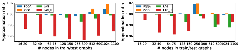
Figure 1: Approximation ratio comparison across different node sizes in train/test graphs.

5.4 Balanced Graph Partition

Table 5: Balanceness are Graph partition are evaluated on 5 benchmarks.

Metric	Methods	VGG	MNIST-conv	ResNet	AlexNet	Inception-v3
Edge cut ratio$\downarrow$	hMETIS	0.05	0.05	0.04	0.05	0.04
	GAP	0.04	0.05	0.04	0.04	0.04
	iSCO	0.05	0.04	0.05	0.05	0.05
	PQQA	0.04	0.04	0.03	0.04	0.03
Balanceness$\uparrow$	hMETIS	0.99	0.99	0.99	0.99	0.99
	GAP	0.99	0.99	0.99	0.99	0.99
	iSCO	0.99	0.99	0.99	0.99	0.99
	PQQA	0.99	0.99	0.99	0.99	0.99

We next demonstrate the results of applying PQQA to general discrete variables, using the generalization of entropy detailed in Appendix 18. Following Sun et al. (2023a); Nazi et al. (2019), PQQA is evaluated on balanced graph partition, including five different computation graphs from widely used deep neural networks. The largest graph, Inceptionv3 (Szegedy et al., 2017), consists of 27,144 nodes and 40,875 edges. The results are compared with iSCO, GAP (Nazi et al., 2019), which is a specialized learning architecture for graph partitioning, and hMETIS (Karypis and Kumar, 1999), a widely used framework for this problem. We use the edge cut ratio and balanceness for evaluation metrics, where a lower edge cut ratio indicates better performance, while a higher balanceness is preferable. Further details on these metrics and specific experimental conditions are provided in Appendix D.1. Table 5 shows that PQQA achieves better results with near-perfect balanceness and a lower cut ratio. Although PQQA required approximately 20 minutes for the largest graph, GAP, the fastest method, was completed in around 2 minutes. However, PQQA consistently achieved a lower edge cut ratio than GAP. Furthermore, with iSCO taking approximately 30 minutes to run, PQQA stands out as the faster approach, while still achieving a better edge cut ratio.

5.5 Graph Coloring

Table 6: Numerical results for COLOR graphs (Trick, 2002) are presented. For a specified number of colors, we report the cost, defined as the number of conflicts in the best coloring obtained by PQQA, PI-GCV, PI-SAGE (learning-based methods), and Tabucol (a tabu search-based method), sourced from Schuetz et al. (2022b); Yang et al. (2021).

Graph	Colors	Tabucol	GNN	PI-GCN	PI-SAGE	PQQA
anna	11	0	1	1	0	0
jean	10	0	0	0	0	0
myciel5	6	0	0	0	0	0
myciel6	7	0	0	0	0	0
queen5-5	5	0	0	0	0	0
queen6-6	7	0	4	1	0	0
queen7-7	7	0	15	8	0	0
queen8-8	9	0	7	6	1	0
queen9-9	10	0	13	13	1	0
queen8-12	12	0	7	10	0	0
queen11-11	11	20	33	37	17	11
queen13-13	13	35	40	61	26	14

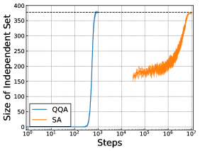
Figure 2: Comparison of SA and single-run QQA (S=1).

We evaluate PQQA on the graph coloring problem. Following the experimental setup of Schuetz et al. (2022b), we report the results on the publicly available COLOR dataset (Trick, 2002), commonly used in graph-based benchmark studies. For more detail on the dataset properties and specific experimental conditions, refer to Appendix D.1. The evaluation metric is the cost, representing the number of conflicts in the best coloring solution. We compare PQQA against PI-GCV and PI-SAGE (Schuetz et al., 2022b), both general-purpose unsupervised learning based solvers, and Tabucol (Yang et al., 2021), a tabu search-based heuristic that performs local search within a tabu list. As shown in Table 6 shows that PQQA achive the best results.

5.6 Ablation Study

Detail Comparison with SA.

We compare our method to classical SA with Gibbs sampling. Figure 2 shows the ApR curves for an MIS on the largest ERGs in Section 5.1 as a function of the number of sampling steps. The results are reported as the mean and standard deviation across five random seeds. This experiment excluded communication between parallel runs to isolate the impact of gradient-based transitions, i.e., $S=1$. The results demonstrate that QQA achieves a speedup of over $10^{4}$ times in the number of steps. Moreover, using gradient information improves the stability of the solution process.

Schedule Speed and Initial $\gamma$.

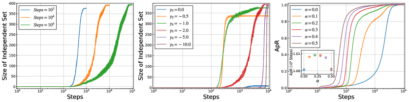
Figure 3: Ablation study on (left) annealing schedule speed, (middle) initial $\gamma$, and (right) communication strength $\alpha$. The shaded area denotes the standard deviation across five random seeds.

We conduct an ablation study to evaluate the impact of different $\gamma$ schedules and initial values, $\gamma_{0}$. As in SA, QQA with a smaller initial value $\gamma_{0}$ and slower annealing achieves better results. Thus, we examine how the solution quality varies across different parameter settings. For the MIS on the largest ER graph in Section 5.1, Figure 3 (left) shows the independent set size across various annealing speeds, with the initial $\gamma_{0}$ fixed at $-2$. The annealing follows a linear schedule determined by the maximum number of steps, where fewer steps correspond to faster annealing. The results show no performance degradation, even with faster annealing. Indeed, QQA with $10^{3}$ steps maintains an ApR around 1.00, outperforming other learning-based solvers. Figure 3 (middle) shows the results for different $\gamma_{0}$ values under the same annealing speed, indicating that skipping the annealing phase when $\gamma<0$ results in poor outcomes. Furthermore, the results are consistent when $\gamma_{0}$ is set below $-2$.

Communication Strength.

An important contribution of this study is the introduction of communication between parallel chains, which was not discussed in iSCO (Sun et al., 2023a). Here, we conduct an ablation study on the communication strength, $\alpha$ in Eq. (10). The number of parallel chains is set to $S=1{,}000$, and the performance is evaluated on the MIS on small ERGs, as described in Section 5.1 across various $\alpha$ values. Figure 3 shows the existence of the optimal $\alpha$ values, leading to the best ApR. Additionally, increasing $\alpha$ enhances convergence speed while maintaining performance comparable to the case of $\alpha=0$. This improvement arises from the effect of the STD term in Eq. (10), which implicitly drives the relaxed variables toward 0 or 1. Additional theoretical insights are detailed in Appendix A.2.

6 Conclusion

PQQA, which integrates QQA, gradient-based updates, and parallel run communication, demonstrates performance comparable to or superior to iSCO and learning-based solvers across various CO problems. Notably, for larger problems, PQQA achieves a superior speed-quality trade-off. This suggests that future research on learning-based methods should carefully evaluate their efficiency compared to our GPU-based, general-purpose approach. Future work includes extending PQQA to the mixed-integer optimization and sampling tasks.

Appendix A Derivation and Additional Theoretical Results

A.1 Derivation of Theorem 3.1

In this section, we present the proof of Theorem 3.1.

Theorem A.1.

Under the assumption that the objective function $\hat{l}({\bm{p}};C)$ is bounded within the domain $[0,1]^{N}$, the Boltzmann distribution $\lim_{\gamma\to+\infty}\lim_{T\to 0}\hat{P}(\sigma({\bm{w}});\gamma,T)$ converges to a uniform distribution over the optimal solutions of Eq. (2), i.e., ${\bm{x}}^{\ast}\in\mathrm{argmin}_{{\bm{x}}}l({\bm{x}};C,{\bm{\lambda}})$. Additionally, $\lim_{\gamma\to-\infty}\lim_{T\to 0}\hat{P}(\sigma({\bm{w}});\gamma,T)$ converges to a single-peaked distribution $\prod_{i=1}^{N}\delta(\sigma(w_{i})-\nicefrac{{1}}{{2}})$.

Proof.

We begin by recalling the definition of $\hat{P}(\sigma({\bm{w}});\gamma,T)$:

$$\hat{P}(\sigma({\bm{w}});\gamma,T)=\frac{1}{{\mathcal{Z}}(\gamma,T)}e^{-\frac{1}{T}\hat{r}(\sigma({\bm{w}});C,{\bm{\lambda}},\gamma)},~{}~{}{\mathcal{Z}}(\gamma,T)=\int\prod_{i=1}^{N}dw_{i}e^{-\frac{1}{T}\hat{r}(\sigma({\bm{w}});C,{\bm{\lambda}},\gamma)}.$$ (12)

where $\hat{r}(\sigma({\bm{w}});C,{\bm{\lambda}},\gamma)$ is defined as

$$\hat{r}(\sigma({\bm{w}});C,{\bm{\lambda}},\gamma)=\hat{l}(\sigma({\bm{w}});C,{\bm{\lambda}})+\gamma s(\sigma({\bm{w}})),$$ (13)

where $\gamma\in{\mathbb{R}}$ and $s(\sigma({\bm{w}}))$ is a convex function that takes its minimum value of $0$ when $\sigma({\bm{w}})\in\{0,1\}^{N}$ and a maximum value when $\sigma({\bm{w}})=\nicefrac{{{\bm{1}}_{N}}}{{2}}$. The set of global minimizers of $\hat{r}(\sigma({\bm{w}});C,{\bm{\lambda}},\gamma)$ is defined as:

$$\Omega^{\ast}_{\gamma}=\mathrm{argmin}_{{\bm{w}}\in{\mathbb{R}}^{N}}\hat{r}(\sigma({\bm{w}});C,{\bm{\lambda}},\gamma).$$

The remainder of the state space is denoted by $\Omega_{\gamma}={\mathbb{R}}^{N}\setminus\Omega^{\ast}_{\gamma}$. In the limit as $T\to+0$, the following holds:

$$\lim_{T\to+0}\hat{P}(\sigma({\bm{w}});\gamma,T) =\frac{e^{-\frac{1}{T}\hat{r}(\sigma({\bm{w}});C,{\bm{\lambda}},\gamma)}}{\int\prod_{i=1}^{N}dw_{i}e^{-\frac{1}{T}\hat{r}(\sigma({\bm{w}});C,{\bm{\lambda}},\gamma)}},$$

$$=\lim_{T\to+0}\frac{e^{\frac{1}{T}\left(\hat{r}(\sigma({\bm{w}}^{\ast});C,{\bm{\lambda}},\gamma)-\hat{r}(\sigma({\bm{w}});C,{\bm{\lambda}},\gamma)\right)}}{\int\prod_{i=1}^{N}dw_{i}e^{\frac{1}{T}\left(\hat{r}(\sigma({\bm{w}}^{\ast});C,{\bm{\lambda}},\gamma)-\hat{r}(\sigma({\bm{w}});C,{\bm{\lambda}},\gamma)\right)}}$$

$$=\lim_{T\to+0}\frac{1}{\int\prod_{i=1}^{N}dw_{i}e^{\frac{1}{T}\left(\hat{r}(\sigma({\bm{w}}^{\ast});C,{\bm{\lambda}},\gamma)-\hat{r}(\sigma({\bm{w}});C,{\bm{\lambda}},\gamma)\right)}}\delta({\bm{w}}-{\bm{w}}^{\ast})$$

$$+\lim_{T\to+0}\frac{e^{\frac{1}{T}\left(\hat{r}(\sigma(\hat{{\bm{w}}});C,{\bm{\lambda}},\gamma)-\hat{r}(\sigma({\bm{w}});C,{\bm{\lambda}},\gamma)\right)}}{\int\prod_{i=1}^{N}dw_{i}e^{\frac{1}{T}\left(\hat{r}(\sigma(\hat{{\bm{w}}});C,{\bm{\lambda}},\gamma)-\hat{r}(\sigma({\bm{w}});C,{\bm{\lambda}},\gamma)\right)}}\delta({\bm{w}}-\hat{{\bm{w}}})$$

$$=\lim_{T\to+0}\frac{1}{\int\prod_{i=1}^{N}dw_{i}\sum_{{\bm{w}}^{\ast}\in\Omega_{\gamma}^{\ast}}\delta({\bm{w}}-{\bm{w}}^{\ast})}\delta({\bm{w}}-{\bm{w}}^{\ast})$$

$$=\frac{1}{|\Omega_{\gamma}^{\ast}|}\delta({\bm{w}}-{\bm{w}}^{\ast}),$$

where ${\bm{w}}^{\ast}\in\Omega_{\gamma}^{\ast}$ and $\hat{{\bm{w}}}\in\Omega_{\gamma}$. Here, we applied the property that $\lim_{T\to+0}e^{\nicefrac{{x}}{{T}}}=1$ when $x=0$, and $\lim_{T\to+0}e^{\nicefrac{{x}}{{T}}}=0$ when $x<0$. Therefore, in the limit as $T\to+0$, the distribution $\hat{P}(\sigma({\bm{w}});\gamma,T)$ converges to a uniform distribution over the set of global minimizers $\Omega_{\gamma}^{\ast}$ of Eq. (13). Given that $s(\sigma({\bm{w}}))$ is a convex function with minimum value $0$ when $\sigma({\bm{w}})\in\{0,1\}^{N}$ and maximum value at $1/2$, in the limit as $\gamma\to+\infty$, the entropy term $s(\sigma({\bm{w}}))$ becomes dominant. Consequently, the state space is constrained to the set $\sigma({\bm{w}})\in\{0,1\}^{N}$ where $s(\sigma({\bm{w}}))=0$. Minimizing $\hat{l}(\sigma({\bm{w}});C,{\bm{\lambda}})$ within this constrained space yields:

$$\lim_{\gamma\to+\infty}\Omega_{\gamma}^{\ast}=\mathrm{argmin}_{{\bm{x}}\in\{0,1\}^{N}}l({\bm{x}};C,{\bm{\lambda}}).$$ (14)

Thus, in the limit as $\gamma\to\infty$ followed by $T\to+0$, $\hat{P}(\sigma({\bm{w}});\gamma,T)$ converges to a uniform distribution over the set of global minimizers of the discrete objective function $l({\bm{x}};C,{\bm{\lambda}})$. Conversely, as $\gamma\to-\infty$, the entropy $s(\sigma({\bm{w}}))$ reaches its maximum value when $\sigma({\bm{w}})=\nicefrac{{{\bm{1}}_{N}}}{{2}}$, leading to the minimization of $\hat{r}({\bm{w}};C,{\bm{\lambda}},\gamma)$ at $\Omega_{\gamma}^{\ast}=\{\nicefrac{{{\bm{1}}_{N}}}{{2}}\}$. Hence, we have:

$$\lim_{\gamma\to-\infty}\lim_{T\to+0}\hat{P}(\sigma({\bm{w}});\gamma,T)=\prod_{i=1}^{N}\delta(\sigma(w_{i})-\nicefrac{{1}}{{2}}).$$ (15)

This concludes the proof. ∎

A.2 Additional Theoretical Results

The following proposition holds for the communication term in Eq. (10).

Proposition A.2.

The function $\sum_{i=1}^{N}{\mathbb{S}}{\mathbb{T}}{\mathbb{D}}[\{\sigma(w_{i}^{(s)})\}_{s=1}^{S}]$ is maximized when, for any $i\in[N]$, the set $\{\sigma(w^{(s)}_{i})\}_{s=1}^{S}$ consists of $\nicefrac{{S}}{{2}}$ zeros and $\nicefrac{{S}}{{2}}$ ones.

Proof.

Consider the expression ${\mathbb{S}}{\mathbb{T}}{\mathbb{D}}[\{\sigma({\bm{w}}^{(s)})\}_{s=1}^{S}]$, which can be expanded as:

$$\sum_{i=1}^{N}{\mathbb{S}}{\mathbb{T}}{\mathbb{D}}[\{\sigma(w_{i}^{(s)})\}_{s=1}^{S}]=\sum_{i=1}^{N}\sqrt{\sum_{s=1}^{S}\left(\sigma(w_{i}^{(s)})-\frac{1}{S}\sum_{s=1}^{S}\sigma(w_{i}^{(s)})\right)^{2}}.$$

Thus, it suffices to solve the following maximization problem for any $i\in[N]$:

$$\max_{\{\sigma(w_{i}^{(s)})\}_{s=1}^{S}}\sum_{s=1}^{S}\left(\sigma(w_{i}^{(s)})-\frac{1}{S}\sum_{s=1}^{S}\sigma(w_{i}^{(s)})\right)^{2}.$$

This problem can be addressed using the method of Lagrange multipliers. Given that $\sigma({\bm{w}}^{(s)})\in[0,1]^{N}$, we define the Lagrangian as:

$${\mathcal{L}}(\{\sigma(w_{i}^{(s)}),\lambda_{s},\nu_{s}\}_{s=1}^{S})=\sum_{s=1}^{S}\left(\sigma(w_{i}^{(s)})-\frac{1}{S}\sum_{s^{\prime}=1}^{S}\sigma(w_{i}^{(s^{\prime})})\right)^{2}\\ +\sum_{s=1}^{S}\lambda_{s}(-\sigma(w_{i}^{(s)}))+\sum_{s=1}^{S}\nu_{s}(1-\sigma(w_{i}^{(s)})),$$

where $\lambda_{s}$ and $\nu_{s}$ are the Lagrange multipliers corresponding to the constraints $0\leq\sigma(w_{i}^{(s)})\leq 1$. The stationarity condition gives:

$$\frac{\partial{\mathcal{L}}(\{\sigma(w_{i}^{(s)}),\lambda_{s},\nu_{s}\}_{s=1}^{S})}{\partial\sigma(w_{i}^{(s)})} =2\left(\sigma(w_{i}^{(s)})-\frac{1}{S}\sum_{s^{\prime}=1}^{S}\sigma(w_{i}^{(s^{\prime})})\right)\left(1-\frac{1}{S}\right)$$

$$-\frac{2}{S}\sum_{t\neq s}\left(\sigma(w_{i}^{(t)})-\frac{1}{S}\sum_{s^{\prime}=1}^{S}\sigma(w_{i}^{(s^{\prime})})\right)-\lambda_{s}+\nu_{s}$$

$$=2\left(\sigma(w_{i}^{(s)})-\frac{1}{S}\sum_{s^{\prime}=1}^{S}\sigma(w_{i}^{(s^{\prime})})\right)-\lambda_{s}+\nu_{s}=0.$$

From dual feasibility, $\lambda_{s}\geq 0$ and $\nu_{s}\geq 0$ for any $s\in[S]$. Moreover, complementary slackness implies $\lambda_{s}\sigma(w_{i}^{(s)})=0$ and $\nu_{s}(\sigma(w_{i}^{(s)})-1)=0$ for any $s\in[S]$. Considering the case where $\sigma(w_{i}^{(s)})=0$, $\lambda_{s}>0$ due to complementary slackness, and hence $\sigma(w_{i}^{(s)})=0$. On the other hand, if $\sigma(w_{i}^{(s)})=1$, then $\nu_{s}>0$, again due to complementary slackness, which forces $\sigma(w_{i}^{(s)})=1$. For the intermediate case where $0<\sigma(w_{i}^{(s)})<1$, both $\lambda_{s}$ and $\nu_{s}$ must be zero, implying that $\sigma(w_{i}^{(s)})=\nicefrac{{\sum_{s^{\prime}}\sigma(w_{i}^{(s^{\prime})})}}{{S}}$. This means that all $\sigma(w_{i}^{(s)})$ are equal, leading to the variance being minimized to zero. To achieve the maximum variance, consider the scenario where $K$ out of $S$ variables are set to $0$ and the remaining $S-K$ variables are set to $1$. The variance is then computed as:

$$\sum_{s=1}^{S}\left(\sigma(w_{i}^{(s)})-\frac{1}{S}\sum_{s=1}^{S}\sigma(w_{i}^{(s)})\right)^{2} =\frac{K}{S}\cdot\left(0-\frac{K}{S}\right)^{2}+\frac{S-K}{S}\cdot\left(1-\frac{K}{S}\right)^{2}$$

$$=\frac{K(S-K)}{S^{2}}.$$

To maximize this quadratic function, differentiate with respect to $K$:

$$\frac{d}{dK}\left(\frac{K(S-K)}{S^{2}}\right)=\frac{S-2K}{S^{2}}.$$

Setting this derivative to zero yields $K=\nicefrac{{S}}{{2}}$. For even $S$, the maximum variance is:

$$\frac{K(S-K)}{S^{2}}=\frac{\left(\frac{S}{2}\right)\left(\frac{S}{2}\right)}{S^{2}}=\frac{1}{4}.$$

For odd $S$, $K$ is either $\lfloor\nicefrac{{S}}{{2}}\rfloor$ or $\lceil\nicefrac{{S}}{{2}}\rceil$. In both cases, the maximum variance is:

$$\frac{\lfloor\frac{S}{2}\rfloor\cdot\lceil\frac{S}{2}\rceil}{S^{2}}=\frac{(S-1)(S+1)}{4S^{2}}=\frac{S^{2}-1}{4S^{2}}.$$

As $S$ increases, the variance approaches $\nicefrac{{1}}{{4}}$, consistent with the even case. ∎

This result suggests that the communication term also favors binary values for $\sigma({\bm{w}})\in\{0,1\}^{N}$. Indeed, as shown in the ablation study in Figure 3 (right), increasing the strength of the communication term $\alpha$ accelerates convergence. This may be due to the communication term further reinforcing binary variables, in addition to the entropy term.

Appendix B Generalization to discrete optimization problems

In this section, we generalize PQQA, defined for binary optimization, to a general discrete optimization problem. Specifically, we consider the following optimization problem:

$$\min_{{\bm{x}}\in\{1,\ldots,K\}^{N}}l({\bm{x}};C,{\bm{\lambda}}),$$ (16)

where $C$ represents the characteristic parameters of the problem, and $\lambda$ denotes the penalty coefficients. In this case, each discrete variable is relaxed to output probabilities for each discrete value, denoted as $\sigma(W)$, where $W\in\mathbb{R}^{N\times K}$ and the function $\sigma$ satisfies $\sum_{k=1}^{K}\sigma(W_{ik})=1$ for all $i\in[N]$, with the softmax function being a typical choice for $\sigma$. We then introduce an entropy term as follows:

$$\min_{W\in\mathbb{R}^{N\times K}}l(\sigma(W);C,{\bm{\lambda}})+\gamma s_{K}(\sigma(W)),$$ (17)

where $\sigma(W)$ takes its maximum value of $\nicefrac{{1}}{{K}}$ for all $i\in[N]$ and $k\in[K]$, and for all $i\in[N]$, there exists a $k$ such that $\sigma(W_{ik})=1$ and $\sigma(W_{ik^{\prime}})=0$ for all $k^{\prime}\in[K]\setminus\{k\}$. For example, we can consider the following entropy, which generalizes the $\alpha$-entropy:

$$s_{K}(\sigma({\bm{w}}))=\sum_{i=1}^{N}\left\{1-\frac{1}{(K-1)((K-1)^{\alpha-1}+1)}\sum_{k=1}^{K}(K\sigma(W_{ik})-1)^{\alpha}\right\},~{}~{}~{}\alpha\in\{2n\mid n\in\mathbb{N}\}.$$ (18)

where $\gamma\in\mathbb{R}$ is a penalty parameter. This entropy has the following properties:

Proposition B.1.

The entropy defined in Eq. (18) is equivalent with Eq. (7) when $K=2$.

Proof.

When $K=2$, Eq. (18) can be written as

$$s_{2}(\sigma(W))=\sum_{i=1}^{N}\left\{1-\frac{1}{2}(2\sigma(W_{i1})-1)^{\alpha}-\frac{1}{2}(2\sigma(W_{i2})-1)^{\alpha}\right\}.$$

From the properties of $\sigma$, for any $i\in[N]$, we have $\sigma(W_{i1})=1-\sigma(W_{i2})$. Using this relationship, we can rewrite the expression as follows:

$$s_{2}\left(\{\sigma(W_{i1})\}_{i=1}^{N}\right) =\sum_{i=1}^{N}\left\{1-\frac{1+(-1)^{\alpha}}{2}(2\sigma(W_{i1})-1)^{\alpha}\right\}.$$

Finally, by noting that $\alpha\in\{2n\mid n\in\mathbb{N}\}$ and redefining ${\bm{w}}=(W_{i1})_{i=1}^{N}$, we obtain $s_{2}(\sigma({\bm{w}}))=s(\sigma({\bm{w}}))$. ∎

Next, we generalize the following general discrete optimization problem:

$$\min_{{\bm{x}}\in\{\alpha_{1},\ldots,\alpha_{K}\}}l({\bm{x}};C,{\bm{\lambda}}),$$ (19)

where ${\bm{\alpha}}=(\alpha_{k})_{k=1}^{K}\in\mathbb{R}^{K}$. When applying PQQA to this problem, we use one-hot encoding to express the probability of $\alpha_{k}$ occurring for each $i\in[N]$ as $\sigma(W_{ik})$, and relax the discrete variable $x_{i}$ as $x_{i}={\bm{\alpha}}^{\top}\sigma(W_{i:})$. To encode this with one-hot encoding, we also employ the entropy $s_{K}(\sigma(W))$ in Eq. (18). Moreover, PQQA can be generalized to mixed-integer optimization problems by adding the entropy term only to the integer variables.

Appendix C Additional Implementation details

C.1 Reasons for not using the sigmoid function

We provide an intuitive explanation for avoiding the use of the sigmoid function, $\sigma(x)=1/(1+e^{-x})$ when mapping $w$ to the range $[0,1]$. Given the characteristics of the sigmoid function, ${\bm{w}}$ tends to take on extremely large positive or small negative values when $\sigma({\bm{w}})$ is almost binary value. This makes it challenging for gradient-based methods to transition $w$ from very large positive values to very small negative values and vice versa once the variable approaches discrete values. Indeed, experimental results indicate that the sigmoid function performs less effectively than the clamp function. Further exploration of transformations tailored for CO beyond the clamp function remains for future research.

C.2 Annealing Schedule

We linearly increase $\gamma$ from $\gamma_{\min}$ to $\gamma_{\max}$ over the total steps. In general, we set $\gamma_{\min}=-2$ and $\gamma_{\max}=0.1$. For the Max Cut problem, $\gamma_{\min}=-20$ was used for larger graphs, while $\gamma_{\min}=-5$ was applied for the remaining graphs.

C.3 Configuration of Optimizer

The learning rate was set to an appropriate value from $\{1,0.1,0.01\}$, depending on the specific problem. The weight decay was fixed at $0.01$ and the temperature was fixed as $T=0.001$.

C.4 Transformation for general discrete variables

For discrete variables, each row $i\in[N]$ of the updated matrix $W\in{\mathbb{R}}^{N\times K}$ is transformed as follows:

$$\sigma(W_{ik})=\frac{\mathrm{Clamp}(W_{ik})}{\sum_{k^{\prime}=1}^{K}\mathrm{Clamp}(W_{ik^{\prime}})},~{}~{}\forall k\in[K].$$ (20)

Appendix D Additional Experiment Details

D.1 Energy Function of Benchmark Problems

In this section we provide the actual energy function we used for each of the problems we experimented in the main paper. For a graph $G=(V,E)$ we label the nodes in $V$ from $1$ to $N$. The adjacency matrix is represented as $A$. For a weighted graph we simply let $A_{ij}$ denote the edge weight between node $i$ and $j$. For constraint problems, we follow Sun et al. [2022] to select penalty coefficient $\lambda$ as the minimum value of $\lambda$ such that $x^{\ast}=\mathrm{argmin}_{x\in\{0,1\}^{N}}l({\bm{x}};{\bm{\lambda}},C)$ is achieved at ${\bm{x}}^{\ast}$ satisfying the original constraints. Such a choice of the coefficient guarantees the target distribution converges to the optimal solution of the original CO problems while keeping the target distribution as smooth as possible.

Max Independent Set.

The MIS problem is a fundamental NP-hard problem [Karp, 2010] defined as follows. Given an undirected graph $G(V,E)$, an independent set (IS) is a subset of nodes ${\mathcal{I}}\in V$ where any two nodes in the set are not adjacent. The MIS problem attempts to find the largest IS, which is denoted ${\mathcal{I}}^{\ast}$. In this study, $\rho$ denotes the IS density, where $\rho=|{\mathcal{I}}|/|V|$. To formulate the problem, a binary variable $x_{i}$ is assigned to each node $i\in V$. Then the MIS problem is formulated as follows:

$$\min_{{\bm{x}}\in\{0,1\}^{N}}-\sum_{i=1}^{N}c_{i}x_{i},~{}~{}\mathrm{s.t.}~{}x_{i}x_{j}=0,~{}~{}\forall(i,j)\in E.$$ (21)

We use the corresponding energy function in the following quadratic form:

$$l({\bm{x}};A,\lambda)=-{\bm{c}}^{\top}{\bm{x}}+\lambda\frac{{\bm{x}}^{\top}A{\bm{x}}}{2}.$$ (22)

where the first term attempts to maximize the number of nodes assigned $1$, and the second term penalizes the adjacent nodes marked $1$ according to the penalty parameter $\lambda$. In our experiments ${\bm{c}}={\bm{1}}_{N}$ and we use $\lambda=2$. First, for every $d$, a specific value $\rho_{d}^{\ast}$, which is dependent on only the degree $d$, exists such that the independent set density $|{\mathcal{I}}^{\ast}|/|V|$ converges to $\rho_{d}^{\ast}$ with a high probability as $N$ approaches infinity [Bayati et al., 2010]. Second, a statistical mechanical analysis provides the typical MIS density $\rho^{\mathrm{Theory}}_{d}$ and we clarify that for $d>16$, the solution space of ${\mathcal{I}}$ undergoes a clustering transition, which is associated with hardness in sampling [Barbier et al., 2013] because the clustering is likely to create relevant barriers that affect any algorithm searching for the MIS ${\mathcal{I}}^{\ast}$. Finally, the hardness is supported by analytical results in a large $d$ limit, which indicates that, while the maximum independent set density is known to have density $\rho^{\ast}_{d\to\infty}=2\log(d)/d$, to the best of our knowledge, there is no known algorithm that can find an independent set density exceeding $\rho^{\mathrm{alg}}_{d\to\infty}=\log(d)/d$ [Coja-Oghlan and Efthymiou, 2015].

Max Clique.

The max clique problem is equivalent to MIS on the dual graph. The max clique the integer programming formulation as

$$\min_{{\bm{x}}\in\{0,1\}^{N}}-\sum_{i=1}^{N}c_{i}x_{i},~{}~{}\mathrm{s.t.}~{}x_{i}x_{j}=0,~{}~{}\forall(i,j)\notin E.$$ (23)

The energy function is expressed as

$$l({\bm{x}};A,\lambda)=-{\bm{c}}^{\top}{\bm{x}}+\frac{\lambda}{2}\left({\bm{1}}_{N}^{\top}{\bm{x}}({\bm{1}}_{N}^{\top}{\bm{x}}-1)-{\bm{x}}^{\top}A{\bm{x}}\right),$$ (24)

where ${\bm{1}}_{N}$ denotes the vector $(1,\ldots,1)^{\top}\in{\mathbb{R}}^{N}$. In our experiments ${\bm{c}}={\bm{1}}_{N}$ and we use $\lambda=2$.

Max Cut.

The MaxCut problem is also a fundamental NP-hard problem [Karp, 2010] with practical application in machine scheduling [Alidaee et al., 1994], image recognition [Neven et al., 2008] and electronic circuit layout design [Deza and Laurent, 1994]. Given an graph $G=(V,E)$, a cut set ${\mathcal{C}}\in E$ is defined as a subset of the edge set between the node sets dividing $(V_{1},V_{2}\mid V_{1}\cup V_{2}=V,~{}V_{1}\cap V_{2}=\emptyset)$. The MaxCut problems aim to find the maximum cut set, denoted ${\mathcal{C}}^{\ast}$. Here, the cut ratio is defined as $\nu=|\mathcal{C}|/|\mathcal{V}|$, where $|\mathcal{C}|$ is the cardinality of the cut set. To formulate this problem, each node is assigned a binary variable, where $x_{i}=1$ indicates that node $i$ belongs to $V_{1}$, and $x_{i}=0$ indicates that the node belongs to $V_{2}$. Here, $x_{i}+x_{j}-2x_{i}x_{j}=1$ holds if the edge $(i,j)\in{\mathcal{C}}$. As a result, we obtain the following:

$$\min_{{\bm{x}}\in\{0,1\}^{N}}-\sum_{(i,j)\in E}A_{ij}\left(\frac{1-(2x_{i}-1)(2x_{j}-1)}{2}\right)$$ (25)

Due to no constraints on this problem, the energy function can be expressed as

$$l({\bm{x}};A)=-\sum_{(i,j)\in E}A_{ij}\left(\frac{1-(2x_{i}-1)(2x_{j}-1)}{2}\right).$$ (26)

Balanced Graph Partition.

The balanced graph partition is formulated as follows:

$$\min_{{\bm{x}}\in\{0,1,\ldots,k\}^{N}}\sum_{s=1}^{k}\sum_{(i,j)\in E}{\mathbb{I}}\left[x_{i}\neq x_{j}\&\&(x_{i}=s\|x_{j}=s)\right]+\lambda\sum_{s=1}^{k}\left(\frac{d}{k}-\sum_{i=1}^{N}{\mathbb{I}}(x_{i}=s)\right)^{2}$$ (27)

where $k$ is the number of partitions. The goal of graph partitioning is to achieve balanced partitions while minimizing the edge cut. The quality of the resulting partitions is assessed using the following metrics: (1) Edge cut ratio, defined as the ratio of edges across partitions to the total number of edges, and (2) Balancedness, calculated as one minus the difference between the number of nodes in each partition and the ideal partition size as follows:

$$\mathrm{Balanceness}=1-\sum_{s=1}^{k}\left(\frac{1}{k}-\frac{\sum_{i=1}^{d}{\mathbb{I}}(x_{i}=s)}{N}\right)^{2}.$$ (28)

Graph Coloring.

The graph coloring problem is formulated as follows:

$$\min_{{\bm{x}}\in\{0,1,\ldots,K\}^{N}}\left(-\sum_{(i,j)\in E}{\mathbb{I}}[x_{i}=x_{j}]\right)$$ (29)

where $K$ is a number of color. Following Schuetz et al. [2022b], we evaluate several benchmark instances from the COLOR dataset [Trick, 2002] for graph coloring. These instances can be categorized as follows:

• Book graphs: For a given work of literature, a graph is created with each node representing a character. Two nodes are connected by an edge if the corresponding characters encounter each other in the book. This type of graph is publicly available for Tolstoy’s Anna Karenina (anna), and Hugo0"80"99s.

• Myciel graphs: This family of graphs is based on the Mycielski transformation. The Myciel graphs are known to be difficult to solve because they are triangle free (clique number 2) but the coloring number increases in problem size.

• Queens graphs: This family of graphs is constructed as follows. Given an $n$ by $n$ chessboard, a queens graph is a graph made of $n^{2}$ nodes, each corresponding to a square of the board. Two nodes are then connected by an edge if the corresponding squares are in the same row, column, or diagonal. In other words, two nodes are adjacent if and only if queens placed on these two nodes can attack each other in a single move. In all cases, the maximum clique in the graph is no more than $n$, and the coloring value is lower-bounded by $n$.

Table 7: Synthetic data statistics.

	MIS		max clique	maxcut
Name	ER-[700-800]	ER-[9000-11000]	RB	ER	BA
# max nodes	800	10,915	475	1,100	1,100
# max edges	47,885	1,190,799	90,585	91,239	4,384
# instances	128	16	500	1,000	1,000

Table 8: Synthetic data statistics of graph coloring.

Graph	# nodes	# edges	colors
anna	138	493	11
jean	80	254	10
myciel5	47	236	6
myciel6	95	755	7
queen5-5	25	160	5
queen6-6	36	290	7
queen7-7	49	476	7
queen8-8	64	728	9
queen9-9	81	1056	10
queen8-12	96	1368	12
queen11-11	121	1980	11
queen13-13	169	3328	13

Table 9: Real-world data statistics.

	MIS	Max Clique	Maxcut	Balanced Graph Partition
Name	Satlib	Twitter	Optsicom	Mnist	Vgg	Alexnet	Resnet	Inception
# max nodes	1,347	247	125	414	1,325	798	20,586	27,114
# max edges	5,978	12,174	375	623	2,036	1,198	32,298	40,875
# instances	500	196	10	1	1	1	1	1

D.2 Benchmark Details

We present additional details on our experiments. First, Table 9 and Table 9 shows the statistics of the synthetic datasets, including the maximum number of nodes and edges per graph and the number of test instances. Table 9 provides the corresponding statistics for the real-world graphs.

Appendix E Additional Results

E.1 MIS

In this section, we present additional information in Table 10, including references for each method and the sizes of the maximum independent sets obtained, alongside the MIS results discussed in Table 1.

Table 10: ApR (size of independent set) and runtime are evaluated on three benchmarks provided by DIMES [Qiu et al., 2022]. The ApR is assessed relative to the results obtained by KaMIS. Runtime is reported as the total clock time, denoted in seconds (s), minutes (m), or hours (h). Methods that fail to produce results within 10 times the time limit of DIMES are marked as N/A.

Method	Type	SATLIB		ER-[700-800]		ER-[9000-11000]
		ApR (size)	Time	ApR (size)	Time	ApR (size)	Time
KaMIS	OR	1.000 (425.96)	37.58m	1.000 (44.87)	52.13m	1.000 (381.31)	7.6h
Gurobi	OR	1.000 (425.95)	26.00m	0.922 (41.38)	50.00m	N/A	N/A
Intel [Li et al., 2018]	SL+TS	N/A	N/A	0.865 (38.80)	20.00m	N/A	N/A
	SL+G	0.988 (420.66)	23.05m	0.777 (34.86)	6.06m	0.746 (284.63)	5.02m
DGL [Böther et al., 2022]	SL+TS	N/A	N/A	0.830 (37.26)	22.71m	N/A	N/A
LwD [Ahn et al., 2020]	RL+S	0.991 (422.22)	18.83	0.918 (41.17)	6.33m	0.907 (345.88)	7.56m
DIMES [Qiu et al., 2022]	RL+G	0.989 (421.24)	24.17m	0.852 (38.24)	6.12m	0.841 (320.50)	5.21m
	RL+S	0.994 (423.28)	20.26m	0.937 (42.06)	12.01m	0.873 (332.80)	12.51m
iSCO [Sun et al., 2023a]	fewer	0.995 (423.66)	5.85m	0.998 (44.77)	1.38m	0.990 (377.5)	9.38m
	more	0.996 (424.16)	15.27m	1.006 (45.15)	5.56m	1.008 (384.20)	1.25h
PQQA (Ours)	fewer	0.993 (423.018)	7.34m	1.004 (44.91)	44.72s	1.027 (391.50)	5.83m
	more	0.994 (423.57)	1.21h	1.005 (45.11)	7.10m	1.039 (396.06)	58.48m
	fewer	0.996 (424.06)	1.25h	1.007 (45.20)	6.82m	1.033 (393.94)	41.26m
	more	0.996 (424.44)	12.46h	1.009 (45.29)	1.14h	1.043 (397.75)	6.80h

References

- Papadimitriou and Steiglitz [1998] Christos H Papadimitriou and Kenneth Steiglitz. Combinatorial optimization: algorithms and complexity. Courier Corporation, 1998.
- Crama [1997] Yves Crama. Combinatorial optimization models for production scheduling in automated manufacturing systems. European Journal of Operational Research, 99(1):136–153, 1997.
- Kirkpatrick et al. [1983] Scott Kirkpatrick, C Daniel Gelatt Jr, and Mario P Vecchi. Optimization by simulated annealing. science, 220(4598):671–680, 1983.
- Metropolis et al. [1953] Nicholas Metropolis, Arianna W Rosenbluth, Marshall N Rosenbluth, Augusta H Teller, and Edward Teller. Equation of state calculations by fast computing machines. The journal of chemical physics, 21(6):1087–1092, 1953.
- Hastings [1970] W Keith Hastings. Monte carlo sampling methods using markov chains and their applications. 1970.
- Neal [1996] Radford M Neal. Sampling from multimodal distributions using tempered transitions. Statistics and computing, 6:353–366, 1996.
- Hukushima and Nemoto [1996] Koji Hukushima and Koji Nemoto. Exchange monte carlo method and application to spin glass simulations. Journal of the Physical Society of Japan, 65(6):1604–1608, 1996.
- Johnson et al. [1989] David S Johnson, Cecilia R Aragon, Lyle A McGeoch, and Catherine Schevon. Optimization by simulated annealing: An experimental evaluation; part i, graph partitioning. Operations research, 37(6):865–892, 1989.
- Johnson et al. [1991] David S Johnson, Cecilia R Aragon, Lyle A McGeoch, and Catherine Schevon. Optimization by simulated annealing: an experimental evaluation; part ii, graph coloring and number partitioning. Operations research, 39(3):378–406, 1991.
- Earl and Deem [2005] David J Earl and Michael W Deem. Parallel tempering: Theory, applications, and new perspectives. Physical Chemistry Chemical Physics, 7(23):3910–3916, 2005.
- Li et al. [2018] Zhuwen Li, Qifeng Chen, and Vladlen Koltun. Combinatorial optimization with graph convolutional networks and guided tree search. Advances in neural information processing systems, 31, 2018.
- Gasse et al. [2019] Maxime Gasse, Didier Chételat, Nicola Ferroni, Laurent Charlin, and Andrea Lodi. Exact combinatorial optimization with graph convolutional neural networks. Advances in neural information processing systems, 32, 2019.
- Gupta et al. [2020] Prateek Gupta, Maxime Gasse, Elias Khalil, Pawan Mudigonda, Andrea Lodi, and Yoshua Bengio. Hybrid models for learning to branch. Advances in neural information processing systems, 33:18087–18097, 2020.
- Khalil et al. [2017] Elias Khalil, Hanjun Dai, Yuyu Zhang, Bistra Dilkina, and Le Song. Learning combinatorial optimization algorithms over graphs. Advances in neural information processing systems, 30, 2017.
- Kool et al. [2018] Wouter Kool, Herke Van Hoof, and Max Welling. Attention, learn to solve routing problems! arXiv preprint arXiv:1803.08475, 2018.
- Chen and Tian [2019] Xinyun Chen and Yuandong Tian. Learning to perform local rewriting for combinatorial optimization. Advances in Neural Information Processing Systems, 32, 2019.
- Karalias and Loukas [2020] Nikolaos Karalias and Andreas Loukas. Erdos goes neural: an unsupervised learning framework for combinatorial optimization on graphs. Advances in Neural Information Processing Systems, 33:6659–6672, 2020.
- Wang et al. [2022] Haoyu Peter Wang, Nan Wu, Hang Yang, Cong Hao, and Pan Li. Unsupervised learning for combinatorial optimization with principled objective relaxation. Advances in Neural Information Processing Systems, 35:31444–31458, 2022.
- Wang and Li [2023] Haoyu Wang and Pan Li. Unsupervised learning for combinatorial optimization needs meta-learning. arXiv preprint arXiv:2301.03116, 2023.
- Schuetz et al. [2022a] Martin JA Schuetz, J Kyle Brubaker, and Helmut G Katzgraber. Combinatorial optimization with physics-inspired graph neural networks. Nature Machine Intelligence, 4(4):367–377, 2022a.
- Schuetz et al. [2022b] Martin JA Schuetz, J Kyle Brubaker, Zhihuai Zhu, and Helmut G Katzgraber. Graph coloring with physics-inspired graph neural networks. Physical Review Research, 4(4):043131, 2022b.
- Ichikawa [2023] Yuma Ichikawa. Controlling continuous relaxation for combinatorial optimization. arXiv preprint arXiv:2309.16965, 2023.
- Schuetz et al. [2023] Martin JA Schuetz, J Kyle Brubaker, and Helmut G Katzgraber. Reply to: Modern graph neural networks do worse than classical greedy algorithms in solving combinatorial optimization problems like maximum independent set. Nature Machine Intelligence, 5(1):32–34, 2023.
- Sun et al. [2023a] Haoran Sun, Katayoon Goshvadi, Azade Nova, Dale Schuurmans, and Hanjun Dai. Revisiting sampling for combinatorial optimization. In International Conference on Machine Learning, pages 32859–32874. PMLR, 2023a.
- Sun et al. [2023b] Haoran Sun, Hanjun Dai, Bo Dai, Haomin Zhou, and Dale Schuurmans. Discrete langevin samplers via wasserstein gradient flow. In International Conference on Artificial Intelligence and Statistics, pages 6290–6313. PMLR, 2023b.
- Kadowaki and Nishimori [1998] Tadashi Kadowaki and Hidetoshi Nishimori. Quantum annealing in the transverse ising model. Physical Review E, 58(5):5355, 1998.
- Geman and Geman [1984] Stuart Geman and Donald Geman. Stochastic relaxation, gibbs distributions, and the bayesian restoration of images. IEEE Transactions on pattern analysis and machine intelligence, (6):721–741, 1984.
- Černỳ [1985] Vladimír Černỳ. Thermodynamical approach to the traveling salesman problem: An efficient simulation algorithm. Journal of optimization theory and applications, 45:41–51, 1985.
- Ichikawa and Iwashita [2024] Yuma Ichikawa and Hiroaki Iwashita. Continuous tensor relaxation for finding diverse solutions in combinatorial optimization problems. arXiv preprint arXiv:2402.02190, 2024.
- Loshchilov and Hutter [2017] Ilya Loshchilov and Frank Hutter. Decoupled weight decay regularization. arXiv preprint arXiv:1711.05101, 2017.
- Angelini and Ricci-Tersenghi [2019] Maria Chiara Angelini and Federico Ricci-Tersenghi. Monte carlo algorithms are very effective in finding the largest independent set in sparse random graphs. Physical Review E, 100(1):013302, 2019.
- Wang et al. [2009] Chiaming Wang, Jeffrey D Hyman, Allon Percus, and Russel Caflisch. Parallel tempering for the traveling salesman problem. International Journal of Modern Physics C, 20(04):539–556, 2009.
- Chen and Ke [2004] Yuan-Lin Chen and YL Ke. Multi-objective var planning for large-scale power systems using projection-based two-layer simulated annealing algorithms. IEE Proceedings-Generation, Transmission and Distribution, 151(4):555–560, 2004.
- Jwo et al. [1995] W-S Jwo, C-W Liu, C-C Liu, and Y-T Hsiao. Hybrid expert system and simulated annealing approach to optimal reactive power planning. IEE Proceedings-Generation, Transmission and Distribution, 142(4):381–385, 1995.
- Seçkiner and Kurt [2007] Serap Ulusam Seçkiner and Mustafa Kurt. A simulated annealing approach to the solution of job rotation scheduling problems. Applied Mathematics and Computation, 188(1):31–45, 2007.
- Thompson and Dowsland [1998] Jonathan M Thompson and Kathryn A Dowsland. A robust simulated annealing based examination timetabling system. Computers & Operations Research, 25(7-8):637–648, 1998.
- Tavakkoli-Moghaddam et al. [2007] Reza Tavakkoli-Moghaddam, Nima Safaei, MMO Kah, and Masoud Rabbani. A new capacitated vehicle routing problem with split service for minimizing fleet cost by simulated annealing. Journal of the Franklin Institute, 344(5):406–425, 2007.
- Van Breedam [1995] Alex Van Breedam. Improvement heuristics for the vehicle routing problem based on simulated annealing. European Journal of Operational Research, 86(3):480–490, 1995.
- Zhang et al. [2012] Yichuan Zhang, Zoubin Ghahramani, Amos J Storkey, and Charles Sutton. Continuous relaxations for discrete hamiltonian monte carlo. Advances in Neural Information Processing Systems, 25, 2012.
- Pakman and Paninski [2013] Ari Pakman and Liam Paninski. Auxiliary-variable exact hamiltonian monte carlo samplers for binary distributions. Advances in neural information processing systems, 26, 2013.
- Mohasel Afshar and Domke [2015] Hadi Mohasel Afshar and Justin Domke. Reflection, refraction, and hamiltonian monte carlo. Advances in neural information processing systems, 28, 2015.
- Dinh et al. [2017] Vu Dinh, Arman Bilge, Cheng Zhang, and Frederick A Matsen IV. Probabilistic path hamiltonian monte carlo. In International Conference on Machine Learning, pages 1009–1018. PMLR, 2017.
- Nishimura et al. [2020] Akihiko Nishimura, David B Dunson, and Jianfeng Lu. Discontinuous hamiltonian monte carlo for discrete parameters and discontinuous likelihoods. Biometrika, 107(2):365–380, 2020.
- Zhang et al. [2022] Ruqi Zhang, Xingchao Liu, and Qiang Liu. A langevin-like sampler for discrete distributions. In International Conference on Machine Learning, pages 26375–26396. PMLR, 2022.
- Sun et al. [2021] Haoran Sun, Hanjun Dai, Wei Xia, and Arun Ramamurthy. Path auxiliary proposal for mcmc in discrete space. In International Conference on Learning Representations, 2021.
- Grathwohl et al. [2021] Will Grathwohl, Kevin Swersky, Milad Hashemi, David Duvenaud, and Chris Maddison. Oops i took a gradient: Scalable sampling for discrete distributions. In International Conference on Machine Learning, pages 3831–3841. PMLR, 2021.
- McNaughton et al. [2020] B McNaughton, MV Milošević, A Perali, and S Pilati. Boosting monte carlo simulations of spin glasses using autoregressive neural networks. Physical Review E, 101(5):053312, 2020.
- Ichikawa et al. [2022] Yuma Ichikawa, Akira Nakagawa, Hiromoto Masayuki, and Yuhei Umeda. Toward unlimited self-learning monte carlo with annealing process using vae’s implicit isometricity. arXiv preprint arXiv:2211.14024, 2022.
- Qiu et al. [2022] Ruizhong Qiu, Zhiqing Sun, and Yiming Yang. DIMES: A differentiable meta solver for combinatorial optimization problems. In Advances in Neural Information Processing Systems 35, 2022.
- Goshvadi et al. [2023] Katayoon Goshvadi, Haoran Sun, Xingchao Liu, Azade Nova, Ruqi Zhang, Will Grathwohl, Dale Schuurmans, and Hanjun Dai. Discs: A benchmark for discrete sampling. In A. Oh, T. Naumann, A. Globerson, K. Saenko, M. Hardt, and S. Levine, editors, Advances in Neural Information Processing Systems, volume 36, pages 79035–79066. Curran Associates, Inc., 2023. URL https://proceedings.neurips.cc/paper_files/paper/2023/file/f9ad87c1ebbae8a3555adb31dbcacf44-Paper-Datasets_and_Benchmarks.pdf.
- Hoos and Stützle [2000] Holger H Hoos and Thomas Stützle. Satlib: An online resource for research on sat. Sat, 2000:283–292, 2000.
- Lamm et al. [2016] Sebastian Lamm, Peter Sanders, Christian Schulz, Darren Strash, and Renato F Werneck. Finding near-optimal independent sets at scale. In 2016 Proceedings of the eighteenth workshop on algorithm engineering and experiments (ALENEX), pages 138–150. SIAM, 2016.
- Hespe et al. [2019] Demian Hespe, Christian Schulz, and Darren Strash. Scalable kernelization for maximum independent sets. Journal of Experimental Algorithmics (JEA), 24:1–22, 2019.
- Barbier et al. [2013] Jean Barbier, Florent Krzakala, Lenka Zdeborová, and Pan Zhang. The hard-core model on random graphs revisited. In Journal of Physics: Conference Series, volume 473, page 012021. IOP Publishing, 2013.
- Angelini and Ricci-Tersenghi [2023] Maria Chiara Angelini and Federico Ricci-Tersenghi. Modern graph neural networks do worse than classical greedy algorithms in solving combinatorial optimization problems like maximum independent set. Nature Machine Intelligence, 5(1):29–31, 2023.
- Xu et al. [2007] Ke Xu, Frédéric Boussemart, Fred Hemery, and Christophe Lecoutre. Random constraint satisfaction: Easy generation of hard (satisfiable) instances. Artificial intelligence, 171(8-9):514–534, 2007.
- Jure [2014] Leskovec Jure. Snap datasets: Stanford large network dataset collection. Retrieved December 2021 from http://snap. stanford. edu/data, 2014.
- Toenshoff et al. [2021] Jan Toenshoff, Martin Ritzert, Hinrikus Wolf, and Martin Grohe. Graph neural networks for maximum constraint satisfaction. Frontiers in artificial intelligence, 3:580607, 2021.
- Dai et al. [2021] Hanjun Dai, Xinshi Chen, Yu Li, Xin Gao, and Le Song. A framework for differentiable discovery of graph algorithms. 2021.
- Nazi et al. [2019] Azade Nazi, Will Hang, Anna Goldie, Sujith Ravi, and Azalia Mirhoseini. Gap: Generalizable approximate graph partitioning framework. arXiv preprint arXiv:1903.00614, 2019.
- Szegedy et al. [2017] Christian Szegedy, Sergey Ioffe, Vincent Vanhoucke, and Alexander Alemi. Inception-v4, inception-resnet and the impact of residual connections on learning. In Proceedings of the AAAI conference on artificial intelligence, volume 31, 2017.
- Karypis and Kumar [1999] George Karypis and Vipin Kumar. Multilevel k-way hypergraph partitioning. In Proceedings of the 36th annual ACM/IEEE design automation conference, pages 343–348, 1999.
- Trick [2002] M. Trick. COLOR Dataset, 2002. URL https://mat.tepper.cmu.edu/COLOR02/. Accessed: 2024-09-27.
- Yang et al. [2021] Han Yang, Kaili Ma, and James Cheng. Rethinking graph regularization for graph neural networks. In Proceedings of the AAAI Conference on Artificial Intelligence, volume 35, pages 4573–4581, 2021.
- Sun et al. [2022] Haoran Sun, Etash K Guha, and Hanjun Dai. Annealed training for combinatorial optimization on graphs. arXiv preprint arXiv:2207.11542, 2022.
- Karp [2010] Richard M Karp. Reducibility among combinatorial problems. Springer, 2010.
- Bayati et al. [2010] Mohsen Bayati, David Gamarnik, and Prasad Tetali. Combinatorial approach to the interpolation method and scaling limits in sparse random graphs. In Proceedings of the forty-second ACM symposium on Theory of computing, pages 105–114, 2010.
- Coja-Oghlan and Efthymiou [2015] Amin Coja-Oghlan and Charilaos Efthymiou. On independent sets in random graphs. Random Structures & Algorithms, 47(3):436–486, 2015.
- Alidaee et al. [1994] Bahram Alidaee, Gary A Kochenberger, and Ahmad Ahmadian. 0-1 quadratic programming approach for optimum solutions of two scheduling problems. International Journal of Systems Science, 25(2):401–408, 1994.
- Neven et al. [2008] Hartmut Neven, Geordie Rose, and William G Macready. Image recognition with an adiabatic quantum computer i. mapping to quadratic unconstrained binary optimization. arXiv preprint arXiv:0804.4457, 2008.
- Deza and Laurent [1994] Michel Deza and Monique Laurent. Applications of cut polyhedra\CJK@punctchar\CJK@uniPunct0"80"94ii. Journal of Computational and Applied Mathematics, 55(2):217–247, 1994.
- Böther et al. [2022] Maximilian Böther, Otto Kißig, Martin Taraz, Sarel Cohen, Karen Seidel, and Tobias Friedrich. What’s wrong with deep learning in tree search for combinatorial optimization. arXiv preprint arXiv:2201.10494, 2022.
- Ahn et al. [2020] Sungsoo Ahn, Younggyo Seo, and Jinwoo Shin. Learning what to defer for maximum independent sets. In International conference on machine learning, pages 134–144. PMLR, 2020.