Robust Clustering on High-Dimensional Data with Stochastic Quantization
Abstract
This paper addresses the limitations of traditional vector quantization (clustering) algorithms, particularly K-Means and its variant K-Means++, and explores the Stochastic Quantization (SQ) algorithm as a scalable alternative for high-dimensional unsupervised and semi-supervised learning problems. Some traditional clustering algorithms suffer from inefficient memory utilization during computation, necessitating the loading of all data samples into memory, which becomes impractical for large-scale datasets. While variants such as Mini-Batch K-Means partially mitigate this issue by reducing memory usage, they lack robust theoretical convergence guarantees due to the non-convex nature of clustering problems. In contrast, the Stochastic Quantization algorithm provides strong theoretical convergence guarantees, making it a robust alternative for clustering tasks. We demonstrate the computational efficiency and rapid convergence of the algorithm on an image classification problem with partially labeled data, comparing model accuracy across various ratios of labeled to unlabeled data. To address the challenge of high dimensionality, we trained Triplet Network to encode images into low-dimensional representations in a latent space, which serve as a basis for comparing the efficiency of both the Stochastic Quantization algorithm and traditional quantization algorithms. Furthermore, we enhance the algorithm’s convergence speed by introducing modifications with an adaptive learning rate.
Keywords:
stochastic quantization clustering algorithms stochastic gradient descent non-convex optimization deep metric learning data compression1 Introduction
Quantization and clustering are fundamental encoding techniques that provide compact representations of original data [17, 21, 49]. Clustering algorithms have emerged as prominent tools for unsupervised learning, with recent applications spanning diverse domains such as location-allocation problems [57], document classification [47, 58], and data compression [56].
In this context, we consider a random variable with values in Euclidean space and distribution , representing the original distribution. The encoded discrete distribution is parameterized by a set of atoms with corresponding probabilities . The optimal quantization problem aims to find the encoded distribution that minimizes the distance to the original distribution. This mathematical structure is analogous to the optimal clustering problem, where the objective is to determine the positions of cluster centers such that the sum of distances from each element to the nearest cluster center is minimized.
The K-Means algorithm, proposed by Lloyd [32], has been widely used for solving quantization and clustering problems, with numerous extensions [21]. Bottou and Bengio [6] interpreted the K-Means algorithm as an analogue of Newton’s method and proposed several stochastic gradient descent algorithms for solving optimal quantization and clustering problems. However, traditional clustering algorithms are limited by the requirement to load all training data into memory, rendering them non-scalable for large datasets. To address this limitation, Sculley [50] introduced the Mini-Batch K-Means algorithm, which utilizes only a small subset of possible values at each iteration.
The Stochastic Quantization algorithm reframes the clustering problem as a stochastic transportation problem [28, 29] by minimizing the distance between elements of the original distribution and atoms of the encoded discrete distribution . This approach employs Stochastic Gradient Descent (SGD) [13, 23, 48] to search for an optimal minimum, leveraging its computational efficiency in large-scale machine learning problems [7]. The use of stochastic approximation allows the algorithm to update parameters with only one element per iteration, ensuring memory efficiency without compromising convergence to the minimum [36].
This paper explores advanced modifications of the Stochastic Quantization algorithm, incorporating accelerated variants of SGD [35, 44, 55] and adaptive learning rate techniques [24, 53] to enhance convergence speed. Norkin et al. [41] provide a comprehensive comparison of various SGD variants, highlighting their respective advantages and limitations, while also offering convergence speed estimations.
Given that the optimal quantization problem is non-smooth and non-convex, specialized methods are required [16, 52, 60]. To validate its convergence, we apply the general theory of non-smooth, non-convex stochastic optimization [14, 15, 33]. While traditional clustering algorithms lack theoretical foundations for convergence guarantees and rely primarily on seeding techniques [3], stochastic optimization theory provides specific conditions for the local convergence of the Stochastic Quantization algorithm, which we supplement in this research.
This paper introduces a novel approach to address semi-supervised learning challenges on high-dimensional data by integrating the Stochastic Quantization algorithm with a deep learning model based on the Triplet Network architecture [19]. The proposed method encodes images into low-dimensional representations in the latent space, generating meaningful encoded features for the Stochastic Quantization algorithm. By employing the Triplet Network, this approach overcomes the limitations of quantization and clustering algorithms in high-dimensional spaces, such as visualization difficulties and decreased precision as the number of dimensions increases [26].
To illustrate the efficiency and scalability of the Stochastic Quantization algorithm, we conducted experiments on a semi-supervised image classification problem using partially labeled data from the MNIST dataset [31]. The Triplet Network is initially trained on the labeled portion of the dataset as a supervised learning model. Subsequently, the trained network is utilized to project the remaining unlabeled data onto the latent space, which serves as input for training the Stochastic Quantization algorithm. The performance of the proposed solution is evaluated using the F1-score metric [10] for multi-label classification across various ratios of labeled to unlabeled data.
2 Stochastic Quantization
Unlike traditional clustering methods that minimize the distance between each element of and the nearest center , Stochastic Quantization conceptualizes the feature set and cluster centers as discrete probability distributions. The Wasserstein (or Kantorovich–Rubinstein) distance is employed to minimize distortion between these distributions when representing a continuous distribution by a discrete one [28, 29]. Subsequent research [28, 40] has explored the application of quantization algorithms to solve optimal allocation problems for service centers, where each atom of the discrete distribution represents the location of facilities and customers, respectively.
Definition 1
[28]. Optimal quantization minimizes the weighted sum of distances between elements of the feature set and centers :
| (1) |
subject to constraints:
| (2) |
where are normalized supply volumes, are transportation volumes, is the norm defining the distance between elements in the objective function (1), is a common constraint set for variables , and .
In this research, we employ the Euclidean norm () as the distance metric, defined as . The choice of distance metric may vary depending on the problem domain. For instance, the cosine similarity function is utilized in text similarity tasks [4, 9], while Kolmogorov and Levy metrics are employed for probability and risk theory problems [28].
It is evident that in the optimal plan, all mass at point is transported to the nearest point . Consequently, problem (1)-(2) can be reduced to the following non-convex, non-smooth global stochastic optimization problem, with the objective function defined as:
| (3) |
where
| (4) |
Here, denotes the expected value over the random index that takes values with probabilities , respectively.
Lemma 1
In the global optimum of (2), all belong to the convex hull of elements in the feature set.
Proof
Assume, by contradiction, that there exists some . Consider the projection of onto and points , . We observe that . If for some , then
| (5) |
Thus, is not a local minimum of the objective function (4). Now, consider the case where for all . By assumption, for some . The vector satisfies , contradicting the assumption that is a minimum. This completes the proof.
For a continuous probability distribution , we can interpret the objective function (3) as a mathematical expectation in a stochastic optimization problem [13, 36, 41]:
| (6) |
with
| (7) |
where the random variable may have a multimodal continuous distribution. The empirical approximation of in (6) is:
| (8) |
where are independent, identically distributed initial samples of the random variable . If , is convex, and , then problem (3) is unimodal and reduces to a convex stochastic optimization problem:
| (9) |
However, for , the function is non-smooth and non-convex. In terms of [33, 38], is a random generalized differentiable function, its generalized gradient set can be calculated by the chain rule:
| (10) |
The expected value function (4) is also generalized differentiable, and the set is a generalized gradient set of the function [33, 38]. Vectors , are stochastic generalized gradients of the function .
These gradients can be utilized to find the optimal element in a feature set using Stochastic Gradient Descent (SGD) [13, 23, 41, 48]:
| (11) |
where is a learning rate parameter, and is the projection operator onto the set . The iterative process (2)-(11) for finding the optimal element is summarized in Algorithm 1. While SGD is an efficient local optimization algorithm, the ultimate task is to find global minima of (3). The research in [42] proposes a stochastic branch and bound method applicable to the optimization algorithm (11). The idea is to sequentially partition the initial problem into regions (with constraint set ) and use upper and lower bounds to refine partitions with the so-called interchanges relaxation to obtain lower bounds:
| (12) | |||||
The local convergence conditions of the stochastic generalized gradient method for solving problem (3) are determined in Theorem 2.1, with the proof provided in [14, 15].
Theorem 2.1
Assume that are independent sample points from the set taken with probabilities :
| (14) |
Let denote the set of values of on critical (stationary) points of problem (3), where and represents the normal cone to the set at point . If does not contain intervals and the sequence is bounded, then converges to a connected component of , and the sequence has a limit.
2.1 Adaptive Stochastic Quantization
The minimization of the objective function (3) is a non-smooth, non-convex, multiextremal, large-scale stochastic optimization problem. Although the parameter update recurrent sequence based on SGD (11) can converge under conditions (14), Qian et al. [46] demonstrated that the variance of gradient oscillations increases proportionally to the size of training samples:
| (15) |
where represents the variance over a set, is the averaged gradient value over a subset , and . These gradient oscillations reduce the algorithm’s stability and slow down the convergence speed. While strategies such as manually tuned learning rate , annealing schedules [48], or averaged gradient over a subset can improve convergence stability, the slow convergence speed in high-dimensional models [41] remains a significant drawback of the SGD algorithm.
Polyak [44] proposed the Momentum Gradient Descent (or the ”Heavy Ball Method”) as an alternative modification to the SGD by introducing an acceleration multiplier to the recurrent sequence (11), using a physical analogy of the motion of a body under the force of friction:
| (16) |
Nesterov [35, 55] further improved the modified recurrent sequence (16) by introducing an extrapolation step for parameter estimation (Nesterov Accelerated Gradient or NAG):
| (17) |
Although modifications (16) and (17) can improve convergence speed, they often encounter the vanishing gradient problem on sparse data [8]. The root cause is the fixed learning rate value, which performs equal updates for both significant and insignificant model parameters. Duchi et al. [12] address this issue by introducing an adaptive learning rate , where the hyperparameter value is normalized over the accumulated gradient value to increase the update for more significant parameters (AdaGrad):
| (18) |
where is a linear combination of accumulated gradients from previous iterations, and is a denominator smoothing term. While approach (18) solves the convergence issue on sparse data, it introduces the problem of uncontrollable vanishing of the learning rate with each iteration, i.e., . Tieleman et al. [53] proposed another approach (RMSProp) for accumulated gradient normalization using a moving average , which substitutes the denominator with a stochastic approximation of the expected value to control learning rate vanishing with an averaging multiplier .
Kingma et al. [24] introduced a further modification to (18) by adding adaptive estimation of the gradient value (ADAM):
| (19) |
where is the adaptive first moment (expected value) estimation, is the adaptive second moment (variance) estimation, and are averaging multipliers. It is important to note that the values and may be biased (i.e., the expected value of the parameter does not equal the value itself), which can cause unexpected behavior in the oscillation’s variance. The authors proposed corrected estimations for (2.1) as:
| (20) |
Norkin et al. [41] provide an overview of these adaptive parameter update strategies and present a detailed comparison of their convergence speed in various problem settings.
3 Traditional Clustering Model
The optimal clustering problem seeks to find cluster centers that minimize the sum of distances from each point to the nearest center. Lloyd’s K-Means algorithm [32] is a prominent method for solving quantization and clustering problems, with numerous extensions [21]. Bottou and Bengio [6] interpreted the K-Means algorithm as an analogue of Newton’s method and proposed several stochastic gradient descent algorithms for optimal clustering. These stochastic K-Means algorithms use only a subset of possible values or even a single element at each iteration.
Definition 2
[32]. K-Means iterative algorithm starts with the set of current cluster centers , the feature set is subdivided into non-intersecting groups : point belongs to group if
| (21) |
Denote the number of points in group , if , . Remark that and depend on . K-Means iteratively evaluates next cluster centers with the estimation:
| (22) |
We can represent these vectors as
| (23) | |||||
In [6] the form of K-Means algorithm (23) was connected to Newton’s step for solving at each iteration the smooth quadratic problem
| (24) |
with block diagonal Hessian and with diagonal number in block . Moreover, it is easy to see that (23) is the exact analytical solution of the unconstrained quadratic minimization problem (24) under fixed partition of the index set . In that paper it was also considered stochastic batch and online version of the stochastic gradient methods with learning rate for solving a sequence of problems (24) but without rigorous convergence analysis.
The initial positions of cluster centers are set either at random among or according the algorithm K-Means++ [3, 37]. With K-Means++ initialization strategy, the rate of convergence to local optimum is estimated to be , where - an optimal solution [3]. Assume initial cluster centers have already been chosen. The next center is sampled from the set with probabilities:
| (25) |
The next positions of the cluster centers for are calculated as in the original Lloyd algorithm [32], the expectation-maximization (EM) approach to K-Means algorithm. Consider problem for :
| (26) |
Given objective function (26) is a generalized differentiable function [38], and to find its optima we utilize a generalized gradient set is calculated by the chain rule:
| (27) |
And its some generalized gradient is the compound vector :
| (28) |
Sculley [50] addresses the limitation of Lloyd algorithm with update rule (26), highlighting that objective function calculation is expensive for large datasets, due to time complexity for a given feature set , where - dimensionality of each sample . The author proposed a solution by introducing a Mini-Batch K-Means modification to the Lloyd algorithm, where the set of points is subdivided into non-intersecting subsets , , such that if . Some may occur empty, for example, if
In this modifications the generalized gradients of function is , where:
| (29) |
The standard generalized gradient method for solving problem (26) takes on the form (for ):
| (30) |
Recent studies [52, 60] have examined stochastic K-Means algorithms as methods for solving corresponding non-convex, non-smooth stochastic optimization problems. However, the convergence properties of these algorithms lack rigorous validation. Let is the number of elements in at iteration . If we chose dependent on , namely, , then process (30) becomes identical to K-Means one (22). Here and can be rather large that does not guarantee convergence of (22). A more general choice can be with satisfying conditions (14) and thus .
3.1 Modifications of K-Means algorithm
Robust clustering model assumes solving problem (3), (4) with parameter . Such choice of parameter makes the quantization and clustering model more robust to outliers. However, then stochastic generalized gradients of the objective function should be calculated by formula (2) and the stochastic clustering algorithm takes form (11).
One also can consider a complement to the sequence (30) by the Cesàro trajectory averaging:
| (31) |
Conditions of convergence for this averaged sequence were studied in [33], in particular, they admit learning rate proportional to . A similar approach for K-Means generated sequences (22) aims to average sequence by the feature set size :
| (32) |
The standard K-Means algorithm requires finding the nearest cluster center to each point . This can be a time consuming operation in case of very large number . Moreover, points may be sampled sequentially from some continuous distribution and thus the sample can be potentially arbitrary large. The Stochastic Quantization algorithm (31) uses only one sampled point at each iteration and thus only one problem is solved at iteration . But one can use a batch of such points instead of the whole sample , .
4 Data Encoding with Triplet Network
Our proposed semi-supervised classification approach addresses a critical challenge in clustering high-dimensional data by integrating Contrastive Learning techniques [19, 22] with Stochastic Quantization. While the Stochastic Quantization algorithm (2) effectively mitigates scalability issues for large datasets, it remains susceptible to the ”curse of dimensionality,” a phenomenon common to clustering methods that rely on distance minimization (e.g., K-Means and K-Means++). Kriegel et al. [26] elucidated this phenomenon, demonstrating that the concept of distance loses its discriminative power in high-dimensional spaces. Specifically, the distinction between the nearest and farthest points becomes increasingly negligible:
| (33) |
Our study focuses on high-dimensional data in the form of partially labeled handwritten digit images [31]. However, it is important to note that this approach is not limited to image data and can be applied to other high-dimensional data types, such as text documents [47, 58]. While efficient dimensionality reduction algorithms like Principal Component Analysis (PCA) [1, 11] exist, they are primarily applicable to mapping data between two continuous spaces. In contrast, our objective necessitates an algorithm that learns similarity features from discrete datasets and projects them onto a metric space where similar elements are grouped into clusters, a process known as similarity learning.
Recent research [34, 54] has employed a Triplet Network architecture to learn features from high-dimensional discrete image data and encode them into low-dimensional representations in the latent space. The authors proposed a semi-supervised learning approach where the Triplet Network is trained on a labeled subset of data to encode them into latent representations in , and subsequently used to project the remaining unlabeled fraction onto the same latent space. This approach significantly reduces the time and labor required for data annotation without compromising accuracy.
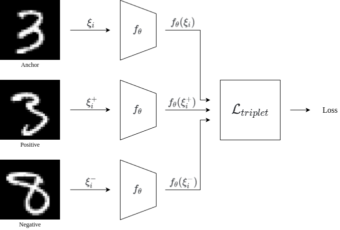
The Triplet Network, introduced by [19], is a modification of the Contrastive Learning framework [22]. Its core idea is to train the model using triplets of samples:
-
1.
An anchor sample : a randomly sampled element from the feature set
-
2.
A positive sample : an element with a label similar to the anchor
-
3.
A negative sample : an element with a label different from the anchor
Unlike traditional Contrastive Learning, which compares only positive and negative samples, the Triplet Network learns to minimize the distance between the anchor and positive samples while maximizing the distance between the anchor and negative samples. This is achieved using the triplet loss objective function (see Fig. 1):
| (34) |
where is a parameterized abstract operator mapping discrete elements into latent representations (in our case, a Triplet Network with weights ), is a distance metric between samples, and is a margin hyperparameter enforcing a minimum separation between positive and negative pairs. Analogous to the Stochastic Quantization distance metric (1), we employed the Euclidean norm for in (34).
In our research, we utilized a Convolutional Network architecture as , as proposed by [30]. The detailed overview of the architecture, its training using the Backpropagation algorithm, and accuracy evaluation are beyond the scope of this paper; [5], [27], and [30] provide extensive coverage of these topics. However, notice that function (34) is non-smooth and non-convex and the standard Backpropagation technique is not validated for such case. The extension of this technique to the non-smooth non-convex case was made in [39].
Regarding triplet mining strategies for , it is crucial to select an approach that produces the most informative gradients for the objective function (34). Paper [59] discusses various online triplet mining strategies, which select triplets within each batch of a training set on each iteration. We employed the semi-hard triplet mining strategy, which chooses an anchor-negative pair that is farther than the anchor-positive pair but within the margin :
| (35) |
where denotes the label of an element .
By applying ideas from [19, 34, 54], we can utilize the encoded latent representations of the Triplet Network to train a Stochastic Quantization (2) algorithm. This novel approach enables us to solve supervised or semi-supervised learning problems of classification on high-dimensional data. The semi-supervised learning process using the combined algorithm, assuming we have a labeled subset and remaining unlabeled data , can be summarized as follows:
-
1.
Train a Triplet Network on labeled data and produce encoded latent representations space
-
2.
Utilize the trained Triplet Network to project the remaining unlabeled data onto the same latent representation space
-
3.
Employ both labeled and unlabeled latent representations to train a Stochastic Quantization (2) algorithm
5 Numerical Experiments
To implement and train the Triplet Network, we utilized PyTorch 2.0 [2], a framework designed for high-performance parallel computations on accelerated hardware. The Stochastic Quantization algorithm was implemented using the high-level API of Scikit-learn [43], ensuring compatibility with other package components (e.g., model training and evaluation), while leveraging NumPy [18] for efficient tensor computations on CPU. All figures presented in this study were generated using Matplotlib [20]. The source code and experimental results are publicly available in our GitHub repository [25].
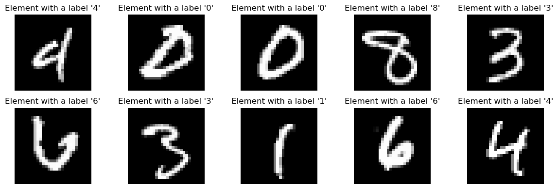
For our experiments, we employed the original MNIST handwritten digit dataset [31] (see Fig. 2), comprising 60,000 grayscale images of handwritten digits with a resolution of 28x28 pixels, each associated with a class label from 0 to 9. Additionally, the dataset includes a corresponding set of 10,000 test images with their respective labels. It is noteworthy that we did not apply any data augmentation or preprocessing techniques to either the training or test datasets.
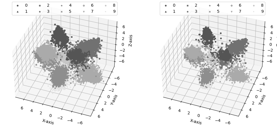
We approached the image classification task as a semi-supervised learning problem, training models on varying fractions of labeled training data (10%, 30%, 60%, 80%, and 100%). The training dataset was split using uniform sampling into labeled and unlabeled portions according to the specified percentages. For the Triplet Network, we employed a Convolutional Neural Network architecture consisting of two Convolutional Layers with 3x3 filters (feature map dimensions of 32 and 64, respectively, with and ), followed by 2x2 Max-Pooling layers, and two Dense Layers. ReLU (non-differentiable) activation functions were used throughout the network. Together with non-smooth Triplet loss function this makes the learning problem highly non-smooth and non-convex (see discussion of this issue in [39]). We trained separate Triplet Network models for each labeled data fraction with the following hyperparameters: 50 epochs, batch size of , learning rate , and regularization rate . For the triplet loss (34) and triplet mining (35), we set the margin hyperparameter . To facilitate meaningful feature capture while enabling visualization, we chose a latent space dimensionality of (see Fig. 3).
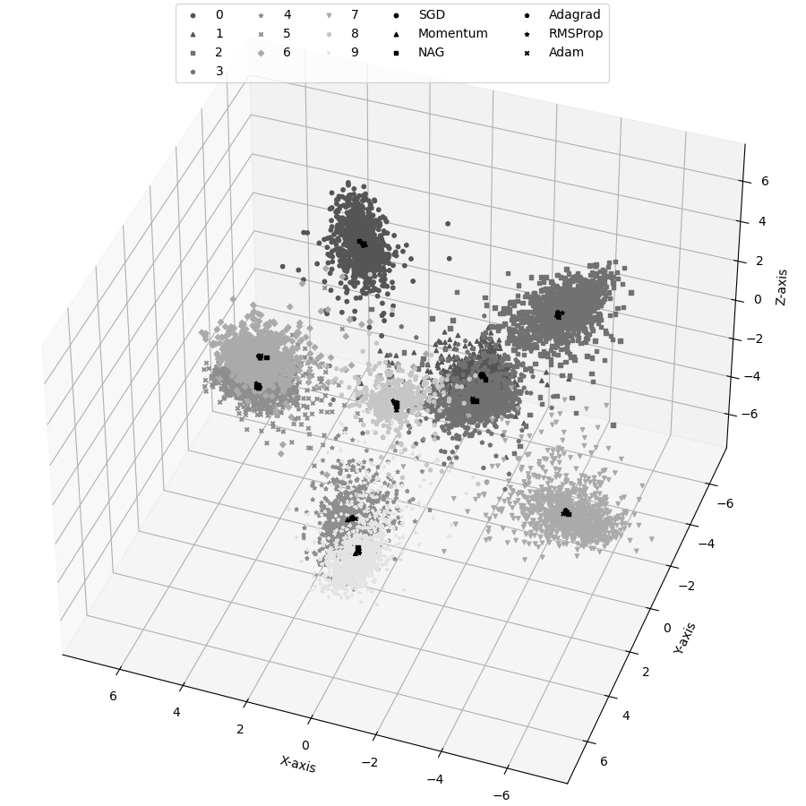
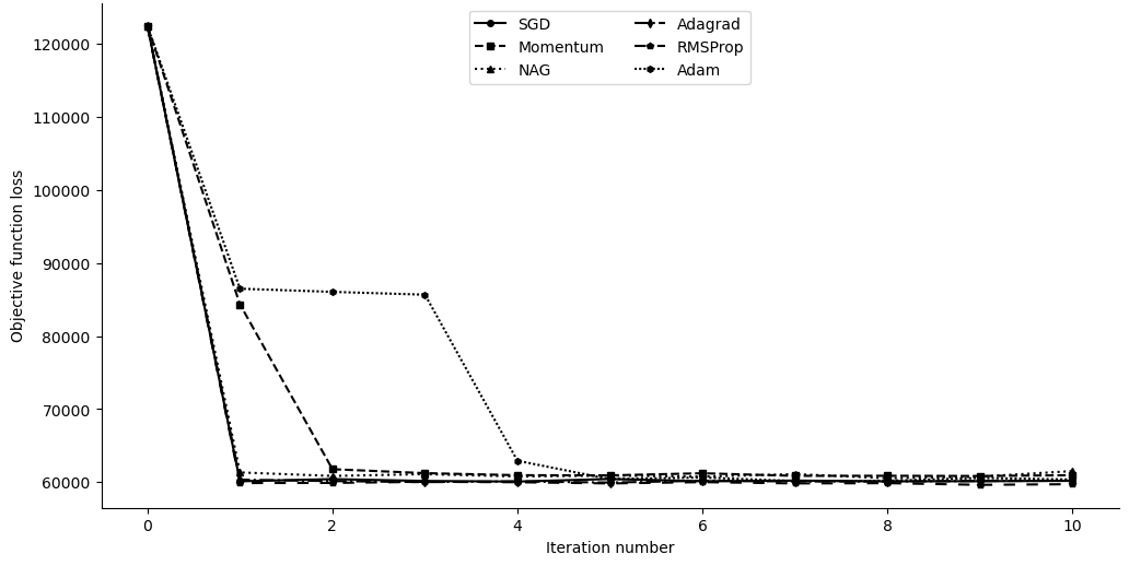
The Triplet Network was used to project latent representations onto space from both labeled and unlabeled training data. These representations were then used to train the Stochastic Quantization algorithm as an unsupervised learning model. For each set of latent representations corresponding to different labeled data fractions, we trained the Stochastic Quantization algorithm and its adaptive variants (16)–(2.1) from subsection 2.1. We employed the K-Means++ initialization strategy (25) for all variants, with a rank hyperparameter . To ensure convergence, we used different learning rates for each variant: for SGD, Momentum, and NAG; for AdaGrad; and for RMSProp and ADAM. With these hyperparameters, all Stochastic Quantization variants converged to the global optima (see Fig. 4), with most converging on the first iteration (see Fig. 5).
The accuracy of the trained classification models, combining Triplet Network and Stochastic Quantization, was evaluated using the F1-score metric [10] for weighted multi-label classification. Our experiments demonstrated that our approach achieved results comparable to state-of-the-art performance with Triplet Network and Siamese Network, as reported in [19], even with limited labeled data:
| Algorithm | Percentage of Training Data | ||||
|---|---|---|---|---|---|
| 10% | 30% | 60% | 80% | 100% | |
| Triplet Network + KNN | - | - | - | - | 99.54% |
| Siamese Network + KNN | - | - | - | - | 97.90% |
| Triplet Network + SQ-SGD | 94.67% | 98.14% | 98.23% | 98.17% | 98.26% |
| Triplet Network + SQ-Momentum | 92.97% | 98.20% | 98.26% | 98.14% | 98.24% |
| Triplet Network + SQ-NAG | 94.12% | 98.15% | 98.29% | 98.16% | 98.25% |
| Triplet Network + SQ-AdaGrad | 94.59% | 98.11% | 98.24% | 98.18% | 98.30% |
| Triplet Network + SQ-RMSProp | 94.34% | 98.16% | 98.19% | 98.17% | 98.27% |
| Triplet Network + SQ-ADAM | 93.01% | 98.18% | 98.23% | 98.18% | 98.25% |
6 Conclusions
In this paper, we introduced a novel approach to solving semi-supervised learning problems by combining Contrastive Learning with the Stochastic Quantization algorithm. Our robust solution addresses the challenge of scalability in large datasets for clustering problems, while also mitigating the ”curse of dimensionality” phenomenon through the integration of the Triplet Network. Although we introduced modifications to the Stochastic Quantization algorithm by incorporating an adaptive learning rate, there is potential for further enhancement by developing an alternative modification using the finite-difference algorithm proposed in [41], which will be the focus of future research. The semi-supervised nature of the problems addressed in this paper arises from the necessity of using labeled data to train the Triplet Network. By employing other Deep Neural Network architectures to produce low-dimensional representations in the latent space, the semi-supervised approach of Stochastic Quantization with Encoding could be extended to unsupervised learning. Additionally, alternative objective functions for contrastive learning, such as N-pair loss [51] or center loss [45], offer further avenues for exploration in future studies. The results obtained in this paper demonstrate that the proposed approach enables researchers to train classification models on high-dimensional, partially labeled data, significantly reducing the time and labor required for data annotation without substantially compromising accuracy.
References
- [1] Abdi, H., Williams, L.J.: Principal component analysis. WIREs Computational Statistics 2(4), 433–459 (Jul 2010). https://doi.org/10.1002/wics.101
- [2] Ansel, J., Yang, E., He, H., Gimelshein, N., Jain, A., Voznesensky, M., Bao, B., Bell, P., Berard, D., Burovski, E., et al.: Pytorch 2: Faster machine learning through dynamic python bytecode transformation and graph compilation. Proceedings of the 29th ACM International Conference on Architectural Support for Programming Languages and Operating Systems, Volume 2 (Apr 2024). https://doi.org/10.1145/3620665.3640366
- [3] Arthur, D., Vassilvitskii, S.: k-means++: the advantages of careful seeding. In: Proceedings of the Eighteenth Annual ACM-SIAM Symposium on Discrete Algorithms. p. 1027–1035. SODA ’07, Society for Industrial and Applied Mathematics, USA (2007)
- [4] Babić, K., Guerra, F., Martinčić-Ipšić, S., Meštrović, A.: A comparison of approaches for measuring the semantic similarity of short texts based on word embeddings. Journal of Information and Organizational Sciences 44(2) (Dec 2020). https://doi.org/10.31341/jios.44.2.2, //jios.foi.hr/index.php/jios/article/view/1427
- [5] Beohar, D., Rasool, A.: Handwritten digit recognition of mnist dataset using deep learning state-of-the-art artificial neural network (ann) and convolutional neural network (cnn). In: 2021 International Conference on Emerging Smart Computing and Informatics (ESCI). pp. 542–548 (2021). https://doi.org/10.1109/ESCI50559.2021.9396870
- [6] Bottou, L., Bengio, Y.: Convergence properties of the k-means algorithms. In: Tesauro, G., Touretzky, D.S., Leen, T.K. (eds.) Advances in Neural Information Processing Systems 7, [NIPS Conference, Denver, Colorado, USA, 1994]. pp. 585–592. MIT Press (1994)
- [7] Bottou, L.: Large-scale machine learning with stochastic gradient descent. Proceedings of COMPSTAT’2010 p. 177–186 (2010). https://doi.org/10.1007/978-3-7908-2604-3
- [8] Bottou, L., Curtis, F.E., Nocedal, J.: Optimization methods for large-scale machine learning. SIAM Review 60(2), 223–311 (2018). https://doi.org/10.1137/16m1080173
- [9] vor der Brück, T., Pouly, M.: Text similarity estimation based on word embeddings and matrix norms for targeted marketing. In: Burstein, J., Doran, C., Solorio, T. (eds.) Proceedings of the 2019 Conference of the North American Chapter of the Association for Computational Linguistics: Human Language Technologies, Volume 1 (Long and Short Papers). pp. 1827–1836. Association for Computational Linguistics, Minneapolis, Minnesota (Jun 2019). https://doi.org/10.18653/v1/N19-1181, https://aclanthology.org/N19-1181
- [10] Chinchor, N.: Muc-4 evaluation metrics. In: Proceedings of the 4th Conference on Message Understanding. p. 22–29. MUC4 ’92, Association for Computational Linguistics, USA (1992). https://doi.org/10.3115/1072064.1072067
- [11] Deisenroth, M.P., Faisal, A.A., Ong, C.S.: Dimensionality Reduction with Principal Component Analysis, p. 317–347. Cambridge University Press (2020)
- [12] Duchi, J., Hazan, E., Singer, Y.: Adaptive subgradient methods for online learning and stochastic optimization. J. Mach. Learn. Res. 12(null), 2121–2159 (jul 2011). https://doi.org/10.5555/1953048.2021068
- [13] Ermoliev, Y.: Stochastic Programming Methods. Nauka, Moscow (1976)
- [14] Ermoliev, Y.M., Norkin, V.I.: Solution of nonconvex nonsmooth stochastic optimization problems. Cybernetics and Systems Analysis 39(5), 701–715 (Sep 2003). https://doi.org/10.1023/b:casa.0000012091.84864.65
- [15] Ermol’ev, Y.M., Norkin, V.I.: Stochastic generalized gradient method for nonconvex nonsmooth stochastic optimization. Cybernetics and Systems Analysis 34(2), 196–215 (Mar 1998). https://doi.org/10.1007/bf02742069
- [16] Gandikota, V., Kane, D., Maity, R.K., Mazumdar, A.: Vqsgd: Vector quantized stochastic gradient descent. IEEE Transactions on Information Theory 68(7), 4573–4587 (Jul 2022). https://doi.org/10.1109/tit.2022.3161620
- [17] Graf, S., Luschgy, H.: Foundations of quantization for probability distributions. Lecture Notes in Mathematics 1730(1) (2000). https://doi.org/10.1007/bfb0103945
- [18] Harris, C.R., Millman, K.J., van der Walt, S.J., Gommers, R., Virtanen, P., Cournapeau, D., Wieser, E., Taylor, J., Berg, S., Smith, N.J., Kern, R., Picus, M., Hoyer, S., van Kerkwijk, M.H., Brett, M., Haldane, A., del Río, J.F., Wiebe, M., Peterson, P., Gérard-Marchant, P., Sheppard, K., Reddy, T., Weckesser, W., Abbasi, H., Gohlke, C., Oliphant, T.E.: Array programming with NumPy. Nature 585(7825), 357–362 (Sep 2020). https://doi.org/10.1038/s41586-020-2649-2
- [19] Hoffer, E., Ailon, N.: Deep metric learning using triplet network. In: Feragen, A., Pelillo, M., Loog, M. (eds.) Similarity-Based Pattern Recognition. pp. 84–92. Springer International Publishing, Cham (2015)
- [20] Hunter, J.D.: Matplotlib: A 2d graphics environment. Computing in Science & Engineering 9(3), 90–95 (2007). https://doi.org/10.1109/MCSE.2007.55
- [21] Jain, A.K.: Data clustering: 50 years beyond k-means. Pattern Recognition Letters 31(8), 651–666 (Jun 2010). https://doi.org/10.1016/j.patrec.2009.09.011
- [22] Khosla, P., Teterwak, P., Wang, C., Sarna, A., Tian, Y., Isola, P., Maschinot, A., Liu, C., Krishnan, D.: Supervised contrastive learning. In: Proceedings of the 34th International Conference on Neural Information Processing Systems. NIPS ’20, Curran Associates Inc., Red Hook, NY, USA (2020)
- [23] Kiefer, J., Wolfowitz, J.: Stochastic estimation of the maximum of a regression function. The Annals of Mathematical Statistics pp. 462–466 (1952)
- [24] Kingma, D.P., Ba, J.: Adam: A method for stochastic optimization (2017)
- [25] Kozyriev, A.: kaydotdev/stochastic-quantization: Robust clustering on high-dimensional data with stochastic quantization (Aug 2024), https://github.com/kaydotdev/stochastic-quantization
- [26] Kriegel, H.P., Kröger, P., Zimek, A.: Clustering high-dimensional data. ACM Transactions on Knowledge Discovery from Data 3(1), 1–58 (Mar 2009). https://doi.org/10.1145/1497577.1497578
- [27] Krizhevsky, A., Sutskever, I., Hinton, G.E.: Imagenet classification with deep convolutional neural networks. In: Proceedings of the 25th International Conference on Neural Information Processing Systems - Volume 1. p. 1097–1105. NIPS’12, Curran Associates Inc., Red Hook, NY, USA (2012). https://doi.org/10.5555/2999134.2999257
- [28] Kuzmenko, V., Uryasev, S.: Kantorovich–rubinstein distance minimization: Application to location problems. Springer Optimization and Its Applications 149, 59–68 (Sep 2019). https://doi.org/10.1007/978-3-030-22788-3_3
- [29] Lakshmanan, R., Pichler, A.: Soft quantization using entropic regularization. Entropy 25(10), 1435 (Oct 2023). https://doi.org/10.3390/e25101435
- [30] Lecun, Y., Bottou, L., Bengio, Y., Haffner, P.: Gradient-based learning applied to document recognition. Proceedings of the IEEE 86(11), 2278–2324 (1998). https://doi.org/10.1109/5.726791
- [31] LeCun, Y., Cortes, C., Burges, C.: Mnist handwritten digit database. ATT Labs [Online]. Available: http://yann.lecun.com/exdb/mnist 2 (2010)
- [32] Lloyd, S.: Least squares quantization in pcm. IEEE Transactions on Information Theory 28(2), 129–137 (Mar 1982). https://doi.org/10.1109/tit.1982.1056489
- [33] Mikhalevich, V.S., Gupal, A.M., Norkin, V.I.: Methods of nonconvex optimization (2024), https://arxiv.org/abs/2406.10406
- [34] Murasaki, K., Ando, S., Shimamura, J.: Semi-supervised representation learning via triplet loss based on explicit class ratio of unlabeled data. IEICE Transactions on Information and Systems E105.D(4), 778–784 (Apr 2022). https://doi.org/10.1587/transinf.2021edp7073
- [35] Nesterov, Y.E.: A method of solving a convex programming problem with convergence rate . In: Doklady Akademii Nauk. vol. 269, pp. 543–547. Russian Academy of Sciences (1983)
- [36] Newton, D., Yousefian, F., Pasupathy, R.: Stochastic gradient descent: Recent trends. Recent Advances in Optimization and Modeling of Contemporary Problems p. 193–220 (Oct 2018). https://doi.org/10.1287/educ.2018.0191
- [37] Nguyen, C.D., Duong, T.H.: K-means** - a fast and efficient k-means algorithms. International Journal of Intelligent Information and Database Systems 11(1), 27 (2018). https://doi.org/10.1504/ijiids.2018.091595
- [38] Norkin, V.I.: Stochastic generalized-differentiable functions in the problem of nonconvex nonsmooth stochastic optimization. Cybernetics 22(6), 804–809 (1986). https://doi.org/10.1007/bf01068698
- [39] Norkin, V.I.: Stochastic generalized gradient methods for training nonconvex nonsmooth neural networks. Cybernetics and Systems Analysis 57(5), 714–729 (2021). https://doi.org/10.984 1007/s10559-021-00397-z
- [40] Norkin, V.I., Onishchenko, B.O.: Minorant methods of stochastic global optimization. Cybernetics and Systems Analysis 41(2), 203–214 (Mar 2005). https://doi.org/10.1007/s10559-005-0053-4
- [41] Norkin, V., Kozyriev, A., Norkin, B.: Modern stochastic quasi-gradient optimization algorithms. International Scientific Technical Journal ”Problems of Control and Informatics” 69(2), 71–83 (Mar 2024). https://doi.org/10.34229/1028-0979-2024-2-6, https://jais.net.ua/index.php/files/article/view/228
- [42] Norkin, V.I., Pflug, G.C., Ruszczyński, A.: A branch and bound method for stochastic global optimization. Mathematical Programming 83(1–3), 425–450 (Jan 1998). https://doi.org/10.1007/bf02680569
- [43] Pedregosa, F., Varoquaux, G., Gramfort, A., Michel, V., Thirion, B., Grisel, O., Blondel, M., Prettenhofer, P., Weiss, R., Dubourg, V., Vanderplas, J., Passos, A., Cournapeau, D., Brucher, M., Perrot, M., Duchesnay, E.: Scikit-learn: Machine learning in Python. Journal of Machine Learning Research 12, 2825–2830 (2011)
- [44] Poliak, B.T.: The Heavy Ball Method, p. 65–68. Optimization Software (1987)
- [45] Qi, C., Su, F.: Contrastive-center loss for deep neural networks (2017), https://arxiv.org/abs/1707.07391
- [46] Qian, X., Klabjan, D.: The impact of the mini-batch size on the variance of gradients in stochastic gradient descent (2020), https://arxiv.org/abs/2004.13146
- [47] Radomirović, B., Jovanović, V., Nikolić, B., Stojanović, S., Venkatachalam, K., Zivkovic, M., Njeguš, A., Bacanin, N., Strumberger, I.: Text document clustering approach by improved sine cosine algorithm. Information Technology and Control 52(2), 541–561 (Jul 2023). https://doi.org/10.5755/j01.itc.52.2.33536
- [48] Robbins, H., Monro, S.: A stochastic approximation method. The Annals of Mathematical Statistics 22(3), 400–407 (1951). https://doi.org/10.1214/aoms/1177729586
- [49] Schölkopf, B., Smola, A.J.: Learning with Kernels: Support Vector Machines, Regularization, Optimization, and Beyond. MIT Press (2002)
- [50] Sculley, D.: Web-scale k-means clustering. Proceedings of the 19th international conference on World wide web p. 1177–1178 (Apr 2010). https://doi.org/10.1145/1772690.1772862
- [51] Sohn, K.: Improved deep metric learning with multi-class n-pair loss objective. In: Lee, D., Sugiyama, M., Luxburg, U., Guyon, I., Garnett, R. (eds.) Advances in Neural Information Processing Systems. vol. 29. Curran Associates, Inc. (2016)
- [52] Tang, C., Monteleoni, C.: Convergence rate of stochastic k-means. In: Singh, A., Zhu, J. (eds.) Proceedings of the 20th International Conference on Artificial Intelligence and Statistics. Proceedings of Machine Learning Research, vol. 54, pp. 1495–1503 (20–22 Apr 2017)
- [53] Tieleman, T., Hinton, G.: Rmsprop: Divide the gradient by a running average of its recent magnitude. coursera: Neural networks for machine learning. COURSERA Neural Networks Mach. Learn 17 (2012)
- [54] Turpault, N., Serizel, R., Vincent, E.: Semi-supervised triplet loss based learning of ambient audio embeddings. ICASSP 2019 - 2019 IEEE International Conference on Acoustics, Speech and Signal Processing (ICASSP) (May 2019). https://doi.org/10.1109/icassp.2019.8683774
- [55] Walkington, N.J.: Nesterov’s method for convex optimization. SIAM Review 65(2), 539–562 (2023). https://doi.org/10.1137/21M1390037
- [56] Wan, X.: Application of k-means algorithm in image compression. IOP Conference Series: Materials Science and Engineering 563(5) (Jul 2019). https://doi.org/10.1088/1757-899x/563/5/052042
- [57] Wang, M., Wei, X.: Research on logistics center location-allocation problem based on two-stage k-means algorithms. Advances in Intelligent Systems and Computing p. 52–62 (Aug 2020). https://doi.org/10.1007/978-3-030-55506-1_5
- [58] Widodo, A., Budi, I.: Clustering patent document in the field of ict (information & communication technology). In: 2011 International Conference on Semantic Technology and Information Retrieval. pp. 203–208 (2011). https://doi.org/10.1109/STAIR.2011.5995789
- [59] Xuan, H., Stylianou, A., Pless, R.: Improved embeddings with easy positive triplet mining (2020), https://arxiv.org/abs/1904.04370
- [60] Zhao, W.L., Lan, S.Y., Chen, R.Q., Ngo, C.W.: K-sums clustering. Proceedings of the 30th ACM International Conference on Information & Knowledge Management (Oct 2021). https://doi.org/10.1145/3459637.3482359