2D additive small-world network with distance-dependent interactions

Abstract

In this work, we have employed Monte Carlo calculations to study the Ising model on a 2D additive small-world network with long-range interactions depending on the geometric distance between interacting sites. The network is initially defined by a regular square lattice and with probability $p$ each site is tested for the possibility of creating a long-range interaction with any other site that has not yet received one. Here, we used the specific case where $p=1$, meaning that every site in the network has one long-range interaction in addition to the short-range interactions of the regular lattice. These long-range interactions depend on a power-law form, $J_{ij}=r_{ij}^{-\alpha}$, with the geometric distance $r_{ij}$ between connected sites $i$ and $j$. In current two-dimensional model, we found that mean-field critical behavior is observed only at $\alpha=0$. As $\alpha$ increases, the network size influences the phase transition point of the system, i.e., indicating a crossover behavior. However, given the two-dimensional system, we found the critical behavior of the short-range interaction at $\alpha\approx 2$. Thus, the limitation in the number of long-range interactions compared to the globally coupled model, as well as the form of the decay of these interactions, prevented us from finding a regime with finite phase transition points and continuously varying critical exponents in $0<\alpha<2$.

I Introduction

The small-world network model emerges as a proposal to capture the properties observed in Milgram’s social experiment [1]. In this 1967 experiment, it was found that any person can contact another with an average of only six intermediaries. Accordingly, a network that encompasses these properties should have a small average separation between nodes, compared to the maximum network lenght, as well as a high local clustering, given the nature of social networks. Two main network models reproduce these characteristics: the rewired small-world network (R-SWN) [2] and the additive small-world network (A-SWN) [3]. In the first case, we start with a regular network, each node is visited, and with probability $p$, the edges are randomly rewired, keeping the visited node as one of the endpoints of the edge. In the case A-SWN, we also start with a regular network, each node is visited, but with probability $p$, a random edge is created connecting the visited node with any other node in the network. The difference between the models lies in the greater simplicity of the A-SWN to implement and guarantee the small-world phenomenon for a wide range of $p$, i.e., $p\geq 1/N$ with $N$ being the number of nodes in the network. On the other hand, the R-SWN only maintains the small-world properties, more specifically the high local clustering, at low values of $p$.

A generalization of the Ising model [4] can be made by considering a globally coupled network, which has $N(N-1)/2$ distinct edges. In this context, the sites of this network are described as magnetic moments that can take only two values, $\sigma=\pm 1$, and the edges are interpreted as interactions between these magnetic moments, which can decay with the geometric distance, $r_{ij}$, between connected sites $i$ and $j$, with $J_{ij}=r_{ij}^{-\alpha}$. In this generalization, the critical behavior of the system depends on $\alpha$, with three regimes expected [5, 6]: (i) mean-field critical exponents for $0<\alpha<\alpha_{1}$; (ii) continuously varying critical exponents for $\alpha_{1}<\alpha<\alpha_{2}$; and (iii) critical exponents of the model with only short-range interactions for $\alpha>\alpha_{2}$. Both approximate analytical results and computational simulations show that $\alpha_{1}=3d/2$ and $\alpha_{2}\approx d+2$, with $d$ being the dimension of the network in question.

In this context, even with a wide range of complex networks already studied in physical systems [7, 8, 9, 10], there remains an open interest in verifying whether the long-range interactions present in the small-world network also affect the critical behavior of the Ising model if they depend on the distance between the sites in the network. The homogeneous interaction model, where $J_{ij}=1$ for any $r_{ij}$, reveals the critical behavior described by the critical exponents of the mean-field approximation, both in one [11] and two dimensions [12, 13]. However, by implementing spatial dependence in $J_{ij}$, the Ising model on the A-SWN in one dimension [14] only exhibited mean-field critical exponents at $\alpha=0$, resulting in $\alpha_{1}=\alpha_{2}=0$, because for $\alpha>0$, the long-range interactions did not significantly contribute to maintaining the system ordered in the thermodynamic limit. This resulted in a crossover behavior, where magnetic disorder is reached for any $\alpha>0$ when using sufficiently large networks.

Thus, in the present work, we aim to investigate the critical behavior of the Ising model on a 2D A-SWN, where the long-range interactions depend on the geometric distance between connected sites. This is because the 2D model on a regular lattice exhibits spontaneous magnetization at $T>0$, which consequently suggests the possibility of finding the three regimes predicted in the globally coupled model, with $\alpha_{1}\neq\alpha_{2}\neq 0$. To this end, we limit ourselves to the case of $p=1$, where every site in the network of size $N=L^{2}$ will have a long-range interaction that depends on the distance between connected sites according to $J_{ij}=r_{ij}^{-\alpha}$.

This article is organized as follows: In Section II, we present the network, and the dynamic involved in the system. We also provide details about the Monte Carlo method (MC), the thermodynamic quantities of interest, and the scaling relations for each of them. The results are discussed in Section III. And in Section IV, we present the conclusions drawn from the study.

II Model and Method

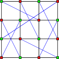
Figure 1: Schematic representation of the network used throughout the work, with $L=4$ and $N=16$. The black lines indicate short-range interactions between nearest neighbors sites on the regular lattice, with interaction strength $J=1$, and the blue dotted line indicates the long-range interactions added to the network, with interaction strength $J_{ij}=r_{ij}^{-\alpha}$. The green squares represent one of the sublattice sites, while the red squares represent the other sublattice sites, such that the long-range interactions connect the two sublattice sites.

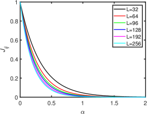
Figure 2: Behavior of $J_{ij}$ as a function of $\alpha$ for different network sizes, as shown in the figure. The interaction strength $J_{ij}$ is measured for sites that are separated by a distance equal to half the maximum distance between two sites on the network, i.e., $r_{ij}=\sqrt{2L^{2}}/2$.

In the ferromagnetic Ising model on the 2D A-SWN, the interaction energy between spins is defined by the Hamiltonian in the following form:

$$\mathcal{H}=-\sum_{\left\langle i,j\right\rangle}J\sigma_{i}\sigma_{j}-\sum_{i}J_{ij}\sigma_{i}\sigma_{j},$$ (1)

where $\sigma_{i}=\pm 1$, the first sum is taken over the nearest neighbor spins on the regular square lattice of size $N=L^{2}$, and the second sum is taken over all the sites in the network. In this case, we can define $J=1$ and $J_{ij}=r_{ij}^{-\alpha}$, with $r_{ij}$ being the distance between spins $\sigma_{i}$ and $\sigma_{j}$ connected by the long-range interaction. A schematic representation of a 2D A-SWN can be seen in Fig. 1. For simplicity, we decided to keep $p=1$ throughout the work, meaning all the sites in the network have a long-range interaction, and these interactions connect two sublattices, aiming to compare future results with the antiferromagnetic interaction model. The decay mode of the strength of long-range interactions is presented in Fig. 2 for different network sizes and a fixed distance, half the maximum possible length in the network. Here, we can see the distinction in the interaction strength for small values of $\alpha$ when we have different network sizes in the system.

We simulate the system specified by the Hamiltonian in Eq. (1), employing MC simulations. We define the initial state with all spins having the same value, $\sigma_{i}=1$, and always under periodic boundary conditions. A new spin configuration is generated following the Markov process: for a given temperature $T$, network size $N$, and exponent $\alpha$, we randomly select a spin $\sigma_{i}$ e and alter its state according to the Metropolis prescription [15]:

$$W(\sigma_{i}\to\sigma_{i}^{\prime})=\left\{\begin{array}[]{cccc}e^{\left(-\Delta E_{i}/k_{B}T\right)}&\textrm{if}&\Delta E_{i}>0\\ 1&\textrm{if}&\Delta E_{i}\leq 0&,\end{array}\right.$$ (2)

where $\Delta E_{i}$ is the change in energy, based in Eq. (1), after flipping the spin $\sigma_{i}$, $k_{B}$ is the Boltzmann constant, and $T$ the temperature of the system. In summary, a new state is accepted if $\Delta E_{i}\leq 0$. However, if $\Delta E>0$ the acceptance is determined by the probability $\exp\left(-\Delta E_{i}/k_{B}T\right)$, and it is accepted only if a randomly chosen number $\xi$ uniformly distributed between zero and one satisfies $\xi\leq\exp\left(-\Delta E_{i}/k_{B}T\right)$. If none of these conditions are satisfied, the state of the system remains unchanged.

Repeating the Markov process $N$ times constitutes one Monte Carlo Step (MCS). We allowed the system to evolve for $10^{5}$ MCS to reach an equilibrium state, for all network sizes, $(32)^{2}\leq N\leq(256)^{2}$. To calculate the thermal averages of the quantities of interest, we conducted an additional $9\times 10^{5}$ MCS, and the averages over the samples were done using $10$ independent samples of the initial state of the system. The statistical errors were calculated using the Bootstrap method [16].

The measured thermodynamic quantities in our simulations are magnetization per spin $\textrm{m}_{\textrm{L}}$, magnetic susceptibility $\textrm{$\chi$}_{\textrm{L}}$ and reduced fourth-order Binder cumulant $\textrm{U}_{\textrm{L}}$:

$$\textrm{m}_{\textrm{L}}=\frac{1}{N}\left[\left\langle\sum_{i=1}^{N}\sigma_{i}\right\rangle\right],$$ (3)

$$\textrm{{\hbox{\chi}}}_{\textrm{L}}=\frac{N}{k_{B}T}\left[\left\langle\textrm{m}_{\textrm{L}}^{2}\right\rangle-\left\langle\textrm{m}_{\textrm{L}}\right\rangle^{2}\right],$$ (4)

$$\textrm{U}_{\textrm{L}}=1-\frac{\left[\left\langle\textrm{m}_{\textrm{L}}^{4}\right\rangle\right]}{3\left[\left\langle\textrm{m}_{\textrm{L}}^{2}\right\rangle^{2}\right]},$$ (5)

where $\left[\ldots\right]$ representing the average over the samples, and $\left\langle\ldots\right\rangle$ the thermal average over the MCS in the equilibrium state.

Near the critical temperature $T_{c}$, the equations (3), (4) and (5) obey the following finite-size scaling relations [17]:

$$\textrm{m}_{\textrm{L}}=L^{-\beta/\nu}m_{0}(L^{1/\nu}\epsilon),$$ (6)

$$\textrm{{\hbox{\chi}}}_{\textrm{L}}=L^{\gamma/\nu}\chi_{0}(L^{1/\nu}\epsilon),$$ (7)

$$\textrm{U}_{\textrm{L}}^{\prime}=L^{1/\nu}\frac{U_{0}^{\prime}(L^{1/\nu}\epsilon)}{T_{c}},$$ (8)

where $\epsilon=(T-T_{c})/T_{c}$, $\beta$, $\gamma$ and $\nu$ are the critical exponents related the magnetization, susceptibility and correlation length, respectively. The functions $m_{0}(L^{1/\nu}\epsilon)$, $\chi_{0}(L^{1/\nu}\epsilon)$ and $U_{0}(L^{1/\nu}\epsilon)$ are the scaling functions.

III Numerical Results and discussion

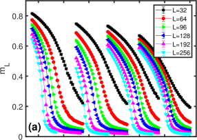
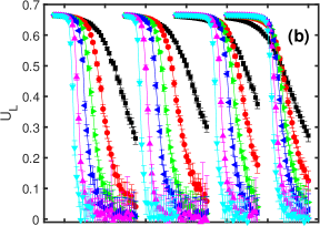
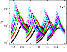
Figure 3: (a) Magnetization $m_{L}$, (b) reduced cumulant $U_{L}$, and (c) susceptibility $\chi_{L}$ plotted vs temperature $T$ for various different network sizes $L$, as indicated in panel (a). From right to left for $\alpha=0.1$, $\alpha=0.2$, $\alpha=0.4$, and $\alpha=0.8$.

At low values of $\alpha$, we observed that the system could not remain ordered in the thermodynamic limit, except for $\alpha=0$ , where we obtained the mean-field critical behavior from the model with long-range interactions independent of the distance between connected sites. This crossover behavior, where we can reach critical temperatures as low as the network size increases, is easily identified with the curves of thermodynamic quantities for different network sizes. These curves for different network sizes and low values of $\alpha$ can be seen in Fig. 3. In Fig. 3(a), the curves of $\textrm{m}_{\textrm{L}}$ can be seen showing the finite-size behavior, where the larger the network size and the smaller the value of $\alpha$, the faster the curves decay towards the disordered paramagnetic phase $P$. The same can be observed in Figs. 3(b) and (c) for the curves of $\textrm{U}_{\textrm{L}}$ and $\textrm{$\chi$}_{\textrm{L}}$, respectively.

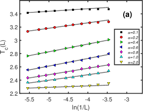
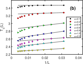
Figure 4: Pseudocritical temperature $T_{c}(L)$ as a function of (a) $\ln(1/L)$ and (b) $1/L$ for different values $\alpha$, as indicated in the figures.

To confirm the absence of a finite phase transition temperature for low values of $\alpha$, we can use the finite-size scaling behavior of $T_{c}(L)$ to extrapolates quite accurately the exact value in the thermodynamic limit $L\to\infty$. We used the peak of $\chi_{L}$ for different network sizes $L$, as it indicates the pseudo-critical temperature $T_{c}(L)$ of the system with linear size $L$. Therefore, we plotted $T_{c}(L)$ as a function of the inverse network size $1/L$. Consequently, the linear coefficient of the linear fit of the points gives us an estimate for the critical temperature $T_{c}\left(L\to\infty\right)$ in the thermodynamic limit. This is valid if there is a finite phase transition temperature, as we have the following scaling relation for finite systems, $T_{c}\left(L\right)=T_{c}\left(L\to\infty\right)\left(1-L^{-1/\nu}\right)$ [18]. In cases where the critical temperature does not have a linear behavior with the network size, that scaling relation is not valid, as is our case for low values of $\alpha<2$, as can be seen in Fig. 4.

Table 1: Values of the coefficients in the linear fit $T_{c}(L)=a+b\ln L$ based on the susceptibility peak, for some values of $\alpha$ in the crossover regime of the model.

$\alpha$			$a$			$b$
$0.1$			$3.6288\pm 0.0017$			$0.0381\pm 0.0073$
$0.2$			$3.5886\pm 0.0019$			$0.0812\pm 0.0094$
$0.4$			$3.4072\pm 0.0023$			$0.1159\pm 0.0176$
$0.6$			$3.1841\pm 0.0040$			$0.1144\pm 0.0243$
$0.8$			$2.9666\pm 0.0052$			$0.0969\pm 0.0238$
$1.0$			$2.8124\pm 0.0059$			$0.0827\pm 0.0251$

In Fig. 4(a), we can see that the curves with $\alpha\leq 1$ better fit the horizontal axis on the logarithmic scale, indicating a relationship between $T_{c}$ and the network size of the form $T_{c}\left(L\right)=a+b\ln L$. It is also noticeable that, similar to the case of the one-dimensional Ising model on an A-SWN network [14], the smaller the value of $\alpha$ the larger the network size needed to observe the correct behavior of $T_{c}$ as a function of $L$. Here, the logarithmic behavior was verified even for $\alpha=0.02$ with network size $L=768$, and we extended this result to smaller values of $\alpha$, having a finite phase transition temperature and mean-field critical behavior only at $\alpha=0$ [12, 13]. The values of the coefficients of the curves in Fig. 4(a) that exhibit logarithmic behavior can be found in Tab. 1.

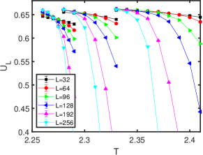
Figure 5: Binder cumulante $U_{L}$ plotted vs temperature $T$ for various different network sizes $L$, as indicated in the figure. From right to left for $\alpha=1.0$, $\alpha=1.3$, and $\alpha=1.7$.

The same curves from Fig. 4(a) are exhibited on a plot with a linear horizontal axis (see Fig. 4(b)), highlighting the incompatibility of the scaling, which is only valid for small network sizes at low $\alpha$ values. However, for $\alpha=2$ , we have verified that all network sizes are compatible with the linear scaling relationship of $T_{c}$ as a function of $L$, indicating a finite critical phase transition temperature.

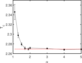
Figure 6: Critical temperature $T_{c}$ as a function of $\alpha$ near the transition point for the regime where the critical behavior of the system is described by the Ising model with short-range interactions. The red dotted line is a reference for the exact value $T_{c}$ of the 2D Ising model on a regular lattice.

Returning to an analysis of Fig. 3(b), we can observe a qualitative behavior indicating a transition between regimes. For $\alpha=0.1$, the Binder cumulant curves for different network sizes are closer to each other, even though there is no single crossing point. As $\alpha$ increases, these curves for different $L$ begin to diverge more significantly. Thus, for $\alpha=0$, there is a finite critical temperature, but for $\alpha\neq 0$, the system enters a crossover regime, which becomes increasingly pronounced as $\alpha$ increases, as shown by the slopes in Tab. 1. However, observing the slopes in Tab. 1, we can see that, they start to decrease above $\alpha=0.4$ suggesting the onset of a new finite temperature phase transition regime. This decreasing trend in the slopes continues up to around $\alpha=2$, as shown in Fig. 5. In this figure, we see that as $\alpha$ approaches $2$, the Binder cumulant curves get closer together, although they still do not exhibit a single crossing point.

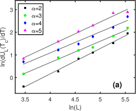
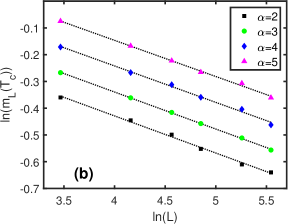
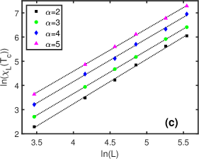
Figure 7: Log-log plot of (a) $m_{L}$, (b) $U_{L}$, and (c) $\chi_{L}$ near the critical point as a function of $L$, yielding the critical exponent ratios. In (a) the slope gives $1/\nu$, (b) $-\beta/\nu$, and (c) $\gamma/\nu$. The curves for different values of $\alpha$ as presented in the figures. The linear coefficients of the curves were adjusted for better visualization, and the error bars are smaller than the size of the symbols. The exponent ratios can be found in Tab. 2.

Table 2: Table of critical exponent ratios obtained from the linear fit of thermodynamic quantities at the critical point for some values of $\alpha$ in the short-range interaction regime of the model. The $T_{c}(L\rightarrow\infty)$ was estimated by extrapolation of the susceptibility peaks.

$\alpha$		$-\beta/\nu$		$\gamma/\nu$		$1/\nu$		$T_{c}(L\rightarrow\infty)$
$2$		$0.139\pm 0.01$		$1.84\pm 0.11$		$1.12\pm 0.12$		$2.271\pm 0.0020$
$3$		$0.138\pm 0.01$		$1.79\pm 0.04$		$0.94\pm 0.10$		$2.270\pm 0.0013$
$4$		$0.136\pm 0.02$		$1.78\pm 0.13$		$0.93\pm 0.13$		$2.268\pm 0.0015$
$5$		$0.135\pm 0.01$		$1.76\pm 0.06$		$1.03\pm 0.11$		$2.269\pm 0.0013$

The entry point into the new finite temperature phase transition regime was further identified by fitting $T_{c}$ as a linear function of $L^{-1}$. For this, we selected the value of $\alpha$ where we had an estimate of $T_{c}$ with an error less than $1\%$. This occurs near $\alpha=2$, and the behavior of $T_{c}$ as a function of $\alpha$ can be seen in Fig. 6. In this case, we observe that for values above $\alpha=2$, there are no significant changes in the critical temperature, and it is consistent with that obtained for the Ising model in two dimensions on a regular lattice, $T_{c}=2/\ln\left(1+\sqrt{2}\right)$[19]. The estimates of $T_{c}$ for $\alpha\geq 2$ presented in Fig. 6 can be found in Tab. 2.

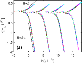
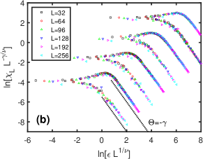
Figure 8: Data collapse into universal scaling functions (a) $m_{L}$ and (b) $\chi_{L}$ for different network sizes $L$, as displayed in panel (b). (a) From left to right, the collapse is plotted for $\alpha=2$, $\alpha=3$, $\alpha=4$, and $\alpha=5$, with the curves shifted horizontally by $5(\alpha-2)$ for better visualization. (b) From bottom to top, the collapse is plotted for $\alpha=2$, $\alpha=3$, $\alpha=4$, e $\alpha=5$, with the curves shifted by $2(\alpha-2)$ both vertically and horizontally for better visualization. For all these collapses were used $\beta=0.125$, $\gamma=1.75$, $\nu=1.0$, and the exact value $T_{c}$ of the Ising model on a regular 2D lattice. The dotted lines indicate the asymptotic behavior of the curves with slope $\Theta$.

In order to characterize the finite temperature regime for $\alpha\geq 2$ and to determine if, as predicted, it corresponds to the regime of the Ising model with short-range interactions, we must calculate the critical exponents of the system. The critical exponents were obtained using the scaling relations in Eqs 6, 7, and 8. By employing these relations, we can derive the exponents from the values of the relevant thermodynamic quantities near the critical point. This is achieved by log-log plot of these quantities as a function of the linear size of the network. The slope of the linear fit to the data points then yields the critical exponent ratios.

Fig. 7(a) displays the value of the derivative of the Binder cumulant near the critical point as a function of the linear size of the network on a log-log plot. Based on the scaling relation in Eq. 8, the slope of the linear fit to the points provides an estimate for the ratio $1/\nu$, which includes the exponent related to the system’s correlation length. Similarly, in Fig. 7(b), with the value of the magnetization near the critical point, the linear fit to the points, based on the scaling relation in Eq. 6, yields an estimate for the ratio $-\beta/\nu$, which includes the exponent related to the system’s order parameter. In Fig. 7(c), the magnetic susceptibility at the critical point, using the scaling relation in Eq. 7, allows us to estimate the ratio $\gamma/\nu$. These estimates can be found in Tab. 2, and, with the appropriate errors, they align with the critical exponents of the Ising model on a regular square lattice, which are $\beta=1/8$, $\gamma=7/4$ and $\nu=1$, confirmed both analytically and through Monte Carlo simulations [20].

The universal behavior for each scaling function, where different system sizes all collapse in one line, indicates that the critical exponents obtained for the system present reasonable precision. Therefore, another method to find the critical exponents of the system, though it will be used primarily here to verify the validity of the Ising model exponents in our system, is through data collapse. This method is also based on the scaling relations Eqs. 6, 7, and 8, and allows us to identify the form of the scaling function contained in these relations. If the correct critical exponents are applied to these scaling relations, for curves of different network sizes, we obtain a single curve that represents the scaling function of the system. Thus, verify if the critical exponents of the Ising model on a regular square lattice are applicable to our system, we have plotted $\textrm{m}_{\textrm{L}}L^{\beta/\nu}$ and $\textrm{$\chi$}_{\textrm{L}}L^{-\gamma/\nu}$ as a function of $L^{1/\nu}\epsilon$, with the exponents $\beta=1/8$, $\gamma=7/4$, and $\nu=1$. As a result, we obtained a single curve, which is the scaling function of the respective thermodynamic quantity.

The data collapse for $\textrm{m}_{\textrm{L}}$ and $\textrm{$\chi$}_{\textrm{L}}$ can be found in Fig. 8, showing that the system exhibits the behavior of the Ising model with short-range interactions, as a single curve is obtained for each value of $\alpha$ across different values of $L$. These plots use logarithmic scaling on the axes to provide additional confirmation of the exponents of the system through the asymptotic behavior of the curves away from $\epsilon=0$. The slope $\Theta=\beta$ is expected for $\epsilon<0$ and $\Theta=\beta-\nu$ for $\epsilon>0$ in the higher-order terms of $m_{0}$ from Eq. 6, and $\Theta=-\gamma$ in the higher-order terms of $\chi_{0}$ from Eq. 7.

IV Conclusions

In this work, we studied the Ising model on a 2D A-SWN, where the long-range interactions $J_{ij}$ depend on the geometric distance $r_{ij}$ between connected sites $i$ and $j$, such as $J_{ij}=r_{ij}^{-\alpha}$. We found that the mean-field critical behavior is achieved only at $\alpha=0$. For $\alpha>0$ , the system enters a crossover regime where no magnetic ordering is observed in the thermodynamic limit $L\rightarrow\infty$, as critical temperatures decrease with increasing network size. However, for $\alpha\geq 2$, the system maintains magnetic ordering due to the diminished influence of long-range interactions, reaching the regime where the critical behavior is governed by the short-range interaction Ising model. Compared to the globally coupled model, which has $N(N-1)/2$ edges, does not exhibit the crossover behavior observed in the A-SWN, in both one and two dimensions, and achieves mean-field critical behavior at $\alpha\neq 0$. This difference can be attributed to the limited number of long-range interactions in the A-SWN, with only $N$ edges. Analyzing $J_{ij}$ as a function of $\alpha$ in Fig. 2, we observed that for $0<\alpha<2$, the different network sizes show different decay rates of long-range interaction strength. This, combined with the limited number of interactions, may also explain the emergence of the crossover regime in the system. However, further studies are required to verify this assertion, where $J_{ij}$ as a function of $\alpha$ should exhibit the same behavior for any network size.

References

- [1] S. Mingram, Psychol. Today 2, 60 (1967).
- [2] D. J. Watts, and S.H. Strogatz, Nature 393, 440 (1998).
- [3] M. E. J. Newman, and D. J. Watts, Phys. Rev. E 60, 7332 (1999).
- [4] E. Ising, Z. Physik 31, 253 (1925).
- [5] M.E. Fisher, S.-k. Ma, and B.G. Nickel, Phys. Rev. Lett. 29, 917 (1972).
- [6] T. Blanchard, M. Picco, and M. A. Rajabpour, EPL 101, 56003 (2013).
- 7 [20] A. L. M. Vilela, B. J. Zubillaga, C. Wang, M. Wang, R. Du, and H. E. Stanley, Scy. Rep. 10, 8255 (2020).
- 8 [20] B. J. Zubillaga, A. L. M. Vilela, M. Wang, R. Du, G. Dong, and H. E. Stanley, Scy. Rep. 12, 282 (2022).
- 9 [20] D. S. M. Alencar, T. F. A. Alves, R. S. Ferreira, F. W. S. Lima, G. A. Alves, and A. Marcelo-Filho, Physica A, 626, 129102 (2023).
- 10 [20] J. Wang, Wei Liu, F. Wang, Z. Li and K. Xiong, Eur. Phys. J. B, 22, 97 (2024).
- 11 [20] H. Hong, Beom Jun Kim, and M. Y. Choi, Phys. Rev. E 66, 018101 (2002).
- 12 [20] C. P. Herrero, Phys. Rev. E 65, 066110 (2002).
- 13 [20] R. A. Dumer, and M. Godoy, Eur. Phys. J. B 95, 159 (2022).
- 14 [20] D. Jeong, H. Hong, B. J. Kim, and M. Y. Choi, Phys. Rev. E 68, 027101 (2003).
- 15 [20] N. Metropolis, A. W. Rosenbluth, M. N. Rosenbluth, and A. H. Teller, J. Chem. Phys. 21, 1087 (1953).
- 16 [20] M. E. J. Newman and G. T. Barkema. Monte Carlo Methods in Statistical Physics, 1st ed. (Oxford University Press, NewYork, EUA, 1999).
- 17 [20] L. B ttcher and H. J. Herrmann. Computational Statistical Physics, 1st ed. (Cambridge University Press, NewYork, EUA, 2021).
- 18 [20] R. T. Scalettar, Physica A, 170, 282 (1991).
- 19 [20] L. Onsager, Phys. Rev. 65, 117 (1944).
- 20 [20] G. dor, Rev. Mod. Phys. 76, 663 (2004).