Joint Approximate Partial Diagonalization of Large Matrices

Abstract

Given a set of $p$ symmetric (real) matrices, the Orthogonal Joint Diagonalization (OJD) problem consists of finding an orthonormal basis in which the representation of each of these $p$ matrices is as close as possible to a diagonal matrix. We argue that when the matrices are of large dimension, then the natural generalization of this problem is to seek an orthonormal basis of a certain subspace that is a near eigenspace for all the matrices in the set. We refer to this as the problem of “partial joint diagonalization of matrices.” The approach proposed first finds this approximate common near eigenspace and then proceeds to a joint diagonalization of the restrictions of the input matrices in this subspace. A few solution methods for this problem are proposed and illustrations of its potential applications are provided.

Keywords: orthogonal joint diagonalization, blind source separation, independent component analysis, invariant subspaces, partial diagonalization, FMRI.

AMS: 15A69, 15A18

1 Introduction and problem statement

Given $p$ symmetric positive definite matrices $C_{1},C_{2},\cdots,C_{p}$, each of size $n\times n$ the standard Orthogonal Joint Diagonalization (OJD) problem consists of finding a common $n\times n$ unitary matrix $Q$ such that each $Q^{T}C_{i}Q$ is as close as possible to a diagonal $D_{i}$. Note at the outset that in the ‘exact’ case when there is a matrix $Q$ such that $C_{i}=QD_{i}Q^{T}$ for $i=1,\cdots,p$, then the columns of $Q$ are the eigenvectors of any one of the matrices, so in theory the solution is completely determined by any one matrix in the set. Issues of uniqueness have been studied in [2]. Here, uniqueness is meant up to permutations and sign scalings of the columns of $Q$.

An important source of joint diagonalization problems is in Blind Source Separation (BSS) and independent component analysis (ICA). A typical example can be described as follows. Let $\textbf{s}(t)$ be an $M$-dimensional vector containing the time series of $M$ mutually independent source signals that are mixed by a mixing matrix $\textbf{A}^{n\times M}$, so that $\textbf{x}(t)=\textbf{A}\textbf{s}(t)$ is an $n$-dimensional vector containing the time series of $n$ mixture signals. In BSS one aims to recover the source signals $\textbf{s}(t)$ from the observed mixtures $\textbf{x}(t)$ without knowing A or the distribution of the sources but with the assumption that the sources signals are nonstationary and mutually independent. The set of matrices to joint diagonalize in this case can be obtained from covariance matrices estimated on different time windows or intercorrelation matrices with time shifts [3]. The diagonal matrices in this case correspond to covariance matrices or intercorrelation matrices of the source signals. These matrices are time varying but have always diagonal structures. Alternative approaches to construct the set of matrices to joint diagonalize can be obtained by using linear combinations of intercorrelation matrices [26], slices of higher order cumulants tensors [6], time-frequency matrices [9] or second derivatives of the log characteristic function [27].

The various algorithms that have been developed to solve this problem differ in the way in which the actual optimization problem is solved and what restrictions on the mixing matrix this implies. They can be classified into orthogonal joint diagonalization and non-orthogonal joint diagonalization (NOJD) methods. The most popular algorithm for the OJD problem is JADE [7], a Jacobi-like algorithm based on plane rotations. In BSS applications, the assumption of orthogonal mixing and demixing matrices can often be inappropriate. In such situations, methods that work with nonorthogonal matrices are preferred [28][25][21][1].

Most previous work in this area focused on the small (dense) case, see, e.g., [24, 5, 4, 10], among many others. In large applications where the signal vectors can consist of hundreds or more of variables, existing joint diagonalization algorithms cannot be applied due to their exorbitant computational cost or simply because they diverge for high dimensional data sets. The case of large matrices has important applications in which the $C_{i}$’s are often covariance matrices. Thus, the article [23] discusses ‘subspace coloring’ to tackle the autocorrelation structure They propose a dimension reduction method that evaluates the time structure of multivariate observations, see also [3]. Their goal is to differentiate the signal subspace from noise by extracting a subspace of non trivially autocorrelated data. In other words, their method is to find a common invariant subspace for a set of correlation matrices $R_{\tau}$ where the $\tau$’s correspond to a few time-lags.

The first question we address in this paper is to define a natural extension of the OJD for large dimensional cases. For this it is important to think in terms of subspaces. In this regard, the algorithms we propose are neither orthogonal or non-orthogonal but approximate orthogonal. Indeed, in practical high dimensional data application, the investigator is often interested only in a subset of variables that lie in a subspace of dimension $k\ll n$. The underlying assumption is that the selected subspace concentrates most of the information (variability) of the data set. The matrices are to be jointly diagonalized only in this subspace.

2 Approximate Joint Partial Diagonalization

A common formulation of the standard OJD is to seek an $n\times n$ orthogonal matrix $Q$ that minimizes

$$f_{0}(Q)=\sum_{i=1}^{p}\|\texttt{Off}(Q^{T}C_{i}Q)\|_{F}^{2},$$ (1)

where $\texttt{Off}(X)$ denotes the matrix $X$ with its diagonal entries replaced by zeros. In situations where the matrices are large, methods based on minimizing the above objective function over unitary matrices $Q$, become too expensive, their costs being of the order $O(pn^{3})$ where $n$ is the size of the matrices. Our first goal is to define a generalization of the problem that can cope with large, possibly sparse, matrices, while keeping the motivation and rationale of the small dense case.

2.1 Joint eigenspaces

The main change needed to generalize the joint diagonalization problem to large matrices is to require that the orthogonal matrix $Q$ be of size $n\times k$ where $k$ is small. In addition, we would also like $Q$ to represent the basis of a common nearly invariant subspace for all $C_{i}$’s. With this, it is clear that a straightforward extension of the formulation represented by (1) is not too meaningful. Consider a naive generalization of the problem the problem that would consist of simply finding an orthogonal matrix (i.e., a matrix with orthonormal columns) $Q\in\mathbb{R}^{n\times k}$ ($k$ columns) so as to minimize the same objective function (1). This clearly does not work in that it will not yield a basis of a subspace with the desired property of near invariance by all matrices $C_{i}$. For example, consider the following 3 matrices $C_{i},i=1,2,3$ (only lower parts are shown due to symmetry) and assume we take $k=2$.

$$\left[\begin{array}[]{cc|ccc}x&&&&\\ &x&&&\\ \hline\cr x&&x&&\\ &x&x&x&\\ x&&&x&x\end{array}\right]\quad\left[\begin{array}[]{cc|ccc}x&&&&\\ &x&&&\\ \hline\cr x&&x&&\\ x&x&&x&\\ &x&&x&x\end{array}\right]\quad\left[\begin{array}[]{cc|ccc}x&&&&\\ &x&&&\\ \hline\cr x&&x&&\\ &x&&x&\\ x&x&x&&x\end{array}\right]$$

In this example all $C_{i}$’s happen to have a $k\times k$ leading block $C_{i}(1:k,1:k)$ that is diagonal. Here, the optimal solution to the problem (1) is clearly the matrix $Q$ consisting of the first $k$ columns of the $n\times n$ identity matrix. If entries in the blocks (2,1) (and (1,2) by symmetry) were small in magnitude and if diagonal entries on the (1,1) block of each $C_{i}$ are near the largest eigenvalues of $C_{i}$, then this $Q$ would be a good solution because it would represents the basis of a subspace that is near the dominant invariant subspace for each of the 3 matrices. Otherwise, i.e., in the case where entries in the $(1,2)$ blocks are large, this optimal solution is not too meaningful.

Therefore, the primary problem we address in this paper is to find a matrix $Q$ that is of size $n\times k$, with orthonormal columns such that the span of $Q$ is nearly invariant by each $C_{i}$, i.e., such that $C_{i}Q\approx QD_{i}$ for some $k\times k$ matrix $D_{i}$. In addition, we would like this common invariant subspace to be ‘dominant’ for each $C_{i}$, i.e., associated with the largest eigenvalues for each $C_{i}$. Note that the requirement that each $D_{i}$ be diagonal, which was imposed in the standard case, is being omitted for now. Later, we will see that we can obtain the desired near-diagonal structure in a post-processing phase once the common invariant subspace has been identified.

One of several ways of formulating the problem rigorously, is to state that we seek an orthogonal matrix $Q\in\mathbb{R}^{n\times k}$ and $k\times k$ matrices $D_{i}$, for $i=1,\cdots,p$ that minimize the objective function

$$f(Q,D_{1},...,D_{p})=\sum_{i=1}^{p}\|C_{i}Q-QD_{i}\|_{F}^{2}.$$ (2)

Consider each of the terms in the sum (2). A simple version of Theorem 2.6 in [22] shows that once $Q$ is known, each $D_{i}$ is uniquely determined. Indeed, let $C\,\in\,\mathbb{R}^{n\times n}$,  $D\,\in\,\mathbb{R}^{p\times p}$ and $R=CQ-QD$ where $Q\in\,\mathbb{R}^{n\times p}$ is a (fixed) orthogonal matrix. Then the theorem states that in any unitarily invariant norm $\|R\|$ is minimized when $D=Q^{T}CQ$. The matrix $CQ-Q(Q^{T}CQ)$ is treated as a residual matrix when $Q$ is considered as an approximate eigenspace. This theorem will play a key role in the analysis and so we show a slightly more elaborate version in Section 3.

Since each of the norms $\|C_{i}Q-QD_{i}\|_{F}$ represents a sort of measure of the invariance of the span of $Q$ by $C_{i}$, minimizing (2) will produce a common near eigenspace for the $C_{i}$’s. In realistic applications, such a subspace does not exist, but there is a common subspace of small dimension $k$ that is ‘almost invariant’ by all $C_{i}$’s may arise naturally in some applications. This translates into the existence of a matrix $Q$ (orthogonal basis of this subspace) and matrices $D_{i}$, $i=1,\cdots,p$ such that each for the norms $\|C_{i}Q-QD_{i}\|$ is small.

2.2 Joint partial diagonalization

The requirement that the $D_{i}$’s be diagonal has been relaxed so far but we can make the $D_{i}$’s diagonal in a post-processing phase by a ‘rotation’ of the bases. In a trivial approach to the problem, we could just diagonalize each $D_{i}$ separately as $D_{i}=W_{i}\Lambda_{i}W_{i}^{T}$, where $W_{i}\in\mathbb{R}^{k\times k}$, $W_{i}^{T}W_{i}=I$, and $\Lambda_{i}$ is diagonal. Then

$$\|C_{i}Q-QD_{i}\|_{F}=\|C_{i}(QW_{i})-(QW_{i})\Lambda_{i}\|_{F}.$$ (3)

Thus, each $C_{i}$ has been partially diagonalized with orthogonal matrices of the form $QW_{i}$, where each $W_{i}$ is $k\times k$ and unitary. These orthogonal bases $QW_{i}$ span the same space which is a nearly invariant subspace for each $C_{i}$ as desired but each orthogonal basis $Q_{i}\equiv QW_{i}$ is different for each $C_{i}$’. This solution answers a slightly different question from the standard one.

It is possible to make all matrices $Q^{T}C_{i}Q$ nearly diagonal with the same matrix $Q$ as is done in the classical case, to obtain in this way an approximate common partial diagonalization. A first approach to the proble is to rely on orthogonal transformations. Let $D_{i}=Q^{T}C_{i}Q$ for $i=1,\cdots,p$ and assume that the $D_{i}$’s can be approximately jointly diagonalized. Then there exists a matrix $W\in\mathbb{R}^{k\times k}$, with $W^{T}W=I$, such that $D_{i}W\approx W\Lambda_{i}$ for $i=1,2,\cdots,p$, where $\Lambda_{i}$ is diagonal. If, in addition, $C_{i}Q\approx QD_{i}$, then

$$C_{i}QW\approx(QW)W^{T}D_{i}W\approx(QW)\Lambda_{i}.$$

This results in an approximate joint diagonalization of the $C_{i}$’s by the orthogonal matrix $QW$. We will later analyze the error made in this 2-step process and show that the square of the Frobenius norm of the error is just the sum of the square of the Frobenius norms of the errors made in the two steps.

A second approach, which can be termed non-orthogonal, is seek a partial diagonalization of the $C_{i}$’s by congruence transformations. From the first step, we obtain the approximation:

$$Q^{T}C_{i}Q\approx D_{i}.$$

Then in a second step, a common $k\times k$ congruence transformation is applied to the $D_{i}$’s so that $L^{T}D_{i}L\approx\Lambda_{i}$ and therefore:

$$L^{T}Q^{T}C_{i}QL\approx\Lambda_{i}.$$

Now we have a basis, namely $QL$, of a nearly invariant subspace in which each $C_{i}$ has a nearly diagonal representation. We will not consider non-orthogonal transformations in this paper but wish to emphasize here that it is also possible to partly diagonalize the $C_{i}$’s with non-orthogonal transformations.

2.3 General approach

The main method introduced in this paper solves the decoupled formulation of the problem as described above. In a first stage, the objective function (2) is minimized with respect to $Q$ and the $D_{i}$’s only, ignoring the diagonal structure requirement for the $D_{i}$’s. This yields an orthogonal matrix $Q$ and matrices $D_{i}$, so that $C_{i}Q\approx QD_{i}$, for $i=1,\cdots,p$, i.e., $Q$ represents the basis of a nearly invariant subspace common to all the $C_{i}$’s.

If desired, the resulting approximate factorizations $C_{i}Q\approx QD_{i}$, can be post-processed in a second stage to get a joint partial diagonalization of the $C_{i}$’s. This is done via the solution of a standard, orthogonal or non-orthogonal, joint diagonalization of the $D_{i}$’s as described in the previous subsection. This standard joint diagonalization problem involves the matrices $D_{i}$, which are of size $k\times k$ where $k$ is typically small.

3 General results

The objective function (2) is not convex with respect to $Q,\{D_{i}\}$ together. It is however quadratic with respect to $Q$ alone, and each $D_{i}$ alone. As it turns out we can optimize the objective by focussing on $Q$ alone. The $D_{i}$’s will be obtained immediately once the optimal $Q$ is known. This section discusses this and related issues.

Recall that when we consider matrices as vectors in $\mathbb{R}^{n^{2}}$, the usual Euclidean inner product translates into the Frobenius inner product of matrices

$$\left\langle A,B\right\rangle=\text{Trace}\ [B^{T}A].$$ (4)

In particular $\|X\|_{F}^{2}=\text{Trace}[X^{T}X]$. In addition, we will say that $A\perp_{F}B$ if $\left\langle A,B\right\rangle=0$. If $Q$ is an $n\times k$ orthogonal matrix then the orthogonal projector onto the span of $Q$, which we will call $P$, is represented by the matrix $P=QQ^{T}$. Hidden in this notation is the fact that the same $P$ is represented in this form for different orthogonal bases of the same subspace.

3.1 Problem decoupling

The first question we address is: Assuming that $Q$ is fixed, what is the best set of $D_{i}$’s that minimize (2)? Note that the resulting optimization problem decouples into $p$ subproblems. Indeed, in order to minimize

$$\sum_{i=1}^{p}\|C_{i}Q-QD_{i}\|_{F}^{2}$$

with respect to the $D_{i}$’s, we can minimize each of the terms separately. The following result is a reformulation of Theorem 2.6 in [22].

Theorem 1.

For a fixed orthogonal matrix $Q$, define $D_{Q,i}=Q^{T}C_{i}Q$. Then the objective function (2) is minimized when $D_{i}=D_{Q,i}$. In addition, if we define the residual matrix as $R_{i}=C_{i}Q-QD_{Q,i}$ then $R_{i}=(I-QQ^{T})C_{i}Q$ and in particular $R_{i}\perp_{F}Q$ and $\|R_{i}\|_{F}=\|(I-QQ^{T})C_{i}Q\|_{F}$.

Proof.

We start with the following relation:

$$C_{i}Q-QD_{i} = QQ^{T}C_{i}Q+(I-QQ^{T})C_{i}Q-QD_{i}$$

$$= Q(Q^{T}C_{i}Q-D_{i})+(I-QQ^{T})C_{i}Q.$$

Exploiting the orthogonality of matrices of the form $QX$ and $(I-QQ^{T})Y$ we obtain:

$$\|C_{i}Q-QD_{i}\|_{F}^{2}=\|Q(Q^{T}C_{i}Q-D_{i})\|_{F}^{2}+\|(I-QQ^{T})C_{i}Q\|_{F}^{2}$$

which shows that the minimum is indeed achieved for $D_{i}=Q^{T}C_{i}Q$. In this case $R_{i}=(I-QQ^{T})C_{i}Q$. As a result it is clear that $R_{i}\perp_{F}Q$ and that the error term relative to $C_{i}$ is $\|R_{i}\|_{F}=\|(I-QQ^{T})C_{i}Q\|_{F}.$ This completes the proof. ∎

We emphasize an important result of the theorem which is that the residual $R_{i}$ is orthogonal to $Q$ in the Frobenius inner product sense, i.e., $\text{Trace}(Q^{T}R_{i})=0$. However, it is clear that the stronger result $Q^{T}R_{i}=0$ is also true.

As mentioned in the introduction, we can first optimize (2) with respect to $Q$ only and then find an optimal joint diagonalization for the $D_{i}$. Both steps incur an error and it turns out that these two errors decouple.

Proposition 2 (Error decoupling).

Assume that we find a joint orthogonal matrix $Q$ such that

$$C_{i}Q-QD_{i}=E_{i}\quad i=1,\cdots,p$$ (5)

where $D_{i}=Q_{i}^{T}C_{i}Q_{i}$, and that an approximate joint diagonalization of the matrices $D_{i}$’s is available with:

$$D_{i}W-W\Lambda_{i}=F_{i},\ \quad i=1,\cdots,p.$$ (6)

Define $\tilde{Q}=QW$. Then,

$$\sum_{k=1}^{p}\|C_{i}\tilde{Q}-\tilde{Q}\Lambda_{i}\|_{F}^{2}=\sum_{k=1}^{p}\left[\|E_{i}\|_{F}^{2}+\|F_{i}\|_{F}^{2}\right].$$ (7)

Proof.

For each $i$: $C_{i}\tilde{Q}-\tilde{Q}\Lambda_{i}=C_{i}QW-QW\Lambda_{i}=C_{i}QW-Q(D_{i}W-F_{i})$. Hence

$$\sum_{i=1}^{p}\|C_{i}\tilde{Q}-\tilde{Q}\Lambda_{i}\|_{F}^{2} = \sum_{i=1}^{p}\|(C_{i}QW-QD_{i}W)+QF_{i}\|_{F}^{2}$$

$$= \sum_{i=1}^{p}\|[(C_{i}Q-QD_{i})+QF_{i}W^{T}]W\|_{F}^{2}$$

$$= \sum_{i=1}^{p}\|E_{i}+QF_{i}W^{T}\|_{F}^{2}\ .$$

Since each $E_{i}=C_{i}Q-QD_{i}$ is orthogonal to $Q$ in the sense of the Frobenius inner product we have:

$$\sum_{i=1}^{p}\|E_{i}+QF_{i}W^{T}\|_{F}^{2} = \sum_{i=1}^{p}\|E_{i}\|_{F}^{2}+\|QF_{i}W^{T}\|_{F}^{2}$$

$$= \sum_{i=1}^{p}\|E_{i}\|_{F}^{2}+\|F_{i}\|_{F}^{2}.$$

∎

If the errors decouple, can we say that the two optimization problems decouple as well? As it turns out the matrices $\Lambda_{i}$ for the second optimization problem (JOD of the $D_{i}$’s) are also determined from the knowledge of the optimal $Q$.

Theorem 3.

Let ${\underline{Q}}$ an $n\times k$ orthogonal matrix and ${\underline{\Lambda}}_{i}$, $i=1,\cdots,p$ diagonal matrices such that $f({\underline{Q}},{\underline{\Lambda}}_{1},\cdots,{\underline{\Lambda}}_{p})$ is minimum. Then ${\underline{\Lambda}}_{i}=\mathop{\operator@font diag}\nolimits({\underline{Q}}^{T}C_{i}{\underline{Q}})$ for $i=1,\cdots,p$. In addition, for this ${\underline{Q}}$ the objective function (2) is equal to:

$$f({\underline{Q}},{\underline{\Lambda}}_{1},\cdots,{\underline{\Lambda}}_{p})=g({\underline{Q}})\equiv\sum_{i=1}^{p}\left[\|C_{i}{\underline{Q}}-{\underline{Q}}D_{{\underline{Q}},i}\|_{F}^{2}+\|\texttt{Off}(D_{{\underline{Q}},i})\|_{F}^{2}\right],$$ (8)

where $D_{{\underline{Q}},i}={\underline{Q}}^{T}C_{i}{\underline{Q}}$.

Proof.

Consider one term in the sum (2) where ${\underline{Q}}$ is optimal. Dropping the index $i$ we denote by $D_{{\underline{Q}}}$ the matrix ${\underline{Q}}^{T}C{\underline{Q}}$ and recall that ${\underline{Q}}^{T}(C{\underline{Q}}-{\underline{Q}}D_{\underline{Q}})=0$. Then,

$$\|C{\underline{Q}}-{\underline{Q}}{\underline{\Lambda}}\|_{F}^{2} = \|C{\underline{Q}}-{\underline{Q}}D_{{\underline{Q}}}+{\underline{Q}}(D_{{\underline{Q}}}-{\underline{\Lambda}})\|_{F}^{2}$$

$$= \|C{\underline{Q}}-{\underline{Q}}D_{{\underline{Q}}}\|_{F}^{2}+\|{\underline{Q}}(D_{{\underline{Q}}}-{\underline{\Lambda}})\|_{F}^{2}$$

$$= \|C{\underline{Q}}-{\underline{Q}}D_{{\underline{Q}}}\|_{F}^{2}+\|D_{{\underline{Q}}}-{\underline{\Lambda}}\|_{F}^{2}.$$

The term $\|D_{{\underline{Q}}}-{\underline{\Lambda}}\|_{F}^{2}$ is smallest when ${\underline{\Lambda}}=\mathop{\operator@font diag}\nolimits(D_{{\underline{Q}}})$. This shows the first part. The second part follows by observing that for the optimal ${\underline{\Lambda}}$ we have $\|D_{{\underline{Q}}}-{\underline{\Lambda}}\|_{F}^{2}=\|\texttt{Off}(D_{{\underline{Q}}})\|_{F}^{2}$. ∎

The theorem shows that the problem of minimizing $f(Q,\Lambda_{1},\cdots,\Lambda_{p})$ where the $\Lambda_{i}$’s are diagonal, can be restated entirely in terms of the unknown matrix $Q$: it suffices to find an orthogonal $Q$ so that (8) is minimum. Each $\Lambda_{i}$ is then equal to $\texttt{Diag}(D_{Q,i})$.

The objective function $g$ defined in (8) can be split in two parts:

$$\gamma(Q)=\sum_{i=1}^{p}\|C_{i}Q-QD_{Q,i}\|_{F}^{2};\qquad\omega(Q)=\sum_{i=1}^{p}\|\texttt{Off}(D_{Q,i})\|_{F}^{2}.$$ (9)

Now we can think of a 2-stage, or decoupled, procedure. The first stage of this procedure finds an optimal $Q$ that minimizes $\gamma(Q)$. The second stage seeks a basis change $Q_{new}=QW$, where the desired $W\in\mathbb{R}^{p\times p}$ is unitary, and is selected so as to minimize $\omega(Q_{new})$. As the following Lemma shows, this second stage does not change the minimal value of $\gamma$ obtained in the first stage.

Lemma 4.

Let $W$ be any $k\times k$ unitary matrix and let $\gamma(Q)$ defined in (9). Then

$$\gamma(Q)=\gamma(QW).$$ (10)

Proof.

We have

$$\|C_{i}Q-QD_{Q,i}\|_{F}^{2} = \|C_{i}QW-QD_{Q,i}W\|_{F}^{2}$$

$$= \|C_{i}(QW)-(QW)W^{T}D_{Q,i}W\|_{F}^{2}$$

$$= \|C_{i}(QW)-(QW)[(QW)^{T}C_{i}(QW)]\|_{F}^{2}.$$

This completes the proof by noting that $(QW)^{T}C_{i}(QW)\equiv D_{QW,i}$. ∎

The lemma establishes that $\gamma(Q)$ is a function of the subspace only, not its basis $Q$.

Consider now a certain $\tilde{Q}$ found in a first stage to minimize $\gamma(Q)$. In the second stage we wish to minimize $\omega(Q)$ over different orthonormal bases $Q=\tilde{Q}W$ of the same subspace. Note that for any unitary $W$, we have

$$D_{QW,i}=(QW)^{T}C_{i}(QW)=W^{T}D_{Q,i}W.$$

As a result, the best $W$ can be found by jointly minimizing the second term of the objective function, namely:

$$\sum_{i=1}^{p}\|\texttt{Off}[W^{T}D_{\tilde{Q},i}W]\|_{F}^{2},$$ (11)

over $W$. This is the classical joint diagonalization problem but it now involves small matrices of size $k\times k$.

Proposition 5.

A minimizer $Q_{*}$ of the objective function (8) is of the form $Q_{*}=\tilde{Q}W$ where $\tilde{Q}$ minimizes the function $\gamma(Q)$ over all orthogonal $m\times p$ matrices, and $W$, minimizes (11), i.e., it solves a standard orthogonal joint diagonalization problem for the matrices $D_{\tilde{Q},i}=\tilde{Q}^{T}C_{i}\tilde{Q}_{i}$, $i=1,\cdots,p$.

Proof.

The proof follows from the lemma and the discussion above. ∎

The 2-stage procedure just described is sketched below as Algorithm 1.

Algorithm 1 Decoupling procedure

1:Find an orthogonal $Q$ that minimizes $\gamma(Q)=\sum_{i=1}^{p}\|C_{i}Q-QD_{Q,i}\|_{F}^{2}$

2:Find a unitary matrix $W\ \in\mathbb{R}^{k\times k}$ that minimizes (11)

3:Output $\tilde{Q}\equiv QW$ and $\tilde{\Lambda}_{i}=\mathop{\operator@font diag}\nolimits[\tilde{Q}^{T}C_{i}\tilde{Q}]=\mathop{\operator@font diag}\nolimits[W^{T}D_{Q,i}W]$

Observe that the algorithm will yield an orthogonal matrix $\tilde{Q}$ and diagonal matrices $\tilde{\Lambda}_{1},\cdots,\tilde{\Lambda}_{p}$ such that $\gamma(\tilde{Q})=\gamma(QW)$ is minimum over orthogonal matrices $Q$ and, exploiting orthogonality as in the proof of Theorem 3 we get

$$\sum_{i=1}^{p}\|C_{i}\tilde{Q}-\tilde{Q}\tilde{\Lambda}_{i}\|_{F}^{2} = \sum_{i=1}^{p}\|[C_{i}\tilde{Q}-\tilde{Q}D_{\tilde{Q}_{i}}]+\tilde{Q}[D_{\tilde{Q}_{i}}-\tilde{\Lambda}_{i}]\|_{F}^{2}$$

$$= \sum_{i=1}^{p}\|C_{i}\tilde{Q}-\tilde{Q}D_{\tilde{Q}_{i}}\|_{F}^{2}+\sum_{i=1}^{p}\|\tilde{Q}[D_{\tilde{Q}_{i}}-\tilde{\Lambda}_{i}]\|_{F}^{2}$$

$$= \gamma(\tilde{Q})+\sum_{i=1}^{p}\|D_{\tilde{Q}_{i}}-\tilde{\Lambda}_{i}\|_{F}^{2}=\gamma(\tilde{Q})+\sum_{i=1}^{p}\|\texttt{Off}[D_{\tilde{Q}_{i}}]\|_{F}^{2}$$

The last equality comes from the definition of $\tilde{\Lambda}_{i}$. This establishes the relation

$$f(\tilde{Q},\{\tilde{\Lambda}_{i}\}_{i=1:p})=\sum_{i=1}^{p}\|C_{i}\tilde{Q}-\tilde{Q}\tilde{\Lambda}_{i}\|_{F}^{2}=\gamma(\tilde{Q})+\omega(\tilde{Q})$$ (12)

which shows a similar result to that of Theorem 3 for $\tilde{Q}$.

We may now ask whether or not the above procedure can recover a solution that is the same or close to the optimal one for (2) in which the additional constraint that each $D_{i}$ be diagonal is enforced. Let $\tilde{Q}$ be the matrix that results from the decoupling procedure of Algorithm 1. At the same time let ${\underline{Q}},{\underline{\Lambda}}_{1},\cdots,{\underline{\Lambda}}_{p}$ be a minimizing set of matrices for (2) as defined in Theorem 3. Then because $\tilde{Q}$ minimizes $\gamma$ we clearly have

$$\gamma(\tilde{Q})\leq\gamma({\underline{Q}})\ .$$ (13)

Now, from Theorem 3, the optimal value of the objective function is equal to:

$$f({\underline{Q}},{\underline{\Lambda}}_{1},\cdots,{\underline{\Lambda}}_{p})=\gamma({\underline{Q}})+\omega({\underline{Q}})$$ (14)

On the other hand, the set $\tilde{Q},\{\tilde{\Lambda}_{i}\}_{i=1:p}$ realizes a partial orthogonal diagonalization and so:

$$f({\underline{Q}},{\underline{\Lambda}}_{1},\cdots,{\underline{\Lambda}}_{p})\leq f(\tilde{Q},\tilde{\Lambda}_{1},\cdots,\tilde{\Lambda}_{p})$$ (15)

Putting the above relations together will give the following corollary.

Corollary 6.

With the notation of Theorem 3 and Algorithm 1, the following double inequality is satisfied:

$$f(\tilde{Q},\{\tilde{\Lambda}_{i}\}_{i=1:p})-[\omega(\tilde{Q})-\omega({\underline{Q}})]\leq f({\underline{Q}},\{{\underline{\Lambda}}_{i}\}_{i=1:p})\leq f(\tilde{Q},\{\tilde{\Lambda}_{i}\}_{i=1:p})\ .$$ (16)

Proof.

The right part of (16) is just (15). From (14) and (13) we get

$$f({\underline{Q}},{\underline{\Lambda}}_{1},\cdots,{\underline{\Lambda}}_{p})=\gamma({\underline{Q}})+\omega({\underline{Q}})\geq\gamma(\tilde{Q})+\omega({\underline{Q}}).$$

This yields the first inequality after substituting the value of $\gamma(\tilde{Q})$ extracted from equality (12). ∎

A by-product of the result is that the difference $\omega(\tilde{Q})-\omega({\underline{Q}})$ is nonnegative. It is zero when the optimal solution is also the optimal solution obtained by the decoupling algorithm. This happens when there exists an exact joint diagonalization of the projected set $\{D_{\tilde{Q},i}\}_{i=1,\cdots,p}$. In this situation, $\omega(\tilde{Q})=0$ which forces $\omega({\underline{Q}})$ to also equal zero since $\omega(\tilde{Q})\geq\omega({\underline{Q}})$ and then (16) implies that $f({\underline{Q}},\{{\underline{\Lambda}}_{i}\}_{i=1:p})=f(\tilde{Q},\{\tilde{\Lambda}_{i}\}_{i=1:p})$. In case the matrices $D_{\tilde{Q},i}$ can be jointly diagonalized only inexactly, then the optimal objective functions obtained by the exact optimum and the decoupled one differ by $\omega(\tilde{Q})-\omega({\underline{Q}})$. This difference will be small if $\omega(\tilde{Q})$ is small, i.e., if the set $\{D_{\tilde{Q},i}\}$ is nearly jointly diagonalizable.

As a final note, we should mention that no statement was made on the closeness of the subspace obtained by the decoupling procedure to the optimal one. The lack of uniqueness implies that even if the related objective functions are equal, we cannot say that the subspaces are the same or close.

3.2 The Grassmannian perspective

As already stated, Algorithm 1 in the simple form given above does not specify which of the many possible nearly invariant subspaces is selected when minimizing $\gamma(Q)$. In typical applications, it is the subspace associated with the largest $p$ eigenvalues for each $C_{i}$ that is desired. We could consider instead the objective function:

$$\phi(Y)=\frac{1}{2}\sum_{i=1}^{p}\text{Trace}[Y^{T}C_{i}Y].$$ (17)

We changed notation from $Q$ to $Y$ to reflect a more generally adopted notation in this context. In the case when $p=1$, it is well-known [12, 10.6.5] that maximizing the above trace over orthogonal matrices $Y$ will yield an orthogonal basis for the invariant subspace associated with the largest $p$ eigenvalues. This is exploited in the TraceMin algorithm [18, 19] a method designed for computing an invariant subspace associated with smallest eigenvalues for standard and generalized eigenvalue problems.

Unfortunately when $p>1$ the optimum is just the dominant subspace of the matrix $\sum_{i=1}^{p}C_{i}$. Indeed, maximizing (17) is oblivious to the invariance of $[Y]$ with respect to each matrix $C_{i}$. This is just the opposite of what is obtained when minimiming $\gamma(Y)$: optimize invariance regardless of which subspace is obtained. What is needed is a criterion that mixes the two objective functions. An objective function similar to (17) was also proposed in [23] where the trace in (17) is replaced by the Frobenius norm squared:

$$\psi(Y)=\frac{1}{2}\ \sum_{i=1}^{p}\|Y^{T}C_{i}Y\|_{F}^{2}.$$

Let us examine this alternative. First note that due to symmetry, $\|Y^{T}C_{i}Y\|_{F}^{2}=\frac{1}{2}\text{Trace}[Y^{T}C_{i}YY^{T}C_{i}Y]$. Then letting $\Pi=YY^{T}$, we have:

$$\text{Trace}(Y^{T}C_{i}\Pi C_{i}Y) =\text{Trace}(Y^{T}C_{i}(I-(I-\Pi))C_{i}Y)$$

$$=\text{Trace}(Y^{T}C_{i}^{2}Y)-\text{Trace}(Y^{T}C_{i}(I-\Pi)C_{i}Y)$$

$$=\text{Trace}(Y^{T}C_{i}^{2}Y)-\text{Trace}(Y^{T}C_{i}(I-\Pi)(I-\Pi)C_{i}Y)$$

$$=\text{Trace}(Y^{T}C_{i}^{2}Y)-\|(I-\Pi)C_{i}Y\|_{F}^{2}$$

and upon summation we therefore get:

$$\psi(Y)=\frac{1}{2}\sum_{i=1}^{p}\text{Trace}(Y^{T}C_{i}^{2}Y)-\frac{1}{2}\gamma(Y).$$ (18)

Thus, this alternative provides the desired mixing of the objective functions: by maximizing $\psi(Y)$ we maximize the sum of the traces of $Y^{T}C_{i}^{2}Y$ while at the same time making the invariance mesure $\gamma(Y)$ small as desired. Note that we could also replace the matrices $C_{i}^{2}$ in the first term by $C_{i}$ as an alternative and this would change the first term to $\phi(Y)$ defined in (17), so $\psi$ could be defined as $\psi(Y)=\phi(Y)-\gamma(Y)$.

To better balance the criteria of invariance (small $\gamma$) and subspace targetting (large $\phi$), we introduce a parameter $\eta$ and redefine $\psi$ as:

$$\psi(Y)=\phi(Y)-\eta\ \gamma(Y).$$ (19)

A key observation in the definition (19) is that $\psi(Y)$ is invariant upon unitary transformations. In other words if $W$ is a $p\times p$ unitary matrix then, $\psi(YW)=\psi(Y)$. This suggests that it is possible, and possibly advantageous, to seek the optimum solution in the Grassmann manifold [8]. Recall, from e.g., [8], that the Stiefel manifold is the set of orthogonal transformations:

$$St(n,p)=\{Y\ \in\ \mathbb{R}^{n\times p}\ :\ Y^{T}Y=I\}.$$ (20)

while the Grassmann manifold is the quotient manifold

$$G(n,p)=S(n,p)/O(p)$$ (21)

where $O(p)$ is the orthogonal group of unitary $p\times p$ matrices. Each point on the manifold, one of the equivalence classes in the above definition, can be viewed as a subspace of dimension $p$ of $\mathbb{R}^{n}$. It can be indirectly represented by a basis $V\in St(n,p)$ modulo a unitary transformation and so we will denote it by $[V]$, keeping in mind that it does not matter which member $V$ of the equivalence class is selected for this representation.

For a given $Y\in\ St(n,p)$ the tangent space of the Grassmann manifold at $[Y]$ is the set of matrices $\Delta\in\mathbb{R}^{n\times p}$ satisfying the relation

$$Y^{T}\Delta=0,$$ (22)

see, [8].

It is possible to adapt the treatment in [8] to our slightly different context and obtain a Newton-type procedure on the Grassmann manifold. However, a drawback of this approach is that it only seeks a stationary point on the manifold, one for which the gradient vanishes. The limit can be any invariant subspace not the desired one and so this method will again miss the objective of targetting a specific subspace.

We will instead explore a Gradient based procedure. Exploiting results in [8], it is easy to see that when expressed on the Grassmann manifold, the gradient of (17) at $[Y]$ is

$$\nabla\phi_{Y}=\sum_{i=1}^{p}(I-YY^{T})C_{i}Y\equiv\sum_{i=1}^{p}(C_{i}Y-YD_{Y,i}).$$ (23)

Similarly we now need the gradient of $\gamma(Y)$. We write

$$\gamma(Y)=\sum_{i=1}^{p}\gamma_{i}(Y),\quad\mbox{with}\quad\gamma_{i}(Y)=\frac{1}{2}\|R_{i}(Y)\|_{F}^{2},\quad R_{i}(Y)\equiv C_{i}Y-YD_{i,Y}.$$ (24)

We will look for the gradient of each $\gamma_{i}$. Note in passing that

$$\nabla\phi_{Y}=\sum_{i=1}^{p}R_{i}(Y);\quad\mbox{and}\quad R_{i}(Y)=(I-YY^{T})C_{i}Y=(I-\Pi)C_{i}Y.$$ (25)

Proposition 7.

The gradient of the objective function (19) at point $[Y]$ of the Grassmann manifold is given by :

$$\nabla\psi_{Y}\ =\ \sum_{i=1}^{p}[(1-\eta)I+\eta\Pi C_{i}]R_{i}(Y)+\eta\sum_{i=1}^{p}R_{i}(Y)D_{i,Y}.$$ (26)

Proof.

For any $\Delta\ \in\mathbb{R}^{n\times p}$ we consider

$$R_{i}(Y+\Delta) = (I-(Y+\Delta)(Y+\Delta)^{T})C_{i}\ (Y+\Delta)$$

$$= [(I-YY^{T})-Y\Delta^{T}-\Delta Y^{T}-\Delta\Delta^{T}Y]C_{i}\ (Y+\Delta)$$

$$= R_{i}(Y)+(I-YY^{T})C_{i}\Delta-(Y\Delta^{T}+\Delta Y^{T})C_{i}Y+O(\Delta^{2}).$$

Therefore,

$$\frac{1}{2}\|R_{i}(Y+\Delta)\|_{F}^{2}=\frac{1}{2}\|R_{i}(Y)\|_{F}^{2}+\\ \left\langle R_{i}(Y),(I-YY^{T})C_{i}\Delta-(Y\Delta^{T}+\Delta Y^{T})C_{i}Y\right\rangle+O(\Delta^{2})$$ (27)

Noting that $R_{i}(Y)$ is orthogonal to $Y$, this becomes:

$$\gamma_{i}(Y+\Delta)=\gamma_{i}(Y)+\left\langle R_{i}(Y),(I-YY^{T})C_{i}\Delta-\Delta Y^{T}C_{i}Y\right\rangle+O(\Delta^{2})$$

Thus, noting that $<A,B\Delta>=<B^{T}A,\Delta>$ and $<A,\Delta B>=<AB^{T},\Delta>$ :

$$<\nabla\gamma_{i},\Delta> = \left\langle R_{i}(Y),(I-YY^{T})C_{i}\Delta-\Delta Y^{T}C_{i}Y\right\rangle$$

$$= \left\langle C_{i}(I-\Pi)R_{i}(Y),\Delta\right\rangle-\left\langle R_{i}(Y),\Delta D_{i,Y}\right\rangle$$

$$= \left\langle C_{i}R_{i}(Y),\Delta\right\rangle-\left\langle R_{i}(Y)D_{i,Y},\Delta\right\rangle$$

and therefore since this equality must be true from any $\Delta$ on tangent space $\Delta=(I-\Pi)\Delta$ the gradient of $\Gamma_{i}$ becomes $\nabla\gamma_{i}=(I-\Pi)C_{i}R_{i}(Y)-R_{i}(Y)D_{i,Y}$ from which we get

$$\nabla\gamma_{Y}=\sum_{i=1}^{p}\left[(I-\Pi)C_{i}R_{i}(Y)-R_{i}(Y)D_{i,Y}\right]$$ (28)

and, using (25) the expression of the gradient of $\psi$ is:

$$\nabla\psi_{Y} = \sum_{i=1}^{p}R_{i}(Y)-\eta\sum_{i=1}^{p}[(I-\Pi)C_{i}R_{i}(Y)-R_{i}(Y)D_{i,Y}]$$

$$= \sum_{i=1}^{p}\left[R_{i}(Y)-\eta(I-\Pi)C_{i}R_{i}(Y)+\eta R_{i}(Y)D_{i,Y}\right]$$

$$= \sum_{i=1}^{p}[(1-\eta)I+\eta\Pi C_{i}]R_{i}(Y)+\eta\sum_{i=1}^{p}R_{i}(Y)D_{i,Y}.$$

This is the desired expression. ∎

This expression will be exploited in Section 4.2 to develop a gradient ascent type algorithm.

3.3 Comparison with the global optimum

We now return to the ‘global’ (full) Joint Orthogonal Diagonalization problem with a goal of unraveling relationships between different approaches. Here, we seek a unitary matrix $Q_{g}$ (now a member of $\mathbb{R}^{n\times n}$) such that $Q_{g}^{T}C_{i}Q_{g}$ is as close as possible to a diagonal matrix for all $i$’s. The subscript $g$ helps to distinguish between orthogonal matrices that are in $\mathbb{R}^{n\times n}$ (denoted by $Q_{g}$) and those in $\mathbb{R}^{n\times k}$ (denoted by $Q$). There are two possible ways of formulating the global optimization problem. The first is represented by the objective function (1) which we write for convenience as

$$f_{0}(Q_{g})=\sum_{i=1}^{p}\|Q_{g}^{T}C_{i}Q_{g}-\texttt{Diag}[Q_{g}^{T}C_{i}Q_{g}]\ \|_{F}^{2}.$$ (29)

Since $Q_{g}$ is unitary, we can rewrite $f_{0}$ as:

$$f_{0}(Q_{g})=\sum_{i=1}^{p}\|C_{i}Q_{g}-Q_{g}\texttt{Diag}[Q_{g}^{T}C_{i}Q_{g}]\ \|_{F}^{2}.$$ (30)

The second formulation is simply (2) in which $Q$ is now a $n\times n$ matrix $Q_{g}$ and we add the constraint that the $D_{i}$’s be diagonal for $i=1,\cdots,p$. A corollary of Theorem3 is that the two formulations yield identical solutions.

Corollary 8.

Consider the problem of minimizing (2) rewritten as

$$f(Q_{g},\Lambda_{1},...,\Lambda_{p})=\sum_{i=1}^{p}\|C_{i}Q_{g}-Q_{g}\Lambda_{i}\|_{F}^{2}.$$ (31)

under the additional constraint that the $\Lambda_{i}$’s are all diagonal matrices. Then, when the optimum is reached, the $\Lambda_{i}$’s must satisfy:

$$\Lambda_{i}=\texttt{Diag}[Q_{g}^{T}C_{i}Q_{g}]\quad\mbox{for}\quad i=1,\cdots,p.$$

Therefore, the three objective functions (29), (30), and (31) have the same minimum value and produce essentially the same solution.

Proof.

The first part is a simple consequence of Theorem 3 which is clearly valid when $Q_{g}\in\mathbb{R}^{n\times n}$. It was shown above that (29) and (30) are equivalent. In addition, the first part of this corollary shows that if the optimum of (31) is reached for $Q_{g},\{\Lambda_{i}\}$, we must have $\Lambda_{i}=\texttt{Diag}[Q_{g}^{T}C_{i}Q_{g}]$. Therefore the minimum value of this objective function is the same as that of (30). ∎

The term ‘essentially’ in the statement of the result refers to the fact that the minimizer is unique only up to signs for the columns of $Q_{g}$.

Assume now that we solve the problem by using (30) - or, equivalently, (31). A rank $k$ is selected and the optimal matrix $Q_{g}$ is split as $Q_{g}=[Q_{1},Q_{2}]$ where $Q_{1}$ has $k$ columns. Each diagonal matrix $\Lambda_{i}$ is also split accordingly into a $k\times k$ matrix $\Lambda_{i}^{(1)}$, associated with the dominant eigenvalues, and an $(n-k)\times(n-k)$ matrix $\Lambda_{i}^{(2)}$ associated with the remaining eigenvalues.

Consider again one term in the sum (31) which we split appropriately as follows:

$$\|C_{i}Q_{g}-Q_{g}\Lambda_{i}\|_{F}^{2} = \|C_{i}[Q_{1}Q_{2}]-[Q_{1}Q_{2}]\begin{pmatrix}\Lambda_{i}^{(1)}&0\cr 0&\Lambda_{i}^{(2)}\end{pmatrix}\|_{F}^{2}$$

$$= \|C_{i}Q_{1}-Q_{1}\Lambda_{i}^{(1)}\|_{F}^{2}+\|C_{i}Q_{2}-Q_{2}\Lambda_{i}^{(2)}\|_{F}^{2}.$$

Clearly, the two terms on the right-hand side are independent. What this means is that we may minimize the sum (over $i$) of the first terms separately from the sum of the second terms. The focus is on $Q_{1}$. Alternatively, we can solve the same problem (2) for diagonal $D_{i}$’s but now the matrix $Q$ is restricted to having only $k$ columns.

From what was just said, the matrix $Q_{1}$ obtained from what we term a global optimum is the same as the matrix $Q$ obtained from minimizing (2) with the additional constraint of diagonality of the $D_{i}$’s. This is stated next.

Proposition 9.

The matrix $Q_{1}$ extracted from the first $k$ columns of the global solution $Q_{g}$ that minimizes (30) is an optimal solution of Problem (2) over orthogonal $n\times k$ matrices $Q$, and diagonal matrices $D_{i}$, $i=1,\cdots,p$.

The proof of this result is straightforward and it is omitted. Notice that we did not state the other half of the result, i.e., we did not say that an optimal solution $Q$ of (2) with diagonal $D_{i}$’s, is essentially equal to the $Q_{1}$ extracted as shown above. This is due to non-uniqueness issues. We cannot guarantee that the solution $Q$ obtained by solving the reduced size problem (2) corresponds to the dominant subspace. For example, it can be that the algorithms being used yield a lower value for the objective function, that is associated, say, with the smallest eigenvalues. If it were possible to guarantee that the subspace $\text{Span}{\{Q\}}$ corresponds to an approximate dominant subspace for all the $C_{i}$’s, then we could state that the solution are identical with that extracted from the global solution. However, this is harder to formulate rigorously because the eigenspaces are not exact but only approximate. In practice, we will need to ensure that the eigenspace selected in whatever procedure is used to compute $Q$, will select the dominant eigenspace.

4 Computing an optimal $Q$

In this section we discuss two distinct algorithms for computing a matrix $Q$ that minimizes the objective function $\gamma$. The first one is based on the well-known subspace iteration algorithm and the second is a gradient-based procedure.

4.1 A subspace iteration procedure

The simplest procedure for finding an optimal orthogonal $Q$ is to rely on the subspace iteration algorithm [15, 16]. In the case of a single matrix the algorithm amounts to taking some random matrix $X\in\mathbb{R}^{n\times k}$ and computing the subspace spanned by $Y=A^{j}X$, for some power $j$. The span of the columns of $Y$, is then taken as an approximation to the dominant subspace. Since we have $p$ matrices, we will proceed by combining the subspace iteration with the SVD with a goal of extracting a ‘common dominant subspace’.

If we perform one single step of the subspace iteration, i.e., taking $j=1$ in the above description, for each matrix $C_{i}$ then we would end-up with $p$ different subspaces of dimension $k$ each. Putting these together yields a subspace of dimension $k\times p$. The SVD can now be used to extract a nearly common subspace of dimension $k$ and the process is repeated. The algorithm is described next.

Algorithm 2 Subspace iteration

1:Start : select initial $Q$ such $Q^{T}Q=I$

2:while Not converged do

3:     for  $j=1,\cdots,p$ do

4:         Compute $X_{j}=C_{j}Q$

5:     end for

6:     Let $X=[X_{1},\cdots,X_{p}]$

7:     Compute $X=Q\Sigma V^{T}$ the SVD of $X$

8:     Define $Q:=Q(:,1:k)$ [Matlab notation used]

9:end while

Note that when $p=1$ the algorithm amounts to a simple subspace iteration algorithm with one matrix. Then, the SVD step in Lines 7-8 replaces the Rayleigh Ritz process used in subspace iteration to extract the set of dominant eigenvectors. In practice, the SVD calculations in Lines 7-8, can be performed using Krylov subspace-type methods since only the $k$ top left singular vectors of $X$ are sought. One way to analyze then convergence of this algorithm is to view it from the perspective of a perturbed subspace iteration method [17].

4.2 Gradient-based Algorithms

It is natural to think of a gradient-type algorithm to maximize the objective function (19) as a means of balacing the objectives of invariance and subspace targetting. This leads us to considering the Grassmannian alternative described at the end of Section 3.2. With a Grassmannian perspective the gradient of $\psi$ is given by (26). With the notation $R_{i}\equiv R_{i}(Y)=C_{i}Q-QD_{Y,i}$ this gradient is written as:

$$G=(1-\eta)\sum_{i=1}^{p}R_{i}+\eta\sum_{i=1}^{p}[YY^{T}C_{i}R_{i}+R_{i}D_{i,Y}]$$ (32)

The next iterate will be of the form

$$\tilde{Q}=Q+\mu G,$$ (33)

where $\mu$ is to be determined. As is known the direction of the gradient is a direction of increase for the objective function $\psi$. It remains to determine how to select an optimal $\mu$. First, we note that $\mu$ cannot arbitrarily large because this would violate the restriction that the new $Q$ must be orthogonal. In fact we must ‘correct’ the non-orthogonality of the update (33).

Because $Q^{T}G=0$ we have:

$$\tilde{Q}^{T}\tilde{Q}=[Q+\mu G]^{T}[Q+\mu G]=I+\mu^{2}G^{T}G.$$

Let $G^{T}G=U\Sigma^{2}U^{T}$ and define the diagonal matrix

$$D_{\mu}\equiv[I+\mu^{2}\Sigma^{2}]^{1/2}.$$ (34)

In order to re-place $\tilde{Q}$ on the Stiefel manifold without changing its linear span we will multiply it to the right by $UD_{\mu}^{-1}$, i.e., we define

$$Q_{new}=\tilde{Q}UD_{\mu}^{-1}=(Q+\mu G)UD_{\mu}^{-1}.$$ (35)

With this we will have,

$$Q_{new}^{T}Q_{new} = D_{\mu}^{-1}U^{T}[Q+\mu G]^{T}\times[Q+\mu G]UD_{\mu}^{-1}$$

$$= D_{\mu}^{-1}U^{T}[I+\mu^{2}G^{T}G]UD_{\mu}^{-1}$$

$$= D_{\mu}^{-1}[I+\mu^{2}\Sigma^{2}]D_{\mu}^{-1}$$

$$= I$$

as desired. If we set

$$Q_{u}=QU,\qquad G_{u}=GU,$$ (36)

the objective function $\psi$ for this $Q_{new}$ becomes the following function of $\mu$:

$$h(\mu)=\phi([Q_{u}+\mu G_{u}]D_{\mu}^{-1})-\eta\gamma([Q_{u}+\mu G_{u}]D_{\mu}^{-1}).$$ (37)

This is a rational function which is asymptotic to a constant at infinity and is an increasing function around $\mu=0$. It is easy to devise procedures to approximately maximize $h(\mu)$ by sampling, e.g., uniformly.

Algorithm 3 Gradient Ascent algorithm

1:Start: Select initial $Q$ such that $Q^{T}Q=I$.

2:Compute $G$ from (32).

3:while $\|G\|_{F}>tol$ do

4:     Compute and Diagonalize $G^{T}G$ as $G^{T}G=U\Sigma^{2}U^{T}$

5:     Compute $Q_{u},G_{u}$ from (36).

6:     Compute $\mu$ to approximately maximize (37)

7:     Set $Q\ :=\ (Q+\mu G)U[I+\mu^{2}\Sigma^{2}]^{-1/2}$ .

8:     Compute $G$ from (32).

9:end while

A gradient procedure may be appealing if a good approximate solution is already known, in which case, the gradient algorithm may provide a less expensive alternative to one step of the subspace iteration 2. The numerical experiments to be presented next will emphasize the subspace iteration approach.

5 Simulation results

Since there is no joint diagonalization algorithm adapted to high dimensional data sets we will first compare the proposed method on small data set examples with a popular existing method and analyze its behavior. In this small example, the proposed method is compared to JADE [7]. Second, the application of the proposed algorithm is extended to a high dimensional data example.

5.1 Small diagonalizable data sets

A set of $L$ diagonalizable correlation matrices of size $N$ is constructed using the relation $C_{oD}^{l}=AC_{D}^{l}A^{\top}$. In this case the $N$ diagonal entries of $C_{D}^{l}$ and the entries of $A$ are independent and identically distributed (i.i.d) sampled from the standard normal distribution and $C_{D}^{0}$ is taken to be the identity matrix. These matrices can be jointly diagonalized with any matrix that differs from $A$ only by a permutation of the rows of $A^{-1}$ or by scale factors multiplied to these rows. The matrix sizes were all multiples of 10 from $N=10$ to $N=100$, and we took $L=10$.

5.2 Small approximately diagonalizable data sets

The data set was generated the same way as above but each $C_{oD}^{l}$ is computed with an individual matrix $A^{l}$. The entries of $A^{l}$ are obtained as $a_{ij}^{l}=a_{ij}+n_{ij}$ where $n_{ij}$ are i.i.d sampled from $N(0,0.01)$. The matrix sizes $N$ were as above ($N=10,20,\cdots,100$) and $L=10$. For both data sets the methods were analyzed using the performance measure [25]

$$E=\frac{1}{N^{2}-N}\sum_{l=1}^{L}\parallel\textrm{Off}\left(Q^{\top}C_{D}^{l}Q\right)\parallel_{F}^{2}.$$

In all cases the proposed method and JADE were applied to 100 generated data sets and the measure was taken as the mean obtained over the 100 cases. For the proposed approach the dimension $k$ was fixed at $k=5$ for all the sizes $N=10,20,\cdots,100$. Figure 1 illustrates the results for the diagonalizable data sets. The figures correspond to the boxplot of the measure $E$ obtained over $100$ data sets of the same size but with a new realization of the matrix $A$. We can observe from these figures that while $E$ increases with the dimension for the method [7], the measure $E$ is relatively stable for the proposed approach as $k=5$ for all data sets. Furthermore, the proposed method outperform [7] in term of $E$ and computational time as it took 0.066 sec for the proposed method to joint diagonalize $10$ matrices of size $N=100$ whereas it took 15.72 seconds for JADE to joint diagonalize the same data set. Figure 2 illustrates the variation of the $E$ as indicated by the boxplot obtained over 100 diagonalizable data sets of the same size $N=10$ but with different dimension $k=3,4,5,6$ and $7$. We can observe that once the appropriate dimension is selected the approach is relatively stable as well. Figure 3 which is obtained based on the small approximately diagonalizable data sets under the same conditions (100 realization of the measure $E$) illustrates the robustness of the proposed method to small errors.

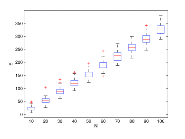
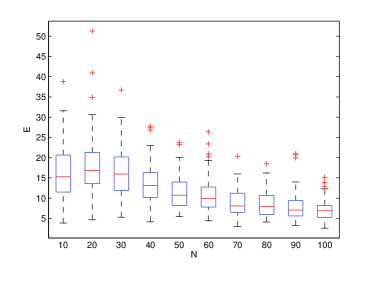
Fig. 1: Simulation results for the small diagonalizable data sets. The figures present the boxplots of the measure $E$ generated over 100 realization for [7] in the left figure and the proposed method in the right figure.

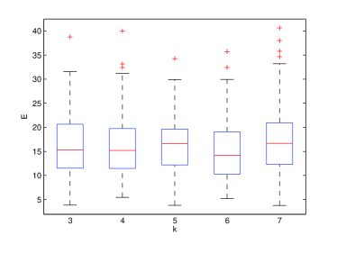
Fig. 2: Simulation results for the small diagonalizable data set of size $N=10$. The figures present the boxplots of the measure $E$ generated over 100 realization with the proposed method with dimension $k=3,4,5,6$ and $7$.

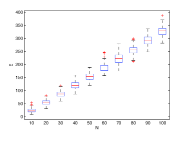
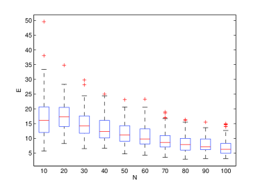
Fig. 3: Simulation results for the small approximately diagonalizable data sets. The figures present the boxplots of the measure $E$ generated over 100 realization for [7] in the left figure and the proposed method in the right figure.

5.3 Restin state fMRI experiment

In this section we evaluate the performance of the proposed joint matrices diagonalization algorithm on a resting state fMRI experiment data set [20]. Data-driven methods were successfully suggested and applied to fMRI data analysis. These methods consider the fMRI time series measured at each voxel as a mixture of signals localized in a small set of regions and other simultaneous time-varying effects. They isolate the spatial brain activity by estimating a mixing matrix and the sources that define the spatially localized neural dynamics. Most data driven fMRI analysis methods use a data matrix Y formed by vectorizing each time series observed in every voxel creating a matrix Y of dimension $N\times n$ where $n$ is the number of time points and $N$ the number of voxels, $N\gg n$.
These methods consider Y as the mixture and factorize it into latent sources through the decomposition into matrices $\textbf{Y}=\textbf{A}\textbf{X}$, a mixing matrix A and a source matrix X. Data-driven methods are suitable for the analysis of fMRI data as they minimize the assumptions on the underlying structure of the problem by decomposing the observed data based on a factor model and a specific constraint. Different constraints have led to different data-driven methods. For example, the maximum variance constraint has led to principal component analysis (PCA) [11], the independence constraint has led to independent component analysis (ICA) [14] and sparsity constraint has led to dictionary learning [13].

Recently, ICA has become a widespread data-driven method for fMRI analysis. It has led to temporal ICA (tICA, for the format of the data described above) and spatial ICA (sICA) [14]. In this experiment we applied the proposed joint diagonalization approach on twenty correlation matrices of size $939\times 939$ obtained from a data set of size $939\times 197$. This data set was constructed from the slice 41, which we know contains the activated regions of the default mode network (DMN) [20]. For comparison we used the tICA approach. We can observe from figure 4 that both the proposed approach and tICA recovered the connected regions of the DMN; the posterior cingulate cortex (PCC), medial pre-frontal cortex (MFC), and right inferior parietal lobe (IPL). Since there is no gold standard reference for DMN connectivity available, we relied on the similarity of temporal dynamics of DMN based modulation profile with PCC representative time-series. The similarity measure used was correlation and it was estimated as $>0.75$ for all the algorithms.

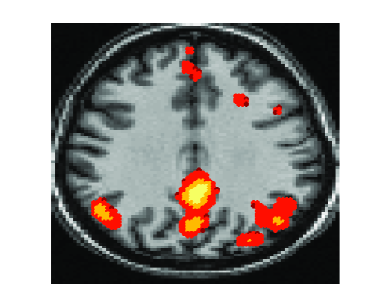
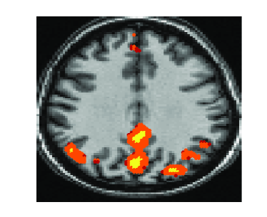
Fig. 4: Resting state fMRI results. Left: tICA [14], right: proposed approach

6 Conclusion

This paper discussed what might be termed a natural extension of the problem of joint diagonalization for the situation when the matrices under consideration are too large for standard algorithms to be applied. This extension consists of solving the problem in a subspace of small dimension, leading to the minimization of an objective function to produce an orthonormal basis of the desired subspace. A few theoretical results have been shown that characterize this optimum and establish a few equivalences. An algorithm based on a variant of subspace iteration was proposed to solve the problem and was tested on a few examples. One issue that still remains to be addressed is to show that the joint approximate eigenspace to which the algorithm converges corresponds to a dominant eigenspace for all the $C_{i}$’s. This requirement is somewhat difficult to formulate rigorously due to the approximate nature of the eigenspaces involved. In the easiest case of exact joint joint diagonalization, we would have $C_{i}Q-QD_{i}=0$ for all $i$ and we would ask that in addition $Q$ be an eigenspace associated with the $k$ dominant eigenvalues for each $C_{i}$. In the approximate case, $\|C_{i}Q-QD_{i}\|$ can only be required to be small. Then, because $Q$ is only an approximate eigenspace, it is meaningless to demand that the associated approximate eigenvalues be the largest ones for each $C_{i}$. Although the subspace iteration algorithm is likely to deliver a solution that more or less satisfies this requirement, the theoretical foundation, as well as a rigorous formulation of the result, are yet to be established.

References

- [1] K. A.-M. A. Aissa El Bey and Y. Grenier, A general framework for second-order blind separation of stationary colored sources, Signal Processing, (2008), pp. 2123–2137.
- [2] B. Afsari, Sensitivity analysis for the problem of matrix joint diagonalization, SIAM Journal on Matrix Analysis and Applications, 30 (2008), pp. 1148–1171.
- [3] A. Belouchrani, K. Abed-Meraim, J.-F. Cardoso, and E. Moulines, A blind source separation technique using second-order statistics, IEEE Transactions on Signal Processing, 45 (1997), pp. 434–444.
- [4] A. Bunse-Gerstner, R. Byers, and V. Mehrmann, Numerical methods for simultaneous diagonalization, SIAM Journal on Matrix Analysis and Applications, 14 (1993), pp. 927–949.
- [5] J. Cardoso and A. Souloumiac, Jacobi angles for simultaneous diagonalization, SIAM Journal on Matrix Analysis and Applications, 17 (1996), pp. 161–164.
- [6] J. F. Cardoso and A. Souloumiac, Blind beamforming for non-Gaussian signals, IEE Proceedings, 140 (1993), pp. 362–370.
- [7] , Jacobi angles for simultaneous diagonalization, SIAM Journal on Matrix Analysis and Applications, 17 (1996), pp. 161–164.
- [8] A. Edelman, T. A. Arias, and S. T. Smith, The geometry of algorithms with orthogonality constraints, SIAM J. Matrix Anal. Appl., 20 (1999), pp. 303–353.
- [9] E. M. Fadaili, N. Moreau, and E. Moreau, Non-orthogonal joint diagonalization/zero diagonalization for source separation based on time-frequency distributions, IEEE Transactions on Signal Processing, 55 (2007), pp. 1673–1687.
- [10] B. Flury and W. Gautschi, An algorithm for simultaneous orthogonal transformation of several positive definite symmetric matrices to nearly diagonal form, SIAM Journal on Scientific and Statistical Computing, 7 (1986), pp. 169–184.
- [11] K. J. Friston, C. D. Frith, P. F. Liddle, and R. S. J. Frackowiak, Functional connectivity: the principal component analysis of large PET data sets, Journal of Cerebral Blood Floww and Metabolism, 13 (1993), pp. 5–14.
- [12] G. H. Golub and C. F. V. Loan, Matrix Computations, 4th edition, Johns Hopkins University Press, Baltimore, MD, 4th ed., 2013.
- [13] K. Lee, S. K. Tak, and J. C. Yee, A data driven sparse GLM for fMRI analysis using sparse dictionary learning and MDL criterion, IEEE Transactions on Medical Imaging, 30 (2011), pp. 1176–1089.
- [14] M. McKeown and T. Sejnowski, Independent component analysis of fMRI data: examining the assumptions, Human Brain Mapping, 6 (1998), pp. 368–372.
- [15] B. N. Parlett, The Symmetric Eigenvalue Problem, no. 20 in Classics in Applied Mathematics, SIAM, Philadelphia, 1998.
- [16] Y. Saad, Numerical Methods for Large Eigenvalue Problems- Classics in Appl. Math., SIAM, Philadelpha, PA, 2011.
- [17] Y. Saad, Analysis of subspace iteration for eigenvalue problems with evolving matrices, SIAM Journal on Matrix Analysis and Applications, - (2016). To appear.
- [18] A. H. Sameh and Z. Tong, The trace minimization method for the symmetric generalized eigenvalue problem, J. Comput. Appl. Math., 123 (2000), pp. 155–175.
- [19] A. H. Sameh and J. A. Wisniewski, A trace minimization algorithm for the generalized eigenvalue problem, SIAM Journal on Numerical Analysis, 19 (1982), pp. 1243–1259.
- [20] Z. Shehzad, A. M. Kelly, P. T. Reiss, D. G. Gee, K. Gotimer, L. Q. Uddin, S. Lee, D. S. Margulies, A. K. Roy, B. B. Biswal, E. Petkova, F. X. Castellanos, and M. Milham, The resting brain: unconstrained yet reliable, Cerebral Cortex, (2009), pp. 2209–2229.
- [21] A. Souloumiac, Nonorthognal joint diagonalization by combining Givens and hyperbolic rotations, IEEE Transactions on Signal Processing, 57 (2009), pp. 2222–2231.
- [22] G. W. Stewart, Matrix Algorithms II: Eigensystems, SIAM, Philadelphia, 2001.
- [23] F. J. Theis, Colored subspace analysis: Dimension reduction based on a signal’s autocorrelation structure, IEEE Transactions on Circuits and Systems I: Regular Papers, 57 (2010), pp. 1463–1474.
- [24] A.-J. van der Veen, Joint diagonalization via subspace fitting techniques, in Acoustics, Speech, and Signal Processing, 2001. Proceedings. (ICASSP ’01). 2001 IEEE International Conference on, vol. 5, 2001, pp. 2773–2776 vol.5.
- [25] R. Vollgraf and K. Obermayer, Quadratic optimization for simultaneous matrix diagonalization, IEEE Transactions on Signal Processing, 54 (2006), pp. 3270–3278.
- [26] R. Vollgraf, M. Setter, and K. Obermayer, Convolutive decorrelation procedures for blind source separation, In Proceedings of the 2nd International Workshop on Indepdendent Component Analysis (ICA), (2000), pp. 515–520.
- [27] A. Yeredor, Blind source separation via the second characteristic function, Signal Processing, 80 (2000), pp. 897–902.
- [28] , Non-orthogonal joint diagonalization in the least-square sense with application in blind source separation, IEEE Transactions on Signal Processing, 50 (2002), pp. 1545–1553.