Implications of first neutrino-induced nuclear recoil measurements in direct detection experiments

Abstract

PandaX-4T and XENONnT have recently reported the first measurement of nuclear recoils induced by the ⁸B solar neutrino flux, through the coherent elastic neutrino-nucleus scattering (CE$\nu$NS) channel. As long anticipated, this is an important milestone for dark matter searches as well as for neutrino physics. This measurement means that these detectors have reached exposures such that searches for low mass, $\lesssim 10$ GeV dark matter cannot be analyzed using the background-free paradigm going forward. It also opens a new era for these detectors to be used as neutrino observatories. In this paper we assess the sensitivity of these new measurements to new physics in the neutrino sector. We focus on neutrino non-standard interactions (NSI) and show that—despite the still moderately low statistical significance of the signals—these data already provide valuable information. We find that limits on NSI from PandaX-4T and XENONnT measurements are comparable to those derived using combined COHERENT CsI and LAr data, as well as those including the latest Ge measurement. Furthermore, they provide sensitivity to pure $\tau$ flavor parameters that are not accessible using stopped-pion or reactor sources. With further improvements of statistical uncertainties as well as larger exposures, forthcoming data from these experiments will provide important, novel results for CE$\nu$NS-related physics.

I Introduction

PandaX-4T Bo et al. (2024) and XENONnT Aprile et al. (2024) have recently reported the detection of coherent elastic neutrino-nucleus scattering (CE$\nu$NS) induced by ⁸B solar neutrinos. Due to their low energy thresholds and large active volumes these experiments identify the ⁸B component of the solar neutrino flux at a significance level of the order of $2\sigma$. This is the first detection of CE$\nu$NS from an astrophysical source, complementing the recent detections from the stopped-pion source by the COHERENT experiment Akimov et al. (2017, 2019); Adamski et al. (2024). Further, this detection probes the CE$\nu$NS cross section at characteristic neutrino energy scales lower than that probed by COHERENT and with a new material target.

The detection of solar neutrinos at dark matter (DM) detectors such as PandaX-4T and XENONnT is a milestone in neutrino physics Monroe and Fisher (2007); Vergados and Ejiri (2008); Strigari (2009); Billard et al. (2014); O’Hare (2021). It represents an important step in the continuing development of the solar neutrino program, dating back to over half of a century. From the perspective of solar neutrino physics, it is the second pure neutral current channel detection of the solar neutrino flux, complementing the SNO neutral current detection of the flux using a deuterium target Aharmim et al. (2013). Its observation was anticipated long time ago to be not only a challenge for DM searches, but also an opportunity for a better understanding of neutrino properties and searches of new physics Aalbers et al. (2023).

The detection of ⁸B neutrinos via CE$\nu$NS has important implications more broadly for neutrino physics, astrophysics, and DM. This detection has the potential to provide information on the properties of the solar interior Cerdeno et al. (2018). It also has the potential to probe new physics in the form of non-standard neutrino interactions (NSI) Dutta et al. (2017); Aristizabal Sierra et al. (2018, 2019a); Dutta and Strigari (2019), sterile neutrinos Billard et al. (2015); Alonso-González et al. (2023), neutrino electromagnetic properties Aristizabal Sierra et al. (2020a, 2022a); Cadeddu et al. (2021); Giunti and Ternes (2023) or new interactions involving light mediators Aristizabal Sierra et al. (2019a, 2020b). Detection of solar neutrinos via CE$\nu$NS also is important for interpreting the possible detection of low mass, $\lesssim 10$ GeV, dark matter Dent et al. (2017); Aristizabal Sierra et al. (2022b). A detailed understanding of this signal is of paramount importance for the interpretation of future data. The identification of a possible WIMP signal requires a thorough understanding of neutrino-induced nuclear recoils.

In this paper, we examine the sensitivity of the PandaX-4T and XENONnT data to NSI. We show that even with this early data these measurements are already capable of providing competitive bounds. In particular, because of neutrino flavor conversion, these measurements are sensitive to all neutrino flavors and so open flavor channels not accessible in CE$\nu$NS experiments relying on $\pi^{+}$ decay-at-rest or reactor neutrino fluxes. Thus from this point of view these experiments are very unique.

The reminder of this paper is organized as follows. In Sec. II we discuss the Standard Model (SM) CE$\nu$NS cross section, define the parameters we use in our calculation and briefly discuss the experimental input employed. In Sec. II we provide a detailed discussion of NSI effects in both propagation and detection. To do so we rely on the two-flavor approximation, which provides rather reliable results up to corrections of $\sim 10\%$ . In Sec. IV, after briefly discussing the main features of both PandaX-4T and XENONnT data, we present the results of our analysis. Finally, in Sec. V we summarize and present our conclusions. In App. A we provide a summary of NSI limits arising from the one-parameter analysis.

II CE$\nu$NS cross section, ⁸B solar neutrino flux, event rates and experimental input

In the SM, at tree-level the CE$\nu$NS cross section is has no lepton flavor dependence Freedman (1974), with flavor-dependent corrections appearing at the one-loop level Sehgal (1985); Tomalak et al. (2021); Mishra and Strigari (2023). At tree level the scattering cross section reads Freedman (1974)

$$\frac{d\sigma}{dE_{r}}=\frac{G_{F}^{2}}{2\pi}\,Q^{2}_{W}\,m_{N}\left(2-\frac{m_{N}E_{r}}{E_{\nu}^{2}}\right)F^{2}_{W}(E_{r})\ .$$ (1)

For the nuclear mass, $m_{N}$, we use the averaged mass number $\langle A\rangle=\sum_{i=1}^{9}X_{i}A_{i}$, where $i$ runs over the nine stable xenon isotopes and $X_{i}$ refers to $i$-th isotope natural abundance. $Q_{W}$ refers to the weak charge and determines the strength at which the $Z$ gauge boson couples to the nucleus. At tree-level and neglecting $q^{2}$ dependent terms ($q$ referring to the transferred momentum) the weak charge is entirely determined by the vector neutron and proton couplings

$$Q_{W}=Zg^{p}_{V}+N\,g^{n}_{V}\ ,$$ (2)

with $Z=54$ referring to the nucleus atomic number and $N=(\langle A\rangle-Z)$ to the number of neutrons. The nucleon couplings are in turn given by the fundamental electroweak neutral current up and down couplings: $g_{V}^{p}=1/2-2\sin^{2}\theta_{W}$ and $g_{V}^{n}=-1/2$. Because of the value of the weak mixing angle, $g_{V}^{n}$ exceeds $g_{V}^{p}$ by more than a factor 20. Thus, up to small corrections the total cross section scales as $N^{2}=(A-Z)^{2}$.

Effects due to the finite size of the nucleus are parameterized in terms of the weak-charge form factor, $F_{W}$, for which different parametrizations can be adopted. However, given the energy scale of solar neutrinos these finite size nuclear effects are small, not exceeding more than a few percent regardless of the parametrization Aristizabal Sierra et al. (2019b); Aristizabal Sierra (2023). Although of little impact, our calculation does include the weak-charge form factor. We have adopted the Helm parametrization Helm (1956) along with $R_{n}=R_{C}+0.2\,\text{fm}$, with $R_{C}$ calculated by averaging the charge radius of each of the nine xenon stables isotopes over their natural abundance.

Flux	Normalization [$\text{cm}^{-2}\text{s}^{-1}$]	End-point [MeV]
$pp$	$5.98\times 10^{10}$	$0.40$
${}^{7}\text{Be}$	$4.93\times 10^{9}$	$0.38,0.86$
$pep$	$1.44\times 10^{8}$	$1.44$
${}^{13}\text{N}$	$2.78\times 10^{8}$	$1.20$
${}^{15}\text{O}$	$2.05\times 10^{8}$	$1.73$
${}^{17}\text{F}$	$5.29\times 10^{6}$	$1.74$
${}^{8}\text{B}$	$5.46\times 10^{6}$	$16.0$
$hep$	$7.98\times 10^{3}$	$18.7$

Table 1: Neutrino flux normalization as recommended in Ref. Baxter et al. (2021) and inline with the B16(GS98) SSM. For detection only ⁸B matters. For propagation we include the whole spectrum.

⁸B electron neutrinos are produced in $\beta^{+}$ decay processes: ${}^{8}\text{B}\to\text{Be}^{*}+e^{+}+\nu_{e}$. The features of the spectrum as well as its normalization is dictated by the Standard Solar Model (SSM). In our analysis we use the values predicted by the B16(GS98) SSM Vinyoles et al. (2017). The distribution of ⁸B neutrino production from the B16(GS98) SSM peaks at around $5\times 10^{-2}\,R_{\odot}$ and ceases to be efficient at $0.1\,R_{\odot}$, where the distribution fades away. For the calculation of event rates only the ⁸B neutrino flux is required. For the calculation of propagation effects (matter effects), however, we require all possible fluxes. In all cases we adopt neutrino spectra normalization as recommended for reporting results for direct DM searches Baxter et al. (2021), which are inline with those predicted by the B16(GS98) SSM. The values for those normalization factors along with the kinematic end-point energies for all fluxes are shown in Tab. 1.

Calculation of differential event rate spectra follows from convoluting the CE$\nu$NS differential cross section in Eq. (1) with the ⁸B spectral function, namely

$$\frac{dR}{dE_{r}}=\frac{\varepsilon\,N_{A}}{m_{\text{mol}}^{\text{Xe}}}N_{{}^{8}\text{B}}\int_{E_{\nu}^{\text{min}}}^{E^{\text{max}}_{\nu}}\frac{d\Phi_{{}^{8}\text{B}}}{dE_{\nu}}\frac{d\sigma}{dE_{r}}dE_{\nu}\ .$$ (3)

Here $\varepsilon$ refers to exposure measured in tonne-year, $N_{A}$ is the Avogadro number in 1/mol units, $m_{\text{mol}}^{\text{Xe}}=131.3\times 10^{-3}\text{kg/mol}$, $N_{{}^{8}\text{B}}$ the ⁸B flux normalization from Tab. 1, $E^{\text{min}}_{\nu}=\sqrt{m_{N}E_{\nu}/2}$ and $E^{\text{max}}_{\nu}$ the kinematic end-point of the ⁸B spectrum from Tab. 1 as well. Eq. (3) is valid in the SM, where the CE$\nu$NS differential cross section is flavor universal at tree level. If either through one-loop corrections or new physics the cross section becomes flavor dependent, then the integrand should involve the probability associated with each neutrino flavor (see Sec. III.2 for a more detailed discussion). The event rate follows from integration of Eq. (3) over recoil energies, with the experimental acceptance $\mathcal{A}(E_{r})$ fixed according to the PandaX-4T or XENONnT data sets. Generically it reads

$$R=\int_{E_{r}^{\text{min}}}^{E_{r}^{\text{max}}}\mathcal{A}(E_{r})\frac{dR}{dE_{r}}dE_{r}\ .$$ (4)

PandaX-4T perform two types of analyses on their data. First, they perform a combined S1/S2 analysis, in which a neutrino signal event is identified via both prompt scintillation and secondary ionization signals from the nuclear recoil (paired signal). The low energy threshold for this analysis is set by the S1 signal, which in terms of nuclear recoil energy is $\sim 1.1$ keV. The second analysis is an S2 only analysis, in which only the ionization component is used as the signal of an event (US2 signal). In this case, the nuclear recoil threshold is lower, $\sim 0.3$ keV, but the trade-off is an increase in the backgrounds for this sample.

PandaX-4T present data from two runs: their commissioning run, which they call Run0, and their first science run, which they call Run1. For the paired data set, the exposure is 1.25 tonne-year, and for the US2, the exposure is 1.04 tonne-year. Using a maximum likelihood analysis, PandaX-4T finds a best fitting ⁸B event rate from the US2 sample of $75\pm 28$ and a paired event rate of $3.5\pm 1.3$.

The XENONnT collaboration combined two separate analyses, labelled SR0 and SR1, which when combined amount to an exposure of 3.51 tonne-year. They present acceptances for both an S1 only and an S2 only analysis. For the primary analysis, XENONnT combine the acceptances for S1 and S2 (with a resulting 0.5 keV threshold), and, for this combined exposure, they quote a best fit event rate of $10.7_{-4.2}^{+3.7}$. They point out that this result is in close agreement with: (i) Expectations from the measured solar ⁸B neutrino flux from SNO, (ii) the theoretical CE$\nu$NS cross section with xenon nuclei, (iii) calibrated detector response to low-energy nuclear recoils. For the expected event rate, they find $11.9^{+4.5}_{-4.2}$. Calculation of the $Z$-score—assuming these results to be independent—yields $0.2\,\sigma$. Thus using either in our statistical procedure produces no sizable deviation in the final results. Tab. 2 summarizes the detector parameter configurations along with the signals we have employed.

Data set	Exp [tonne-year]	$E_{r}^{\text{min,max}}$ [keV]	Signal
PandaX-4T (paired)	1.25	1.1/3.0	$3.5\pm 1.3$
PandaX-4T (US2)	1.04	0.3/3.0	$75\pm 28$
XENONnT	3.51	0.5/3.0	$10.7\pm 3.95$

Table 2: PandaX-4T (paired and US2) and XENONnT parameter detector configurations used in the NSI statistical analysis. Values taken from Refs. Bo et al. (2024); Aprile et al. (2024).

III Neutrino non-standard interactions

In addition to loop-level corrections, flavor-dependence in the CE$\nu$NS cross section may also be introduced through neutrino NSI Barranco et al. (2005). The effective Lagrangian accounting for the new vector interactions can be written as

$$\mathcal{L}_{\text{NSI}}=-\sqrt{2}G_{F}\sum_{\begin{subarray}{c}i=e,\mu,\tau\\ q=u,d\end{subarray}}\overline{\nu}_{i}\,\gamma_{\mu}P_{L}\epsilon_{ij}^{q}\,\nu_{j}\,\overline{q}\gamma^{\mu}q\ ,$$ (5)

where the $\epsilon_{ij}^{q}$ parameters determine the strength of the effective interaction with respect to the SM strength. Neutrino NSI affect neutrino production, propagation and detection. Since production takes place through charged-current (CC) processes, effects in production are small . Effects on propagation and detection, being due to neutral current, can instead be potentially large. Thus we consider only those two. Propagation effects arise from forward scattering processes which induce matter potentials proportional to the number density of the scatterers. So in addition to the SM matter potential, the new interaction—being of vector type—induces additional matter potentials that affect neutrino propagation and thus neutrino flavor conversion. Detection, instead, becomes affected because of the impact of the new effective interaction on the CE$\nu$NS cross section. All in all, NSI effects on solar neutrinos may be prominent in propagation $\oplus$ detection.

Neutrino NSI are constrained by a variety of experimental searches. Here we provide a summary of the main constraints, which does not aim at being complete but rather to provide a general picture of what has been done (for a more detailed account see e.g. Ref. Farzan and Tortola (2018)). First of all, global analysis of oscillation data imply tight constraints on the size and flavor structure of matter effects. Thus, those constraints can be translated into limits on NSI parameters Gonzalez-Garcia et al. (2011); Gonzalez-Garcia and Maltoni (2013). Limits involving global analysis of oscillation data combined with CE$\nu$NS measurements have been also derived Esteban et al. (2018); Coloma et al. (2023). Constraints from CE$\nu$NS data alone, for which only effects on detection apply, have been analyzed using both CsI data releases along with LAr data in Ref. De Romeri et al. (2023), and also the most recent measurement with germanium in Ref. Liao et al. (2024). Further constraints from monojets and missing energy searches at the LHC exist Friedland et al. (2012); Buarque Franzosi et al. (2016). Involving electrons and at early times, the new interaction can keep neutrinos in thermal contact with electrons and positrons below $\sim 1\,$MeV. Requiring small departures from this value leads to cosmological constraints de Salas et al. (2021a). In supernovæ, neutrino NSI have as well been considered in e.g. Refs. Esteban-Pretel et al. (2007); Jana and Porto (2024).

In what follows we describe their effects in propagation and in detection. To do so we rely on the two-flavor approximation, well justified up to corrections of the order of $10\%$ because of $\Delta m_{12}^{2}/\Delta m_{13}^{2}\ll 1$ and $\sin^{2}\theta_{13}\ll 1$ de Salas et al. (2021b). And rather than including the data and constraints discussed above, we focus only on the constraints implied by PandaX-4T and XENONnT.

III.1 Neutrino NSI: Propagation effects

Electron neutrinos are subject to flavor conversion in the Sun, governed by the vacuum and matter Hamiltonians

$$i\frac{d}{dr}|\boldsymbol{\nu}\rangle=\left[\frac{1}{2E_{\nu}}\boldsymbol{U}\;\boldsymbol{H_{\text{vac}}}\;\boldsymbol{U}^{\dagger}+\boldsymbol{H_{\text{mat}}}\right]|\boldsymbol{\nu}\rangle\ .$$ (6)

Here $|\boldsymbol{\nu}\rangle^{T}=|\nu_{e},\nu_{\mu},\nu_{\tau}\rangle^{T}$ refers to the neutrino flavor eigenstate basis, $r$ to the neutrino propagation path, $\boldsymbol{U}=U_{23}U_{13}U_{12}\equiv U(\theta_{23})U(\theta_{13})U(\theta_{12})$ is the $3\times 3$ leptonic mixing matrix parametrized in the standard way, $\boldsymbol{H_{\text{vac}}}=\text{diag}(0,\Delta m_{21}^{2},\Delta m_{31}^{2})$ and in the absence of NSI the matter Hamiltonian is given by $\boldsymbol{H_{\text{mat}}}=\sqrt{2}G_{F}\,n_{e}(r)\text{diag}(1,0,0)$. Note that because of matter potentials neutrino flavor evolution is more conveniently followed in the flavor basis.

As previously pointed out, the presence of neutrino NSI induce new matter potential terms that modify the flavor evolution equation, namely

$$i\frac{d}{dr}|\boldsymbol{\nu}\rangle=\left[\frac{1}{2E_{\nu}}\boldsymbol{U}\;\boldsymbol{H_{\text{vac}}}\;\boldsymbol{U}^{\dagger}+\sqrt{2}G_{F}n_{e}(r)\sum_{f=e,u,d}\boldsymbol{\varepsilon^{f}}\right]|\boldsymbol{\nu}\rangle\ ,$$ (7)

where the NSI coupling matrices $\varepsilon^{f}$ involves the quark relative abundances in addition to the parameters entering in Eq. (17):

$$\boldsymbol{\varepsilon^{f}}=\begin{pmatrix}1+\varepsilon_{ee}^{f}&\varepsilon_{e\mu}^{f}&\varepsilon_{e\tau}^{f}\\ \varepsilon_{e\mu}^{f}&\epsilon_{\mu\mu}^{f}&\varepsilon_{\mu\tau}^{f}\\ \varepsilon_{e\tau}^{f}&\varepsilon_{\mu\tau}^{f}&\varepsilon_{\tau\tau}^{f}\\ \end{pmatrix}\ .$$ (8)

Explicitly, $\varepsilon_{ij}^{f}(r)=Y_{f}(r)\epsilon_{ij}^{f}$ ($f=e,u,d$) with $Y_{f}(r)=n_{f}(r)/n_{e}(r)$. The up- and down-quark relative abundances are written in terms of the neutron relative abundance $Y_{u}=2+Y_{n}$ and $Y_{d}=1+2Y_{n}$, with the neutron number density calculated from the ⁴He and ¹H mass fractions.

A three-flavor analysis of NSI matter effects demands numerical integration of Eq. (7) for each point in the NSI parameter space. However, an analytical, less CPU expensive and yet precise approach can be adopted in the so-called mass dominance limit $\Delta m_{13}^{2}\to\infty$ Gonzalez-Garcia and Maltoni (2013). In this approximation, neutrino propagation is properly described in the basis $|\widetilde{\nu}\rangle=\mathcal{U}^{T}|\nu\rangle\equiv U_{13}^{T}U_{23}^{T}|\nu\rangle$ (propagation basis). Up to corrections of the order of $\sin\theta_{13}$, the propagating neutrino states are: A mainly electron neutrino state ($\tilde{\nu}_{e}$), a superposition of muon and tau neutrinos state ($\tilde{\nu}_{\mu}$) and its orthogonal counterpart ($\tilde{\nu}_{\tau}$). With these considerations, only $\tilde{\nu}_{e}$ and $\tilde{\nu}_{\mu}$ have sizable mixing. Mixing with $\tilde{\nu}_{\tau}$ for neutrino energies of the order of $10\,$MeV and average SSM quark number densities does not exceed $3\times 10^{-2}\times\epsilon_{ij}^{q}$ Aristizabal Sierra et al. (2018). With $\tilde{\nu}_{\tau}$ “decoupled” from mixing, flavor conversion becomes then a two-flavor problem that can be entirely treated at the analytic level.

In two-flavor approximation, the survival probability is given by $\mathcal{P}_{ee}(E_{\nu},r)$ Gonzalez-Garcia and Maltoni (2013)

$$\mathcal{P}_{ee}(E_{\nu},r)=\cos^{4}\theta_{13}\,\mathcal{P}_{\text{eff}}(E_{\nu},r)+\sin^{4}\theta_{13}\ ,$$ (9)

where the $r$ dependence is introduced by the effective probability given by Parke (1986)

$$\mathcal{P}_{\text{eff}}(E_{\nu},r)=\frac{1+\cos 2\theta_{M}(r)\cos 2\theta_{12}}{2}\ .$$ (10)

Here $\theta_{M}(r)$ is the mixing angle in matter and adiabatic propagation has been assumed, thus implying a rather suppressed level-crossing probability ($P_{c}\to 0$). With neutrino oscillation data taken from Ref. de Salas et al. (2021b), calculation of the survival probability in Eq. (9) then reduces to the determination of $\theta_{M}$. To do so the following $2\times 2$ Hamiltonian has to be diagonalized

$$\boldsymbol{H}=\frac{1}{4E_{\nu}}\begin{pmatrix}-\Delta m_{21}^{2}\cos 2\theta_{12}+A&\Delta m_{21}^{2}\sin 2\theta_{12}+B\\ \Delta m_{21}^{2}\sin 2\theta_{12}+B&\Delta m_{21}^{2}\cos 2\theta_{12}-A\end{pmatrix}\ .$$ (11)

In this expression the $A$ and $B$ terms in the diagonal and off-diagonal entries are given by

$$A =4\sqrt{2}E_{\nu}G_{F}n_{e}(r)\left[\frac{\cos^{2}\theta_{13}}{2}-Y_{q}(r)\varepsilon_{D}^{q}\right]\ ,$$

$$B =4\sqrt{2}E_{\nu}G_{F}n_{e}(r)Y_{q}(r)\varepsilon_{N}^{q}\ ,$$ (12)

from where it can be seen that in the limit $\epsilon_{ij}^{q}=0$ and $\cos\theta_{13}=0$, $A$ reduces to the SM term and $B$ vanishes. The parameters $\varepsilon_{D}$ and $\varepsilon_{N}$ result from the rotation from the flavor to the propagation basis and read Gonzalez-Garcia and Maltoni (2013):

$$\varepsilon_{D}^{q} =-\frac{c_{13}^{2}}{2}\epsilon_{ee}^{q}+\frac{\left[c_{13}^{2}-\left(s_{23}^{2}-s_{13}^{2}c_{23}^{2}\right)\right]}{2}\epsilon_{\mu\mu}^{q}+\frac{\left(s_{23}^{2}-c_{23}^{2}s_{13}^{2}\right)}{2}\epsilon_{\tau\tau}^{q}+s_{13}c_{13}s_{23}\epsilon_{e\mu}^{q}+s_{13}c_{13}c_{23}\epsilon_{e\tau}^{q}-(1+s^{2}_{13})\,c_{23}s_{23}\epsilon_{\mu\tau}^{q}\ ,$$ (13)

$$\varepsilon_{N}^{q} =-s_{13}c_{23}s_{23}\epsilon_{\mu\mu}^{q}+s_{13}c_{23}s_{23}\epsilon_{\tau\tau}^{q}+c_{13}c_{23}\epsilon_{e\mu}^{q}-c_{13}s_{23}\epsilon_{e\tau}^{q}+s_{13}\left(s_{23}^{2}-c_{23}^{2}\right)\epsilon_{\mu\tau}^{q}\ ,$$ (14)

where $c_{ij}\equiv\cos\theta_{ij}$ and $s_{ij}\equiv\sin\theta_{ij}$. The mixing angle in matter thus can be written as

$$\cos 2\theta_{M}(r)=\frac{\Delta m_{12}^{2}\cos 2\theta_{12}-A}{\sqrt{\left(\Delta m_{12}^{2}\cos 2\theta_{12}-A\right)^{2}+\left(\Delta m_{12}^{2}\sin 2\theta_{12}+B\right)^{2}}}\ .$$ (15)

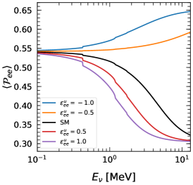
Figure 1: Averaged survival probability as a function of neutrino energy for the case in which only $\epsilon_{ee}^{u}$ has a non-vanishing value. This graph aims only at illustrating the impact of neutrino NSI on neutrino propagation in the Sun. The different features are related with the kinematic end-points where certain neutrino fluxes fade away [see Tab. 1 along with Eq. (16)].

Eqs. (9) and (10) combined with Eqs. (III.1)-(15) allow the determination of $\mathcal{P}_{ee}(E_{\nu},r)$ in terms of neutrino oscillation parameters, electron and quark number densities and NSI parameters. The averaged survival probability is then obtained by integrating over $r$ taking into account the distribution of neutrino production in the Sun Gonzalez-Garcia and Maltoni (2013):

$$\langle\mathcal{P}_{ee}(E_{\nu})\rangle=\frac{\sum_{\alpha}\Phi_{\alpha}(E_{\nu})\int_{0}^{1}\,dr\rho(r)\,\mathcal{P}_{ee}(E_{\nu},r)}{\sum_{\alpha}\Phi_{\alpha}(E_{\nu})}\ ,$$ (16)

where $\Phi_{\alpha}(E_{\nu})$ refers to the $\alpha$ component of the solar neutrino flux (with $\alpha$ running over all components) and $\rho_{\alpha}(r)$ to the distribution of neutrino production. For illustration (and only with that aim), in Fig. 1 we show an example of the averaged survival probability as a function of the neutrino energy for the case in which all couplings but $\epsilon_{ee}^{u}$ vanish. As can be seen, the new interaction can either enhance or deplete neutrino flavor conversion depending on its strength and on whether it reinforces or weakens the SM matter potential. With propagation effects already discussed and summarized in Eq. (16) we now turn to the discussion of detection effects.

III.2 Neutrino NSI: Detection effects

For consistency, the same basis used for neutrino propagation should be used in neutrino detection as well. In doing so the effective Lagrangian in Eq. (17) reads

$$\mathcal{L}_{\text{NSI}}=-\sqrt{2}G_{F}\sum_{\begin{subarray}{c}i=e,\mu,\tau\\ q=u,d\end{subarray}}\overline{\widetilde{\nu}}_{i}\,\gamma_{\mu}P_{L}\widetilde{\epsilon}_{ij}^{q}\,\widetilde{\nu}_{j}\,\overline{q}\gamma^{\mu}q\ ,$$ (17)

where $\widetilde{\epsilon}^{q}=\mathcal{U}^{T}\epsilon^{q}\mathcal{U}\equiv U_{13}^{T}U_{23}^{T}\epsilon^{q}U_{23}U_{13}$. With the couplings rotated this way the weak-charge in the CE$\nu$NS cross section in Eq. (1) becomes lepton flavor dependent, with the weak-charge in initial-state flavor $i$ given by

$$Q_{\nu_{i}}^{2}=\left[+N\left(g_{V}^{n}+\widetilde{\epsilon}_{ii}^{u}+2\widetilde{\epsilon}_{ii}^{d}\right)+Z\left(g_{V}^{p}+2\widetilde{\epsilon}_{ii}^{u}+\widetilde{\epsilon}_{ii}^{d}\right)\right]^{2}+\sum_{j\neq i}\left[N\left(\widetilde{\epsilon}_{ij}^{u}+2\widetilde{\epsilon}_{ij}^{d}\right)+Z\left(2\widetilde{\epsilon}_{ij}^{u}+\widetilde{\epsilon}_{ij}^{d}\right)\right]^{2}\ .$$ (18)

The couplings entering in the weak charge can be readily calculated from their definition, with the rotation matrices parametrized for a passive rotation: $\widetilde{\epsilon}_{ij}^{q}=\sum_{k,\ell}\mathcal{U}_{ki}\varepsilon^{q}_{k\ell}\mathcal{U}_{\ell j}$. The effects of the NSI are then clear. By modifying the weak-charge the new interactions can either enhance of deplete the expected reaction rate. Eq. (18) shows that diagonal couplings can produce constructive or destructive interference, while off-diagonal couplings cannot. Note that a proper definition of the flavor basis is, in principle, not possible in the presence of flavor off-diagonal NSI parameters. Strictly speaking then a consistent treatment of such cases requires a density matrix formulation for the calculation of event rates Coloma et al. (2023). Arguably, however, differences between the “standard” approach and the latter are expected to be small provided the off-diagonal parameters are suppressed. That this is the case is somehow expected from data, which do not sizably deviates from the SM expectation. Thus, we adopt the standard procedure regardless of the flavor structure of the parameters considered.

In the two-flavor approximation, two neutrino flavors reach the detector: $\widetilde{\nu}_{e}$ and $\widetilde{\nu}_{\mu}$. Lepton flavor composition of the final state, however, depends on the lepton flavor structure of the interaction. In full generality, the differential event rate is then written as follows

$$\frac{dR}{dE_{r}}=\sum_{k=e,\mu,\tau}\left(\frac{dR_{ek}}{dE_{r}}+\frac{dR_{\mu k}}{dE_{r}}\right)\ .$$ (19)

Here the flavored differential event rates are obtained from Eq. (3) by trading $Q_{W}\to Q_{\nu_{i}}$ and by taking into account the survival probability, $\langle\mathcal{P}_{ee}\rangle$, in the first term as well as the oscillation probability to the $\widetilde{\nu}_{\mu}$ state, $1-\langle\mathcal{P}_{ee}\rangle$, in the second term. Thus, in the first (second) differential event rate in Eq. (19) couplings $\widetilde{\epsilon}_{ek}^{q}$ ($\widetilde{\epsilon}_{\mu k}^{q}$) contribute. These couplings are a superposition of the NSI parameters we started with, so in a single-parameter analysis (which we adopt in the first part in Sec. IV) a non-vanishing unrotated NSI parameter can imply the presence of multiple rotated parameters at the cross section level.

IV Analysis and results

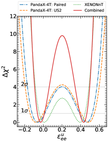
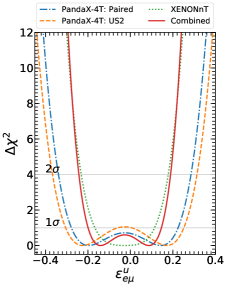
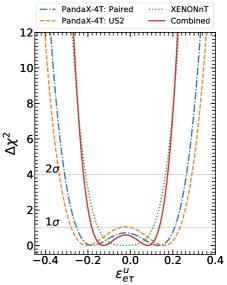
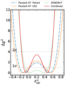
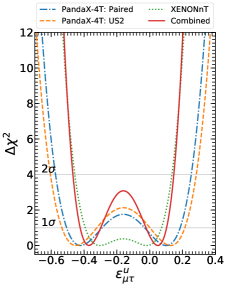
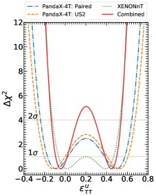
Figure 2: Dependence of the $\Delta\chi^{2}$ function on the up-quark NSI parameters for the PandaX-4T [paired and unpaired ionization-only signals (US2)] as well as for XENONnT data sets. Results for the combined analysis are shown as well. The $1\sigma$ and $2\sigma$ confidence level values (horizontal lines) are shown to facilitate reading.

The general problem of assessing the impact of neutrino NSI parameters in neutrino-nucleus event rates involves twelve independent couplings. It is of course a very CPU expensive problem, but not only that. With only a few observables to rely upon, little can be said in the most general case. For practical reasons and as well to make contact with previous analysis, we adopt a single-parameter approach. Towards the end of this section we consider the three lepton flavor diagonal two-parameter cases ($\epsilon_{ee}^{u}$,$\epsilon_{ee}^{d}$), ($\epsilon_{\mu\mu}^{u}$,$\epsilon_{\mu\mu}^{d}$) and ($\epsilon_{\tau\tau}^{u}$,$\epsilon_{\tau\tau}^{d}$); as well to make contact with what has been done previously in the literature (the $e$ and $\mu$ cases motivated by previous COHERENT data analysis). It is worth mentioning that because of neutrino flavor mixing multi-ton DM detectors are sensitive to $\tau$ flavor, which neither reactor nor stopped-pion sources are. From this point of view these measurements are unique.

We start with $u$-quark couplings and proceed by defining a simple $\chi$-square test

$$\chi^{2}=\left(\frac{R_{\text{Exp}}-R_{\text{SM+NSI}}}{\sigma_{\text{Exp}}}\right)^{2}\ ,$$ (20)

where $R_{\text{Exp}}$ refers to PandaX-4T and XENONnT event rates central values and (see Tab. 2) and $R_{\text{SM+NSI}}$ to the SM events rates including as well NSI contributions. Though oversimplified, such $\chi$-square statistic allows to capture the main features of the data sets and their sensitivity to NSI parameters. Results are shown in Fig. 2. First of all, in all cases and with all data sets two minima are found. This result follows from allowing the NSI parameter to have positive and negative values. Because of this range, as we have already pointed out, event rates are symmetric around a small value. Experimental results are thus reproduced in two non-overlapping regions of parameter space.

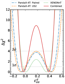
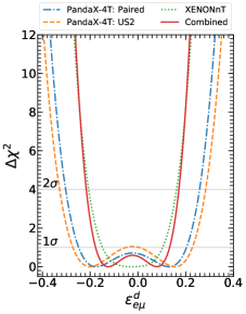
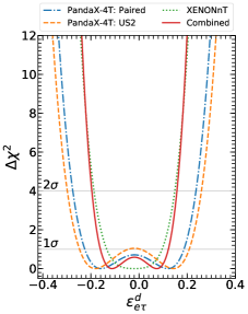
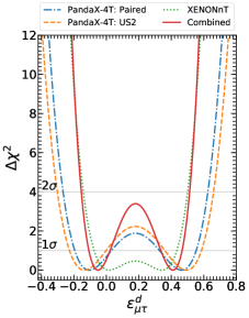
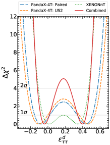
Figure 3: Dependence of the $\Delta\chi^{2}$ function on the down-quark NSI parameters for the PandaX-4T [paired and unpaired ionization-only signals (US2)] as well as for XENONnT data sets. Results for the combined analysis are shown as well. The $1\sigma$ and $2\sigma$ confidence level values (horizontal lines) are shown to facilitate reading.

One can see, however, the regions tend to be less pronounced for the XENONnT analysis, regardless of the NSI parameter. Statistical uncertainties are of the order of $\sim 37\%$ in all cases, so they cannot account for this behavior. We thus understand this tendency to be related with measured values and the SM expectation, as we now discuss. We find for the SM predicted values 2.4:46.8:11.3 events for paired:US2:XENONnT. Experimental ranges are on the other hand [2.2,4.8]:[47.0,103.0]:[6.7,14.6] for paired:US2:XENONnT. So, PandaX-4T results tend to prefer values above the SM prediction, while the SM value expected at XENONnT is well within the measured interval. In fact, the expected SM value is $5\%$ away from the midrange, 10.65 events.

From the results one can see that narrower $1\sigma$ level ranges are found for flavor-diagonal parameters. Results for flavor off-diagonal couplings are, instead, wider. This is as well expected. At the cross section level flavor-diagonal contributions add/subtract linearly to the SM contribution, while flavor off-diagonal do quadratically. Since $|\epsilon_{ij}^{u}|<1.0$, the diagonal components lead to larger deviations than the off-diagonal do for larger values.

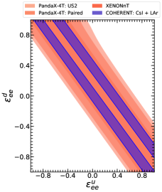
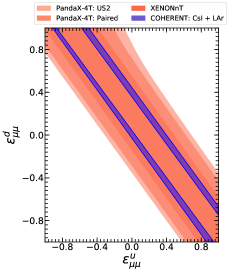
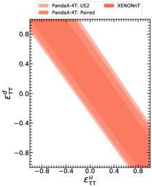
Figure 4: $\Delta\chi^{2}$ $90\%$ CL isocontours in the $\epsilon_{ee}^{u}-\epsilon_{ee}^{d}$ (left graph) and $\epsilon_{\mu\mu}^{u}-\epsilon_{\mu\mu}^{d}$ (middle graph) and $\epsilon_{\tau\tau}^{u}-\epsilon_{\tau\tau}^{d}$ (left graph) planes. Results are shown for the PandaX-4T [paired and unpaired ionization-only signals (US2)] as well as for XENONnT data sets. For comparison results from combined analysis of COHERENT CsI+LAr data De Romeri et al. (2023) are shown as well. Results for the combined analysis have a strong overlapp with those from XENONnT so are not displayed. Note that COHERENT measurements are not sensitive to $\epsilon_{\tau\tau}^{q}$ NSI parameters.

We provide as well results from a combined analysis, that we have generated by constructing a combined chi-square test $\chi^{2}_{\text{Combined}}=\chi^{2}_{\text{Paired}}+\chi^{2}_{\text{US2}}+\chi^{2}_{\text{XENONnT}}$. These results, however, should be interpreted with certain caution. Combining PandaX-4T and XENONnT this way is certainly reliable, but combining paired and US2 data sets might be not because of possible correlations. Very likely the most suitable way of combining these data sets is through a covariance matrix. However, such an analysis can only be performed with the full data sets, including backgrounds. it can be noted that the combined analysis is dominated by XENONnT data, with the reason being what we pointed out already: XENONnT measurement is more inline with the SM expectation.

Results for down-quark couplings are shown in Fig. 3. Differences between these results and those found in the up-quark case are small, a result which is also expected. From a simple inspection of Eqs. (13) and (14) one can see that at the averaged survival probability level they enter in the same functional form. Differences between up and down quarks arise only through their relative abundance, for which in the region of interest ($0.1\,R_{\odot}$) $Y_{u}$ differs by no more than $30\%$ from $Y_{d}$ Vinyoles et al. (2017). At the cross section level, the combination of down-quark couplings is different from that from the up-quark couplings [see Eq. (18)]. However, those differences are small and to a certain degree smooth out at the event rate level.

We have summarized the $1\sigma$ level ranges following from these two analyzes in Tab. 3 in App. A. It is worth comparing these results with those derived recently from a combined analysis of COHERENT data De Romeri et al. (2023). For diagonal couplings these results are rather comparable to those reported in Ref. De Romeri et al. (2023). More sizable deviations are found for off-diagonal parameters, in particular for $\epsilon_{e\mu}^{q}$ and $\epsilon_{\mu\tau}^{q}$ where the COHERENT combined analysis leads to constraints that exceed those found here by about $20\%-50\%$. Thus, these data sets already provide limits that are comparable with those derived using COHERENT data. Expectations are then that with forthcoming measurements sensitivities to possible new physics in the neutrino sector will improve. Most relevant is the fact that contrary to data coming from stopped-pion sources and/or reactors, measurements from solar neutrino data are sensitive to pure $\tau$ flavor parameters.

Finally, results for the two-parameter analysis are shown in Fig. 4. Overlaid are those derived from COHERENT LAr+CsI combined analysis, in the two cases where they apply. The combined analysis is not displayed because the strong overlapp with the XENONnT data result. It is clear that COHERENT data is moderately more sensitive to NSI effects, but results from PandaX-4T+XENONnT already provide complementary information. We understand this behavior as due to smaller statistical uncertainties in the COHERENT data sets, in particular in the last CsI data set release which largely dominates the fit De Romeri et al. (2023).

Up-type NSI couplings
Data set	$\epsilon_{ee}^{u}$	$\epsilon_{e\mu}^{u}$	$\epsilon_{e\tau}^{u}$
Paired	$[-0.12,0.015]\oplus[0.39,0.52]$	$[-0.28,0.22]$	$[-0.25,0.21]$
US2	$[-0.14,0.0011]\oplus[0.40,0.54]$	$[-0.30,-0.053]\oplus[0.0062,0.25]$	$[-0.28,-0.060]\oplus[0.0080,0.23]$
XENONnT	$[-0.040,0.080]\oplus[0.32,0.45]$	$[-0.17,0.11]$	$[-0.15,0.11]$
Combined	$[-0.060,0.010]\oplus[0.39,0.47]$	$[-0.20,0.15]$	$[-0.18,0.14]$
Data set	$\epsilon_{\mu\mu}^{u}$	$\epsilon_{\mu\tau}^{u}$	$\epsilon_{\tau\tau}^{u}$
Paired	$[-0.22,0.032]\oplus[0.37,0.62]$	$[-0.50,-0.29]\oplus[-0.030,0.18]$	$[-0.17,0.021]\oplus[0.38,0.57]$
US2	$[-0.25,-0.00053]\oplus[0.40,0.66]$	$[-0.53,-0.32]\oplus[0.00,0.21]$	$[-0.20,-0.0021]\oplus[0.40,0.60]$
XENONnT	$[-0.090,0.49]$	$[-0.40,0.070]$	$[-0.060,0.19]\oplus[0.22,0.47]$
Combined	$[-0.12,0.030]\oplus[0.38,0.53]$	$[-0.42,-0.29]\oplus[-0.020,0.11]$	$[-0.090,0.020]\oplus[0.39,0.50]$
Down-type NSI couplings
Data set	$\epsilon_{ee}^{d}$	$\epsilon_{e\mu}^{d}$	$\epsilon_{e\tau}^{d}$
Paired	$[-0.11,0.01]\oplus[0.34,0.47]$	$[-0.25,0.20]$	$[-0.22,0.19]$
US2	$[-0.13,0.00]\oplus[0.36,0.49]$	$[-0.27,-0.05]\oplus[0.00,0.23]$	$[-0.25,-0.040]\oplus[0.010,0.21]$
XENONnT	$[-0.040,0.080]\oplus[0.28,0.40]$	$[-0.15,0.10]$	$[-0.13,0.090]$
Combined	$[-0.060,0.010]\oplus[0.35,0.42]$	$[-0.18,0.13]$	$[-0.16,0.13]$
Data set	$\epsilon_{\mu\mu}^{d}$	$\epsilon_{\mu\tau}^{d}$	$\epsilon_{\tau\tau}^{d}$
Paired	$[-0.20,0.030]\oplus[0.33,0.55]$	$[-0.44,-0.28]\oplus[-0.020,0.14]$	$[-0.15,0.020]\oplus[0.33,0.51]$
US2	$[-0.23,0.00]\oplus[0.36,0.58]$	$[-0.46,-0.30]\oplus[0.00,0.17]$	$[-0.18,0.00]\oplus[0.36,0.54]$
XENONnT	$[-0.080,0.43]$	$[-0.35,0.050]$	$[-0.060,0.41]$
Combined	$[-0.11,0.020]\oplus[0.33,0.47]$	$[-0.37,-0.28]\oplus[-0.010,0.080]$	$[-0.080,0.020]\oplus[0.34,0.45]$

Table 3: $1\sigma$ CL intervals for $\epsilon_{ij}^{u}$ (upper table) and $\epsilon_{ij}^{d}$ (lower table) derived from PandaX-4T (paired and US2) and XENONnT data sets as well as from a combined analysis of all data. As a function of the NSI parameters, event rates tend to be symmetric around a value close to zero. The non-overlapping intervals in all cases are a result of this behavior.

V Conclusions

Recent measurements of nuclear recoils induced by the ⁸B solar neutrino flux by the PandaX-4T and XENONnT collaborations have opened a new era for both DM searches and neutrino physics. Certainly, for DM searches this implies abandoning the free-background paradigm and adopting new strategies in the quest for DM. For neutrino physics, on the other hand, it provides a new landscape of opportunities that range from precise measurements of the CE$\nu$NS cross section (at energies below those employed in stopped-pion neutrino sources) to searches of new physics that can potentially be hidden in the neutrino sector. This would represent a full program, complementary to all the other CE$\nu$NS related worldwide efforts.

With a goal of establishing sensitivity to neutrino physics, in this paper we have studied the sensitivity of the PandaX-4T and XENONnT data sets to neutrino NSI. We have presented a full one-parameter analysis as well as a flavor diagonal two-parameter analysis, the latter with mainly the aim of making contact with previous results derived using COHERENT data.

In the one-parameter case, our findings show that with current statistical uncertainties and exposures sensitivities to flavor-diagonal NSI parameters are comparable to those derived using COHERENT data. Sensitivities to flavor off-diagonal parameters are less pronounced, but still competitive with those coming from COHERENT measurements. In the two-parameter case, a comparison with COHERENT recent data analysis demonstrates that with further improvements these experiments have the potential to lead searches for new physics in the neutrino sector through CE$\nu$NS measurements. In particular, and in contrast to reactor or stopped-pion sources, because of neutrino flavor mixing these experiments are sensitive to pure $\tau$ flavor observables, providing a new channel for this flavor that is difficult to isolate in current solar neutrino data Kelly et al. (2024).

Future data sets with improved exposures and statistical uncertainties will improve upon the constraints we presented. For example, increasing the exposure by a factor of 5, we checked that sensitivities to $\epsilon_{ee}^{u}$ interactions may improve by about $50\%$. Given that we are just now working with initial results from Xenon-based DM experiments, it is likely that combined with electron recoil measurements, data from CE$\nu$NS induced by the ⁸B solar neutrino flux might lead searches for new physics using this type of technology and perhaps pave the way for unexpected discoveries.

Appendix A Summary of NSI parameters limits

In this appendix we collect the $1\sigma$ ranges for up- and down-quark NSI parameters. Results are shown in Tab. 3. For all couplings but $\epsilon_{\tau\tau}^{q}$, these results should be contrasted with those derived using COHERENT CsI+LAr data and/or Ge data De Romeri et al. (2023); Liao et al. (2024). This is the first time that constraints for $\epsilon_{\tau\tau}^{q}$ have been derived from pure solar neutrino CE$\nu$NS related data sets.

References

- Bo et al. (2024) Z. Bo et al. (PandaX) (2024), eprint 2407.10892.
- Aprile et al. (2024) E. Aprile et al. (2024), eprint 2408.02877.
- Akimov et al. (2017) D. Akimov et al. (COHERENT), Science 357, 1123 (2017), eprint 1708.01294.
- Akimov et al. (2019) D. Akimov et al. (COHERENT), Phys. Rev. D 100, 115020 (2019), eprint 1909.05913.
- Adamski et al. (2024) S. Adamski et al. (2024), eprint 2406.13806.
- Monroe and Fisher (2007) J. Monroe and P. Fisher, Phys. Rev. D 76, 033007 (2007), eprint 0706.3019.
- Vergados and Ejiri (2008) J. D. Vergados and H. Ejiri, Nucl. Phys. B 804, 144 (2008), eprint 0805.2583.
- Strigari (2009) L. E. Strigari, New J. Phys. 11, 105011 (2009), eprint 0903.3630.
- Billard et al. (2014) J. Billard, L. Strigari, and E. Figueroa-Feliciano, Phys. Rev. D 89, 023524 (2014), eprint 1307.5458.
- O’Hare (2021) C. A. J. O’Hare, Phys. Rev. Lett. 127, 251802 (2021), eprint 2109.03116.
- Aharmim et al. (2013) B. Aharmim et al. (SNO), Phys. Rev. C 88, 025501 (2013), eprint 1109.0763.
- Aalbers et al. (2023) J. Aalbers et al., J. Phys. G 50, 013001 (2023), eprint 2203.02309.
- Cerdeno et al. (2018) D. G. Cerdeno, J. H. Davis, M. Fairbairn, and A. C. Vincent, JCAP 04, 037 (2018), eprint 1712.06522.
- Dutta et al. (2017) B. Dutta, S. Liao, L. E. Strigari, and J. W. Walker, Phys. Lett. B 773, 242 (2017), eprint 1705.00661.
- Aristizabal Sierra et al. (2018) D. Aristizabal Sierra, N. Rojas, and M. H. G. Tytgat, JHEP 03, 197 (2018), eprint 1712.09667.
- Aristizabal Sierra et al. (2019a) D. Aristizabal Sierra, B. Dutta, S. Liao, and L. E. Strigari, JHEP 12, 124 (2019a), eprint 1910.12437.
- Dutta and Strigari (2019) B. Dutta and L. E. Strigari, Ann. Rev. Nucl. Part. Sci. 69, 137 (2019), eprint 1901.08876.
- Billard et al. (2015) J. Billard, L. E. Strigari, and E. Figueroa-Feliciano, Phys. Rev. D 91, 095023 (2015), eprint 1409.0050.
- Alonso-González et al. (2023) D. Alonso-González, D. W. P. Amaral, A. Bariego-Quintana, D. Cerdeño, and M. de los Rios, JHEP 12, 096 (2023), eprint 2307.05176.
- Aristizabal Sierra et al. (2020a) D. Aristizabal Sierra, R. Branada, O. G. Miranda, and G. Sanchez Garcia, JHEP 12, 178 (2020a), eprint 2008.05080.
- Aristizabal Sierra et al. (2022a) D. Aristizabal Sierra, O. G. Miranda, D. K. Papoulias, and G. S. Garcia, Phys. Rev. D 105, 035027 (2022a), eprint 2112.12817.
- Cadeddu et al. (2021) M. Cadeddu, N. Cargioli, F. Dordei, C. Giunti, Y. F. Li, E. Picciau, and Y. Y. Zhang, JHEP 01, 116 (2021), eprint 2008.05022.
- Giunti and Ternes (2023) C. Giunti and C. A. Ternes, Phys. Rev. D 108, 095044 (2023), eprint 2309.17380.
- Aristizabal Sierra et al. (2020b) D. Aristizabal Sierra, V. De Romeri, L. J. Flores, and D. K. Papoulias, Phys. Lett. B 809, 135681 (2020b), eprint 2006.12457.
- Dent et al. (2017) J. B. Dent, B. Dutta, J. L. Newstead, and L. E. Strigari, Phys. Rev. D 95, 051701 (2017), eprint 1607.01468.
- Aristizabal Sierra et al. (2022b) D. Aristizabal Sierra, V. De Romeri, L. J. Flores, and D. K. Papoulias, JCAP 01, 055 (2022b), eprint 2109.03247.
- Freedman (1974) D. Z. Freedman, Phys. Rev. D 9, 1389 (1974).
- Sehgal (1985) L. M. Sehgal, Phys. Lett. B 162, 370 (1985).
- Tomalak et al. (2021) O. Tomalak, P. Machado, V. Pandey, and R. Plestid, JHEP 02, 097 (2021), eprint 2011.05960.
- Mishra and Strigari (2023) N. Mishra and L. E. Strigari, Phys. Rev. D 108, 063023 (2023), eprint 2305.17827.
- Kumar et al. (2013) K. S. Kumar, S. Mantry, W. J. Marciano, and P. A. Souder, Ann. Rev. Nucl. Part. Sci. 63, 237 (2013), eprint 1302.6263.
- Aristizabal Sierra et al. (2019b) D. Aristizabal Sierra, J. Liao, and D. Marfatia, JHEP 06, 141 (2019b), eprint 1902.07398.
- Aristizabal Sierra (2023) D. Aristizabal Sierra, Phys. Lett. B 845, 138140 (2023), eprint 2301.13249.
- Helm (1956) R. H. Helm, Phys. Rev. 104, 1466 (1956).
- Baxter et al. (2021) D. Baxter et al., Eur. Phys. J. C 81, 907 (2021), eprint 2105.00599.
- Vinyoles et al. (2017) N. Vinyoles, A. M. Serenelli, F. L. Villante, S. Basu, J. Bergström, M. C. Gonzalez-Garcia, M. Maltoni, C. Peña Garay, and N. Song, Astrophys. J. 835, 202 (2017), eprint 1611.09867.
- Barranco et al. (2005) J. Barranco, O. G. Miranda, and T. I. Rashba, JHEP 12, 021 (2005), eprint hep-ph/0508299.
- Farzan and Tortola (2018) Y. Farzan and M. Tortola, Front. in Phys. 6, 10 (2018), eprint 1710.09360.
- Gonzalez-Garcia et al. (2011) M. C. Gonzalez-Garcia, M. Maltoni, and J. Salvado, JHEP 05, 075 (2011), eprint 1103.4365.
- Gonzalez-Garcia and Maltoni (2013) M. C. Gonzalez-Garcia and M. Maltoni, JHEP 09, 152 (2013), eprint 1307.3092.
- Esteban et al. (2018) I. Esteban, M. C. Gonzalez-Garcia, M. Maltoni, I. Martinez-Soler, and J. Salvado, JHEP 08, 180 (2018), [Addendum: JHEP 12, 152 (2020)], eprint 1805.04530.
- Coloma et al. (2023) P. Coloma, M. C. Gonzalez-Garcia, M. Maltoni, J. a. P. Pinheiro, and S. Urrea, JHEP 08, 032 (2023), eprint 2305.07698.
- De Romeri et al. (2023) V. De Romeri, O. G. Miranda, D. K. Papoulias, G. Sanchez Garcia, M. Tórtola, and J. W. F. Valle, JHEP 04, 035 (2023), eprint 2211.11905.
- Liao et al. (2024) J. Liao, D. Marfatia, and J. Zhang (2024), eprint 2408.06255.
- Friedland et al. (2012) A. Friedland, M. L. Graesser, I. M. Shoemaker, and L. Vecchi, Phys. Lett. B 714, 267 (2012), eprint 1111.5331.
- Buarque Franzosi et al. (2016) D. Buarque Franzosi, M. T. Frandsen, and I. M. Shoemaker, Phys. Rev. D 93, 095001 (2016), eprint 1507.07574.
- de Salas et al. (2021a) P. F. de Salas, S. Gariazzo, P. Martínez-Miravé, S. Pastor, and M. Tórtola, Phys. Lett. B 820, 136508 (2021a), eprint 2105.08168.
- Esteban-Pretel et al. (2007) A. Esteban-Pretel, R. Tomas, and J. W. F. Valle, Phys. Rev. D 76, 053001 (2007), eprint 0704.0032.
- Jana and Porto (2024) S. Jana and Y. Porto (2024), eprint 2407.06251.
- de Salas et al. (2021b) P. F. de Salas, D. V. Forero, S. Gariazzo, P. Martínez-Miravé, O. Mena, C. A. Ternes, M. Tórtola, and J. W. F. Valle, JHEP 02, 071 (2021b), eprint 2006.11237.
- Parke (1986) S. J. Parke, Phys. Rev. Lett. 57, 1275 (1986), eprint 2212.06978.
- Kelly et al. (2024) K. J. Kelly, N. Mishra, M. Rai, and L. E. Strigari (2024), eprint 2407.03174.