UNSURE: Unknown Noise level Stein’s Unbiased Risk Estimator

Abstract

Recently, many self-supervised learning methods for image reconstruction have been proposed that can learn from noisy data alone, bypassing the need for ground-truth references. Most existing methods cluster around two classes: i) Noise2Self and similar cross-validation methods that require very mild knowledge about the noise distribution, and ii) Stein’s Unbiased Risk Estimator (SURE) and similar approaches that assume full knowledge of the distribution. The first class of methods is often suboptimal compared to supervised learning, and the second class blacktends to be impractical, as the noise level is blackoften unknown in real-world applications. In this paper, we provide a theoretical framework that characterizes this expressivity-robustness trade-off and propose a new approach based on SURE, but unlike the standard SURE, does not require knowledge about the noise level. Throughout a series of experiments, we show that the proposed estimator outperforms other existing self-supervised methods on various imaging inverse problems.

1 Introduction

Learning-based reconstruction methods have recently shown state-of-the-art results in a wide variety of imaging inverse problems, from medical imaging to computational photography (Ongie et al., 2020). However, most methods rely on ground-truth reference data for training, which is often expensive or even impossible to obtain (eg. in medical and scientific imaging applications). This limitation can be overcome by employing self-supervised learning losses, which only require access to noisy (and possibly incomplete) measurement data (Tachella et al., 2023a).

Self-supervised denoising methods cluster around two classes: i) SURE (Metzler et al., 2020), Noisier2Noise (Moran et al., 2020) and similar methods which assume full knowledge about the noise distribution, and ii) Noise2Self (Batson & Royer, 2019) and other cross-validation methods which only require independence of the noise across pixels. While networks trained via SURE perform better than cross-validation methods, they are brittle to misspecification of the noise level, which is often not fully known in real-world imaging settings. This phenomenon can be seen as blacka robustness-expressivity trade-off, where leveraging more information about the noise distribution results in more optimal estimators, which are at the same time less robust to errors about the noise model. In this paper, we show that this trade-off can be understood through the set of constraints imposed on the derivatives of the estimator: SURE-like estimators do not impose any constraints on derivatives, whereas cross-validation methods add strong constraints on them. Our analysis paves the way for a new family of self-supervised estimators, which we name UNSURE, which lie between these two extremes, by only constraining the blackexpected divergence of the estimator to be zero.

The contributions of the paper are the following:

1. We present a theoretical framework for understanding the robustness-expressivity trade-off of different self-supervised learning methods.

2. We propose a new self-supervised objective that extends the SURE loss for the case where the noise level is unknown, and provide generalizations to spatially correlated Gaussian noise (with unknown correlation structure), Poisson-Gaussian noise, and blackcertain noise distributions in the exponential family.

3. Throughout a series of experiments in imaging inverse problems, we demonstrate state-of-the-art self-supervised learning performance in settings where the noise level (or its spatial correlation) is unknown.

1.1 Related Work

SURE

Stein’s unbiased risk estimator is a popular strategy for learning from noisy measurement data alone, which requires knowledge of the noise distribution (Stein, 1981; Efron, 2004; Aggarwal et al., 2023). The SURE loss has been extended for large classes of noise distributions (Hudson, 1978; Raphan & Simoncelli, 2011; Le Montagner et al., 2014), and has been used to train networks in a self-supervised way when the noise distribution is known (Metzler et al., 2020; Chen et al., 2022). ENSURE (Aggarwal et al., 2023), despite having a similar name to this work, proposes a weighting correction to SURE in the case where we obtain observations from multiple operators, and does not handle unknown noise levels. Zhussip et al. (2019) presents a variant of SURE that takes into account two noisy images instead of a single one, and assumes that the noise level is known.

Noise2Noise

It is possible to learn an estimator in a self-supervised way if two independent noisy realizations of the same image are available for training, without explicit knowledge of the noise distribution (Mallows, 1973). This idea was popularized in imaging by the Noise2Noise method (Lehtinen et al., 2018). However, obtaining two independent noise realizations of the same signal is often impossible.

Noisier2Noise and Related Methods

Noisier2Noise (Moran et al., 2020), the coupled bootstrap estimator (Oliveira et al., 2022) and Recorrupted2Recorrupted (R2R) Pang et al. (2021), leverage the fact that two independent noisy images can be obtained from a single noisy image by adding additional noise. However, the added noise must have the same noise covariance as the original noise in the image, and thus full information about the noise distribution is required. Noise2Score (Kim & Ye, 2021), propose to learn the score of the noisy data distribution, and then denoise the images via Tweedie’s formula which requires knowledge about the noise level. (Kim et al., 2022) proposes a way to estimate the noise level using the learned score function. However, the method relies on a Noisier2Noise approximation, whereas we provide closed-form formulas for the noise level estimation.

Noise2Void and Cross-Validation Methods

blackWhen the noise is iid, a denoiser that does not take into account the input pixel to estimate the denoised version of the pixel cannot overfit the noise. This idea goes back to cross-validation-based estimators (Efron, 2004). One line of work (Krull et al., 2019) leverages this idea to build self-supervised losses that remove the center pixel from the input, whereas another line of work builds network architectures whose output does not depend on the center input pixel (Laine et al., 2019). These methods require mild knowledge about the noise distribution (Batson & Royer, 2019) (in particular, that the distribution is independent across pixels), but often provide suboptimal performances due to the discarded information. Several extensions have been proposed: Neighbor2Neighbor (Huang et al., 2021) is among the best-performing for denoising, and SSDU (Yaman et al., 2020) and Noise2Inverse (Hendriksen et al., 2020) generalize the idea for linear inverse problems.

Noise residual methods

Some self-supervised losses are built on the intuition that the residual of a good predictor should resemble noise. Whiteness-based losses (Almeida & Figueiredo, 2013; Bevilacqua et al., 2023; Santambrogio et al., 2024) leverage the fact that white noise is not spatially correlated and do not require knowledge of the noise level. However, these methods are used for estimating a small number of hyperparameters of variational reconstruction methods, whereas here we focus on training a reconstruction network with an arbitrary number of trainable parameters.

Learning From Incomplete Data

In many inverse problems, such as sparse-angle tomography, image inpainting and magnetic resonance imaging, the forward operator is incomplete as there are fewer measurements than pixels to reconstruct. In this setting, most self-supervised denoising methods fail to provide information in the nullspace of the forward operator. There are two ways to overcome this limitation (Tachella et al., 2023a): using measurements from different forward operators (Bora et al., 2018; Tachella et al., 2022; Yaman et al., 2020; Daras et al., 2024), or leveraging the invariance of typical signal distributions to rotations and/or translations (Chen et al., 2021, 2022).

Approximate Message Passing

The approximate message-passing framework  (Donoho et al., 2009) for compressed sensing inverse problems relies on an Onsager correction term, which results in divergence-free denoisers in the large system limit (Xue et al., 2016; Ma & Ping, 2017; Skuratovs & Davies, 2021). However, different from the current study, the purpose of the Onsager correction is to ensure that the output error at each iteration appears uncorrelated in subsequent iterations. blackIn this work, we show that optimal self-supervised denoisers that are blind to noise level are divergence-free in expectation.

2 SURE and Cross-Validation

We first consider the Gaussian denoising problems of the form

$$\bm{y}=\bm{x}+\sigma\bm{\epsilon}$$ (1)

where $\bm{y}\in\mathbb{R}^{n}$ are the observed measurements, $\bm{x}\in\mathbb{R}^{n}$ is the image that we want to recover, $\bm{\epsilon}\sim\mathcal{N}(\bm{0},I)$ is the Gaussian noise affecting the measurements. This problem can be solved by learning an estimator from a dataset of supervised data pairs $(\bm{x},\bm{y})$ and minimizing the following supervised loss

$$\operatorname*{arg\,min}_{f}\,\mathbb{E}_{\bm{x},\bm{y}}\|f(\bm{y})-\bm{x}\|^{2}$$ (2)

whose minimizer is the minimum mean squared error (MMSE) estimator $f(\bm{y})=\mathbb{E}\{\bm{x}|\bm{y}\}$. However, in many real-world applications, we do not have access to ground-truth data $\bm{x}$ for training. SURE (Stein, 1981) provides a way to bypass the need for ground-truth references since we have that

$$\mathbb{E}_{\bm{x},\bm{y}}\|f(\bm{y})-\bm{x}\|^{2}=\mathbb{E}_{\bm{y}}\,\left[\|f(\bm{y})-\bm{y}\|^{2}+2\sigma^{2}\,\text{div}f(\bm{y})-n\sigma^{2}\right].$$ (3)

where the divergence is defined as $\text{div}f(\bm{y}):=\sum_{i=1}\frac{\partial f_{i}}{\partial y_{i}}(\bm{y})$. Thus, we can optimize the following self-supervised loss

$$\operatorname*{arg\,min}_{f\in\mathcal{L}^{1}}\,\mathbb{E}_{\bm{y}}\left[\,\|f(\bm{y})-\bm{y}\|^{2}+2\sigma^{2}\,\text{div}f(\bm{y})\right]$$ (SURE)

where $\mathcal{L}^{1}$ is the space of weakly differentiable functions, and whose solution is given by Tweedie’s formula, i.e.,

$$\mathbb{E}\{\bm{x}|\bm{y}\}=\bm{y}+\sigma^{2}\nabla\log p_{\bm{y}}(\bm{y})$$ (4)

where $p_{\bm{y}}$ is the distribution of the noise data $\bm{y}$. While this approach removes the requirement of ground-truth data, it still requires knowledge about the noise level $\sigma^{2}$, which is unknown in many applications.

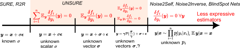
Figure 1: The expressivity-robustness trade-off in self-supervised denoising. If the noise distribution is fully known, SURE provides the most expressive estimator, matching the performance of supervised learning. As the assumptions on the noise are relaxed, the learned estimator needs to be less expressive to avoid over-fitting the noise. In this work, we show that popular ’Noise2x’ strategies impose too restrictive conditions on the learned denoiser, and propose an alternative that strikes a better trade-off.

Noise2Void (Krull et al., 2019), Noise2Self (Batson & Royer, 2019) and similar cross-validation (CV) approaches do not require knowledge about the noise level $\sigma$ by using estimators whose $i$th output $f_{i}(\bm{y})$ does not depend on the $i$th input $y_{i}$, which in turns implies that $\frac{\partial f_{i}}{\partial y_{i}}(\bm{y})=0$ for all pixels $i=1,\dots,n$ and all $\bm{y}\in\mathbb{R}^{m}$. These estimators have thus zero divergence, $\text{div}f(\bm{y})=0$ for all $\bm{y}\in\mathbb{R}^{m}$, and thus can be learned by simply minimizing a data consistency term

$$f^{\text{CV}}=\operatorname*{arg\,min}_{f\in\mathcal{S}_{\text{CV}}}\, \mathbb{E}_{\bm{y}}\,\|f(\bm{y})-\bm{y}\|^{2}$$ (5)

where the function is restricted to the space

$$\mathcal{S}_{\text{CV}}=\{f\in\mathcal{L}^{1}:\frac{\partial f_{i}}{\partial y_{i}}(\bm{y})=0\;\text{for almost every }\bm{y}\in\mathbb{R}^{n}\}.$$

Using the SURE identity in 3, we have the equivalence with the following constrained supervised loss

$$f^{\text{CV}}=\operatorname*{arg\,min}_{f\in\mathcal{S}_{\text{CV}}}\, \mathbb{E}_{\bm{x},\bm{y}}\|f(\bm{y})-\bm{x}\|^{2}$$

whose solution is $f_{i}^{\text{CV}}(\bm{y})=\mathbb{E}\{y_{i}|\bm{y}_{-i}\}=\mathbb{E}\{x_{i}|\bm{y}_{-i}\}$ for $i=1,\dots,n$ where $\bm{y}_{-i}$ denotes $\bm{y}$ excluding the $i$th entry $y_{i}$. The constraint can be enforced in the architecture using convolutional networks whose receptive field does not look at the center pixel (Laine et al., 2019), or via training, by choosing a random set of pixels at each training iteration, setting random values (or the value of one of their neighbors) at the input of the network and computing the loss only at those pixels (Krull et al., 2019).

The zero derivative constraint results in suboptimal estimators, since the $i$th measurement $y_{i}$ generally carries significant information about the value of $x_{i}$. The expected mean squared error of the cross-validation estimator is

$$\mathbb{E}_{\bm{x},\bm{y}}\,\frac{1}{n}\|f^{\text{CV}}(\bm{y})-\bm{x}\|^{2}=\frac{1}{n}\sum_{i=1}^{n}\mathbb{E}_{\bm{y}_{-i}}\,\mathbb{V}\{x_{i}|\bm{y}_{-i}\}$$ (6)

with $\mathbb{V}$ the variance operator, and the performance of this estimator can be arbitrarily bad if there is little correlation between pixels, ie. $\mathbb{V}\{x_{i}|\bm{y}_{-i}\}\approx\mathbb{V}\{x_{i}\}$, in which case the mean squared error is simply the average variance of the ground-truth data $\mathbb{E}_{\bm{x},\bm{y}}\,\frac{1}{n}\|f^{\text{CV}}(\bm{y})-\bm{x}\|^{2}=\frac{1}{n}\sum_{i=1}^{n}\mathbb{V}\{x_{i}\}$.

3 UNSURE

In this work, we propose to relax the zero-derivative constraint of cross-validation, by only requiring that the estimator has zero expected divergence (ZED), ie. $\mathbb{E}_{\bm{y}}\,\text{div}f(\bm{y})=0$. We can blackthen minimize the following problem:

$$f^{\text{ZED}}=\operatorname*{arg\,min}_{f\in\mathcal{S}_{\text{ZED}}}\, \mathbb{E}_{\bm{y}}\|f(\bm{y})-\bm{y}\|^{2}$$ (7)

where $\mathcal{S}_{\text{ZED}}=\{f\in\mathcal{L}^{1}:\mathbb{E}_{\bm{y}}\,\text{div}f(\bm{y})=0\}.$ Since we have that $\mathcal{S}_{\text{CV}}\subset\mathcal{S}_{\text{ZED}}$, blackthe estimator that is divergence-free in expectation is more expressive than the cross-validation counterpart. Again due to SURE, 7 is equivalent to the following constrained supervised loss

$$f^{\text{ZED}}=\operatorname*{arg\,min}_{f\in\mathcal{S}_{\text{ZED}}}\, \mathbb{E}_{\bm{x},\bm{y}}\|f(\bm{y})-\bm{x}\|^{2}$$ (8)

The constrained self-supervised loss in 7 can be formulated using a Lagrange multiplier $\eta\in\mathbb{R}$ as

$$\min_{f}\max_{\eta}\, \mathbb{E}_{\bm{y}}\,\|f(\bm{y})-\bm{y}\|^{2}+2\eta\,\text{div}f(\bm{y})$$ (UNSURE)

which has a simple closed-form solution:

Proposition 1.

The solution of UNSURE is given by

$$f^{\textup{ZED}}{(\bm{y})}=\bm{y}+\hat{\eta}\nabla\log p_{\bm{y}}(\bm{y})$$ (9)

where $\hat{\eta}=(\frac{1}{n}\mathbb{E}_{\bm{y}}\|\nabla\log p_{\bm{y}}(\bm{y})\|^{2})^{-1}\in\mathbb{R}_{+}$ is the optimal multiplier.

A natural question at this point is, how good blackcan a ZED denoiser be? The theoretical performance of an optimal ZED denoiser is provided by the following result:

Proposition 2.

The mean squared error of the optimal divergence-free blackin expectation denoiser is given by

$$\mathbb{E}_{\bm{x},\bm{y}}\,\frac{1}{n}\|f^{\textup{ZED}}{(\bm{y})}-\bm{x}\|^{2}=\sigma^{2}(\frac{1}{1-\frac{\textup{MMSE}}{\sigma^{2}}}-1)$$ (10)

where $\textup{MMSE}=\mathbb{E}_{\bm{x},\bm{y}}\,\frac{1}{n}\|\mathbb{E}\{\bm{x}|\bm{y}\}-\bm{x}\|^{2}$ is the minimum mean squared error.

The proofs of both propositions are included in Appendix A.

We can derive several important observations from these propositions:

1. As with Tweedie’s formula, the optimal divergence-free blackin expectation estimator in 9 can also be interpreted as doing a gradient descent step on $\log p_{\bm{y}}$, but the formula is agnostic to the noise level $\sigma$, as one only requires knowledge of $\nabla\log p_{\bm{y}}(\bm{y})$ to compute the estimator.

2. The step size $\hat{\eta}$ is a conservative estimate of the noise level, as we have that

   $$\hat{\eta}=\frac{\sigma^{2}}{1-\frac{\text{MMSE}}{\sigma^{2}}}\geq\sigma^{2}$$ (11)

3. As we have that $\mathbb{E}_{\bm{y}}\|\nabla\log p_{\bm{y}}(\bm{y})\|^{2}=-\sum_{i}\mathbb{E}_{\bm{y}}\frac{\partial^{2}\log p_{\bm{y}}(\bm{y})}{\partial y_{i}^{2}}$, 9 ressembles the natural gradient descent algorithm (Amari, 2016).

4. Combining 4 and 9, we can write $f^{\text{ZED}}$ as the convex combination of the MMSE estimator and the noisy input:

   $$f^{\textup{ZED}}{(\bm{y})}=\omega\mathbb{E}\{\bm{x}|\bm{y}\}+(1-\omega)\bm{y}$$ (12)

   where $\omega=\frac{n\sigma^{2}}{\mathbb{E}_{\bm{y}}\|\mathbb{E}\{\bm{x}|\bm{y}\}-\bm{y}\|^{2}}\in[0,1]$.

5. We can expand the formula in 10 as a geometric series since $\frac{\text{MMSE}}{\sigma^{2}}<1$ to obtain

   $$\mathbb{E}_{\bm{x},\bm{y}}\,\frac{1}{n}\|f^{\textup{ZED}}{(\bm{y})}-\bm{x}\|^{2}=\text{MMSE}+\sigma^{2}\sum_{j=2}^{\infty}(\frac{\text{MMSE}}{\sigma^{2}})^{j}.$$ (13)

If the support of the signal distribution $p(\bm{x})$ has dimension $k\ll n$, we have that $\text{MMSE}\approx\sigma^{2}k/n$ (Chandrasekaran & Jordan, 2013), and thus i) the estimation of the noise level is accurate as $\hat{\eta}\approx\sigma^{2}+(\frac{\sigma k}{n})^{2}$, and ii) the blackZED estimator performs similarly to the minimum mean squared one, $\mathbb{E}_{\bm{x},\bm{y}}\,\frac{1}{n}\|f^{\textup{ZED}}{(\bm{y})}-\bm{x}\|^{2}\approx\text{MMSE}+(\frac{\sigma k}{n})^{2}$. Perhaps surprisingly, in this case the blackZED estimator is close to optimal without adding any explicit constraints about the low-dimensional nature of $p_{\bm{x}}$.

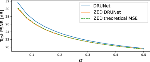
Figure 2: Removing the expected divergence of pretrained MMSE denoisers. Considering the DRUNet as an approximate MMSE denoiser, we use the formula in 12 to evaluate its ZED version and plot the expected theoretical error according to 10. The ZED correction only results in a loss of less than 1 dB for most noise levels. Moreover, the theoretical error follows very closely the empirical one.

The blackZED estimator fails blackwith high-entropy distributions, for example $p_{\bm{x}}=\mathcal{N}(\bm{0},I\sigma_{x}^{2})$. In this case, we have $\hat{\eta}=\sigma^{2}+\sigma_{x}^{2}$, as the noise level estimator cannot tell apart the variance coming from the ground truth distribution $\sigma_{x}^{2}$ from that coming from the noise $\sigma^{2}$, and the blackZED estimator is the trivial guess $f^{\text{ZED}}(\bm{y})=\bm{0}$. Fortunately, this worst-case setting is not encountered in practice as most natural signal distributions are low-dimensional. To illustrate this, we evaluate the performance of a pretrained deep denoiser in comparison with its blackZED version on the DIV2K dataset (see Figure 2). Remarkably, the blackZED denoiser performs very similarly to the original denoiser (less than 1 dB difference across most noise levels), and its error is very well approximated by Proposition 2.

3.1 Examples

To gain some intuition about optimal blackZED estimators and their differences with cross-validation, we consider various popular signal distributions that admit an elementwise decomposition $p_{\bm{x}}(\bm{x})=\prod_{i=1}^{n}q_{x}(x_{i})$ where $q_{x}$ is a one-dimensional probability distribution. Since the noise distribution is also separable, we have that $p_{\bm{y}}(\bm{y})=\prod_{i=1}^{n}q_{y}(y_{i})$ where $q_{y}=q_{x}*\mathcal{N}(0,1)$. All estimators are applied in an element-wise fashion, since there is no correlation between entries, ie. $g(y_{i})=f_{i}(y_{i})$ for all $i=1,\dots,n$, where $g:\mathbb{R}\mapsto\mathbb{R}$ is a one-dimensional function. The cross-validation-based estimator cannot exploit any neighbouring information, and will just return a constant value for all inputs, ie. $g(y_{i})=\mathbb{E}_{y_{i}}\{y_{i}\}$, the observed mean. In contrast, both the MMSE and blackZED estimators use the input $y_{i}$ to improve the estimation. In particular, the optimal blackZED estimator is

$$g(y_{i})=y_{i}+\frac{\nabla\log q_{y}(y_{i})}{\mathbb{E}_{y_{i}}[\nabla\log q_{y}(y_{i})]^{2}}$$

where $q_{y}=q_{\bm{x}}\,*\,\mathcal{N}(0,1)$. Table 1 summarizes the distributions, and Figure 3 shows the estimators for each case. In all cases, we have that the cross-validation estimator is trivial $f^{\text{CV}}(\bm{y})=\bm{0}$ where the mean squared error is simply the signal variance, whereas the blackZED estimator depends on $\bm{y}$, except for the (non-sparse) Gaussian signal distribution. Interestingly, while the MMSE estimator always has non-negative derivatives (Gribonval, 2011), the optimal blackZED estimator can have a negative slope.

	Two Deltas	Gaussian	Spike & Slab
$q_{x}$	$\frac{1}{2}\delta_{-1}+\frac{1}{2}\delta_{1}$	$\mathcal{N}(0,1)$	$\frac{1}{2}\mathcal{N}(0,1)+\frac{1}{2}\delta_{0}$
$q_{y}$	$\frac{1}{2}\mathcal{N}(-1,\sigma^{2})+\frac{1}{2}\mathcal{N}(1,\sigma^{2})$	$\mathcal{N}(0,1+\sigma^{2})$	$\frac{1}{2}\mathcal{N}(0,1+\sigma^{2})+\frac{1}{2}\mathcal{N}(0,\sigma^{2})$
MMSE	0.017	0.059	0.043
MSE CV	0.250	1	0.500
MSE ZED	0.024	1	0.135

Table 1: Examples of popular signal distributions, and the mean squared errors (MSE) for different estimators.

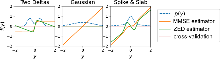
Figure 3: Comparison between MMSE, ZED, and cross-validation estimators for different toy signal distributions.

3.2 Beyond Isotropic Gaussian Noise

Correlated Gaussian noise

In many applications, the noise might be correlated across different pixels. For example, the most popular noise model is

$$\bm{y}|\bm{x}\sim\mathcal{N}(\bm{x},\Sigma)$$

where $\Sigma$ is the covariance matrix capturing the correlations, blackwhich is often partially unknown. This setting is particularly challenging where most self-supervised methods fail. If the noise covariance is known, the SURE formula in is generalized as

$$\mathbb{E}_{\bm{x},\bm{y}}\|f(\bm{y})-\bm{x}\|^{2}=\mathbb{E}_{\bm{y}}\,\left[\|f(\bm{y})-\bm{y}\|^{2}+2\,\textup{tr}\left(\Sigma\frac{\partial f}{\partial\bm{y}}(\bm{y})\right)-n\,\textup{tr}\left(\Sigma\right)\right].$$

blackIf the exact form of the noise covariance is unknown, we can consider an $s$-dimensional set of plausible covariance matrices

$$\mathcal{R}=\{\Sigma_{\bm{\eta}}\in\mathbb{R}^{n\times n}:\Sigma_{\bm{\eta}}=\sum_{j=1}^{s}\eta_{j}\Psi_{j},\bm{\eta}\in\mathbb{R}^{s}\}$$

for some basis matrices $\{\Psi_{j}\in\mathbb{R}^{n\times n}\}_{j=1}^{s}$, with the hope that the true covariance belongs to this set, that is $\Sigma\in\mathcal{R}$. This is equivalent to restricting the learning to estimators in the set $\{f\in\mathcal{L}^{1}:\mathbb{E}_{\bm{y}}\,\,\textup{tr}\left(\Psi_{i}\frac{\partial f}{\partial\bm{y}}(\bm{y})\right)=0,\;i=1,\dots,s\}$. Here, the dimension $s\geq 1$ offers a trade-off between optimality of the resulting estimator and robustness to a misspecified covariance. We can thus generalize UNSURE as

$$\min_{f}\max_{\bm{\eta}}\, \mathbb{E}_{\bm{y}}\,\|f(\bm{y})-\bm{y}\|^{2}+2\,\textup{tr}\left({\Sigma}_{\bm{\eta}}\,f(\bm{y})\right).$$ (14)

blackwith Lagrange multipliers $\bm{\eta}\in\mathbb{R}^{s}$. The following theorem provides the solution for this learning problem:

Theorem 3.

blackLet $p_{\bm{y}}=p_{\bm{x}}*\mathcal{N}(\bm{0},\Sigma)$ and assume that $\{\Psi_{j}\in\mathbb{R}^{n\times n}\}_{j=1}^{s}$ are linearly independent. The optimal solution of problem 14 is given by

$$f(\bm{y})=\bm{y}+{\Sigma}_{\hat{\bm{\eta}}}\,\nabla\log p_{\bm{y}}(\bm{y})$$ (15)

where $\hat{\bm{\eta}}=Q^{-1}\bm{v}$, blackwith $Q_{i,j}=\,\textup{tr}\left(\Psi_{i}\mathbb{E}_{\bm{y}}\left[\nabla\log p_{\bm{y}}(\bm{y})\nabla\log p_{\bm{y}}(\bm{y})^{\top}\right]\Psi_{j}^{\top}\right)$ and $v_{i}=\,\textup{tr}\left(\Psi_{i}\right)$ for $i,j=1,\dots,s$.

The proof is included in Appendix A. blackNote that Proposition 1 is a special case with $s=1$ and $\Psi_{1}=I$.

For example, an interesting family of estimators that are more flexible $f^{\text{CV}}$ and can handle a different unknown noise level per pixel, is obtained by considering the diagonal parameterization $\Sigma_{\bm{\eta}}=\text{diag}(\bm{\eta})$. In this case, we have $\hat{\eta}_{i}=(\mathbb{E}_{\bm{y}}\frac{\partial\log p_{\bm{y}}}{\partial y_{i}}(\bm{y})^{2})^{-1}$ for $i=1,\dots,n$, and thus

$$f_{i}(\bm{y})=y_{i}+(\mathbb{E}_{\bm{y}}\frac{\partial\log p_{\bm{y}}}{\partial y_{i}}(\bm{y})^{2})^{-1}\frac{\partial\log p_{\bm{y}}}{\partial y_{i}}(\bm{y})$$

for $i=1,\dots,n$. The estimator verifies the constraint $\mathbb{E}_{y_{i}}\,\frac{\partial f}{\partial y_{i}}(\bm{y})=0$ for all $i=1,\dots,n$, and thus is still more flexible than cross-validation, as the gradients are zero only in expectation.

Another important family is related to spatially correlated noise, which is generally modeled as

$$\bm{y}=\bm{x}+\bm{\sigma}*\bm{\epsilon}$$

where $*$ denotes the convolution operator, black$\bm{\sigma}\in\mathbb{R}^{p}$ is a vector-valued and $\bm{\epsilon}\sim\mathcal{N}(\bm{0},I)$. blackIf we don’t know the exact noise correlation, we can considering the set of covariances with correlations up to $\pm r$ taps/pixels, we can minimize

$$\min_{f\in\mathcal{S}_{\text{C}}}\mathbb{E}_{\bm{y}}\|f(\bm{y})-\bm{y}\|^{2}$$ (16)

with $\mathcal{S}_{\text{C}}=\{f\in\mathcal{L}^{1}:\mathbb{E}_{\bm{y}}\sum_{i=1}^{n}\frac{\partial f_{i}}{\partial y_{(i+j)\text{ mod }n}}(\bm{y})=0,\;j\in\{-r,\dots,r\}\}$, or equivalently

$$\min_{f}\max_{\bm{\eta}}\, \mathbb{E}_{\bm{y}}\,\|f(\bm{y})-\bm{y}\|^{2}+\sum_{j=-r}^{r}\eta_{j}\,\sum_{i=1}^{n}\frac{\partial f_{i}}{\partial y_{(i+j)\text{ mod }n}}(\bm{y})$$ (C-UNSURE)

whose solution is $f(\bm{y})=\bm{y}+\hat{\bm{\eta}}*\nabla\log p_{\bm{y}}(\bm{y})$ where the optimal multipliers are given by $\hat{\bm{\eta}}=\textcolor{black}{F^{-1}(\bm{1}\bm{/}F\bm{h})}$ where the division is performed elementwise, $\bm{h}\in\mathbb{R}^{2r+1}$ is the $\pm r$ tap autocorrelation of the score and $F\in\mathbb{C}^{(2r+1)\times(2r+1)}$ is the discrete Fourier transform (see Appendix A for more details).

Poisson-Gaussian noise

In many applications, the noise has a multiplicative nature due to the discrete nature of photon-counting detectors. The Poisson-Gaussian noise model is stated as (Le Montagner et al., 2014)

$$\bm{y}=\gamma\mathcal{P}(\frac{\bm{x}}{\gamma})+\sigma\bm{\epsilon}$$ (17)

where $\mathcal{P}$ denotes the Poisson distribution, and the variance of the noise is dependent on the signal level, since $\mathbb{V}\{y_{i}|x_{i}\}=x_{i}\gamma+\sigma^{2}$. In this case, we minimize

$$\min_{f\in\mathcal{S}_{\text{PG}}}\mathbb{E}_{\bm{y}}\,\|f(\bm{y})-\bm{y}\|^{2}$$ (18)

with $\mathcal{S}_{\text{PG}}=\{f\in\mathcal{L}^{1}:\mathbb{E}_{\bm{y}}\,\text{div}f(\bm{y})=0,\;\mathbb{E}_{\bm{y}}\,{\bm{y}}^{\top}\nabla f(\bm{y})=0\}$, or equivalently

$$\min_{f}\max_{\eta,\gamma}\, \mathbb{E}_{\bm{y}}\left[\,\|f(\bm{y})-\bm{y}\|^{2}+\sum_{i=1}^{n}2(\eta+y_{i}\gamma)\,\frac{\partial f_{i}}{\partial y_{i}}(\bm{y})\right]$$ (PG-UNSURE)

whose solution is $f(\bm{y})=\bm{y}+(\bm{1}\hat{\eta}+\bm{y}\hat{\gamma})\circ\nabla\log p_{\bm{y}}(\bm{y})+\bm{1}\hat{\gamma}$ where $\hat{\eta}$ and $\hat{\gamma}$ are included in Appendix C.

Exponential family noise distributions

We can generalize UNSURE to other noise distributions with unknown variance by considering a generalization of Stein’s lemma, introduced by Hudson (1978). In this case, we consider the constrained set $\{f\in\mathcal{L}^{1}:\mathbb{E}_{\bm{y}}\sum_{i=1}^{n}a(y_{i})\frac{\partial f_{i}}{\partial y_{i}}(\bm{y})=0\}$ for some function $a:\mathbb{R}\mapsto\mathbb{R}$ which depends on the noise distribution. For example, the isotropic Gaussian noise case is recovered with $a(y_{i})=1$. See Appendix B for more details.

General inverse problems

We consider problems beyond denoising $\bm{y}=A\bm{x}+\bm{\epsilon}$, where $\bm{y},\bm{\epsilon}\in\mathbb{R}^{m}$, $\bm{x}\in\mathbb{R}^{n}$ and $A\in\mathbb{R}^{m\times n}$ where generally we have fewer measurements than pixels, ie. $m<n$. We can adapt UNSURE to learn in the range space of $A^{\top}$ via

$$\min_{f}\max_{\eta}\,\mathbb{E}_{\bm{y}}\|A^{\dagger}\left(Af(\bm{y})-\bm{y}\right)\|^{2}+2\eta\,\text{div}\left[(A^{\dagger})^{\top}A^{\dagger}Af\right](\bm{y})$$ (General UNSURE)

where $A^{\dagger}\in\mathbb{R}^{n\times m}$ is the linear pseudoinverse of $A$ (Eldar, 2009), or a stable approximation blackthereof. As with SURE, the proposed loss only provides an estimate of the error in the nullspace of $A$. To learn in the nullspace of $A$, we use General UNSURE with the equivariant imaging (EI) loss (Chen et al., 2021), which leverages the invariance of natural image distributions to geometrical transformations (shifts, rotations, etc.), please see Appendix D for more details. A theoretical analysis about learning in incomplete problems can be found in Tachella et al. (2023a).

4 Method

We propose two alternatives for learning the optimal blackZED estimators: the first solves the Lagrange problem in 14, whereas the second one approximates the score during training, and uses the formula in Theorem 3 for inference.

UNSURE

We can solve the optimization problem in 14 by parametrizing the estimator $f_{\bm{\theta}}$ using a deep neural network with weights $\bm{\theta}\in\mathbb{R}^{p}$, and approximating the expectation over $\bm{y}$ by a sum over a dataset of noisy images $\{\bm{y}_{j}\}_{j=1}^{N}$. During training, we search for a saddle point of the loss on $\bm{\theta}$ and $\bm{\eta}$ by alternating between a gradient descent step on $\bm{\theta}$ and a gradient ascent step on $\bm{\eta}$. The gradient with respect to $\bm{\eta}$ does not require additional backpropagation through $f_{\bm{\theta}}$ and thus adds a minimal computational overhead. We approximate the divergence using a Monte Carlo approximation (Ramani et al., 2008)

$$\,\textup{tr}\left(\textcolor{black}{M}\frac{\partial f_{\bm{\theta}}}{\partial\bm{y}}(\bm{y})\right)\approx\frac{(\textcolor{black}{M}\,\bm{b})^{\top}}{\tau}\left(f_{\bm{\theta}}(\bm{y}+\tau\bm{b})-f_{\bm{\theta}}(\bm{y})\right)$$ (19)

where black$M\in\mathbb{R}^{n\times n}$, $\bm{b}\sim\mathcal{N}(0,I)$ and $\tau=0.01$ is a small constant, and for computing the divergence in UNSURE we choose black$M=I$, and for computing the second term in PG-UNSURE we choose black$M=\text{diag}(\eta\bm{1}+\gamma\bm{y})$. A pseudocode for computing the loss is presented in Algorithm 1.

Algorithm 1 UNSURE loss. The standard SURE loss is recovered by setting $\alpha=0$, $\Sigma_{\bm{\eta}}=\Sigma$.

step size $\alpha$, momentum $\mu$, Monte Carlo approximation constant $\tau$

$\text{residual}\leftarrow\|f_{\bm{\theta}}(\bm{y})-\bm{y}\|^{2}$

$\bm{b}\sim\mathcal{N}(\bm{0},I)$

$\text{div}\leftarrow\frac{(\Sigma_{\bm{\eta}}\bm{b})^{\top}}{\tau}\left(f_{\bm{\theta}}(\bm{y}+\tau\bm{b})-f_{\bm{\theta}}(\bm{y})\right)$

$\text{loss}\leftarrow\text{residual}+\text{div}$

$\bm{g}\leftarrow\mu\bm{g}+(1-\mu)\,\frac{\partial\text{div}}{\partial\bm{\eta}}$   # average stochastic gradients w.r.t. $\bm{\eta}$

$\bm{\eta}\leftarrow\bm{\eta}+\alpha\bm{g}$   # gradient ascent Lagrange multipliers

return $\text{loss}(\bm{\theta})$

UNSURE via score

Alternatively, we can approximate the score of the measurement data with a deep network $s_{\theta}(\bm{y})\approx\nabla\log p_{\bm{y}}(\bm{y})$ using the AR-DAE loss proposed in Lim et al. (2020); Kim & Ye (2021),

$$\operatorname*{arg\,min}_{\bm{\theta}}\mathbb{E}_{(\bm{y},\bm{b},\tau)}\,\|\bm{b}+\tau s_{\bm{\theta}}(\bm{y}+\tau\bm{b})\|^{2}$$ (20)

where $\bm{b}\sim\mathcal{N}(\bm{0},I)$ and $\tau\sim\mathcal{N}(\bm{0},\delta^{2})$. Following Lim et al. (2020), we start with a large standard deviation by setting $\delta_{\max}$ and anneal it to a smaller value $\delta_{\min}$ during training. At inference time, we reconstruct the measurements $\bm{y}$ using Theorem 3, as it only requires access to the score:

$$f_{\bm{\theta}}(\bm{y})=\bm{y}+{\Sigma}_{\hat{\bm{\eta}}}\,s_{\bm{\theta}}(\bm{y})$$

where ${\Sigma}_{\hat{\bm{\eta}}}$ is computed using Theorem 3 with $H\approx\mathbb{E}_{\bm{y}}\,{s_{\bm{\theta}}(\bm{y})s_{\bm{\theta}}(\bm{y})^{\top}}$. The expectation can be computed over the whole dataset or a single noisy image if the noise varies across the dataset. As we will see in the following section, this approach requires a single model evaluation per gradient descent step, compared to two evaluations when learning $f_{\bm{\theta}}$ for computing 19, but it requires more epochs to converge and obtained slightly worse reconstruction results in our experiments.

5 Experiments

We show the performance of the proposed loss in various inverse problems and compare it with state-of-the-art self-supervised methods. All our experiments are performed using the deep inverse library (Tachella et al., 2023b). We use the AdamW optimizer for optimizing network weights $\bm{\theta}$ with step size $5\times 10^{-4}$ and default momentum parameters, and set $\alpha=0.01$, $\mu=0.9$ and $\tau=0.01$ for computing the UNSURE loss in Algorithm 1. Examples of reconstructed images are shown in Figure 5.

Gaussian denoising on MNIST

We evaluate the proposed loss for different noise levels $\sigma\in\{0.05,0.1,0.2,0.3,0.4,0.5\}$ of Gaussian noise on the MNIST dataset. We compare with Noise2Score (Kim et al., 2022), Neighbor2Neighbor (Huang et al., 2021), recorrupted2recorrupted (Pang et al., 2021) and SURE (Metzler et al., 2020) and use the same U-Net architecture for all experiments (see Appendix D for more details). The results are shown in Figure 4. The Lagrange multiplier $\eta$ converges in a few epochs to a slightly larger value of $\sigma$ for all evaluated noise levels. SURE and R2R are highly sensitive to the choice of $\sigma$, providing large errors when the noise level is wrongly specified. The proposed UNSURE loss and UNSURE via score do not require knowledge about the noise level and perform only slightly worse than the supervised case. We also evaluate the UNSURE via score approach using image-wise noise level estimations, obtaining a similar performance than averaging over the whole dataset. As the best results are obtained by the UNSURE loss, we use this variant in the rest of our experiments.

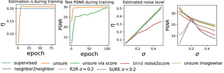
Figure 4: MNIST denoising experiments. From left to right: i) evolution of the Lagrange multiplier $\eta$ for the case with $\sigma=0.2$, ii) test PSNR during training for UNSURE and UNSURE via score with $\sigma=0.1$, iii) estimated Lagrange multiplier as a function of $\sigma$, iv) average test PSNR for various methods and various noise levels $\sigma$.

Colored Gaussian noise on DIV2K

We evaluate the performance of the proposed method on correlated noise on the DIV2K dataset (Zhang et al., 2017), by adding Gaussian noise convolved with a box blur kernel of $3\times 3$ pixels. To capture the spatial structure of noise, we parameterize $\Sigma_{\bm{\eta}}$ in 14 as a circulant (convolution) matrix, as explained in Section 3.2. It is worth noting that only a bound on the support of the blur is needed for the proposed method, while the specific variance in each direction is not necessary. We train all the models on 900 noisy patches of $128\times 128$ pixels extracted from the training set and test on the full validation set which contains images of more than $512\times 512$ pixels.

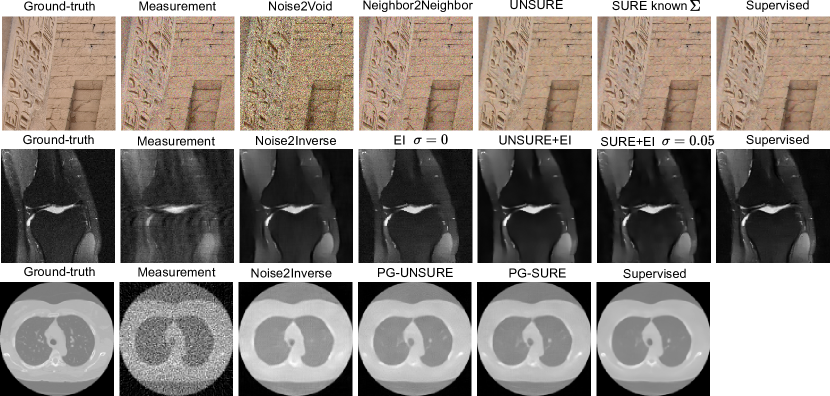
Figure 5: Image reconstruction results for various imaging problems. Top: colored Gaussian noise on DIV2K. Middle: Accelerated magnetic resonance imaging with FastMRI. Bottom: computed tomography with Poisson-Gaussian noise on LIDC

Table 2 shows the test results for the different evaluated methods (Neighbor2Neighbor, Noise2Void and SURE). The proposed method significantly outperforms other self-supervised baselines which fail to capture correlation, performing close ($\approx$ 1 dB) to the SURE method with known noise covariance and supervised learning. Table 3 shows the impact of the choice of the kernel size in the proposed method, where overspecifying the kernel size provides a significant improvement over underspecification, and a mild performance reduction compared to choosing the exact kernel size.

Method	Noise2Void	Neighbor2Neighbor	UNSURE (unknown $\Sigma$)	SURE (known $\Sigma$)	Supervised
PSNR [dB]	$19.09\pm 1.79$	$23.61\pm 0.13$	$28.72\pm 1.03$	$29.77\pm 1.22$	$29.91\pm 1.26$

Table 2: Average test PSNR of learning methods for correlated Gaussian noise.

Kernel size $\bm{\eta}$	$1\times 1$	$3\times 3$	$5\times 5$
PSNR [dB]	23.62	$28.72\pm 1.03$	$27.38\pm 0.88$

Table 3: Average test PSNR of the proposed method as a function of the chosen blur kernel size, where the ground-truth kernel had size $3\times 3$.

Computed tomography with Poisson-Gaussian noise on LIDC

We evaluate a tomography problem where (resized) images of $128\times 128$ pixels taken from the LIDC dataset, are measured using a parallel beam tomography operator with $128$ equispaced angles (thus $A$ does not have a significant nullspace). The measurements are corrupted by Poisson-Gaussian noise distribution in 17 of levels $\gamma=\sigma=0.005$. We compare our method with the Poisson-Gaussian SURE loss proposed in (Le Montagner et al., 2014), and a cross-validation approach blacksimilar to Noise2Inverse (Hendriksen et al., 2020). In this case, we use the loss in PG-UNSURE with $\eta$ and $\gamma$ as Lagrange multipliers, together with the pseudoinverse correction in General UNSURE. We evaluate all methods using an unrolled network with a U-Net denoiser backbone (see Appendix D for details). Table 4 presents the test PSNR of the compared methods. The proposed loss outperforms the cross-validation approach while being close to SURE with known noise levels.

Method	Noise2Inverse	PG-UNSURE (unknown $\sigma,\,\gamma$)	PG-SURE (known $\sigma,\,\gamma$)	Supervised
PSNR [dB]	$32.54\pm 0.71$	$33.31\pm 0.57$	$33.76\pm 0.61$	$34.67\pm 0.68$

Table 4: Average test PSNR of learning methods for computed tomography with Poisson-Gaussian noise.

Accelerated magnetic resonance imaging with FastMRI

We evaluate a single-coil $2\times$-accelerated MRI problem using a subset of 900 images of the FastMRI dataset for training and 100 for testing (Chen et al., 2021), and adding Gaussian noise with $\sigma=0.03$ to the k-space measurements. We evaluate all methods using an unrolled network with a U-Net denoiser backbone (see appendix for more details). We compare with cross-validation, simple measurement consistency ($\|f(\bm{y})-\bm{y}\|^{2}$) and SURE with slightly wrong noise level $\sigma=0.05$. The cross-validation method is equivalent to the SSDU method (Yaman et al., 2020). We add the EI loss with rotations as proposed in (Chen et al., 2021) to all methods since this problem has non-trivial nullspace. Table 5 shows the test PSNR for the compared methods. The proposed method performs better than all other self-supervised methods, and around 1 dB worse than supervised learning.

Method	CV + EI	EI (assumes $\sigma=0$)	UNSURE + EI (unknown $\sigma$)	SURE + EI (assumes $\sigma=0.05$)	Supervised
PSNR [dB]	$33.25\pm 1.14$	$34.32\pm 0.91$	$35.73\pm 1.45$	$28.05\pm 4.73$	$36.63\pm 1.38$

Table 5: Average test PSNR of learning methods for accelerated MRI with noise level $\sigma=0.03$.

6 Limitations

The analysis in this paper is restricted to the $\ell_{2}$ loss, which is linked to minimum squared error distortion. In certain applications, more perceptual reconstructions might be desired (Blau & Michaeli, 2018), and we do not address this goal here. Both SURE and the proposed UNSURE method require an additional evaluation of the estimator during training than supervised learning, and thus the training is more computationally intensive than supervised learning.

7 Conclusion

We present a new framework to understand the robustness-expressivity trade-off of self-supervised learning methods, which characterizes different families of estimators according to the constraints in their (expected) derivatives. This blackanalysis results in a new family of estimators which we call UNSURE, which do not require prior knowledge about the noise level, but that are more expressive than cross-validation methods.

Acknowledgments

Julián Tachella is supported by the ANR grant UNLIP (ANR-23-CE23-0013). Laurent Jacques thanks the FRS-FNRS for the funding related to the PDR project QuadSense (T.0160.24)

Appendix A Proofs

We start by proving Theorem 3, as Propositions 1 and 2 can be then derived as simple corollaries.

Proof.

We want to find the solution of the max-min problem

$$\min_{f}\max_{\bm{\eta}}\;\mathbb{E}_{\bm{y}}\,\left[\|f(\bm{y})-\bm{y}\|^{2}+2\,\,\textup{tr}\left(\Sigma_{\bm{\eta}}\,\frac{\partial f}{\partial\bm{y}}(\bm{y})\right)\right]$$

blackSince the problem is convex with respect to $f$ and has an affine equality constraint, it verifies strong duality (Luenberger, 1969, Chapter 8), and thus we can rewrite it as a max-min problem, that is

$$\max_{\bm{\eta}}\min_{f}\;\mathbb{E}_{\bm{y}}\,\left[\|f(\bm{y})-\bm{y}\|^{2}+2\,\,\textup{tr}\left(\Sigma_{\bm{\eta}}\,\frac{\partial f}{\partial\bm{y}}(\bm{y})\right)\right].$$

Choosing $f(\bm{y})=\bm{y}+\tilde{f}(\bm{y})$, we can rewrite the problem as

$$\max_{\bm{\eta}}\min_{\tilde{f}}\;\mathbb{E}_{\bm{y}}\,\|\tilde{f}(\bm{y})\|^{2}+2\,\textup{tr}\left(\Sigma_{\bm{\eta}}\,\frac{\partial\tilde{f}}{\partial\bm{y}}(\bm{y})\right)+2\,\textup{tr}\left(\Sigma_{\bm{\eta}}\right).$$ (21)

Using integration by parts and the facts that blacki) $p_{\bm{y}}=p_{\bm{x}}*\mathcal{N}(0,\Sigma)$ is differentiable and supported on $\mathbb{R}^{n}$, and ii) $\frac{\partial p_{\bm{y}}}{\partial y_{i}}/p_{\bm{y}}=\frac{\partial\log p_{\bm{y}}}{\partial y_{i}}$, we have that

$$\mathbb{E}_{\bm{y}}\,\frac{\partial\tilde{f}_{i}(\bm{y})}{\partial y_{j}} =\int p_{\bm{y}}(\bm{y})\frac{\partial\tilde{f}_{i}}{\partial y_{j}}(\bm{y})\,d\bm{y}$$ (22)

$$=-\int\tilde{f}_{i}(\bm{y})\frac{\partial p_{\bm{y}}}{\partial y_{j}}(\bm{y})\,d\bm{y}$$ (23)

$$=-\int\tilde{f}_{i}(\bm{y})\frac{\frac{\partial p_{\bm{y}}}{\partial y_{j}}(\bm{y})}{p_{\bm{y}}(\bm{y})}p_{\bm{y}}(\bm{y})\,d\bm{y}$$ (24)

$$=-\mathbb{E}_{\bm{y}}\,\tilde{f}_{i}(\bm{y})\frac{\partial\log p_{\bm{y}}}{\partial y_{j}}(\bm{y}).$$ (25)

and thus $\mathbb{E}_{\bm{y}}\frac{\partial\tilde{f}}{\partial\bm{y}}(\bm{y})=\mathbb{E}_{\bm{y}}\tilde{f}(\bm{y})\nabla\log p_{\bm{y}}(\bm{y})^{\top}$. Plugging this result into 21, we obtain

$$\max_{\bm{\eta}}\min_{\tilde{f}_{1},\dots,\tilde{f}_{n}}\;\mathbb{E}_{\bm{y}}\,\left[\|\tilde{f}(\bm{y})\|^{2}-2\,\textup{tr}\left(\Sigma_{\bm{\eta}}\,\tilde{f}(\bm{y})\nabla\log p_{\bm{y}}(\bm{y})^{\top}\right)\right]+2\,\textup{tr}\left(\Sigma_{\bm{\eta}}\right)$$ (26)

$$\max_{\bm{\eta}}\min_{\tilde{f}_{1},\dots,\tilde{f}_{n}}\;\mathbb{E}_{\bm{y}}\,\left[\|\tilde{f}(\bm{y})\|^{2}-2\tilde{f}(\bm{y})^{\top}\Sigma_{\bm{\eta}}^{\top}\nabla\log p_{\bm{y}}(\bm{y})\right]+2\,\textup{tr}\left(\Sigma_{\bm{\eta}}\right)$$ (27)

where the first term can be rewritten in a quadratic form as

$$\max_{\bm{\eta}}\min_{\tilde{f}}\mathbb{E}_{\bm{y}}\,\|\tilde{f}(\bm{y})-\Sigma_{\bm{\eta}}\nabla\log p_{\bm{y}}(\bm{y})\|^{2}-\,\textup{tr}\left(\Sigma_{\bm{\eta}}H\Sigma_{{\bm{\eta}}}^{\top}\right)+2\,\textup{tr}\left(\Sigma_{\bm{\eta}}\right)$$ (28)

with $H=\mathbb{E}_{\bm{y}}\,\nabla\log p_{\bm{y}}(\bm{y})\nabla\log p_{\bm{y}}(\bm{y})^{\top}$. Since the density $p_{\bm{y}}(\bm{y})>0$ for all $\bm{y}\in\mathbb{R}^{n}$ black(as it is the convolution of $p_{\bm{x}}$ with a Gaussian density), blackthe minimum of 28 with respect to $\tilde{f}$ is

$$\tilde{f}(\bm{y})=\Sigma_{\bm{\eta}}\nabla\log p_{\bm{y}}(\bm{y}).$$ (29)

Replacing this solution in 28, we get

$$\max_{\bm{\eta}}-\,\textup{tr}\left(\Sigma_{{\bm{\eta}}}H\Sigma_{\bm{\eta}}^{\top}\right)+2\,\textup{tr}\left(\Sigma_{\bm{\eta}}\right)$$

which can be rewritten as

$$\min_{\bm{\eta}}\,\textup{tr}\left(\Sigma_{{\bm{\eta}}}H\Sigma_{\bm{\eta}}^{\top}\right)-2\,\textup{tr}\left(\Sigma_{\bm{\eta}}\right)$$ (30)

In particular, if we have $\Sigma_{\bm{\eta}}=\sum_{j=0}^{s}\eta_{j}\Psi_{j}$ for some matrices $\{\Psi_{j}\in\mathbb{R}^{n\times n}\}_{j=1}^{s}$, then the problem simplifies to

$$\min_{\bm{\eta}}\sum_{i,j}\eta_{i}\eta_{j}\,\textup{tr}\left(\Psi_{i}H\Psi_{j}^{\top}\right)-2\eta_{i}\,\textup{tr}\left(\Psi_{i}\right).$$

Setting the gradient with respect to $\bm{\eta}$ to zero results in the quadratic problem $Q\hat{\bm{\eta}}=\bm{v}$ where $Q_{i,j}:=\,\textup{tr}\left(\Psi_{i}H\Psi_{j}^{\top}\right)$ and $v_{i}:=\,\textup{tr}\left(\Psi_{i}\right)$ for $i,j=1,\dots,s$. blackThe matrix $Q$ can be seen as Gram matrix since its entries can be written as inner products $\langle\Psi_{i},\Psi_{j}\rangle_{H}$ where $H$ is positive definite due to the assumption that $p_{\bm{y}}=p_{\bm{x}}*\mathcal{N}(\bm{0},\Sigma)$. Thus, since by assumption the set $\{\Psi_{j}\}_{j=1}^{s}$ is linearly independent, $Q$ is invertible and the optimal $\hat{\bm{\eta}}$ is given by

$$\hat{\bm{\eta}}=Q^{-1}\bm{v}.$$ (31)

∎

We now analyze the mean squared error of blackZED estimators: We can replace the solution $f(\bm{y})=\bm{y}+\Sigma_{\bm{\eta}}\nabla\log p_{\bm{y}}(\bm{y})$ in SURE’s formula to obtain

$$\mathbb{E}_{\bm{x},\bm{y}}\|f(\bm{y})-\bm{x}\|^{2}=\mathbb{E}_{\bm{y}}\|\Sigma_{\bm{\eta}}\nabla\log p_{\bm{y}}(\bm{y})\|^{2}+2\,\textup{tr}\left(\Sigma(I+\Sigma_{\bm{\eta}}\frac{\partial^{2}\log p_{\bm{y}}}{\partial\bm{y}^{2}}(\bm{y}))\right)-\,\textup{tr}\left(\Sigma\right)$$

which can be written as

$$\mathbb{E}_{\bm{x},\bm{y}}\|f(\bm{y})-\bm{x}\|^{2}=\,\textup{tr}\left(\Sigma_{\bm{\eta}}\Sigma_{\bm{\eta}}^{\top}\mathbb{E}_{\bm{y}}\nabla\log p_{\bm{y}}(\bm{y})\nabla\log p_{\bm{y}}(\bm{y})^{\top}\right)+2\,\textup{tr}\left(\Sigma(I+\Sigma_{\bm{\eta}}\frac{\partial^{2}\log p_{\bm{y}}}{\partial\bm{y}^{2}})\right)-\,\textup{tr}\left(\Sigma\right)$$

Using the fact that $\mathbb{E}_{\bm{y}}\,\frac{\partial^{2}\log p_{\bm{y}}}{\partial\bm{y}^{2}}(\bm{y})=-\mathbb{E}_{\bm{y}}\,\nabla\log p_{\bm{y}}(\bm{y})\nabla\log p_{\bm{y}}(\bm{y})^{\top}=-H$, we have

$$\mathbb{E}_{\bm{x},\bm{y}}\|f(\bm{y})-\bm{x}\|^{2}=\,\textup{tr}\left(\Sigma_{\bm{\eta}}\Sigma_{\bm{\eta}}^{\top}H\right)-2\,\textup{tr}\left(\Sigma\Sigma_{\bm{\eta}}H\right)+\,\textup{tr}\left(\Sigma\right)$$

Proof of Propositions 1 and 2:

Proof.

In this case, we have $\Sigma_{\eta}=\eta I$, and thus 31 reduces to

$$\hat{\eta}=\frac{\,\textup{tr}\left(I\right)}{\,\textup{tr}\left(H\right)}=\frac{n}{\mathbb{E}_{\bm{y}}\|\nabla\log p_{\bm{y}}(\bm{y})\|^{2}}$$ (32)

and the mean squared error is given by

$$\mathbb{E}_{\bm{x},\bm{y}}\|f(\bm{y})-\bm{x}\|^{2}=\hat{\eta}-\sigma^{2}$$

which can be rewritten as

$$\hat{\eta}=\mathbb{E}_{\bm{x},\bm{y}}\|f(\bm{y})-\bm{x}\|^{2}+\sigma^{2}$$ (33)

Noting that $\text{MMSE}=\sigma^{2}-\sigma^{4}\frac{1}{n}\mathbb{E}_{\bm{y}}\|\nabla\log p_{\bm{y}}(\bm{y})\|^{2}=\sigma^{2}-\frac{\sigma^{4}}{\hat{\eta}}$, we have that

$$\hat{\eta}=\frac{\sigma^{4}}{\sigma^{2}-\text{MMSE}}$$ (34)

Combining 33 and 12, we have

$$\mathbb{E}_{\bm{x},\bm{y}}\|f(\bm{y})-\bm{x}\|^{2} =\frac{\sigma^{4}}{\sigma^{2}-\text{MMSE}}-\sigma^{2}$$ (35)

$$=\sigma^{2}(\frac{1}{1-\frac{\text{MMSE}}{\sigma^{2}}}-1).$$ (36)

∎

Anisotropic noise

In this case, we have $\Sigma_{\eta}=\text{diag}(\bm{\eta})=\sum_{j=1}^{n}\eta_{j}\bm{e}_{j}\bm{e}_{j}^{\top}$, and thus we have $Q=\text{diag}(H)$ and $\bm{v}=n\bm{1}$ in 31, giving the solution

$$\hat{\eta}_{i}=\frac{1}{\frac{1}{n}\mathbb{E}_{\bm{y}}[\frac{\partial\log p_{\bm{y}}}{\partial y_{i}}(\bm{y})]^{2}}$$ (37)

for $i=1,\dots,n$.

Correlated noise

If we consider the 1D setting, we have $\Sigma_{\eta}=\text{circ}(\bm{\eta})=\sum_{j=1}^{2r+1}\eta_{j}T_{j-r}$ blackis a circulant matrix, where $T_{j}$ is the $j$-tap shift matrix, and thus $\bm{v}=n\,\textcolor{black}{\bm{e}_{r+1}}$ and $Q=n\,\text{circ}(\bm{h})$ where $\bm{h}\in\mathbb{R}^{2r+1}$ is the autocorrelation of $\nabla\log p_{\bm{y}}(\bm{y})$ (considering up to $\pm j$ taps) , that is

$$h_{j}=\frac{1}{n}\sum_{i=1}^{n}\mathbb{E}_{\bm{y}}\frac{\partial\log p_{\bm{y}}}{\partial y_{i}}\frac{\partial\log p_{\bm{y}}}{\partial y_{(i+j-r)\text{ mod }n}}(\bm{y})$$

for $j=1,\dots,2r+1$, blackand $\bm{e}_{r+1}$ denotes the $(r+1)$th canonical vector. Thus, we have $\hat{\bm{\eta}}=\text{circ}(\bm{h})^{-1}\textcolor{black}{\bm{e}_{r+1}}$, or equivalently

$$\hat{\bm{\eta}}=\textcolor{black}{F^{-1}(\bm{1}\bm{/}F\bm{h})}$$

where the division is performed elementwise and $F\in\mathbb{C}^{(2r+1)\times(2r+1)}$ is the discrete Fourier transform.

Appendix B Exponential family

We now consider separable noise distributions $p(\bm{y}|\bm{x})=\prod_{i=1}^{n}q(y_{i}|x_{i})$, where $q(x|y)$ belongs to the exponential family

$$q(y|x)=h(y)\exp(r(x)b(y)-\psi(x))$$

where $\psi(x)=\log\int h(y)\exp(r(x)b(y))$ is the normalization function.

Lemma 4.

Let $\bm{y}\sim p(\bm{y}|\bm{x})=\prod_{i=1}^{n}q(y_{i}|x_{i})$ be a random variable with mean $\mathbb{E}_{\bm{y}|\bm{x}}\bm{y}=\bm{x}$, where the distribution $q$ belongs to the set $\mathcal{C}$ whose definition is included in Appendix A. Then,

$$\mathbb{E}_{\bm{y}|\bm{x}}(\bm{y}-\bm{x})^{\top}f(\bm{y})=\sigma^{2}\sum_{i=1}^{n}\mathbb{E}_{\bm{y}|\bm{x}}a(y_{i})\frac{\partial f_{i}}{\partial y_{i}}(\bm{y})$$ (38)

where $a:\mathbb{R}\mapsto[0,\infty)$ is a non-negative scalar function and $\sigma^{2}=\frac{1}{n}\mathbb{E}_{\bm{y}|\bm{x}}\|\bm{y}-\bm{x}\|^{2}$ is the noise variance.

Stein’s lemma can be seen as a special case of Lemma 4 by setting $a(y)=1$, which corresponds to the case of Gaussian noise. If the noise variance $\sigma^{2}$ is unknown, we can minimize

$$\min_{f\in\mathcal{S}_{\text{H}}}\,\mathbb{E}_{\bm{y}}\,\|f(\bm{y})-\bm{y}\|^{2}$$ (39)

where $\mathcal{S}_{\text{H}}=\{f\in\mathcal{L}^{1}:\sum_{i=1}^{n}\mathbb{E}_{\bm{y}}a(y_{i})\frac{\partial f_{i}}{\partial y_{i}}(\bm{y})=0\}$. Again, we consider the Lagrange formulation of the problem:

$$\max_{\eta}\min_{f}\, \mathbb{E}_{\bm{y}}\left[\,\|f(\bm{y})-\bm{y}\|^{2}+2\eta\sum_{i=1}^{n}\,a(y_{i})\frac{\partial f_{i}}{\partial y_{i}}(\bm{y})\right]$$ (40)

where we only need to know $a(\cdot)$ up to a proportionality constant. The solution to this problem is given by

$$f(\bm{y})=\bm{y}+\hat{\eta}\left(a(\bm{y})\circ\nabla\log p_{\bm{y}}(\bm{y})+\nabla a(\bm{y})\right).$$

where $\hat{\eta}$ is also available in closed form (see Appendix A for details). Note that when $a(y)=1$, 40 boils down to the isotropic Gaussian noise case UNSURE.

Lemma 4 (Hudson, 1978) applies to a subset $\mathcal{C}$ of the exponential family where $r(x)=x$, $h(y)=\frac{\partial b}{\partial y}(y)\exp(b(y)y-\int b(u)du)$ and $\frac{\partial b}{\partial y}(y)=1/a(y)$, with $\int b(u)du$ interpreted as an indefinite integral. In this case, we aim to minimize the following problem:

$$\max_{\eta}\min_{f}\mathbb{E}_{\bm{y}}\|\bm{y}-f(\bm{y})\|^{2}+2\eta\sum_{i=1}^{n}a(y_{i})\frac{\partial f_{i}}{\partial y_{i}}(\bm{y})$$ (41)

for some non-negative function $a:\mathbb{R}\mapsto[0,\infty)$. As with the Gaussian case, we can look for a solution $f(\bm{y})=\bm{y}+\tilde{f}(\bm{y})$, that is

$$\max_{\eta}\min_{\tilde{f}}\mathbb{E}_{\bm{y}}\|\tilde{f}(\bm{y})\|^{2}+2\eta\sum_{i=1}^{n}\left(a(y_{i})+a(y_{i})\frac{\partial\tilde{f}_{i}}{\partial y_{i}}(\bm{y})\right)$$ (42)

and follow the same steps, using the following generalization of 22:

$$\mathbb{E}_{\bm{y}}\,a(y_{i})\frac{\partial\tilde{f}_{i}(\bm{y})}{\partial y_{i}} =\int p_{\bm{y}}(\bm{y})a(y_{i})\frac{\partial\tilde{f}_{i}}{\partial y_{i}}(\bm{y})\,d\bm{y}$$ (43)

$$=-\int\tilde{f}_{i}(\bm{y})[a(y_{i})\frac{\partial p_{\bm{y}}}{\partial y_{i}}(\bm{y})+\frac{\partial a}{\partial y_{i}}(y_{i})p_{\bm{y}}(\bm{y})]\,d\bm{y}$$ (44)

$$=-\int\tilde{f}_{i}(\bm{y})[a(y_{i})\frac{\frac{\partial p_{\bm{y}}}{\partial y_{j}}(\bm{y})}{p_{\bm{y}}(\bm{y})}+\frac{\partial a}{\partial y_{i}}(y_{i})]p_{\bm{y}}(\bm{y})\,d\bm{y}$$ (45)

$$=-\mathbb{E}_{\bm{y}}\,\tilde{f}_{i}(\bm{y})[a(y_{i})\frac{\partial\log p_{\bm{y}}}{\partial y_{j}}(\bm{y})+\frac{\partial a}{\partial y_{i}}(y_{i})]$$ (46)

to obtain the solution $\tilde{f}(\bm{y})=\eta s(\bm{y})$ with $s(\bm{y})=a(\bm{y})\circ\nabla\log p_{\bm{y}}(\bm{y})+\nabla a(\bm{y})$. Replacing the optimal $\tilde{f}$ in 41, we have the following problem for $\eta$:

$$\max_{\eta}\eta^{2}\mathbb{E}_{\bm{y}}\|s(\bm{y})\|^{2}+2\eta\sum_{i=1}^{n}\mathbb{E}_{y_{i}}a(y_{i})+2\eta^{2}\sum_{i=1}^{n}\mathbb{E}_{\bm{y}}a(y_{i})\frac{\partial s_{i}}{\partial y_{i}}(\bm{y})$$ (47)

which is a quadratic problem whose solution is

$$\hat{\eta}=\frac{\sum_{i=1}^{n}\mathbb{E}_{y_{i}}a(y_{i})}{\sum_{i=1}^{n}-\mathbb{E}_{\bm{y}}s_{i}(\bm{y})^{2}-2\mathbb{E}_{\bm{y}}a(y_{i})\frac{\partial s_{i}}{\partial y_{i}}(\bm{y})}$$ (48)

Thus, the minimizer of 41 is

$$f(\bm{y})=\bm{y}+\hat{\eta}\left(a(\bm{y})\circ\nabla\log p_{\bm{y}}(\bm{y})+\nabla a(\bm{y})\right).$$

Appendix C Poisson-Gaussian noise

The PG-SURE estimator for the Poisson-Gaussian noise model in 17 is given by (Le Montagner et al., 2014)

$$\mathbb{E}_{\bm{y}}\left[\,\|f(\bm{y})\|^{2}+\|\bm{y}\|^{2}+\sum_{i=1}^{n}2\sigma^{2}\,\frac{\partial f_{i}}{\partial y_{i}}(\bm{y}-\bm{e}_{i}\gamma)-2y_{i}f_{i}(\bm{y}-\bm{e}_{i}\gamma)-\gamma y_{i}\right]-\sigma^{2}$$ (49)

where $\bm{e}_{i}$ denotes the $i$th canonical vector. Following Le Montagner et al. (2014), we use the approximation

$$f_{i}(\bm{y}-\bm{e}_{i}\gamma)\approx f_{i}(\bm{y})-\gamma\frac{\partial f_{i}}{\partial y_{i}}(\bm{y})$$

and

$$\frac{\partial f_{i}}{\partial y_{i}}(\bm{y}-\bm{e}_{i}\gamma)\approx\frac{\partial f_{i}}{\partial y_{i}}(\bm{y})-\gamma\frac{\partial^{2}f_{i}}{\partial{y_{i}}^{2}}(\bm{y})$$

to obtain

$$\mathbb{E}_{\bm{y}}\left[\,\|f(\bm{y})-\bm{y}\|^{2}+\sum_{i=1}^{n}(2\sigma^{2}+2y_{i}\gamma)\,\frac{\partial f_{i}}{\partial y_{i}}(\bm{y})+2\sigma^{2}\gamma\frac{\partial^{2}f_{i}}{\partial{y_{i}}^{2}}(\bm{y})-\gamma y_{i}\right]-\sigma^{2}$$ (50)

We can obtain the PG-UNSURE estimator by replacing $(\gamma,\sigma^{2})$ for the Lagrange multipliers $(\gamma,\sigma)$ to obtain

$$\max_{\eta,\gamma}\min_{f}\mathbb{E}_{\bm{y}}\left[\,\|f(\bm{y})-\bm{y}\|^{2}+\sum_{i=1}^{n}(2\eta+2y_{i}\gamma)\,\frac{\partial f_{i}}{\partial y_{i}}(\bm{y})\right]$$ (51)

where we drop the second order derivative, since we observe that in practice we have $|\frac{\partial^{2}f_{i}}{\partial{y_{i}}^{2}}(\bm{y})|\ll|\frac{\partial f_{i}}{\partial y_{i}}(\bm{y})|$. Note that this problem is equivalent to

$$\operatorname*{arg\,min}_{f\in\mathcal{S}_{\text{PG}}}\max_{\eta,\gamma}\mathbb{E}_{\bm{y}}\,\|f(\bm{y})-\bm{y}\|^{2}$$ (52)

where $\mathcal{S}_{\text{PG}}=\{f:\mathbb{E}_{\bm{y}}\text{div}f(\bm{y})=0,\;\mathbb{E}_{\bm{y}}{\bm{y}}^{\top}\nabla f(\bm{y})=0\}$ and thus we have that $\mathcal{S}_{\text{CV}}\subset\mathcal{S}_{\text{PG}}\subset\mathcal{S}_{\text{ZED}}$.

Setting $f(\bm{y})=\bm{y}+\tilde{f}(\bm{y})$, we can rewrite problem 51 as

$$\max_{\eta,\gamma}\operatorname*{arg\,min}_{f}\sum_{i=1}^{n}\mathbb{E}_{\bm{y}}\,\tilde{f}_{i}(\bm{y})^{2}+(2\eta+2y_{i}\gamma)\,\frac{\partial\tilde{f}_{i}}{\partial y_{i}}(\bm{y})+2\eta+2\gamma y_{i}$$ (53)

Using integration by parts as in 22, we get

$$\max_{\eta,\gamma}\operatorname*{arg\,min}_{f}\sum_{i=1}^{n}\mathbb{E}_{\bm{y}}\,\tilde{f}_{i}(\bm{y})^{2}-2\tilde{f}_{i}(\bm{y})\left((\eta+y_{i}\gamma)\frac{\partial\log p_{\bm{y}}}{\partial y_{i}}(\bm{y})+\gamma\right)^{2}\,+2\eta+2\gamma y_{i}$$

After completing squares, we obtain

$$\max_{\eta,\gamma}\operatorname*{arg\,min}_{f}\sum_{i=1}^{n}\mathbb{E}_{\bm{y}}\left(\tilde{f}_{i}(\bm{y})-(\eta+y_{i}\gamma)\frac{\partial\log p_{\bm{y}}}{\partial y_{i}}(\bm{y})-\gamma\right)^{2}-\left((\eta+y_{i}\gamma)\frac{\partial\log p_{\bm{y}}}{\partial y_{i}}(\bm{y})-\gamma\right)^{2}+2\eta+2\gamma y_{i}$$

thus we have

$$\tilde{f}(\bm{y})=(\bm{1}\eta+\bm{y}\gamma)\circ\nabla\log p_{\bm{y}}(\bm{y})+\bm{1}\gamma$$

and

$$f(\bm{y})=\bm{y}+(\bm{1}\eta+\bm{y}\gamma)\circ\nabla\log p_{\bm{y}}(\bm{y})+\bm{1}\gamma$$

where $(\eta,\gamma)$ are given by

$$\max_{\eta,\gamma}\sum_{i=1}^{n}\mathbb{E}_{\bm{y}}-\left(\eta\frac{\partial\log p_{\bm{y}}}{\partial y_{i}}(\bm{y})+y_{i}\gamma\frac{\partial\log p_{\bm{y}}}{\partial y_{i}}(\bm{y})-\gamma\right)^{2}+2\eta+2\gamma y_{i}.$$

Defining the expectations $h_{a,b}:=\sum_{i=1}^{n}\mathbb{E}_{\bm{y}}y_{i}^{a}\frac{\partial\log p_{\bm{y}}}{\partial y_{i}}(\bm{y})^{b}$ for $a,b\in\{0,1,2\}$, we have

$$\max_{\eta,\gamma}-\eta^{2}h_{0,2}-\gamma^{2}h_{2,2}-n\gamma^{2}-2\gamma\eta h_{1,2}+2\eta\gamma h_{0,1}+2\gamma^{2}h_{1,1}+2n\eta+2\gamma h_{1,0}.$$

We can take derivatives with respect to $(\eta,\gamma)$ to obtain the optimality conditions

$$\begin{cases}0&=-\eta h_{0,2}-\gamma h_{1,2}+\gamma h_{0,1}+n\\ 0&=-\gamma h_{2,2}-n\gamma-\eta h_{1,2}+\eta h_{0,1}+2\gamma h_{1,1}+h_{1,0}\end{cases}$$ (54)

which are equivalent to

$$\begin{cases}n&=\eta h_{0,2}+\gamma(h_{1,2}-h_{0,1})\\ h_{1,0}&=\eta(h_{1,2}-h_{0,1})+\gamma(h_{2,2}+n+h_{1,2}-2h_{1,1})\end{cases}.$$ (55)

The solution to this system of equations is

$$\eta=\frac{n}{h_{0,2}}-\frac{\gamma(h_{1,2}-h_{0,1})}{h_{0,2}}$$ (56)

where

$$\gamma=\frac{h_{1,0}h_{0,2}-n(h_{1,2}-h_{0,1})}{h_{0,2}(h_{2,2}+n-2h_{1,1})-(h_{1,2}-h_{0,1})^{2}}.$$ (57)

In particular, if we remove the $\gamma$-constraint ($\gamma=0$), we obtain the UNSURE formula in Proposition 1, ie. $\eta=\frac{n}{h_{0,2}}=(\frac{1}{n}\mathbb{E}_{\bm{y}}\|\nabla\log p_{\bm{y}}(\bm{y})\|^{2})^{-1}$.

Appendix D Experimental Details

We use the U-Net architecture of the deep inverse library (Tachella et al., 2023b) with no biases and an overall skip-connection as a backbone network in all our experiments, only varying the number of scales of the network across experiments.

MNIST denoising

We use the U-Net architecture with 3 scales.

DIV2K denoising

We use the U-Net architecture with 4 scales.

Computed Tomography on LIDC

We use an unrolled proximal gradient algorithm with 4 iterations and no weight-tying across iterations. The denoiser is set as the U-Net architecture with 2 scales.

Accelerated MRI on FastMRI

We use an unrolled half-quadratic splitting algorithm with 7 iterations and no weight-tying across iterations. The denoiser is set as the U-Net architecture with 2 scales.

References

- Aggarwal et al. (2023) Hemant Kumar Aggarwal, Aniket Pramanik, Maneesh John, and Mathews Jacob. ENSURE: A General Approach for Unsupervised Training of Deep Image Reconstruction Algorithms. IEEE Transactions on Medical Imaging, 42(4):1133–1144, April 2023. ISSN 0278-0062, 1558-254X. doi: 10.1109/TMI.2022.3224359. URL http://arxiv.org/abs/2010.10631. arXiv:2010.10631 [cs, eess, stat].
- Almeida & Figueiredo (2013) Mariana S. C. Almeida and Mário A. T. Figueiredo. Parameter Estimation for Blind and Non-Blind Deblurring Using Residual Whiteness Measures. IEEE Transactions on Image Processing, 22(7):2751–2763, July 2013. ISSN 1941-0042. doi: 10.1109/TIP.2013.2257810. URL https://ieeexplore.ieee.org/abstract/document/6497608. Conference Name: IEEE Transactions on Image Processing.
- Amari (2016) Shun-ichi Amari. Information Geometry and Its Applications, volume 194 of Applied Mathematical Sciences. Springer Japan, Tokyo, 2016. ISBN 978-4-431-55977-1 978-4-431-55978-8. doi: 10.1007/978-4-431-55978-8. URL https://link.springer.com/10.1007/978-4-431-55978-8.
- Batson & Royer (2019) Joshua Batson and Loic Royer. Noise2Self: Blind Denoising by Self-Supervision, June 2019. URL http://arxiv.org/abs/1901.11365. arXiv:1901.11365 [cs, stat].
- Bevilacqua et al. (2023) Francesca Bevilacqua, Alessandro Lanza, Monica Pragliola, and Fiorella Sgallari. Whiteness-based parameter selection for Poisson data in variational image processing. Applied Mathematical Modelling, 117:197–218, May 2023. ISSN 0307-904X. doi: 10.1016/j.apm.2022.12.018. URL https://www.sciencedirect.com/science/article/pii/S0307904X22005972.
- Blau & Michaeli (2018) Yochai Blau and Tomer Michaeli. The Perception-Distortion Tradeoff. In 2018 IEEE/CVF Conference on Computer Vision and Pattern Recognition, pp. 6228–6237, June 2018. doi: 10.1109/CVPR.2018.00652. URL http://arxiv.org/abs/1711.06077. arXiv:1711.06077 [cs].
- Bora et al. (2018) Ashish Bora, Eric Price, and Alexandros G Dimakis. AmbientGAN: Generative Models From Lossy Measurements. In International Conference on Learning Representations, 2018.
- Chandrasekaran & Jordan (2013) Venkat Chandrasekaran and Michael I. Jordan. Computational and statistical tradeoffs via convex relaxation. Proceedings of the National Academy of Sciences, 110(13):E1181–E1190, March 2013. doi: 10.1073/pnas.1302293110. URL https://www.pnas.org/doi/abs/10.1073/pnas.1302293110. Publisher: Proceedings of the National Academy of Sciences.
- Chen et al. (2021) Dongdong Chen, Julián Tachella, and Mike E. Davies. Equivariant Imaging: Learning Beyond the Range Space. In Proceedings of the IEEE/CVF Conference on Computer Vision and Pattern Recognition, pp. 4379–4388, 2021. URL https://openaccess.thecvf.com/content/ICCV2021/html/Chen_Equivariant_Imaging_Learning_Beyond_the_Range_Space_ICCV_2021_paper.html.
- Chen et al. (2022) Dongdong Chen, Julián Tachella, and Mike E. Davies. Robust Equivariant Imaging: A Fully Unsupervised Framework for Learning To Image From Noisy and Partial Measurements. In Proceedings of the IEEE/CVF Conference on Computer Vision and Pattern Recognition, pp. 5647–5656, 2022. URL https://openaccess.thecvf.com/content/CVPR2022/html/Chen_Robust_Equivariant_Imaging_A_Fully_Unsupervised_Framework_for_Learning_To_CVPR_2022_paper.html.
- Daras et al. (2024) Giannis Daras, Kulin Shah, Yuval Dagan, Aravind Gollakota, Alex Dimakis, and Adam Klivans. Ambient Diffusion: Learning Clean Distributions from Corrupted Data. Advances in Neural Information Processing Systems, 36, February 2024. URL https://proceedings.neurips.cc/paper_files/paper/2023/hash/012af729c5d14d279581fc8a5db975a1-Abstract-Conference.html.
- Donoho et al. (2009) David L. Donoho, Arian Maleki, and Andrea Montanari. Message-passing algorithms for compressed sensing. Proceedings of the National Academy of Sciences, 106(45):18914–18919, November 2009. ISSN 0027-8424, 1091-6490. doi: 10.1073/pnas.0909892106. URL https://pnas.org/doi/full/10.1073/pnas.0909892106.
- Efron (2004) Bradley Efron. The Estimation of Prediction Error: Covariance Penalties and Cross-Validation. Journal of the American Statistical Association, 99(467):619–632, September 2004. ISSN 0162-1459, 1537-274X. doi: 10.1198/016214504000000692. URL http://www.tandfonline.com/doi/abs/10.1198/016214504000000692.
- Eldar (2009) Yonina Eldar. Generalized SURE for Exponential Families: Applications to Regularization. IEEE Transactions on Signal Processing, 57(2):471–481, February 2009. ISSN 1053-587X, 1941-0476. doi: 10.1109/TSP.2008.2008212. URL http://ieeexplore.ieee.org/document/4663926/.
- Gribonval (2011) Rémi Gribonval. Should Penalized Least Squares Regression be Interpreted as Maximum A Posteriori Estimation? IEEE Transactions on Signal Processing, 59(5):2405–2410, May 2011. ISSN 1053-587X, 1941-0476. doi: 10.1109/TSP.2011.2107908. URL http://ieeexplore.ieee.org/document/5699941/.
- Hendriksen et al. (2020) Allard A. Hendriksen, Daniel M. Pelt, and K. Joost Batenburg. Noise2Inverse: Self-supervised deep convolutional denoising for tomography. IEEE Transactions on Computational Imaging, 6:1320–1335, 2020. ISSN 2333-9403, 2334-0118, 2573-0436. doi: 10.1109/TCI.2020.3019647. URL http://arxiv.org/abs/2001.11801. arXiv:2001.11801 [cs, eess, stat].
- Huang et al. (2021) Tao Huang, Songjiang Li, Xu Jia, Huchuan Lu, and Jianzhuang Liu. Neighbor2Neighbor: Self-Supervised Denoising from Single Noisy Images. In 2021 IEEE/CVF Conference on Computer Vision and Pattern Recognition (CVPR), pp. 14776–14785, Nashville, TN, USA, June 2021. IEEE. ISBN 978-1-66544-509-2. doi: 10.1109/CVPR46437.2021.01454. URL https://ieeexplore.ieee.org/document/9577596/.
- Hudson (1978) Harold Malcom Hudson. A Natural Identity for Exponential Families with Applications in Multiparameter Estimation. The Annals of Statistics, 6(3):473–484, 1978. ISSN 0090-5364. URL https://www.jstor.org/stable/2958553. Publisher: Institute of Mathematical Statistics.
- Kim & Ye (2021) Kwanyoung Kim and Jong Chul Ye. Noise2Score: Tweedie’s Approach to Self-Supervised Image Denoising without Clean Images. In Advances in Neural Information Processing Systems, 2021.
- Kim et al. (2022) Kwanyoung Kim, Taesung Kwon, and Jong Chul Ye. Noise distribution adaptive self-supervised image denoising using tweedie distribution and score matching. In Proceedings of the IEEE/CVF Conference on Computer Vision and Pattern Recognition, pp. 2008–2016, 2022. URL http://openaccess.thecvf.com/content/CVPR2022/html/Kim_Noise_Distribution_Adaptive_Self-Supervised_Image_Denoising_Using_Tweedie_Distribution_and_CVPR_2022_paper.html.
- Krull et al. (2019) Alexander Krull, Tim-Oliver Buchholz, and Florian Jug. Noise2Void - Learning Denoising From Single Noisy Images. In 2019 IEEE/CVF Conference on Computer Vision and Pattern Recognition (CVPR), pp. 2124–2132, Long Beach, CA, USA, June 2019. IEEE. ISBN 978-1-72813-293-8. doi: 10.1109/CVPR.2019.00223. URL https://ieeexplore.ieee.org/document/8954066/.
- Laine et al. (2019) Samuli Laine, Tero Karras, Jaakko Lehtinen, and Timo Aila. High-Quality Self-Supervised Deep Image Denoising. In Advances in Neural Information Processing Systems, 2019, 2019.
- Le Montagner et al. (2014) Yoann Le Montagner, Elsa D. Angelini, and Jean-Christophe Olivo-Marin. An Unbiased Risk Estimator for Image Denoising in the Presence of Mixed Poisson–Gaussian Noise. IEEE Transactions on Image Processing, 23(3):1255–1268, March 2014. ISSN 1057-7149, 1941-0042. doi: 10.1109/TIP.2014.2300821. URL http://ieeexplore.ieee.org/document/6714502/.
- Lehtinen et al. (2018) Jaakko Lehtinen, Jacob Munkberg, Jon Hasselgren, Samuli Laine, Tero Karras, Miika Aittala, and Timo Aila. Noise2Noise: Learning Image Restoration without Clean Data, October 2018. URL http://arxiv.org/abs/1803.04189. arXiv:1803.04189 [cs, stat].
- Lim et al. (2020) Jae Hyun Lim, Aaron Courville, Christopher Pal, and Chin-Wei Huang. AR-DAE: Towards Unbiased Neural Entropy Gradient Estimation, June 2020. URL http://arxiv.org/abs/2006.05164. arXiv:2006.05164 [cs, stat].
- Luenberger (1969) David Luenberger. Optimization by Vector Space Methods. Wiley, 1969.
- Ma & Ping (2017) Junjie Ma and Li Ping. Orthogonal AMP, January 2017. URL http://arxiv.org/abs/1602.06509. arXiv:1602.06509 [cs, math].
- Mallows (1973) Colin Mallows, Lingwood. Some Comments on CP. Technometrics, 15(4):661–675, 1973. ISSN 0040-1706. doi: 10.2307/1267380. URL https://www.jstor.org/stable/1267380. Publisher: [Taylor & Francis, Ltd., American Statistical Association, American Society for Quality].
- Metzler et al. (2020) Christopher A. Metzler, Ali Mousavi, Reinhard Heckel, and Richard G. Baraniuk. Unsupervised Learning with Stein’s Unbiased Risk Estimator, July 2020. URL http://arxiv.org/abs/1805.10531. arXiv:1805.10531 [cs, stat].
- Moran et al. (2020) Nick Moran, Dan Schmidt, Yu Zhong, and Patrick Coady. Noisier2Noise: Learning to Denoise From Unpaired Noisy Data. In 2020 IEEE/CVF Conference on Computer Vision and Pattern Recognition (CVPR), pp. 12061–12069, Seattle, WA, USA, June 2020. IEEE. ISBN 978-1-72817-168-5. doi: 10.1109/CVPR42600.2020.01208. URL https://ieeexplore.ieee.org/document/9156650/.
- Oliveira et al. (2022) Natalia L. Oliveira, Jing Lei, and Ryan J. Tibshirani. Unbiased Risk Estimation in the Normal Means Problem via Coupled Bootstrap Techniques, October 2022. URL http://arxiv.org/abs/2111.09447. arXiv:2111.09447 [math, stat].
- Ongie et al. (2020) Gregory Ongie, Ajil Jalal, Christopher A. Metzler, Richard G. Baraniuk, Alexandros G. Dimakis, and Rebecca Willett. Deep Learning Techniques for Inverse Problems in Imaging. IEEE Journal on Selected Areas in Information Theory, 1(1):39–56, May 2020. ISSN 2641-8770. doi: 10.1109/JSAIT.2020.2991563. URL https://ieeexplore.ieee.org/document/9084378/.
- Pang et al. (2021) Tongyao Pang, Huan Zheng, Yuhui Quan, and Hui Ji. Recorrupted-to-Recorrupted: Unsupervised Deep Learning for Image Denoising. In Proceedings of the IEEE/CVF Conference on Computer Vision and Pattern Recognition, pp. 2043–2052, 2021. URL https://openaccess.thecvf.com/content/CVPR2021/html/Pang_Recorrupted-to-Recorrupted_Unsupervised_Deep_Learning_for_Image_Denoising_CVPR_2021_paper.html.
- Ramani et al. (2008) Sathish Ramani, Thierry Blu, and Michael Unser. Monte-Carlo Sure: A Black-Box Optimization of Regularization Parameters for General Denoising Algorithms. IEEE Transactions on Image Processing, 17(9):1540–1554, September 2008. ISSN 1057-7149. doi: 10.1109/TIP.2008.2001404. URL http://ieeexplore.ieee.org/document/4598837/.
- Raphan & Simoncelli (2011) Martin Raphan and Eero P. Simoncelli. Least Squares Estimation Without Priors or Supervision. Neural Computation, 23(2):374–420, February 2011. ISSN 0899-7667, 1530-888X. doi: 10.1162/NECO˙a˙00076. URL https://direct.mit.edu/neco/article/23/2/374-420/7627.
- Santambrogio et al. (2024) Carlo Santambrogio, Monica Pragliola, Alessandro Lanza, Marco Donatelli, and Luca Calatroni. Whiteness-based bilevel learning of regularization parameters in imaging, March 2024. URL http://arxiv.org/abs/2403.07026. arXiv:2403.07026 [cs, eess, math].
- Skuratovs & Davies (2021) Nikolajs Skuratovs and Michael Davies. Divergence Estimation in Message Passing algorithms, May 2021. URL http://arxiv.org/abs/2105.07086. arXiv:2105.07086 [cs, math].
- Stein (1981) Charles M. Stein. Estimation of the Mean of a Multivariate Normal Distribution. The Annals of Statistics, 9(6):1135–1151, 1981. ISSN 0090-5364. URL https://www.jstor.org/stable/2240405. Publisher: Institute of Mathematical Statistics.
- Tachella et al. (2023a) Julian Tachella, Dongdong Chen, and Mike Davies. Sensing Theorems for Unsupervised Learning in Linear Inverse Problems. Journal of Machine Learning Research (JMLR), 2023a.
- Tachella et al. (2023b) Julian Tachella, Dongdong Chen, Samuel Hurault, Matthieu Terris, and Andrew Wang. DeepInverse: A deep learning framework for inverse problems in imaging, June 2023b. URL https://github.com/deepinv/deepinv.
- Tachella et al. (2022) Julián Tachella, Dongdong Chen, and Mike Davies. Unsupervised Learning From Incomplete Measurements for Inverse Problems. Advances in Neural Information Processing Systems, 35:4983–4995, December 2022. URL https://proceedings.neurips.cc/paper_files/paper/2022/hash/203e651b448deba5de5f45430c45ea04-Abstract-Conference.html.
- Xue et al. (2016) Zhipeng Xue, Junjie Ma, and Xiaojun Yuan. D-OAMP: A Denoising-based Signal Recovery Algorithm for Compressed Sensing, October 2016. URL http://arxiv.org/abs/1610.05991. arXiv:1610.05991 [cs, math].
- Yaman et al. (2020) Burhaneddin Yaman, Seyed Amir Hossein Hosseini, Steen Moeller, Jutta Ellermann, Kâmil Uǧurbil, and Mehmet Akçakaya. Self-Supervised Physics-Based Deep Learning MRI Reconstruction Without Fully-Sampled Data. In 2020 IEEE 17th International Symposium on Biomedical Imaging (ISBI), pp. 921–925, April 2020. doi: 10.1109/ISBI45749.2020.9098514. URL http://arxiv.org/abs/1910.09116. arXiv:1910.09116 [physics].
- Zhang et al. (2017) Kai Zhang, Wangmeng Zuo, Yunjin Chen, Deyu Meng, and Lei Zhang. Beyond a Gaussian Denoiser: Residual Learning of Deep CNN for Image Denoising. IEEE Transactions on Image Processing, 26(7):3142–3155, July 2017. ISSN 1057-7149, 1941-0042. doi: 10.1109/TIP.2017.2662206. URL http://arxiv.org/abs/1608.03981. arXiv:1608.03981 [cs].
- Zhussip et al. (2019) Magauiya Zhussip, Shakarim Soltanayev, and Se Young Chun. Extending Stein’ s unbiased risk estimator to train deep denoisers with correlated pairs of noisy images. In Advances in Neural Information Processing Systems, volume 32. Curran Associates, Inc., 2019. URL https://proceedings.neurips.cc/paper/2019/hash/4d5b995358e7798bc7e9d9db83c612a5-Abstract.html.