Formalizing the causal interpretation in accelerated failure time models with unmeasured heterogeneity

Abstract

In the presence of unmeasured heterogeneity, the hazard ratio for exposure has a complex causal interpretation. To address this, accelerated failure time (AFT) models, which assess the effect on the survival time ratio scale, are often suggested as a better alternative. AFT models also allow for straightforward confounder adjustment. In this work, we formalize the causal interpretation of the acceleration factor in AFT models using structural causal models and data under independent censoring. We prove that the acceleration factor is a valid causal effect measure, even in the presence of frailty and treatment effect heterogeneity. Through simulations, we show that the acceleration factor better captures the causal effect than the hazard ratio when both AFT and proportional hazards models apply. Additionally, we extend the interpretation to systems with time-dependent acceleration factors, revealing the challenge of distinguishing between a time-varying homogeneous effect and unmeasured heterogeneity. While the causal interpretation of acceleration factors is promising, we caution practitioners about potential challenges in estimating these factors in the presence of effect heterogeneity.

1 Introduction

It is widely recognized that even for randomized controlled trials (RCTs), estimands on the hazard rate scale, like the hazard ratio, may not be well-suited as causal estimands ([7, 14, 1, 11]). The issue is that randomization can be lost over time due to the inherent conditioning on survival when considering the hazard scale, i.e., the so-called built-in selection bias. Therefore, to achieve interpretable causal estimands, it is advisable to use effect measures that do not suffer from the built-in selection bias. For instance, the survival function is free from selection bias as it does not require conditioning on survival and will at any time $t$ concern the entire population rather than a subpopulation of survivors. Accordingly, estimands such as contrasts of survival functions or restricted mean survival times are often suggested as favorable alternatives that have a straightforward causal interpretation ([7, 14]). Another alternative involves using accelerated failure time (AFT) models ([7, 1]). Unlike the commonly used Cox proportional hazard model, which assesses effects on the hazard scale, the AFT model measures effects on the survival time ratio scale. In particular, in AFT models, parameters act to accelerate (or decelerate) event-times relatively to a baseline time scale. Specifically, the parameter $\theta$ relates the observed distributions under treatment and no treatment, $S_{a},S_{0}$, respectively, by $S_{a}(t)=S_{0}(\theta t)$, also the model can be extended to time-varying parameters $\theta(t)$, where now $S_{a}(t)=S_{0}(\theta(t)t)$ ([5, Chapter 5]; [15, 18]) In the case of covariate adjustment, the parameters of conditional AFT models still concern the survival time ratio. On the other hand, after fitting a proportional hazard model to adjust for covariates, for valid causal inference it will be necessary to derive the survival function from the fitted parameters on the hazard scale ([9]). Therefore, (when suited) AFT models might be preferred over the alternatives directly based on the survival functions when working with observational data where there is a need to adjust for measured confounders. However note that this is not a valid approach in situations with time-varying treatments and treatment-confounder feedback, that are out of scope in this work, for which g-estimation can be used. To deal with the latter issue, [8] introduces simple structural (i.e., causal) AFTs for potential time-to-event outcomes under different levels of an intervention, though not including effect heterogeneity.

The focus of this paper is formalization of the causal interpretation of the estimands of AFT models in the presence of unobserved heterogeneity, for which we will parameterize cause-effect relations with generic structural causal AFTs. We prove that the acceleration factor indeed yields an appropriate causal interpretation in the presence of heterogeneity in the hazard rate of unexposed individuals (i.e., frailty) and in treatment effect. The fact that frailty does not affect causal interpretation in AFT models has been pointed out previously in the time-invariant setting ([10, 1]), but is here formalized and extended with effect heterogeneity and to the time-variant setting. This highlights a key distinction between the acceleration factor and the estimand of the Cox model, while the latter estimand differs from the causal effect of interest in the presence of frailty and heterogeneity ([14]), the acceleration factor maintains the desired causal interpretation in the presence of both.

In Section 2, we introduce the generic structural causal model for which we can define the causal acceleration factor. In practice, when employing an AFT model, the observed acceleration factor is estimated. In Section 3 we show that the observed acceleration factor equals the causal acceleration factor in the presence of both frailty and effect heterogeneity. For illustration, we simulate a system with a time-invariant and homogeneous causal effect, where both AFT and proportional hazard models apply to demonstrate how the acceleration factor better reflects the causal effect than the hazard ratio (Section 3.1.1). Moreover, we show that the AFT estimand is, in this case, indeed time-invariant, while the Cox estimand depends on the follow-up time and censoring distribution. Thereafter, we explain why the observed acceleration factor is time-variant when the causal effect is time-invariant but heterogeneous as it reflects the relation between the quantiles of the potential outcome distribution (Section 3.1.2). In Section 4, we demonstrate how our results for the AFT model generalize to a setting where confounding exists. In Section 5, we present a case study on a clinical trial with patients suffering from gastric cancer to further explain why a time-varying but homogeneous causal effect cannot be distinguished from a time-invariant but heterogeneous one. Finally, we present some concluding remarks in Section 6.

2 Notation and framework

Let $T_{i}$ and $A_{i}$ denote the factual time-to-event outcome and treatment assignment of individual $i$. $T^{a}_{i}$ is the outcome if the individual $i$, possibly counterfactual, had been assigned to treatment $a$. We will represent heterogeneity in $T_{i}^{0}$ using a random variable $U_{0i}$, which represents the frailty of individual $i$. Individuals with the same level of $U_{0}$ can still have different $T_{i}^{0}$ represented by the random variable $N_{T_{i}}$. Heterogeneity in the effect of treatment on the survival time, i.e. the relative rate at which $T^{a}$ progresses compared to $T^{0}$, is parameterized by the random variable $U_{1i}$. We describe cause-effect relations with a structural causal model (SCM), which consists of a joint probability distribution of $(N_{A},U_{0},U_{1},N_{T})$ and a collection of structural assignments $(f_{A},f_{0},f_{1})$ described below (for more details, see [14]).

Note that the data-generating mechanism is described by this SCM as $T^{A_{i}}_{i}=T_{i}$. In the case of constant rate, $f_{1}(U_{1i},a,t)\equiv f_{1}(U_{1i},a)$, then $T_{i}^{a}$ equals $T_{i}^{0}$ scaled by the factor $\exp f_{1}(U_{1i},a)$, i.e. section 2 takes the form $T^{a}_{i}\coloneqq T^{0}_{i}/\exp f_{1}(U_{1i},a)$.

For SCM (2), it holds that

$$S_{T^{a}|U_{0}=u_{0},U_{1}=u_{1}}(t) =S_{T^{0}|U_{0}=u_{0}}\left(\int_{0}^{t}\exp f_{1}(u_{1},a,s)\,ds\right),$$ (2)

where $S_{T^{0}\,|\,U_{0}=u_{0}}(t)=\mathbb{P}\left(\exp\left(f_{0}(u_{0})+N_{T}\right)>t\right)$. We are interested in the conditional causal acceleration factor,

$$\theta_{c}(u_{0},u_{1},t) \coloneqq\frac{1}{t}\left(S^{-1}_{T^{0}|U_{0}=u_{0}}\left(S_{T^{a}|U_{0}=u_{0},U_{1}=u_{1}}(t)\right)\right)$$

$$=\frac{1}{t}\left(\int^{t}_{0}\exp f_{1}(u_{1},a,s)\,ds\right),$$ (3)

where $S^{-1}_{T^{0}|U_{0}=u_{0}}(p)=\sup\{t\in[0,\infty)\colon S_{T^{0}|U_{0}=u_{0}}(t)\geq p\}$. Note that section 2 is independent of the level of $U_{0}$, hence, for an arbitrary individual $i$, the conditional causal acceleration factor is a random variable equal to

$$\theta_{c,i}(U_{1i},t) =\frac{1}{t}\left(\int^{t}_{0}\exp f_{1}(U_{1i},a,s)\,ds\right).$$ (4)

$\theta_{c}$ relates the quantiles of the potential outcome distributions,

$$S_{T^{a}|U_{0}=u_{0},U_{1}=u_{1}}(t) =S_{T^{0}|U_{0}=u_{0}}(t\,\theta_{c}(t)),$$

and has the interpretation that the $1-S_{T^{a}|U_{0}=u_{0},U_{1}=u_{1}}(t)$ quantile of $T^{0}\,|\,U_{0}=u_{0}$ is $\theta_{c}(t)\,t$ ([12]). The absolute effect of the expousure on the quantiles still depends on $U_{0}$, while the relative effect is seen to only depend on $U_{1}$. Consequently, the interpretation of the conditional acceleration factor $\theta_{c}$ also applies when $U_{0}$ is marginalized out (under the assumption that $U_{0}\perp\!\!\!\perp U_{1}$),

$$S_{T^{a}|U_{1}=u_{1}}(t)=\int S_{T^{0}|U_{0}=u_{0}}(t\,\theta_{c}(t))\,dF_{U_{0}=u_{0}|U_{1}=u_{1}}(u_{0})=S_{T^{0}}(t\,\theta_{c}(t)).$$

Note that alternatively one can consider

$$S_{T^{0}|U_{0}=u_{0},U_{1}=u_{1}}(s) =S_{T^{a}|U_{0}=u_{0}}(s\,\tilde{\theta}_{c}(s)),$$

for $\tilde{\theta}_{c}(s)=\tfrac{1}{s}\left(S_{T^{a}|U_{0}=u_{0}}^{-1}\left(S_{T^{0}|U_{0}=u_{0},U_{1}=u_{1}}(s)\right)\right)$, which has the interpretation that the $1-S_{T^{0}|U_{0}=u_{0},U_{1}=u_{1}}(s)$ quantile of $T^{a}\,|\,U_{0}=u_{0}$ is $\tilde{\theta}_{c}(s)\,s$.

2.1 Acceleration factors

Similar to the conditional causal acceleration factor $\theta_{c}$ in section 2, the marginal causal acceleration factor can be defined, so that the $1-S_{T^{a}}(t)$ quantile of $T^{0}$ equals $\theta(t)t$.

Definition 1 (Causal acceleration factor).

The causal acceleration factor for cause-effect relations that can be parameterized with SCM (2) equals

$$\theta(t)\coloneqq\frac{1}{t}\left(S_{T^{0}}^{-1}\left(S_{T^{a}}(t)\right)\right),$$ (5)

where

$$S_{T^{0}}(t) =\int S_{T^{0}|U_{0}=u_{0}}(t)\,dF_{U_{0}}(u_{0}),$$

$$S_{T^{a}}(t) =\int S_{T^{0}|U_{0}=u_{0}}\left(\int_{0}^{t}\exp f_{1}(u_{1},a,s)\,ds\right)\,dF_{U_{0},U_{1}}(u_{0},u_{1}).$$ (6)

In practice, it is only possible to relate the quantiles of the distributions of $T\mid A=1$ and $T\mid A=0$. To do so, we define the observed acceleration factor $\theta_{m}$.

Definition 2 (Observed acceleration factor).

The observed acceleration factor equals

$$\theta_{m}(t)\coloneqq\frac{1}{t}\left(S^{-1}_{T|A=0}\left(S_{T|A=a}(t)\right)\right).$$ (7)

For completeness, it is good to realize that next to $\theta$

$$\eta(t) \coloneqq\frac{\partial}{\partial t}\left(S_{T^{0}}^{-1}\left(S_{T^{a}}(t)\right)\right),$$ (8)

is sometimes referred to as the time-varying acceleration factor ([6]). In the case of time-invariant and homogeneous effects, $f_{1}(U_{1},a,t)\equiv f_{1}(a)$, the estimands $\theta$ and $\eta$ are equal and time-invariant. The causal acceleration factor links the quantiles of the distributions of potential outcomes. As such, contrasts of expectations of $T^{a}$ or $\log T^{a}$ are identified by $S_{T^{0}}$ and $\theta$ as shown in lemma 2.1.

Lemma 2.1.

$$\mathop{\mathbb{E}}[\log T^{a}]-\mathop{\mathbb{E}}[\log T^{0}] =\int^{\infty}_{0}\log(t)\,dF_{T^{0}}\left(t\,\theta(t)\right)-\int^{\infty}_{0}\log(t)\,dF_{T^{0}}(t),$$ (9)

$$\frac{\mathbb{E}[T^{a}]}{\mathbb{E}[T^{0}]} =\frac{\int^{\infty}_{0}S_{T^{0}}\left(t\,\theta(t)\right)\,dt}{\int^{\infty}_{0}S_{T^{0}}(t)\,dt}.$$ (10)

In the results section that follows we will consider settings with different $\theta$ for which $\frac{\mathbb{E}[T^{a}]}{\mathbb{E}[T^{0}]}$ are equal.

3 Results

In this section we show that, in absence of confounding and even in the presence of both frailty $U_{0}$ and an individual effect modifier $U_{1}$, the observational acceleration factor has a clear causal interpretation as it equals the causal acceleration factor. We contrast this finding to the selection bias that estimands on the hazard scale suffer from. Additionally, we provide the result identifying the causal acceleration factor from censored data under the assumption of independent censoring.

Theorem 3.1.

If the cause-effect relations of interest can be parameterized with SCM section 2 and $N_{A}\perp\!\!\!\perp(U_{0},U_{1},N_{T})$ (no confounding), then

$$\frac{1}{t}\left(S_{T\mid A=0}^{-1}\left(S_{T\mid A=a}(t)\right)\right) =\frac{1}{t}\left(S_{T^{0}}^{-1}\left(S_{T^{a}}(t)\right)\right),\qquad\mathrm{for\,all\,}t,$$

i.e. the observed acceleration factor $\theta_{m}$ and the causal acceleration factor $\theta$ are equal in the presence of both frailty $U_{0}$ and effect heterogeneity $U_{1}$.

Note that besides demonstrating the identifiability of $\theta$ from observed data, this result highlights a key distinction between the AFT estimand and both the hazard ratio and the hazard difference. The latter estimands are defined on the hazard scale, which introduces selection bias due to the dependence between treatment assignment and $U_{0},U_{1}$ introduced when conditioning on survival. In contrast, the AFT estimand, being on the survival scale, avoids conditioning on survival and is therefore not subject to selection bias. Specifically, the hazard ratio

$$\frac{\lim_{h\to 0}h^{-1}\mathbb{P}\left(T\in[t,t+h)\,|\,T\geq t,A=a\right)}{\lim_{h\to 0}h^{-1}\mathbb{P}\left(T\in[t,t+h)\,|\,T\geq t,A=0\right)},$$ (11)

corresponds to the causal estimand of interest when the effect on the hazard scale is multiplicative and only when $U_{0}$ and $U_{1}$ are absent ([14]). Similarly, the hazard difference,

$$\lim_{h\to 0}h^{-1}\mathbb{P}\left(T\in[t,t+h)\,|\,T\geq t,A=a\right)-\lim_{h\to 0}h^{-1}\mathbb{P}\left(T\in[t,t+h)\,|\,T\geq t,A=0\right),$$

matches the causal estimand of interest when the effect on the hazard scale is addtive and only in the absence of $U_{1}$ ([13]). In contrast, $\theta_{m}$ maintains the desired causal interpretation even in the presence of both $U_{0}$ and $U_{1}$. The fact that frailty does not induce selection bias in AFT models has been pointed out previously for time-invariant acceleration factors ([10, 1]), but is formalized and extended with effect heterogeneity and to the time-variant setting in theorem 3.1.

Most time-to-event observations data are subject to censoring. For each individual $i$, we observe a (possibly) right-censored survival time $\widetilde{T}_{i}$ together with an indicator $D_{i}$ that takes the value $1$ when $\widetilde{T}_{i}=T_{i}$ and the value $0$ when $\widetilde{T}_{i}<T_{i}$. Under the assumption of independent right censoring,

$$\lim_{h\to 0}\frac{1}{h}\mathbb{P}\left(\tilde{T}\in[t,t+h),D=1\,|\,\tilde{T}\geq t,A=a\right) =\lim_{h\to 0}\frac{1}{h}\mathbb{P}\left(T\in[t,t+h)\,|\,T\geq t,A=a\right),\,\,\forall\,a,$$ (12)

then the causal acceleration factor is also identified by the censored data.

Proposition 3.1.

If the cause-effect relations of interest can be parameterized with SCM section 2, $N_{A}\perp\!\!\!\perp(U_{0},U_{1},N_{T})$ (no confounding) and the independent censoring assumption eq. 12 holds, then

$$\theta(t) =\frac{1}{t}\left(s_{0}^{-1}\left(s_{a}\left(t\right)\right)\right),$$

for all $t$s in the support of the censored survival times, where

$$s_{0}(t) \coloneqq\exp\left(-\int_{0}^{t}\lim_{h\to 0}\frac{1}{h}\mathbb{P}\left(\tilde{T}\in[u,u+h),D=1\,|\,\tilde{T}\geq u,A=0\right)\,du\right),$$

$$s_{a}(t) \coloneqq\exp\left(-\int_{0}^{t}\lim_{h\to 0}\frac{1}{h}\mathbb{P}\left(\tilde{T}\in[u,u+h),D=1\,|\,\tilde{T}\geq u,A=a\right)\,du\right).$$

n the remainder of this section, we study SCMs (2) where the counterfactual lifetimes are decreased or increased by a constant rate, $\theta_{c}\equiv\exp f_{1}(U_{1},a)$, such that section 2 takes the form

$$T^{a}_{i} \coloneqq T^{0}_{i}\ \exp f_{1}(U_{1i},a)^{-1}.$$

All code used in the examples presented in this section can be found at https://github.com/marbrath/causal_AFT.

3.0.1 Effect homogeneity

To contrast the causal interpretation of acceleration factors with those of hazard ratios, we consider systems with homogeneous causal effects.

Note that in this case, conditional causal estimands equals marginal causal estimands, moreover $\theta$ and $\eta$ coincides. By lemma 2.1, under effect homogeneity, the acceleration factor can be interpreted in terms of the estimands eq. 9, eq. 10 as below,

$$\mathop{\mathbb{E}}[\log T^{a}]-\mathop{\mathbb{E}}[\log T^{0}] =\log 1/\theta,$$ (14)

$$\frac{\mathbb{E}[T^{a}]}{\mathbb{E}[T^{0}]} =1/\theta.$$ (15)

Consequently, in the absence of censoring, one can employ the above formulations of the acceleration factor. We will now consider the formulation of the acceleration factor given by eq. 14, and thus also the AFT model on the log scale,

$$\log T^{a}_{i} \coloneqq f_{0}(U_{0i})+f_{1}(a)+N_{T_{i}},$$

cf. section 3.0.1. Consider the parametrization $f_{0}(U_{0i})=-\log\left(\kappa\right)\sigma-\log\left(U_{0i}\right)\sigma$, $f_{1}(a)=-\beta\sigma a$, $N_{T_{i}}=\sigma W_{i}$, where $W_{i}$ is standard extreme value distributed, i.e.

$$\log T^{a}_{i} =-\log\kappa\,\sigma-\log U_{0i}\,\sigma-\beta\,\sigma\,a+\sigma\,W_{i}.$$ (16)

Then it can be shown that eq. 16 can be reformulated as a Weibull proportional hazards model ([5, Chapter 5]),

$$\lambda^{a}_{i}(t) =\frac{\kappa}{\sigma}t^{\frac{1}{\sigma}-1}U_{0i}e^{\beta a}.$$ (17)

As shown in [14], the observed hazard ratio of eq. 17 deviates from the causal hazard ratio, here $\exp(\beta)$, and is time-variant. Hence, the proportional hazards assumption does not hold, and the estimand of this misspecified Cox’s proportional hazards model is the average of the logarithm of observed hazard ratios weighted by the observed event-times and is therefore affected by the censoring distribution ([14]).

We derive the value for the Cox estimand and $\theta_{m}$ empirically, to emphasize the difference in causal interpretation. $A$ is randomly assigned, $\mathbb{P}(A=1)=0.5$ and $N_{A}\perp\!\!\!\perp(U_{0},W)$. Let $\sigma=1/3,\kappa=1/60$ and $U_{0}\sim\Gamma(\rho^{-1}_{0},\rho_{0})$, $U_{0}\sim\mathrm{IG}(1,\rho^{-1}_{0})$, respectively, so that $\mathbb{E}[U_{0}]=1,\mathrm{var}(U_{0})=\rho_{0}$. Note that relation between $\theta$ and the causal hazard ratio is $\theta=(e^{\beta})^{\frac{1}{3}}$. We first consider the setting without censoring and employ the formulation eq. 14 of $\theta$, i.e. $\theta=\exp\left(-\left(\mathbb{E}[\log T^{a}]-\mathbb{E}[\log T^{0}]\right)\right)$.

$U_{0}\sim$	$\rho_{0}$	$\theta$	$\hat{\theta}_{m}$	$\exp\beta$	$\exp\hat{\beta}$
	0.5	0.693	$0.692\,(0.690,0.694)$	1/3	$0.471\,(0.461,0.482)$
$\Gamma(\rho^{-1}_{0},\rho_{0})$	1	0.693	$0.694\,(0.692,0.696)$	1/3	$0.574\,(0.554,0.594)$
	2	0.693	$0.692\,(0.689,0.696)$	1/3	$0.689\,(0.658,0.722)$
	0.5	0.693	$0.693\,(0.691,0.695)$	1/3	$0.419\,(0.413,0.426)$
$\mathrm{IG}(1,\rho^{-1}_{0})$	1	0.693	$0.693\,(0.691,0.695)$	1/3	$0.458\,(0.448,0.468)$
	2	0.693	$0.694\,(0.691,0.696)$	1/3	$0.494\,(0.482,0.507)$

(a) $\beta=\log(1/3)$

$U_{0}\sim$	$\rho_{0}$	$\theta$	$\hat{\theta}_{m}$	$\exp\beta$	$\exp\hat{\beta}$
	0.5	1.442	$1.437\,(1.433,1.441)$	3	$2.102\,(2.053,2.151)$
$\Gamma(\rho^{-1}_{0},\rho_{0})$	1	1.442	$1.444\,(1.439,1.449)$	3	$1.746\,(1.687,1.808)$
	2	1.442	$1.445\,(1.438,1.452)$	3	$1.451\,(1.386,1.520)$
	0.5	1.442	$1.440\,(1.436,1.444)$	3	$2.372\,(2.335,2.411)$
$\mathrm{IG}(1,\rho^{-1}_{0})$	1	1.442	$1.443\,(1.439,1.447)$	3	$2.189\,(2.144,2.236)$
	2	1.442	$1.440\,(1.436,1.444)$	3	$2.022\,(1.971,2.075)$

(b) $\beta=\log(3)$

Table 1: Empirical properties of estimators obtained by fitting a marginal Cox and AFT model when the true model is a Weibull proportional hazards model, $\lambda^{a}_{i}(t)=\frac{t^{2}}{20}U_{0i}e^{\beta a}$, $n_{\mathrm{obs}}=500,\,n_{\mathrm{sim}}=1000$.

While $\theta_{m}$ equals $\theta$ in the presence of $U_{0}$ (cf. theorem 3.1), the Cox estimand deviates from the causal hazard ratio so that the Cox estimate is biased. The deviation is affected by the frailty distribution and increases with increasing frailty variance (table 1).

In the presence of censoring, the formulation of $\theta_{m}$ on the survival scale eq. 7 is employed, and will accordingly be unaffected by neither $U_{0}$ nor the censoring distribution. On the contrary, the Cox estimand will be impacted by both $U_{0}$ as well as the censoring distribution. In fig. 1 this is demonstrated by Cox estimates ($n_{\mathrm{obs}}=1e6$) for Gamma distributed $U_{0}$ ($\mathrm{var}(U_{0})=1$), an increasing time to follow-up and independent censoring given by an exponentially distributed censoring time $C$ with varying means.

Figure 1: $\hat{\theta}_{m}$ (green) and the Cox estimate (purple) for increasing follow-up times and exponentially distributed censoring times $T_{C}$, when $\lambda^{a}_{i}(t)=\frac{t^{2}}{20}U_{0i}e^{\beta a}$, $U_{0}\sim\Gamma(1,1)$ and $n_{\mathrm{obs}}=1e6$.

3.0.2 Effect heterogeneity

We now consider the presence of effect heterogeneity in the time-invariant conditional acceleration factor.

Figure 2: $\theta$ when $T^{a}=T^{0}/U_{1}$, $\lambda^{0}_{i}(t)=\frac{t^{2}}{20}U_{0i}e^{\beta a},U_{0}\sim\Gamma(1,1)$ and $U_{1}$ follows a BHN distribution with $\rho_{1}=1$, $\mathbb{E}[U_{1}]=3^{1/3}$ (($p_{1}$, $\mu_{1}$, $p_{2}$, $\mu_{2}$) = $(0.05,0.5,0.18,3.53)$) (green) and $\mathbb{E}[U_{1}]=(1/3)^{1/3}$ (($p_{1}$, $\mu_{1}$, $p_{2}$, $\mu_{2}$) = $(0,7,0.3,0.05,5.10)$) (orange) (left); when $T^{0}\sim\mathrm{Weibull}(\Lambda,2),\Lambda\sim X/\Gamma(1+1/2),X$ categorical ($\mathbb{P}(X=1)=\mathbb{P}(X=10)=0.5$) and $U_{1}$ as specified for left hand side (right).

In the presence of effect heterogeneity, the results for the case of effect homogeneity no longer holds. In particular, the conditional causal, that is time-invariant, and marginal causal estimands no longer coincide, $\theta$ and $\eta$ differ and $\theta$ can no longer be presented on the forms eq. 14, eq. 15.

We extend the example of the previous subsection with effect heterogeneity, in particular $f_{1}(U_{1},a)=a\log U_{1}$, $U_{1}\perp\!\!\!\perp U_{0}$, such that $T^{a}=T^{0}/U^{a}_{1}$. Consider a setting where $U_{1}$ equals $\mu_{1}$ ($<1$ for individuals that benefit) with probability $p_{1}$, $\mu_{2}$ ( $>1$ for individuals that are harmed) with probability $p_{2}$ or $1$ (for individuals that are not affected) (defined as the Benefit-Harm-Neutral, BHN($p_{1}$, $\mu_{1}$, $p_{2}$, $\mu_{2}$), distribution [14]). Parameters $(p_{1},\mu_{2},p_{2},\mu_{1})$ such that $\mathbb{E}[U_{1}]\in\{(1/3)^{1/3},3^{1/3}\}$, $\mathrm{var}(U_{1})=\rho_{1}$ are found in Appendix B.4 of [14].

The evolution of $\theta$ over time is depicted in fig. 2 (left). Since $U_{1}$ is independent of $U_{0}$, the individuals with the highest (harming) value of $U_{1}$, i.e. $\mu_{2}$, will contribute more to the low quantiles of $F_{T^{a}}$, while those with lower (beneficial) values of $U_{1}$, i.e. $\mu_{1}$, will contribute more to the larger quantiles of $F_{T^{a}}$. Thus for low quantiles the acceleration factor will be closer to $\mu_{2}$, while for larger quantiles the acceleration factor will be closer to $\mu_{1}$. To demonstrate the dependence of $S_{T^{0}}$ on $\theta$ we consider a setting with $T^{0}$ a Weibull mixture, $U_{1}$ as defined above, thus $U_{1}\perp\!\!\!\perp T^{0}$. The resulting $\theta$ is displayed in fig. 2 (right). For both $\mathbb{E}[U_{1}]=(\frac{1}{3})^{1/3},3^{1/3}$, $F_{T^{0}}$ and $F_{T^{a}}$ can be seen to diverge in the quantile range $(0.5,0.65)$, hence the acceleration factor increases in this area, thereafter the distributions converges, which results in a decreasing acceleration factor in the remaining quantile range. For reference the estimand $\mathbb{E}[U_{1}]$ is included in fig. 2, which in the case of effect homogeneity ($\rho_{1}=0$) equals the individual causal effect and the time-invariant marginal causal effects $\theta$ and $\eta$, cf. eq. 15.

Additionally we consider an example with a continuous (Gamma distributed) $U_{1}$ to assess the effect of the variability of $U_{1}$ on $\theta$. In fig. 3, it is demonstrated that greater variance yields an increasingly heterogeneous relationship between the quantiles.

Consequently, it is demonstrated that the interpretation of the acceleration factor as a contrast of expected survival times holds only in the case of effect homogeneity. Furthermore, constant individual causal effects can result in time-varying marginal causal effects when heterogeneity is present. Thus, a homogeneous time-varying causal effect cannot be distinguished from a time-invariant but heterogeneous causal effect. Also note that for all examples presented in this section the expectation of the conditional causal effect $\mathbb{E}[U_{1}]$ is fixed and equal to either $(1/3)^{1/3}$ or $3^{1/3}$, yet quite different behaviours of the related marginal causal estimands $\theta$ are observed.

Figure 3: $\theta$ when $T^{a}=T^{0}/U_{1}$, $T^{0}$ as specified in fig. 2, $U_{1}$ follows a Gamma distribution with $\mathrm{Var}(U_{1})=0.5,1,2$ (dashed, solid, dotted), $\mathbb{E}[U_{1}]=3^{1/3}$ (green) and $\mathbb{E}[U_{1}]=(1/3)^{1/3}$ (orange).

4 Confounding

So far we have supposed that data come from an RCT, however the presented results also holds for observational data when all confounders $L$ are observed, by conditioning on $L$. In particular, suppose $L$ is such that $T^{a}\perp\!\!\!\perp A|L$, then the conditional (on $L$) observational survival functions identifies the conditional causal acceleration factor, i.e.

$$\frac{1}{t}S_{T|L=\ell,A=0}^{-1}(S_{T|L=\ell,A=a}(t)) =\frac{1}{t}S_{T^{0}|L=\ell}^{-1}(S_{T^{a}|L=\ell}(t)),$$

cf. theorem 3.1. In turn, the causal acceleration factor $\theta$ (definition 1) is equal to

$$\theta_{\mathrm{\,adj}}(t)\coloneqq\frac{1}{t}S^{-1}_{0,\mathrm{\,adj}}\left(S_{a,\mathrm{\,adj}}(t)\right),$$

where $S_{a,\mathrm{\,adj}}=\int S_{T|L=\ell,A=a}\,dF_{L}(\ell)$. Realize that due to confounding, $S_{a,\mathrm{\,adj}}\neq\int S_{T|L=\ell,A=a}\,dF_{L\mid A=a}(\ell)$, where the latter integrates over the conditional distribution of $L$ and thus equals $S_{T|A=a}$, so that $\theta_{m}(t)=\frac{1}{t}S^{-1}_{T\mid A=0}\left(S_{T\mid A=a}(t)\right)$ deviates from $\theta(t)$.

To illustrate this difference, we extend the setting described in fig. 2 (a), in particular $T^{a}=T^{0}/U_{1}$, $T^{0}$ Gamma-Weibull distributed ($\rho_{0}=1$) and $U_{1}$ follows a BHN distribution with $\rho_{1}=1$, $\mathbb{E}[U_{1}]=3^{1/3}$ (($p_{1}$, $\mu_{1}$, $p_{2}$, $\mu_{2}$) = $(0.05,0.5,0.18,3.53)$), by introducing a measured confounder $L$ that causes $A$ and is associated with $U_{0}$ or $U_{1}$. The causal structures for this extended example is presented in the single-world intervention graph in fig. 4, with the additional restriction that $U_{0}\perp\!\!\!\perp U_{1}$ (e.g., $L$ cannot cause both $U_{0}$ and $U_{1}$) since this holds for our running example.

Figure 4: SWIG for SCM (2) extended with a (potential) confounder $L$.

The marginals of $(L,U_{0},U_{1})$ are generated using a Gaussian copula for Kendall’s $\tau$ correlation of $L$ with $U_{0}$ and $U_{1}$ equal to $\tau_{0}$ and $\tau_{1}$ respectively. Given $L=\ell$, $\mathbb{P}(A=1\mid L=\ell)=0.5+\beta_{\text{LA}}(2\ell-1)$, so that the Kendall’s $\tau$ for $L$ and $A$ equals $2\beta_{\text{LA}}$. The code for this simulation can be found at https://github.com/marbrath/causal_AFT. $\theta_{m}$ is empirically derived from simulations with $n_{\mathrm{obs}}=1e5$ individuals and presented for $\tau_{0},\tau_{1}\in\{0,0.5\}$ in fig. 5, where also $\theta$ is shown. Moreover, $\theta_{\text{adj}}$ is empirically derived and presented to illustrate the identifiability of $\theta$.

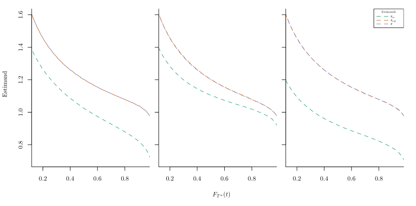
Figure 5: $\theta_{\mathrm{adj}},\theta_{m},\theta$ for the setting in fig. 4, with $\beta_{LA}=0.25$, $T^{a}=T^{0}/U_{1}$, $\lambda^{0}_{i}(t)=\frac{t^{2}}{20}U_{0i}e^{\beta a},U_{0}\sim\Gamma(1,1)$ and $U_{1}$ follows a BHN distribution with $\rho_{1}=1$, $\mathbb{E}[U_{1}]=3^{1/3}$ (($p_{1}$, $\mu_{1}$, $p_{2}$, $\mu_{2}$) = $(0.05,0.5,0.18,3.53)$) and $\tau_{0}=0.5,\tau_{1}=0$ (left); $\tau_{0}=0,\tau_{1}=0.5$ (middle); $\tau_{0}=\tau_{1}=0.5$ (right).

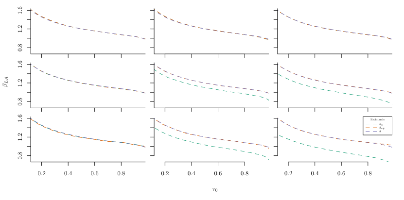
Figure 7: $\theta_{\mathrm{adj}},\theta_{m},\theta$ for the setting in fig. 4, $T^{a}=T^{0}/U_{1}$, $\lambda^{0}_{i}(t)=\frac{t^{2}}{20}U_{0i}e^{\beta a},U_{0}\sim\Gamma(1,1)$, $U_{1}$ follows a BHN distribution with $\rho_{1}=1$, $\mathbb{E}[U_{1}]=3^{1/3}$ (($p_{1}$, $\mu_{1}$, $p_{2}$, $\mu_{2}$) = $(0.05,0.5,0.18,3.53)$), where $\beta_{\mathrm{LA}}\in\{0,0.25,0.45\}$, $\tau_{0}\in\{0,0.25,0.45\}$ and $\tau_{1}=0$.

For the example considered here, confounding resulting from a relation of $L$ with $U_{0}$ results in a larger deviation of $\theta_{m}$ from $\theta$ than due to a relation with $U_{1}$. Obviously, when both relations are present, the deviation is even larger. The larger, $\beta_{\text{AL}}$, $\tau_{0}$ and $\tau_{1}$, the larger the deviation of $\theta_{m}$ from $\theta$ as illustrated in fig. 7-fig. 9 in appendix B. Here it also becomes clear once more that in the absence of confounding ($\beta_{\text{AL}}=0$ or $\tau_{0}=\tau_{1}=0$) $\theta_{m}=\theta$, cf. theorem 3.1.

5 Case study: Federation Francophone de Cancerologie Digestive Group Study 9803

[3] reviewed the properties of and estimation methods for the AFT model and presented a simulation study to discuss the applicability of the AFT model as an alternative to the proportional hazard model in the context of cancer clinical trials. As a practical example, time-invariant semi-parametric AFT models were fitted to the progression-free survival times of 20 trials in advanced gastric cancer (the data is publicly available as supplementary materials in [4]). To verify the appropriateness of the model, and thus the time-invariant effect, the survival function of the residuals $\log T-\log\theta_{m}{\cdot}A$ were compared. A deviation was observed for the trial conducted by [2] with $135$ participants.

We will fit a time-varying AFT model to this data to estimate $\theta_{m}$. Since the sample size is small, we cannot resort to a non-parametric estimator. Instead, we apply the flexible parametric method proposed in [6] as implemented in the aft() function from the R package rstpm2. Using a cubic spline with $3$ degrees of freedom for $\log(-\log S_{T\mid A=1})$ and a cubic spline with two pre-specified knots for $\log\theta_{m}$, the model fits quite well as illustrated in fig. 10 in appendix B. The default output of the aft() function is in terms of $\eta$ (cf. eq. 8), but we have written some additional code to output the estimate of $\theta_{m}$, and its uncertainty. The code for this case study can be found at https://github.com/marbrath/causal_AFT. The estimated $\theta_{m}$ is presented in fig. 6.

Figure 6: Estimated $\theta_{m}$ (solid black) and corresponding $95$% confidence intervals (dashed black) on $F_{T^{1}}$ axis (left) and time axis (right). Furthermore, $\theta$ for for $S_{T^{0}}=S_{T|A=0}$ and $S_{T^{1}}(t)=0.5S_{T^{0}}(0.9t)+0.5S_{T^{0}}(0.45t)$ is presented (purple).

Due to the small sample size, the $\theta_{m}$ curve suffers from serious statistical uncertainty so that a constant acceleration factor cannot be ruled out. In the remaining discussion, we will ignore the statistical uncertainty. One might conclude that there is a time-varying acceleration factor such that the treatment becomes more beneficial in time, i.e. the $F_{T|A=1}(t)$ quantile of $T|A=0$ equals $t\,\theta_{m}(t)$ and thus decreases relative to $t$ over time. As explained in this paper, one can not distinguish such a time-varying causal effect from a time-invariant heterogeneous causal effect.

Interestingly, for the meta-analysis conducted in [17], two treatment arms were merged. These arms contained individuals treated additionally with Cisplatin or Ironotecan ([2]). In the case that these two treatment regimes have different (but homogeneous) effects, there is treatment effect heterogeneity in the merged group. This heterogeneity will result in a time-varying acceleration factor. For example, assume the acceleration factor for Cisplatin is $0.9$ and for Ironotecan is $0.45$, then the survival function for receiving one of these treatments with probability $0.5$ equals $S_{T^{1}}(t)=0.5S_{T^{0}}(0.9t)+0.5S_{T^{0}}(0.45t)$. When $S_{T^{0}}$ equals the $S_{T\mid A=0}$ distribution fitted before, the resulting $\theta$ is presented with the purple line in fig. 6. These time-invariant but heterogeneous effects could quite well explain the estimated time-varying acceleration factor.

6 Discussion

In this work, we have formalized the causal interpretation of the acceleration factor estimand in AFT models, and we have shown that it yields an appropriate causal effect measure in the presence of frailty and treatment effect heterogeneity. If the model is well-specified, the estimated AFT model parameter can thus directly be used to answer a scientific question. In presence of heterogeneity, this does not hold for the parameter of a proportional hazard model, for which one should additionally derive the survival curves corresponding to the fitted model.

The results are restricted to cause-effect relations that can be described by the specified structural causal accelerated failure time model (2). We emphasize the generality of this model, as it leaves $F_{T^{0}}$ unspecified and the time-varying acceleration factor allows for arbitrary relationships between the quantiles of $F_{T^{0}}$ and $F_{T^{a}}$. Note that the validity of (2) can not be verified with data as $F_{(T^{0},T^{a})}$ is not observed. However, we only use the causal mechanism to show what estimands are targeted when fitting a (time-variant) AFT model in the presence of heterogeneity. The validity of the AFT model to describe $F_{T\mid A=0}$ and $F_{T\mid A=a}$ (in absence of confounding equal to $F_{T^{0}}$ and $F_{T^{a}}$) can be verified.

We have revealed that the observed acceleration factor is time-variant when the causal effect is time-invariant but heterogeneous, hence the time-invariant AFT model is misspecified in the presence of effect heterogeneity. Table 2 in appendix B displays empirically obtained estimands $\mathbb{E}[T^{0}]/\mathbb{E}[T^{a}],\,\exp\left(\mathbb{E}[\log T^{0}]-\mathbb{E}[\log T^{a}]\right)$ for all examples presented in this paper. This demonstrates that for misspecified time-invariant AFTs (i.e. $U_{1}$ is present) the estimands of time-invariant AFTs, eq. 14 and eq. 15, can not be viewed as simple and meaningful summary measures of the treatment effect and will depend on the time-to-follow up. Note that in presence of effect heterogeneity, when fitting the misspecified time-invariant AFT model to two studies with different time-to-follow up, two different estimands are targeted so that the results are not comparable. On the other hand, $\theta_{m}(t)$ are the same for both studies and can simply not be identified after the time-to-follow up. Consequently, time-invariant AFTs must be employed if heterogeneity is believed to be present.

As shown in Section 4, the presented results generalize to a setting with confounding, but in the absence of unmeasured confounding, since conditional AFT models can be used to estimate $\theta_{\text{adj}}$ which then equals $\theta$. However, it must be clear that in the presence of confounding $\theta_{m}$ itself does not have a valid causal interpretation. Practitioners should appropriately adjust for confounders and reason why there are no unmeasured confounders to leverage the causal interpretation of the AFT model. In a setting with time-varying treatments, that we do not consider in this work, more sophisticated methods may be necessary to appropriately adjust for time-varying confounding ([8]).

In summary, we have demonstrated that AFT models offer a satisfactory alternative to proportional hazard models due to the interpretability of the estimands. However, we have illustrated that in the presence of effect heterogeneity it is virtually impossible that a time-invariant AFT model is well-specified so that a time-variant model is necessary for accurate causal inference. The practical implementation of the latter may still present a significant hurdle for practitioners.

Appendix A Proofs

A.1 Proof of Theorem 3.1

Proof.

Alternative 1, marginally.
By section 2 it follows that $T^{a}=g(U_{0},U_{1},N_{T},a)$ for some function $g$, hence by the assumption $N_{A}\perp\!\!\!\perp(U_{0},U_{1},N_{T})$ (no confounding), $T^{a}\perp\!\!\!\perp A$. The result then follows by exchangeability and consistency,

$$S_{T^{a}}(t) =\mathbb{P}(T^{a}>t)=\mathbb{P}(T^{a}>t|A=a)=\mathbb{P}(T>t|A=a)=S_{T|A=a}(t).$$

∎

Proof.

Alternative 2, conditionally (on $U_{0},U_{1}$).

$$S_{T^{a}}(t) =\int S_{T^{a}|U_{0}=u_{0},U_{1}=u_{1}}(t)\,dF_{(U_{0},U_{1})}(u_{0},u_{1})$$

$$=\int\mathbb{P}\left(T^{a}>t\,|\,U_{0}=u_{0},U_{1}=u_{1}\right)\,dF_{(U_{0},U_{1})}(u_{0},u_{1})$$

$$=\int\mathbb{P}\left(T^{a}>t\,|\,U_{0}=u_{0},U_{1}=u_{1},A=a\right)\,dF_{(U_{0},U_{1})}(u_{0},u_{1})$$

$$=\int\mathbb{P}\left(T>t\,|\,U_{0}=u_{0},U_{1}=u_{1},A=a\right)\,dF_{(U_{0},U_{1})}(u_{0},u_{1})$$

$$=\int\mathbb{P}\left(T>t\,|\,U_{0}=u_{0},U_{1}=u_{1},A=a\right)\,dF_{(U_{0},U_{1})\mid A=a}(u_{0},u_{1})$$

$$=S_{T|A=a}(t).$$

By using $T^{a}=g(U_{0},U_{1},\varepsilon,a)$ for some function $g$ and the assumption of no confounding, it follows that $T^{a}\perp\!\!\!\perp A\,|\,U_{0},U_{1}$, which yields the third equality. Then the fourth equality follows by consistency. The assumption of no confounding is employed once more in the fifth equality to reach the desired result. ∎

A.2 Proof of Proposition 3.1

Proof.

By use of theorem 3.1 it suffices to show that $S_{T|A=a}(t)=s_{a}(t),S_{T|A=0}(t)=s_{a}(t)$, which is immediate by writing the survival functions on the form

$$S_{T|A=a}(t) =\exp\left(-\int_{0}^{t}\lim_{h\to 0}\frac{1}{h}\mathbb{P}\left(T\in[u,u+h)\,|\,T\geq u,A=a\right)\,du\right),$$

$$S_{T|A=0}(t) =\exp\left(-\int_{0}^{t}\lim_{h\to 0}\frac{1}{h}\mathbb{P}\left(T\in[u,u+h)\,|\,T\geq u,A=0\right)\,du\right),$$

and employing eq. 12. ∎

Appendix B Supplementary figures and tables

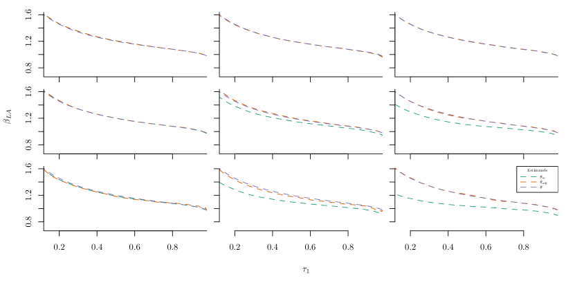
Figure 8: $\theta_{\mathrm{adj}},\theta_{m},\theta$ for the setting in fig. 4, $T^{a}=T^{0}/U_{1}$, $\lambda^{0}_{i}(t)=\frac{t^{2}}{20}U_{0i}e^{\beta a},U_{0}\sim\Gamma(1,1)$, $U_{1}$ follows a BHN distribution with $\rho_{1}=1$, $\mathbb{E}[U_{1}]=3^{1/3}$ (($p_{1}$, $\mu_{1}$, $p_{2}$, $\mu_{2}$) = $(0.05,0.5,0.18,3.53)$), where $\beta_{\mathrm{LA}}\in\{0,0.25,0.45\}$, $\tau_{1}\in\{0,0.25,0.45\}$ and $\tau_{0}=0$.

Figure 9: $\theta_{\mathrm{adj}},\theta_{m},\theta$ for the setting in fig. 4, $T^{a}=T^{0}/U_{1}$, $\lambda^{0}_{i}(t)=\frac{t^{2}}{20}U_{0i}e^{\beta a},U_{0}\sim\Gamma(1,1)$, $U_{1}$ follows a BHN distribution with $\rho_{1}=1$, $\mathbb{E}[U_{1}]=3^{1/3}$ (($p_{1}$, $\mu_{1}$, $p_{2}$, $\mu_{2}$) = $(0.05,0.5,0.18,3.53)$), where $\beta_{\mathrm{LA}}\in\{0,0.25,0.45\}$, $\tau_{1}\in\{0,0.25,0.45\}$ and $\tau_{0}=\tau_{1}$.

Figure 10: Empirical (dashed) and model based (solid) survival functions for the treated ($a=1$) and control ($a=0$) arm.

Example	$T^{0}\sim$	$U_{0}$ dist.	$\mathrm{Var}(U_{0})$	$U_{1}$ dist.	$\mathrm{Var}(U_{1})$	$\mathbb{E}[U_{1}]$	$\mathbb{E}[T^{0}]/\mathbb{E}[T^{1}]$	$\exp\left(\mathbb{E}[\log T^{0}]-\mathbb{E}[\log T^{a}]\right)$
Table 1 (a)	Weibull	Gamma	0.5	degenerate	0	$0.693$	$0.693$	$0.693$
	Weibull	Gamma	1	degenerate	0	$0.693$	$0.693$	$0.693$
	Weibull	Gamma	2	degenerate	0	$0.693$	$0.693$	$0.693$
	Weibull	IG	0.5	degenerate	0	$0.693$	$0.693$	$0.693$
	Weibull	IG	1	degenerate	0	$0.693$	$0.693$	$0.693$
	Weibull	IG	2	degenerate	0	$0.693$	$0.693$	$0.693$
Figure 2 (left)	Weibull	Gamma	1	BHN	1	$0.693$	0.385	0.001
Figure 2 (right)	Weibull mixture	-	-	BHN	1	$0.693$	0.385	0.000
Figure 3	Weibull	Gamma	1	Gamma	0.5	$0.693$	0.023	0.000
	Weibull	Gamma	1	Gamma	1	$0.693$	0.000	0.000
	Weibull	Gamma	1	Gamma	2	$0.693$	0.000	0.000
Table 1 (b)	Weibull	Gamma	0.5	degenerate	0	$1.442$	1.442	1.442
	Weibull	Gamma	1	degenerate	0	$1.442$	1.442	1.442
	Weibull	Gamma	2	degenerate	0	$1.442$	1.442	1.442
	Weibull	IG	0.5	degenerate	0	$1.442$	1.442	1.442
	Weibull	IG	1	degenerate	0	$1.442$	1.442	1.442
	Weibull	IG	2	degenerate	0	$1.442$	1.442	1.442
Figure 2 (left)	Weibull	Gamma	1	BHN	1	$1.442$	1.090	1.477
Figure 2 (right)	Weibull mixture	-	-	BHN	1	$1.442$	1.090	1.572
Figure 3	Weibull	Gamma	1	Gamma	0.5	$1.442$	1.096	1.513
	Weibull	Gamma	1	Gamma	1	$1.442$	0.750	0.206
	Weibull	Gamma	1	Gamma	2	$1.442$	0.128	0.000

Table 2: Empirically obtained estimands ($n_{\mathrm{obs}}=1e6$) for examples considered in paper. $T^{0}\sim\mathrm{Weibull}(60,1/3)$, except for Weibull mixture $T^{0}$, where $T^{0}\sim\mathrm{Weibull}(\Lambda,2),\Lambda\sim X/\Gamma(1+1/2),X$ categorical ($\mathbb{P}(X=1)=\mathbb{P}(X=10)=0.5$). All $U_{0}$ distributions are parametrized such that $\mathbb{E}[U_{0}]=1$.

References

- [1] Odd O Aalen, Richard J Cook and Kjetil Røysland “Does Cox analysis of a randomized survival study yield a causal treatment effect?” In Lifetime data analysis 21 Springer, 2015, pp. 579–593
- [2] Olivier Bouché et al. “Randomized Multicenter Phase II Trial of a Biweekly Regimen of Fluorouracil and Leucovorin (LV5FU2), LV5FU2 Plus Cisplatin, or LV5FU2 Plus Irinotecan in Patients With Previously Untreated Metastatic Gastric Cancer: A Fédération Francophone de Cancérologie Digestive Group Study—FFCD 9803” PMID: 15514373 In Journal of Clinical Oncology 22.21, 2004, pp. 4319–4328 DOI: 10.1200/JCO.2004.01.140
- [3] Tomasz Burzykowski “Semi-parametric accelerated failure-time model: A useful alternative to the proportional-hazards model in cancer clinical trials” In Pharmaceutical Statistics 21.2 Wiley Online Library, 2022, pp. 292–308
- [4] Marc et al. Buyse “Statistical evaluation of surrogate endpoints with examples from cancer clinical trials” In Biometrical Journal 58.1 Wiley Online Library, 2016, pp. 104–132
- [5] David Roxbee Cox and David Oakes “Analysis of survival data” CRC press, 1984
- [6] Michael J et al. Crowther “A flexible parametric accelerated failure time model and the extension to time-dependent acceleration factors” In Biostatistics 24.3 Oxford University Press, 2023, pp. 811–831
- [7] Miguel A Hernán “The hazards of hazard ratios” In Epidemiology 21.1 LWW, 2010, pp. 13–15
- [8] Miguel A Hernán et al. “Structural accelerated failure time models for survival analysis in studies with time-varying treatments” In Pharmacoepidemiology and drug safety 14.7 Wiley Online Library, 2005, pp. 477–491
- [9] Miguel A Hernán and James Robins “Causal inference” CRC Boca Raton, FL, 2010
- [10] Niels Keiding, Per Kragh Andersen and John P Klein “The role of frailty models and accelerated failure time models in describing heterogeneity due to omitted covariates” In Statistics in medicine 16.2 Wiley Online Library, 1997, pp. 215–224
- [11] Torben Martinussen, Stijn Vansteelandt and Per Kragh Andersen “Subtleties in the interpretation of hazard contrasts” In Lifetime Data Analysis 26 Springer, 2020, pp. 833–855
- [12] Menglan Pang, Robert W Platt, Tibor Schuster and Michal Abrahamowicz “Flexible extension of the accelerated failure time model to account for nonlinear and time-dependent effects of covariates on the hazard” In Statistical Methods in Medical Research 30.11 SAGE Publications Sage UK: London, England, 2021, pp. 2526–2542
- [13] Richard AJ Post, Edwin R Heuvel and Hein Putter “Bias of the additive hazard model in the presence of causal effect heterogeneity” In Lifetime Data Analysis Springer, 2024, pp. 1–21
- [14] Richard AJ Post, Edwin R Heuvel and Hein Putter “The built-in selection bias of hazard ratios formalized using structural causal models” In Lifetime Data Analysis Springer, 2024, pp. 1–35
- [15] James Robins and Anastasios A Tsiatis “Semiparametric estimation of an accelerated failure time model with time-dependent covariates” In Biometrika 79.2 Oxford University Press, 1992, pp. 311–319
- [16] The GASTRIC Group “Benefit of adjuvant chemotherapy for resectable gastric cancer: a meta-analysis” In Jama 303.17 American Medical Association, 2010, pp. 1729–1737
- [17] The GASTRIC Group “Role of chemotherapy for advanced/recurrent gastric cancer: An individual-patient-data meta-analysis” In European Journal of Cancer 49.7, 2013, pp. 1565–1577 DOI: https://doi.org/10.1016/j.ejca.2012.12.016
- [18] L.. Wei “The accelerated failure time model: A useful alternative to the cox regression model in survival analysis” In Statistics in Medicine 11.14-15, 1992, pp. 1871–1879 DOI: https://doi.org/10.1002/sim.4780111409