Connectivity Structure and Dynamics of Nonlinear Recurrent Neural Networks
Abstract
We develop a theory to analyze how structure in connectivity shapes the high-dimensional, internally generated activity of nonlinear recurrent neural networks. Using two complementary methods – a path-integral calculation of fluctuations around the saddle point, and a recently introduced two-site cavity approach – we derive analytic expressions that characterize important features of collective activity, including its dimensionality and temporal correlations. To model structure in the coupling matrices of real neural circuits, such as synaptic connectomes obtained through electron microscopy, we introduce the random-mode model, which parameterizes a coupling matrix using random input and output modes and a specified spectrum. This model enables systematic study of the effects of low-dimensional structure in connectivity on neural activity. These effects manifest in features of collective activity, that we calculate, and can be undetectable when analyzing only single-neuron activities. We derive a relation between the effective rank of the coupling matrix and the dimension of activity. By extending the random-mode model, we compare the effects of single-neuron heterogeneity and low-dimensional connectivity. We also investigate the impact of structured overlaps between input and output modes, a feature of biological coupling matrices. Our theory provides tools to relate neural-network architecture and collective dynamics in artificial and biological systems.
I Introduction
Nonlinear recurrent neural networks are used in neuroscience as models of neural-circuit dynamics [1, 2, 3] and in machine learning as systems for sequence processing [4, 5, 6, 7]. Such networks can generate complex, time-varying activity in the absence of external input [8, 9]. This high-dimensional chaotic activity, first analyzed by Sompolinsky et al. [10], has served as a model for asynchronous cortical dynamics observed in vivo. Moreover, initializing recurrent neural networks so that they exhibit chaotic dynamics has been shown to facilitate subsequent learning [11, 12, 13].
Theoretical studies often focus on large recurrent neural networks with independent and identically distributed (i.i.d.) couplings. However, the structure of real-world networks, including neural circuits, typically deviates substantially from this assumption [14]. Many real-world networks show approximate low-rank structure, meaning that their connectivity is well described by a number of rank-one components that is smaller than the number of units in the network [15]. Often, networks have “smooth low-rank” or “effectively low-rank” structure in which the strengths of these rank-one components do not exhibit a hard cutoff and instead decay smoothly, with a more rapid falloff than in networks with i.i.d. couplings. This can arise when connections between units depend on their distance in physical space, or in a low-dimensional feature space [16, 17, 18]. Such low-rank structure can also emerge when artificial neural networks are trained on tasks [19, 20].
To illustrate this, we examined a central-brain connectome of the fruit fly Drosophila melanogaster [21] (Fig. 1a). We estimated strengths from synaptic counts, assigned coupling signs based on predicted neurotransmitter types [22], and normalized the couplings (Fig. 1b; Appendix B). We analyzed the network’s structure using its singular value decomposition (SVD), which expresses the connectivity as a sum of rank-one components, with the strength of each component given by the corresponding singular value. The singular values decay much more quickly than those of an i.i.d. matrix of the same size, which follow a universal form that does not depend on details of the single-element distribution (Fig. 1c). We quantify this decay rate using the participation ratio of the squared singular-value spectrum (Sec. II.4.1). For this connectome, the participation ratio is , much lower than the value of for an i.i.d. matrix, demonstrating that this network has a much lower-rank structure than would be expected for i.i.d. couplings.
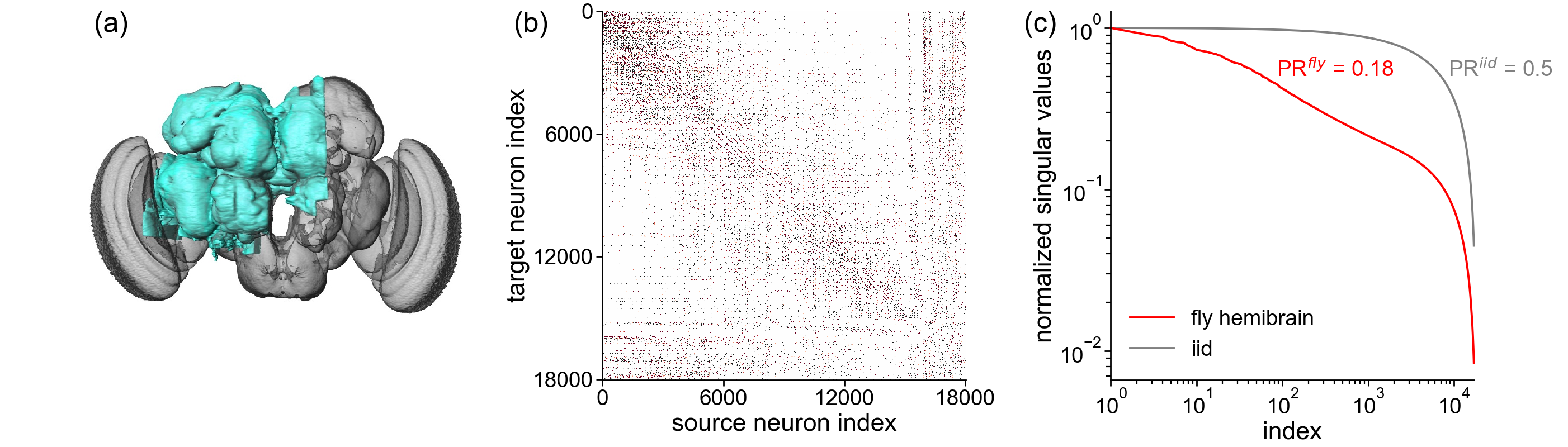
In neuroscience, the importance of connectivity lies in its role in controlling neural activity. To this end, dynamical mean-field theory (DMFT) has been used to analyze activity in large recurrent neural networks, focusing on single-neuron properties such as the autocovariance function. However, recent neuroscience studies have highlighted the significance of geometric or other collective properties that emerge only when examining the simultaneous activity of large neuronal populations [23, 24]. Given neural data, these properties are often analyzed using dimensionality reduction techniques like principal component analysis. Recent advances have extended DMFT techniques to analytically characterize these collective features in nonlinear network models producing high-dimensional chaotic activity [25]. Other studies have addressed simpler cases, including linear networks driven by noise [26, 27, 28, 29] and nonlinear networks producing low-dimensional activity [30, 31]. A key quantity of interest is the dimension of activity, which quantifies the number of high-variance activity modes. This metric reflects a network’s capacity for complex computations and representations, and influences its learning and generalization capabilities [32, 33]. Despite these advances, the analytical calculation of activity dimension in nonlinear networks has been limited to i.i.d. connectivity, or connectivity with simple correlations between reciprocal synapses, and thus cannot be performed for networks with more realistic structures (Fig. 1c). To address this gap, we study networks with smooth low-rank parameterizations of couplings, and develop DMFT tools to analyze collective activity in such networks. We show that, in certain cases, the effects of structure in connectivity are not evident in single-neuron activity, but instead revealed through dramatic changes in properties of collective activity that we show how to compute.
This paper has two main contributions. The first is a new path-integral calculation of a specific four-point function of network activity, originally defined by Clark et al. [25]. This function captures statistics describing collective activity, including its dimensionality. In Secs. II.1–II.3, we describe the recurrent-network model and define this four-point function. We explain its connection to collective activity features, including the activity dimension and timescales of principal components, and review its calculation in i.i.d. networks. In Secs. III.1–III.4, we introduce the new path-integral calculation and apply it to both the i.i.d. model and a model with correlations between reciprocal pairs of synapses.
The second contribution is a tractable model of neural-network coupling matrices that we call the random-mode model. In Sec. II.4, we define this model, in which couplings are generated as a sum of rank-one outer products of random input and output modes with component-specific strengths. In Sec. II.4.1, we demonstrate that parameterizing these strengths provides control over the singular value spectrum of the coupling matrix, enabling investigation of the interplay between global connectivity structure and network dynamics. In Sec. III.5, we calculate the two- and four-point functions for the random-mode model using the path-integral approach. This analysis reveals a bipartite coupling between neurons and latent variables. In Sec. III.6, we interpret the resulting formulas for the four-point function, which show how the effective rank of the coupling matrix controls the dimension of activity. In Sec. IV, we analyze limiting cases of the random-mode model, illustrating that a vanishing effective rank leads to vanishing activity dimension. In Sec. V, we show that the same results can be obtained using an intuitive two-site cavity method. In Sec. VI, we study the behavior of a generalization of the random-mode model featuring heterogeneity among single-neuron properties and contrast the effects with those of low-rank structure in the connectivity. Finally, in Sec. VII, we incorporate a simple form of overlaps between input and output modes into the model, which we anticipate to be crucial for describing neural computations.
II Model and summary statistics
II.1 Recurrent neural network model
We study a recurrent neural network of neurons. Each neuron is characterized by its pre-activation and activation , where . The activations are related to the pre-activations through a nonlinear function , with . While our results are agnostic to the form of the nonlinearity, when comparing theory and simulations we use , which is similar to the more conventional but allows for analytical evaluation of Gaussian integrals. The network dynamics are governed by
| (1) |
where is the coupling from neuron to neuron , and is a causal functional describing single-neuron dynamics. A canonical choice is
| (2) |
resulting in low-pass filtering of the input. We measure time in units of the time constant that would appear in front of .
II.2 Correlation functions
II.2.1 Two-point functions
To characterize the network dynamics, we introduce several types of two-point correlation functions. Let denote either the pre-activations or activations. We first define the neuron- and time-averaged covariance:
| (3) |
We also define the time-averaged, but not neuron-averaged, covariance; and the neuron-averaged, but not time-averaged, covariance:
| (4) | ||||
| (5) |
For a given , the spectra of , with indices and , and of , with indices and , are the same (up to a scaling), so spectral properties of one parameter can be computed using the other, a form of duality. For example, the properly scaled trace operations applied to these parameters yield the same result, namely, .
We also define the response function:
| (6) |
where is an infinitesimal source term added to the right-hand side of the network dynamics (Eq. 1). In analogy with the covariance functions, we define , , and to be the response function averaged over time, neurons, or both.
II.2.2 Four-point functions
To characterize the dimension and timescales of activity, we define
| (7) |
where . This sum includes the on-diagonal contributions, unlike the quantity computed in Clark et al. [25], which we denote by the lower-case :
| (8) |
For the type of connectivity we will study, the network exhibits high-dimensional activity such that pairwise covariances are . Thus, in the definition of (Eq. 7), the on-diagonal contributions (given by ) and off-diagonal contributions (given by ) are both .
II.2.3 Relating to the dimension and timescales of activity
The dimension of activity can be quantified by the participation ratio of its covariance spectrum [34, 35, 23, 36, 32, 37, 9, 38, 27]. To define the participation ratio, we diagonalize the equal-time covariance matrix to obtain eigenvectors and eigenvalues , as in principal components analysis. The participation ratio is
| (10) |
where we normalized by to obtain an intensive, self-averaging quantity. To see why this provides a useful measure of dimension, consider the case where a fraction of eigenvalues are equal to a positive constant and the rest are zero. Then, . In practice, the spectrum often has a smooth decay with characteristic decay constant rather than a hard cutoff. In this case the spectrum takes the form , leading to where is an order-one constant. Thus, the participation ratio picks out the characteristic decay scale [36].
An advantageous property of this dimension measure is that it can be expressed in terms of the previously defined two- and four-point correlation functions as
| (11) |
Recall that for the types of connectivity we study, cross-covariances are , so the on- and off-diagonal contributions to are both order-one (Eq. 7). This leads to taking a value between 0 and 1 as . Thus, the unnormalized dimension of activity is extensive, i.e., activity is high-dimensional. At the same time, activity does not uniformly occupy all available dimensions, which would require cross-covariances to be smaller than .
Timescales of collective activity can be studied as follows. We define the principal components (PCs) of network activity as
| (12) |
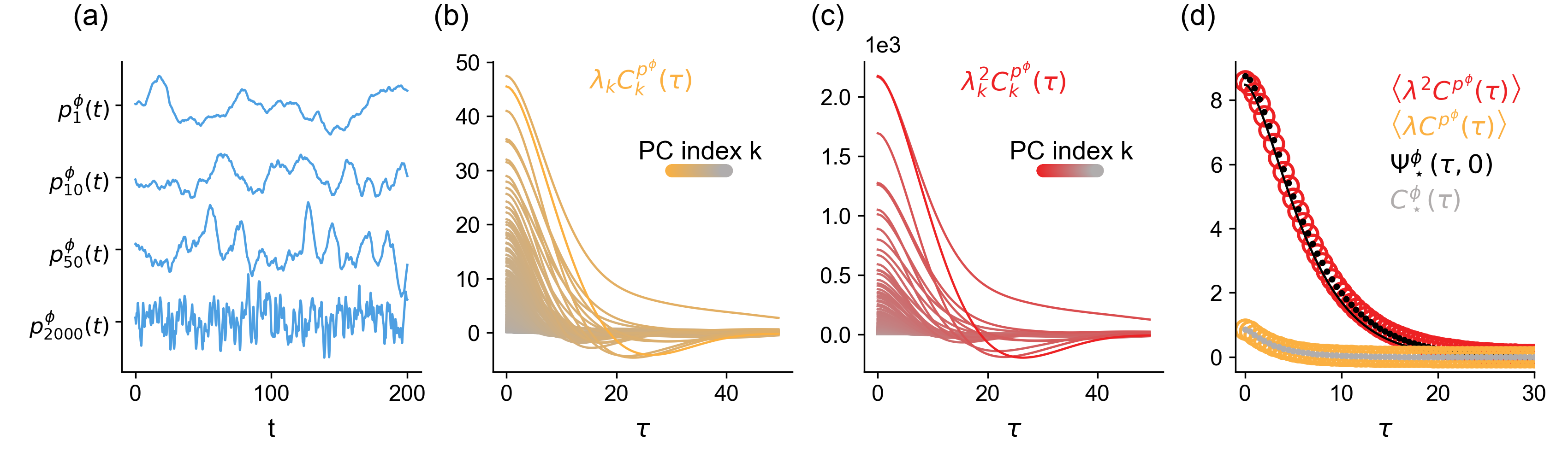
These PCs are the basis of much of modern analysis of high-dimensional neural data. The PCs all have unit variance but potentially very different characteristic timescales (Fig. 2a). To extract the timescales of just the leading PCs, we compute the PC-averaged covariance, weighted by the squares of the eigenvalues of the corresponding PCs. This gives:
| (13) |
showing that captures the temporal structure of the leading PCs of network activity (Fig. 2c,d). Note that weighting by the eigenvalues themselves, rather than their squares, gives , recovering single-neuron information (Fig. 2b,d).
II.3 Computing the two- and four-point functions in the i.i.d. case
We now review how to compute these two- and four-point functions in a classic network model with i.i.d. couplings . The first- and second-order coupling statistics are:
| (14) |
The magnitude of a typical coupling is . We refer to as the coupling strength. For the canonical dynamics of Eq. 2, the network is quiescent for and chaotic for , with a sharp phase transition as . In this paper we assume that the network is non-quiescent.
We compute and in the limit under the disorder average. We use the subscript to denote such limiting, disorder-averaged values:
| (15) | ||||
| (16) |
These values also correspond to the saddle point of a path integral. Both of these functions are self-averaging, meaning that the same values are obtained, up to fluctuations, when they are computed based on a single realization of a large network. In this paper, we are interested in statistically stationary, temporally fluctuating states such that .
The two-point function can be computed through a single-site picture that describes the dynamics of a typical neuron embedded in the rest of the network, with pre-activation and activation . The single-site dynamics are given by
| (17) |
where is a Gaussian field with mean zero and covariance . We denote this by
| (18) |
is determined self-consistently by enforcing
| (19) |
where denotes an average within this single-site process, i.e., with respect to the Gaussian distribution of . Once has been determined, follows easily. This single-site problem can be derived through either a single-site cavity calculation (see [39]) or a saddle-point condition in a path integral (see [40, 41]). For the i.i.d. couplings considered here, there is a simpler heuristic derivation: in the neuronal input , the correlations between the couplings and dynamic variables can be safely neglected to leading order in , yielding both Gaussianity of by the central limit theorem and the second-order statistics of Eq. 18.
Clark et al. [25] first computed using a dynamic, two-site version of the cavity method, based on the neuron-by-neuron definition (Eq. 7). This method finds , the off-diagonal contribution to , noting that the on-diagonal contribution is simply . A cavity is first created by removing two neurons from the network and allowing the rest of the network, the reservoir, to generate dynamic activity. The cavity neurons are then introduced, and their effect on the reservoir is treated perturbatively. This yields a pair of coupled mean-field equations for the cavity units, generalizing the single-site picture discussed above to a two-site picture. Finally, self-consistency conditions are constructed by recognizing that the cavity pair is statistically equivalent to any reservoir pair. This calculation results in expressions for the four-point function in Fourier space, given by
| (20) |
for the activations, and
| (21a) | ||||
| (21b) | ||||
for the pre-activations, where and is a cross-covariance between the pre-activation and activation. Note that if the joint distribution of pre-activations were Gaussian, and would differ only by a proportionality constant due to Price’s theorem [42]. The more complex relationship observed here reflects the non-Gaussian joint statistics across different neurons, which is relevant because the network is nonlinear.
II.4 Definition of the random-mode model
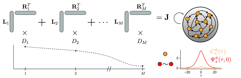
Many studies have examined the dynamics of networks with i.i.d. couplings, as described in the previous section. However, the coupling matrices of real-world networks often have approximate low-rank spectral structure, deviating dramatically from the i.i.d. assumption. To analyze networks with such properties, we introduce the random-mode model. This model generates a coupling matrix of the form
| (22) |
where and are “input” and “output” modes in the neuron space and is a weighting factor called the component strength. The effect of multiplying by is to project a neuronal activity vector onto , scale it by , project the result along , and sum these contributions for all (Fig. 3, top). Eq. 22 can be written
| (23) |
where and are matrices and .
A crucial modeling choice is how the number of modes, , scales relative to the network size, . We consider the limit where both and approach infinity while maintaining a fixed ratio,
| (24) |
This scaling results in extensive-rank connectivity, meaning that the rank of grows linearly with . Importantly, choosing to be small (or choosing the component strengths to decay rapidly; see below) allows for connectivity that is low-rank compared to the number of neurons.
For now, we assume that the matrices and have independent and identically distributed elements with zero mean and variance . We assume these elements are Gaussian, although our results should not depend on the exact form of the single-element density for large due to the central limit theorem.
A key feature of the random-mode model is that we have full control over the component strengths , which are analogous to the singular values of (we make this link precise in Sec. II.4.1). We assume only that these component strengths follow a distribution that remains constant as grows, ensuring a well-defined large- limit. By varying this distribution, we can explore the impact of the spectral structure of the connectivity on collective features of network activity (Fig. 3, bottom).
We denote the -th moment of the distribution by
| (25) |
It will be useful to define the participation ratio,
| (26) |
from which we define the “effective rank” of the couplings,
| (27) |
This quantity is related to the participation ratio of the singular value spectrum of via Eq. 28 below. We will show that this effective rank is a key feature of that controls the collective activity structure.
II.4.1 Relationship to singular value decomposition
The random-mode model has similarities to the SVD, which decomposes a rank- matrix as . Here, and are matrices whose columns are the left and right singular vectors (or modes), respectively, and is a diagonal matrix containing the singular values, . The left singular vectors are orthonormal among themselves, as are the right singular vectors (although the left and right singular vectors are generally not orthonormal to each other). In contrast, the columns of and in the random-mode model have i.i.d. statistics, resulting in random, overlaps among both within- and across-matrix columns. This i.i.d. assumption offers analytical tractability by eliminating the need to enforce orthonormality, a complicated global constraint (but see [43], who handle random orthonormal matrices in a regression setting). Furthermore, by not explicitly modeling overlaps between and , the random-mode model parameterizes using only the component strengths , although such overlaps can be introduced (see Sec. VII).
Given a matrix drawn from the random-mode model, we can examine the relationship between the singular values, , and the component strengths, . The non-orthonormality of and introduces some discrepancy between the two sets of values. We first compare the participation ratio of the squared singular value spectrum, , to the effective rank, . We find:
| (28) |
where , and are the singular values of . This follows from using Wick’s theorem to evaluate the expectations of and for the numerator and denominator, respectively, of . For , demonstrating that the component strengths are closely related to the singular values in the low-dimensional regime. In this regime, the random modes approximate an orthonormal set of vectors as since the overlaps between modes can be neglected when there are few of them. While we express the analytic results in this paper in terms of , Eq. 28 can always be used to translate between and .
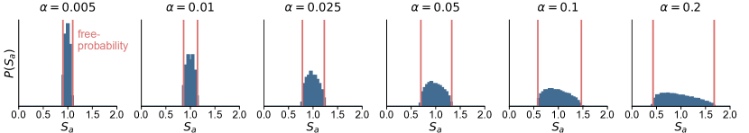
We further quantify the discrepancy between singular values and component strengths in the case where for all . Using methods from free probability theory [44, 45], we compute that the singular values are distributed over a range with boundaries
| (29) |
This is in agreement with large- simulations (Fig. 4). For small , While the random-mode model spreads the nonzero singular values over a range, this spreading becomes negligible for small . More generally, the distributions of and coincide for small .
II.4.2 Comparison to low-rank recurrent neural networks
A related parameterization of connectivity has been explored in low-rank recurrent neural networks, where the coupling matrix is expressed as a sum of outer products of input modes and output modes :
| (30) |
with being the connectivity rank [30, 46, 31, 47]. In some instances, this low-rank component is added to an i.i.d. matrix modeling unstructured “background” connectivity [30, 46].
Several features separate this approach from the random-mode model. Low-rank recurrent neural networks maintain a constant rank as , yielding intensive-rank connectivity that models low-dimensional activity, whereas the random-mode model uses extensive-rank connectivity, modeling high-dimensional activity. Furthermore, low-rank recurrent neural networks allow for the most general possible parameterization of overlaps between modes, captured by a overlap matrix . Specifying such overlaps in the random-mode model would require parameters, comparable to defining the full coupling matrix. To reduce parameter complexity, the random-mode model specifies only the variances of mode components via the component strengths , disregarding overlaps. This substantially reduces parameter count while preserving interesting network dynamics. In Sec. VII, we introduce additional parameters describing a restricted overlap structure among modes, specifying only diagonal elements of the overlap matrix. Further possible overlap forms are discussed in Sec. VIII.
The mean-field descriptions of network dynamics produced by these connectivities also differ markedly. In low-rank recurrent neural networks, low-dimensional network activity is described by a finite set of order parameters representing projections of network activity onto input modes , obeying effective nonlinear dynamics. Conversely, the extensive-rank connectivity in the random-mode model generates high-dimensional chaotic activity, described by covariance functions capturing temporal fluctuations. While the random-mode model’s mean-field analysis introduces latent variables given by projections of network activity onto input modes, their extensive number precludes their use as order parameters.
A final distinction lies in the scaling of the coupling matrix and its implications for the alignment of activity with connectivity. In low-rank recurrent neural networks, elements of scale as and the input-output mode overlaps are , resulting in strong alignment of network activity with input modes. This is reminiscent of the rich regime of neural networks [48, 49, 50, 51]. Conversely, in the random-mode model, the elements of scale as and the input-output mode overlaps are , leading to weak alignment of network activity with any given input mode; the pre-activations are since each neuron combines input from modes. This is reminiscent of the lazy regime of neural networks [49, 52, 53].
III Path-integral calculation of the two- and four-point functions
The path-integral approach provides a systematic framework for analyzing neural-network dynamics, allowing for controlled approximations such as expansions [54, 55, 41, 56]. In this section, we demonstrate how to formulate the calculation of the four-point function within this formalism, allowing us to solve complex models more efficiently than the two-site cavity method by following a straightforward procedure whose steps we outline at the end of Sec. III.3.
III.1 Relating to fluctuations of the time-by-time covariance
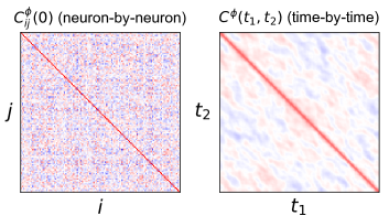
To cast the problem in the language of path integrals, we turn to the time-by-time definition of , given by Eq. 9. If the time-by-time covariance were equal to its limiting value, , we would have since, for large time differences, , decays exponentially in [10]. However, based on the neuron-by-neuron definition, Eq. 7, is clearly a nonzero, order-one quantity. This apparent contradiction is resolved by considering fluctuations around the saddle point. The necessity of these fluctuations becomes clear when viewed through the lens of neuron-time duality. The presence of nonzero pairwise covariances indicates low-dimensional structure in the system. Equivalently, this structure manifests as the system revisiting similar states in phase space over time, resulting in nonzero temporal covariance even for large time differences (Fig. 5). To capture this behavior, we define fluctuations around the saddle point as
| (31) |
We express purely in terms of these fluctuations as
| (32) |
noting that terms involving vanish at large time differences. Our task, therefore, is to compute the covariance of the fluctuations, , captured by
| (33) |
Then, to compute , we use the temporal limits
| (34) | ||||||
III.2 Path-integral formalism and two-point functions
Given any fixed , we express the network dynamics using a path integral in the Martin–Siggia–Rose/Janssen–De Dominicis–Peliti formalism [57]:
| (35) |
where suppressed time indices imply time integrals, e.g., . Here, is a field conjugate to that enforces the network’s equations of motion (Eq. 1). This path integral serves as a generating function for moments of dynamic variables: by adding source terms to the action, derivatives of with respect to and produce correlation and response functions, respectively (these sources are not needed for our purposes). In this paper, we keep track of the path integral up to non-physically meaningful multiplicative factors. For a review of this path-integral formalism applied to neural networks, see [40, 41, 58]. To obtain the typical behavior, we average over , yielding a disorder-averaged path integral .
For simplicity, we begin with the i.i.d. model of with mean zero and variance . After performing the Gaussian integration over , we introduce an auxiliary field , defined by Eq. 5, and its conjugate to factorize the action across the neuron index . This leads to a partition function for a statistical field theory involving and :
| (36) |
where the intensive action is
| (37) |
and the single-site path integral is
| (38) |
In the limit , the saddle point dominates this integral. The derivatives of the action, which are zero at the saddle point, are
| (39) | ||||
| (40) |
where denotes an average within the dynamic process described by . In evaluating derivatives of the action, we follow the rule that derivatives with respect to also affect , and likewise for , due to the symmetry in the action. Using the vanishing of correlation functions involving only the conjugate field , the saddle-point conditions yield
| (41) | ||||
| (42) |
where denotes an average within the dynamic process described by . This recovers the same single-site process (Eq. 17, Eq. 18) and self-consistency condition (Eq. 19) described in Sec. II.3.
III.3 Four-point functions
We now compute within the path-integral formalism. Fluctuations around the saddle point derived above are governed by the Hessian of the action [40, 59]. This Hessian has blocks given by
| (43a) | ||||
| (43b) | ||||
| (43c) | ||||
where , . Expanding the action to second order around the saddle point, the path integral becomes
| (44) | |||
revealing the structure of the Gaussian fluctuations around the saddle point. The covariance matrix among the fluctuation variables, and , is times the inverse Hessian, yielding
| (45) | |||
In principle, we have all the necessary components to evaluate this expression: the single-site dynamics are known via the saddle-point condition, and the Hessian blocks are given in terms of connected correlation functions in this single-site process. We could then take the temporal separation limits of Eq. 34 to obtain . The challenge is that each Hessian block is a complicated time2-by-time2 matrix that, for general values of the time variables, has no analytic inverse. To circumvent this problem, we show in Appendix C that the temporal limits of Eq. 34 can be taken before taking the inverses. Under these temporal limits, the Hessian blocks are
| (46) | |||
| (47) | |||
| (48) |
where we used the fact that multiplication by is equivalent to a functional derivative with respect to a source at time . Since the relevant quantities are now translation-invariant, i.e., depend only on and , we can transform to Fourier space. In this representation, each Hessian block becomes a frequency-dependent scalar,
| (49) | ||||
| (50) | ||||
| (51) |
In summary, the full Hessian can be replaced by a two-by-two, frequency-dependent Hesssian given by
| (52) |
where we simplified notation by suppressing frequency arguments via the shorthand and . The Fourier-space function is the upper-left element of the inverse of this matrix. Performing the two-by-two matrix inversion gives
| (53) |
which agrees with the two-site cavity result (Eq. 20).
To summarize, we compute through the following steps (in the next section, we show how to compute ):
-
1.
Write down the path integral, integrate out disorder, and introduce two-point fields and conjugate partners to factorize the action along extensive indices.
-
2.
Sovle the saddle-point equations of the resulting action, yielding the covariance and response functions.
-
3.
Derive the frequency-dependent Hessian by computing second derivatives of the action with respect to the two-point fields, applying the temporal limits of Eq. 34, and transforming to Fourier space. Then, determine the element of the inverse frequency-dependent Hessian corresponding to .
This approach allows for the efficient calculation of two- and four-point functions for a given model, requiring only a few lines of computation directly from the action of the theory. To demonstrate the flexibility of the path-integral approach in computing , we apply it to compute for a generalization of the i.i.d. model in which there are correlations between reciprocal couplings, recovering the result in [25] from the two-site cavity method (Appendix E).
III.4 Adding sources
Above, computing was simplified by appearing naturally in the statistical field theory resulting from integrating out . To compute , we need to introduce a source-field term in the action.
Consider a general intensive action where is a collection of fields (e.g., ), and is a source. In Appendix D, we show that
| (54) |
with all quantities evaluated at the saddle point. By applying this formula to the action of the i.i.d. model with the source term added to the single-site path integral (Eq. 38), we recover the expression for from the two-site cavity method (Clark et al. [25]; Eq. 21). For actions of the form , this formula reduces to as expected.
III.5 Path-integral analysis of the random-mode model
Having demonstrated the path-integral approach to computing two- and four-point functions in well known connectivity models, we now apply this formalism to the random-mode model. In terms of the mode matrices and , the path integral is
| (55) |
We would like to integrate out and , but this is complicated by them appearing together in a quadratic term in the action. To simplify the integration, we introduce a set of latent variables,
| (56) |
and their conjugates . We use indices for neurons and for latent variables. The introduction of these latent variables makes the action linear in and :
| (57) |
We can now easily integrate out and . To factorize the action over indices spanning extensive dimensions, we introduce the field (Eq. 5) with conjugate as well as
| (58) |
with conjugate . The disorder-averaged path integral is
| (59) | ||||
| (60) | ||||
| (61) | ||||
| (62) |
Thus, analysis of the path integral is made tractable by recasting the problem as interacting neurons and latent variables. The neuronal single-site picture is described by , and the latent-variable single-site picture is described by , where the subscript reflects that each latent variable has its own component strength. This formulation introduces an extensive set of latent variables , in contrast to the finite set of latent variables, conventionally denoted by , in low-rank neural networks [30, 31]. The statistics of the Gaussian input to each single-site process (neurons or latent variables) are determined by the statistics of the other process, creating a bipartite, mutually referential structure that also arises in the cavity treatment of the problem.
III.5.1 Two-point functions
Following the steps outlined at the end of Sec. III.3, we first compute the DMFT by calculating the saddle point. The derivatives of the action are
| (63) | ||||
| (64) | ||||
| (65) | ||||
| (66) |
where and are averages within the dynamic processes described by and , respectively. Setting these derivatives to zero yields
| (67) | ||||
| (68) | ||||
| (69) |
where and are averages within the dynamic processes described by and , respectively. These single-site processes are
| (70) | ||||
| (71) |
where and are Gaussian fields,
| (72) | ||||
| (73) |
showing that the neuronal and latent-variable single-site processes have mutually referential statistics 111Note that the variance of is scaled by ; equivalently, we could factor out from the variance and include as a multiplicative factor in the latent-variable single-site dynamics (Eq. 71).
Solving for by combining Eq. 69, Eq. 71, and Eq. 73, we obtain with defined by Eq. 25. Consolidating these results, the self-consistent problem that determines can be expressed purely in terms of this correlation function as
Comparing to Eqs. 17–19, we recover the self-consistent equations of the i.i.d. model with coupling strength
| (74) |
Thus, the low-rank coupling structure remains undetectable at the single-neuron level, where neurons experience effectively i.i.d. connections with variance . The structure of the random-mode model emerges only in collective neural activity, as we now demonstrate by calculating the four-point function.
III.5.2 Four-point functions
The frequency-dependent saddle-point Hessian is
| (75) |
The upper-left block, corresponding to the latent variables, is related to the Hessian of an i.i.d. network with linear dynamics and a heterogeneous distribution of single-neuron scale factors ; the lower-right block, corresponding to the neurons, is related to the Hessian of an i.i.d. network of nonlinear neurons (Eq. 52). They are coupled through the simple off-diagonal blocks, reflecting the interaction between neurons and latent variables. Finally, we obtain for the four-point function:
| (76) |
To obtain , we add to the neuronal single-site path integral (Eq. 61) and compute
| (77) |
Inserting these into Eq. 54 and using a formula (Eq. 149) to invert the Hessian, we obtain
| (78) |
where (Eq. 21b with ).
III.6 Interpreting the formulas
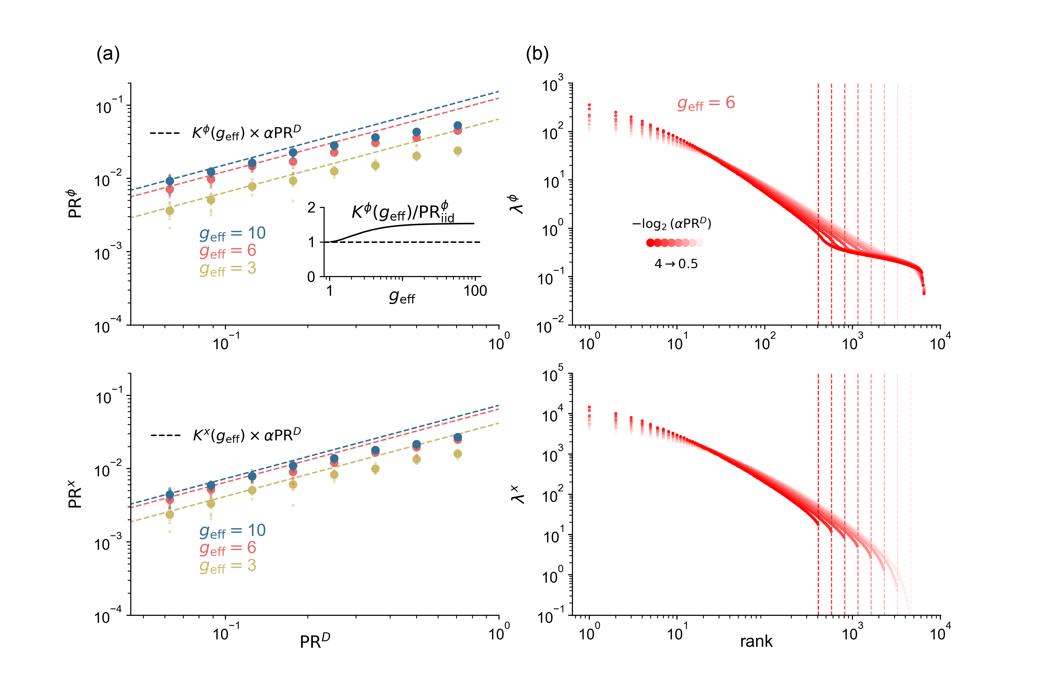
The analytic formulas for the four-point function of the random-mode model (Eq. 76 and Eq. 78) reveal several insights. Taking the limit for fixed , which leads to elements of being i.i.d., recovers the known formulas for i.i.d. couplings (Eq. 20 and Eq. 21). Comparing to the i.i.d. formulas, any structure beyond i.i.d. connectivity (i.e., being finite) strictly decreases the dimension of activity.
Our analysis reveals two key statistical features of the connectivity that characterize how connectivity shapes activity: the effective coupling strength, , and the effective rank, . The first characterizes the typical magnitude of couplings, while the second characterizes global information about the number of significant connectivity components. As in the i.i.d. model, influences both single-neuron activity (described by ) and collective activity (described by ). In contrast, influences collective activity exclusively. The random-mode model therefore provides independent control over single-neuron and collective aspects of activity.
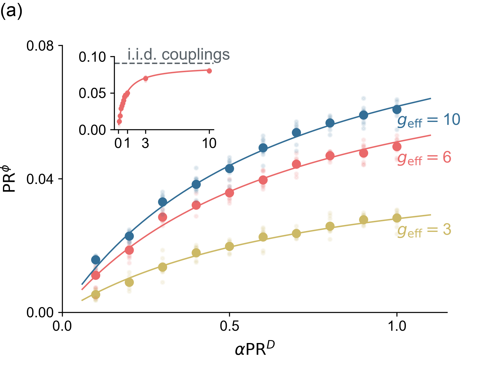
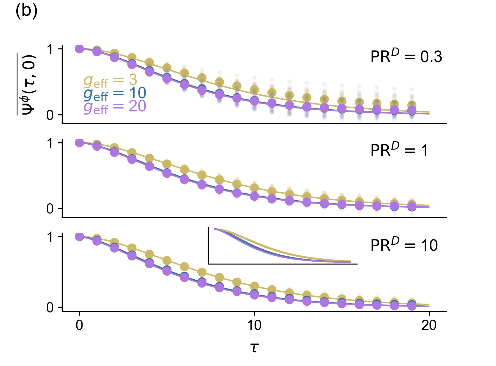
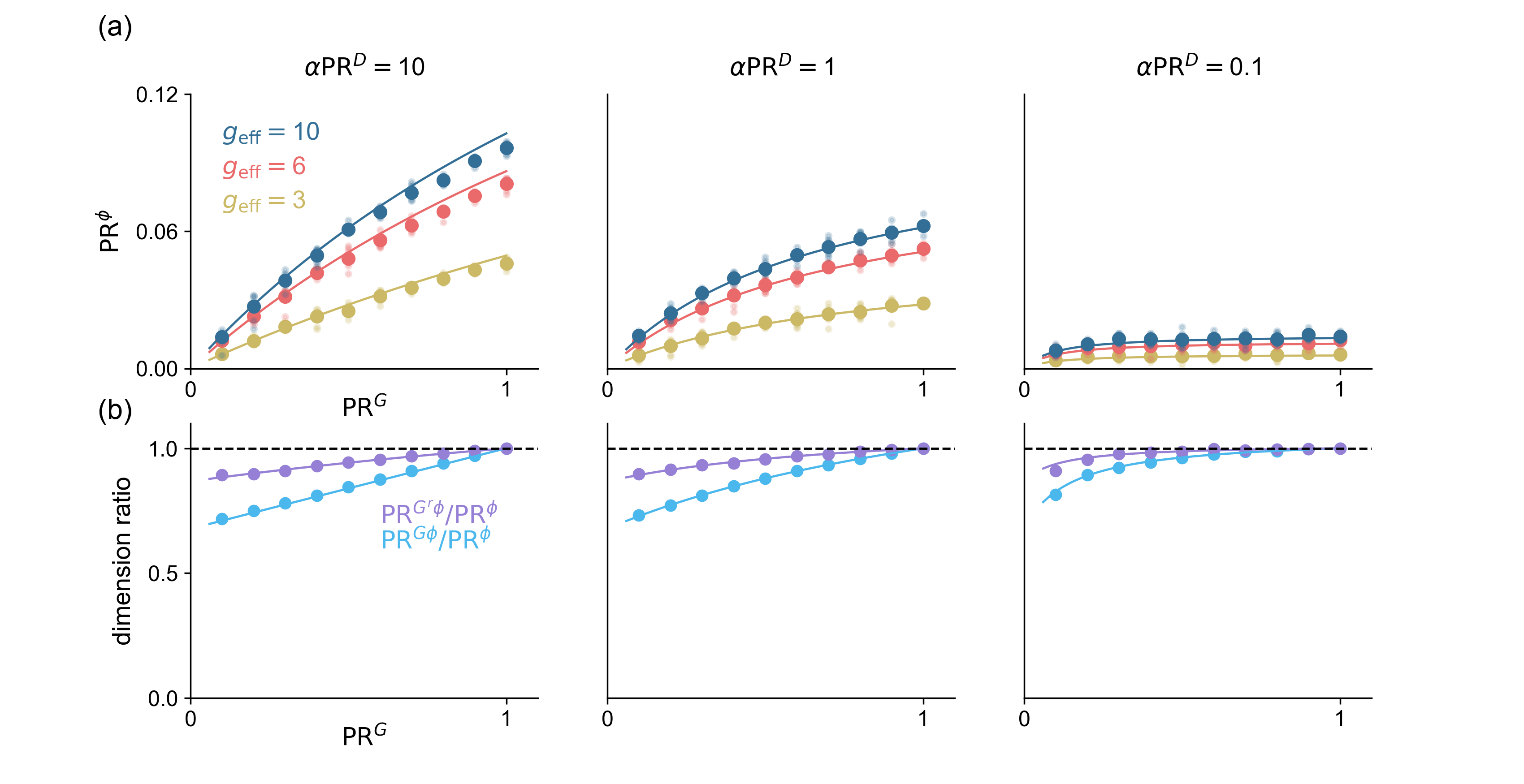
To validate the theoretical prediction for (Eq. 76), we simulated networks and computed the participation ratio from the empirical equal-time covariance matrix of the activations. For the component strengths , we used a spectrum given by
| (79) |
for , which yields . The corresponding density is with support on . To attain a desired effective rank , we set and solved for . For , we fixed and increased . We adjusted by rescaling (i.e., adjusting the proportionality constant in Eq. 79).
Our simulations show excellent agreement with theoretical predictions across parameter settings (Fig. 6). Fig. 6a illustrates how the dimension of activity, , varies with for different values of . Consistent with i.i.d.-coupling networks, increases monotonically with [25]. It also increases monotonically with , approaching the dimension of a network with i.i.d. couplings for large (Fig. 6a inset). As approaches zero, the dimension of activity also approaches zero. We examine the limits and in detail in Sec. IV.
Beyond the dimension of activity, which depends on at , we also examined the temporal profile of this function. Fig. 6b shows a normalized version of , which is related to the correlation functions of leading principal components, for various values of and . The decay timescale of decreases with increasing , approaching a limiting behavior at . While affects the overall scale of this function, and consequently the dimension of activity, it has little effect on the decay timescale, and thus little effect on the timescales of leading principal components (Fig. 6b, inset). Thus, the effective rank primarily influences the dimension of activity rather than the collective temporal structure.
IV Limiting behavior of the random-mode model
Here we examine the behavior of the random-mode model in two limiting cases: as the system approaches the transition to chaos from above (), and in the limit of low effective rank ().
We first consider approaching the transition to chaos from above, i.e., . The relevant expansion parameter is . For networks with i.i.d. couplings, Clark et al. [25] showed that, for coupling strength , and in this limit. For the random-mode model, to leading order in , we have
| (80) |
Consequently, to leading order in , the dimension of activity behaves as
| (81) |
Thus, as the network approaches the transition to chaos, the effect of structure in connectivity is to reduce the dimension by a factor of compared to a network with i.i.d. couplings. Taking the further limit of yields the simple relation
| (82) |
The difference between and is a higher-order correction, so we also have
| (83) |
That is, in the limits of both low effective rank and small effective coupling strength, the dimension of activity is equal to the dimension of the singular-value spectrum times the dimension of activity in an i.i.d. network.
We now consider the limit of low effective rank, , for arbitrary . In this limit, the component strengths closely approximate the singular values of the coupling matrix. To leading order in ,
| (84) |
where
| (85) | ||||
| (86) |
We match this theory of limiting behavior to simulated networks with and a step function for the component strengths:
| (87) |
We varied and verified its linear relationships with and in the limit (Fig. 7a).
Focusing on , note that its expression (Eq. 85) resembles the formula for the dimension of activity in a i.i.d. network with coupling strength , but includes an additional factor in the integral (compare to Eq. 20). Numerical evaluation of shows that it approaches as as expected from Eq. 82. As increases, increases monotonically to approximately (Fig. 7a, inset). These results show that for networks with low effective rank, up to an order-one fudge factor that becomes exactly one as .
We also investigated the relationship between the eigenvalues of and the component strengths . In the low-effective-rank limit, the quantities and computed from these spectra exhibit a linear relationship (with proportionality factor ), implying that the ratio of their second-squared and fourth moments are tightly linked. However, we find that the full forms of the eigenvalue and component-strength spectra differ markedly. Whereas the component strengths decay according to a step function in this example, the rank-ordered eigenvalues and decay smoothly (Fig. 7b). Thus, the dynamics transform the connectivity spectrum into an activity spectrum with a different form while preserving the linear relationship between and .
V Cavity analysis of the random-mode model
While the path-integral approach provides a systematic framework for analyzing neural-network dynamics, the cavity method offers an intuitive, complementary perspective. This section provides an overview of the cavity analysis for the random-mode model, with the full mathematical details available in Appendix G. While these approaches yield equivalent results, they differ in their methodology: the path-integral approach focuses on fluctuations around the saddle point in a field theory, whereas the cavity approach examines perturbations induced by a subset of held-out variables.
Leveraging Eq. 56, we reformulate the network as a bipartite system of neurons and latent variables and extend the cavity calculation of Clark et al. [25] to both groups. This leads to separate, mutually referential cavity pictures for each group, mirroring the two single-site path integrals (Sec. III.5). As in the path-integral formalism, self-consistent expressions in one picture are defined using averages from the other. Unlike the path-integral approach, which derives using its time-by-time definition (Eq. 9), the cavity method derives this function using its neuron-by-neuron definition (Eq. 7).
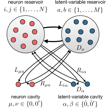
The cavity method we employ, schematized in Fig. 8, has two key features that distinguish it from simpler cavity calculations. First, it uses a two-site structure: we consider the simultaneous removal of two neurons, or two latent variables, from the network, rather than just one. This allows us to study pairwise correlations between neurons. This approach was previously used in Clark et al. [25]. Second, it incorporates a bipartite structure: we treat both neurons and latent variables as dynamic objects, creating separate but mutually referential cavity pictures for each group. Such bipartite structure, without the two-site structure, has been used in cavity calculations in the Hopfield model [61, 62]. Note that these two features are distinct: the two-site aspect refers to the number of neurons removed in each cavity, while the bipartite aspect refers to the types of variables considered (neurons and latent variables).
VI Single-neuron heterogeneity
While the random-mode model introduces heterogeneity in connectivity through the component strengths , individual neurons may also exhibit heterogeneous properties. For instance, cortical neurons display a broad distribution of mean firing rates [63]. To compare the effects of low-dimensional structure in connectivity with the effects of heterogeneous neuronal properties, we extend our analysis to networks with diverse single-neuron characteristics.
In particular, we generalize the neuronal nonlinearity to , which depends on a vector of parameters . The parameter vector for the -th neuron, , is sampled i.i.d. from a distribution . This formulation allows us to model diverse neuronal properties such as gains or biases. When analyzing neural data, it is common to normalize neuronal activities (e.g., through -scoring) to put them on the same scale. To facilitate analysis of such normalized activations, we also introduce a set of variables that do not depend on .
We incorporate the generalized nonlinearity into the path integral, as well as a source term for the normalized variables, and integrate out and . To factorize the action over indices spanning extensive dimensions, we introduce, among others, the order parameter
| (88) |
where . In Appendix H, we derive a single-site dynamic process , where , with the self-consistency condition
| (89) |
This condition is identical to that of an i.i.d. network, but with an average over , in addition to the usual Gaussian average over , to account for single-neuron heterogeneity.
To write down the solution the solution for the four-point function, we define new two-frequency correlation functions with an outer average over :
| (90a) | ||||
| (90b) | ||||
| (90c) | ||||
along with the usual shorthand . For the unnormalized variables , we obtain
| (91) |
For the normalized variables , we obtain
| (92) |
where .
VI.1 Diverse single-neuron firing rates
An illustrative case of single-neuron heterogeneity occurs when the parameters consist of a gain parameter for each neuron, modeling diversity in mean firing rates:
| (93) |
In this scenario, the dynamics of the network are determined by an effective coupling matrix , where . This extension of the random-mode model allows us to directly compare the effects of low-dimensional structure in the connectivity (via the component strengths ) with heterogeneity in single-neuron properties (via the gains ). We assume the gains are drawn from a distribution with moments
| (94) |
To quantify the heterogeneity in firing rates, we define the participation ratio of the gain distribution:
| (95) |
We analyze collective activity for both the unnormalized activations and the normalized activations . The latter are analogous to -scored firing rates in neural recordings, where -scoring removes single-neuron heterogeneity while preserving nontrivial structure due to cross-neuron and temporal correlations.
For the unnormalized variables, we calculate the four-point function
| (96) |
and for the normalized variables,
| (97) |
where
| (98) | ||||
| (99) |
Eq. 97 demonstrates that reductions in effective rank, described by , and in the heterogeneity of gains, described by , have symmetric effects on the dimension of normalized activity, with their combined effect captured by the harmonic mean, . This symmetry arises because swapping the distributions of and does not change the spectrum of when and are i.i.d., since and have the same nonzero eigenvalues. One might expect that normalizing the activations before computing the dimension of activity would remove the effect of heterogeneous gains on the dimension. This is not the case, however, since neuronal gains affect the recurrent dynamics, and not merely the readout.
To further explore this and related effects, we compare the activity dimensions for three sets of activations: (1) unnormalized activations, ; (2) normalized activations, ; and (3) normalized activations multiplied by an independent set of “readout” gains, , where the readout gains have the same distribution as the actual gains. Case (3) corresponds to variables with the same distribution of firing rates as the unnormalized activations, but where this heterogeneity is unrelated to the recurrent dynamics. In this case, we have . The four-point function is
| (100) |
To validate our theoretical predictions (Eq. 96, Eq. 97, and Eq. 100), we simulated networks with component strengths and gains given by
| (101) | ||||
| (102) |
The dimension of activity in these networks is determined by the coupling strength, ; the effective rank of the coupling matrix, ; and the participation ratio of the single-neuron gain distribution, . Increases in each of these parameters leads to higher activity dimension for all three sets of activations.
Normalized activations consistently exhibit the highest dimension. While scaling normalized activations by heterogeneous factors reduces dimension as expected, the magnitude of this reduction depends on whether or is used, even when their distributions are identical. This occurs because neurons with the largest gains preferentially participate in the leading modes of the normalized activations. Further scaling these already-dominant neurons by their gains results in overrepresentation of these neurons compared to using random gains. Thus, the dimension of unnormalized activations is lowest, with the dimension of random-readout activations falling between those of the normalized and unnormalized activations. This effect demonstrates that shuffling the normalizations of recorded neural activities should increase the dimension if firing rates and input covariances are related to one another, as they are in recurrent networks. Not observing such an increase in dimension, on the other hand, would suggest that heterogeneity in firing rates is unrelated to input covariance.
VII Mode overlaps
Thus far, we have assumed that the matrices and are independent of each other. Under this assumption, the overlap between input mode and output mode is a random, quantity. However, to implement computations, modes must interact, suggesting that the coupling matrices of real neural circuits have larger, structured overlaps between input and output modes.
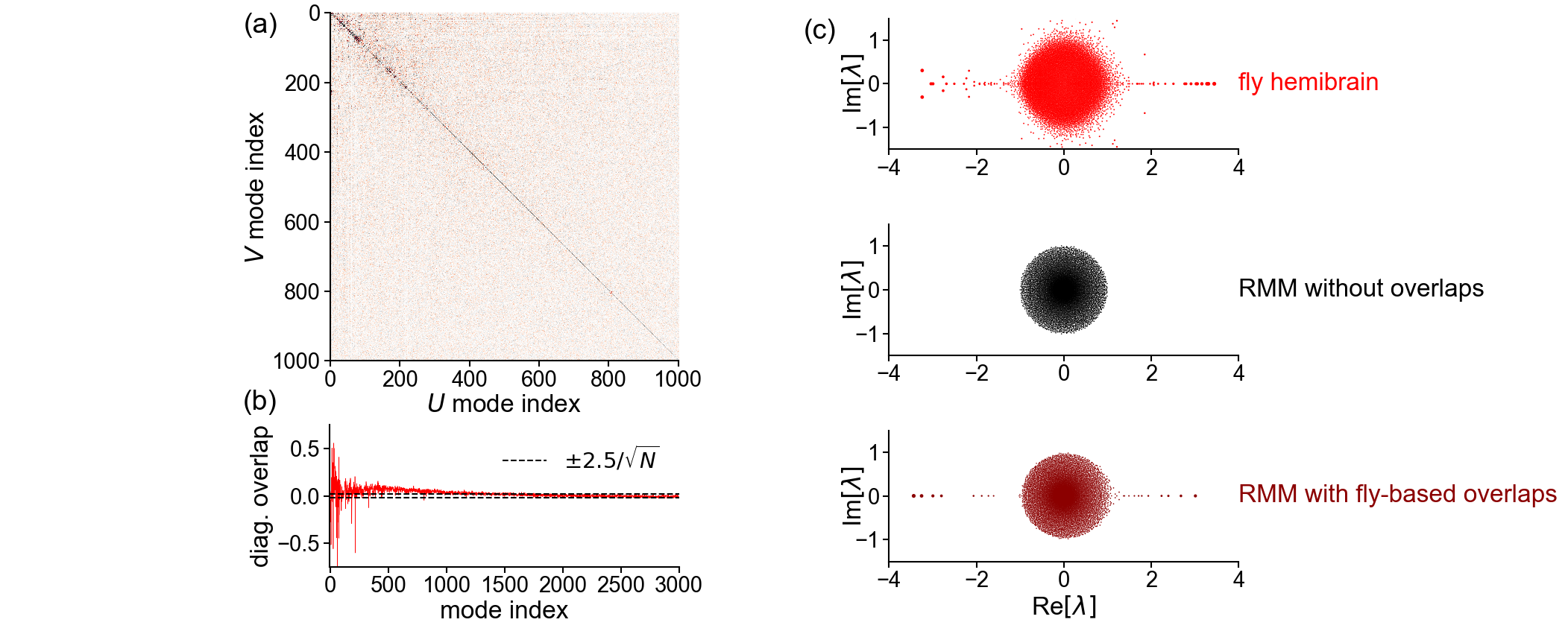
To examine interactions between different modes in a real neural circuit, we returned to the connectome of Drosophila melanogaster. We computed the overlap matrix between its right and left singular vectors, which correspond to the input and output modes, respectively. Rather than the unstructured, overlaps expected from i.i.d. random modes, we observe structured, large overlaps (Fig. 10a). These large overlaps are particularly pronounced near the diagonal of the overlap matrix (Fig. 10b).
Motivated by these observations, we now extend the random-mode model to incorporate structured overlaps between input and output modes. Specifically, we define and as zero-mean Gaussian matrices with the following covariance structure:
| (103) | ||||
| (104) | ||||
| (105) |
where is the overlap matrix. In this case,
| (106) |
To capture the most salient feature of the fly connectome, large diagonal overlaps, we specialize to a diagonal form for the overlap matrix:
| (107) |
where is the correlation between the -th input and output modes. This form of the overlaps implies that, for large , , while for remains a random quantity. Incorporating this structure allows the random-mode model to more accurately match the eigenspectrum of the connectome, which has large outliers along the real axis (Fig. 10c).
Defining an instance of this connectivity with a well-defined large- limit requires specifying a joint distribution from which are sampled for each . Our analytic expressions for the two- and four-point functions depend on averages over this distribution. Note that for large , self-connections (autapses) in are given by
| (108) |
which is, in general, . To avoid biologically unrealistic strong self-connections, one can choose , in which case is random and . Alternatively, if one interprets each model neuron as a cluster of biological neurons, strong self-connections can be interpreted as aggregated within-cluster connectivity [64, 65]. Furthermore, note that the covariance between reciprocal pairs of couplings is given by () where
| (109) |
We compute the two- and four-point functions using the path integral (Appendix I). As in previous cases, we obtain single-site processes for both neurons and latent variables. The neuronal single-site process is given by
| (110) |
where and denotes convolution. The input covariance and convolutional kernel are defined in terms of statistics of the latent-variable single-site process. Due to the linearity of the latent-variable dynamics, we can express them as
| (111) | ||||
| (112) |
We enforce and , yielding a self-consistent system that determines and . Unlike previous cases, there is no effective coupling strength describing the relationship between and ; instead, this relationship involves a convolution with a kernel defined using the joint distribution over . This can be viewed as a frequency-dependent effective coupling strength.
Expanding the self-coupling kernel (Eq. 112) in powers of yields the first two terms
| (113) |
The first term is what we get in the single-site picture for i.i.d. cross-neuron couplings and deterministic self couplings. The second term appears in the single-site picture if there are correlations between reciprocal pairs of couplings, but the structure is otherwise i.i.d. (Appendix E). Nonzero higher-order terms reflect that the structure of the random-mode model is not fully captured by either of these forms. Note that the first two terms being zero forces all subsequent terms to be zero. Thus, nonzero covariance among reciprocal pairs of couplings is a necessary and sufficient condition for attaining a nonzero self-coupling kernel in the single-site picture.
To compute the four-point function, we write down and invert the frequency-dependent Hessian, and obtain
| (114a) | ||||
| (114b) | ||||
| (114c) | ||||
| (114d) | ||||
| (114e) | ||||
| (114f) | ||||
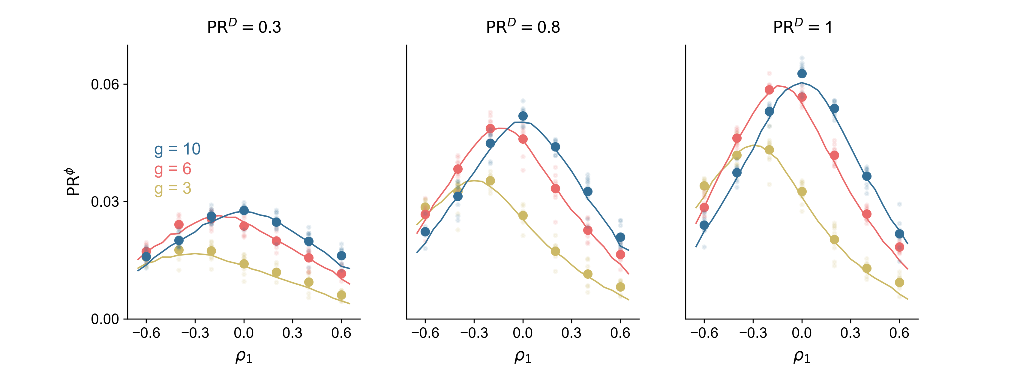
We validated this theory by choosing parameterizations of and . We used and for the component strengths, as before. For the overlaps , we use a sigmoidal shape inspired by Fig. 10b in which the leading components have larger input-output mode overlaps. In particular, we used
| (115) |
which varies from to , hitting at . We fixed , varied , and set such that , eliminating strong self couplings. Across values of and , sufficiently strong overlaps of either sign reduce activity dimension (Fig. 11). The maximum dimension occurs for , a regime in which activity projected along connectivity modes with the greatest strength is most strongly suppressed by the recurrent dynamics. This leftward shift is reduced for larger .
VIII Discussion
A key question in neuroscience and machine learning is how learning shapes collective dynamics through modifications of a neural network’s connectivity. While our analysis has focused on disordered networks that generate chaotic activity and are not trained to perform tasks, the smooth low-rank connectivity structure we have explored provides a starting point for understanding the impact of learned coupling matrices on collective dynamics. Recent works have shown that large neural networks trained on real-world tasks exhibit smooth spectral structures in their coupling matrices, similar to those we have studied [20]. Moreover, while networks trained on simple tasks often display low-rank updates to their initial couplings, with a finite number of outlier eigenvalues emerging from the bulk [19, 46], training networks on many tasks, as is increasingly common, may produce coupling matrices with a low but extensive number of significant components [66, 67]. In such scenarios, the random-mode model, or extensions of it, may predict the resulting activity dimension and other aspects of collective dynamics. The path-integral formalism we have developed is also amenable to analyzing cases where the coupling matrix is drawn from a Gibbs ensemble with an energy function equal to the loss function for a task. This approach represents scenarios where couplings are trained to minimize a loss function with stochastic gradient descent [52]. Finally, initializing couplings with low-rank structure could improve training procedures like FORCE learning, which are based on suppressing chaos, because the initial strange attractor is lower-dimensional [11, 12].
Historically, neural connectivity was often characterized through network motifs – recurring patterns like cycles or chains among small neuronal groups [68, 14, 69, 70]. Such local statistics can be estimated using connectivity datasets obtained from methods that sample subsets of synapses. However, recent advances in whole-brain connectome reconstruction have unveiled global synaptic connectivity structures [71]. These connectomes reveal a more complex picture, where the spectrum and modes of the connectivity matrix exhibit large-scale structure that cannot be explained by local motifs [72]. Our parameterization of coupling matrices attempts to describe this global perspective, offering control over both the spectrum and mode overlaps. This could be particularly valuable in interpreting large-scale recordings of neural activity in the context of known anatomical connectivity.
In a similar vein, Tiberi et al. [72] proposed a random matrix theory approach for noise-driven linear networks based on parameterizing the eigendecomposition of . By contrast, our use of a DMFT approach allows us to describe nonlinear dynamics. Their parameterization also does not capture relationships between eigenvalues and eigenvectors, which are likely crucial for computations. Our parameterization, which is more akin to an SVD than an eigendecomposition, allows for a simultaneous parameterization of component strengths and corresponding mode overlaps. Other parameterizations of connectivity similar to the random-mode model have been used to study the relationship between spiking and rate-based recurrent networks [73] and to train spiking networks more efficiently [74].
Our description of single-neuron heterogeneity, where each neuron is parameterized by an arbitrary vector , can be readily applied to explore how various forms of heterogeneity influence dimensionality and other features of collective activity. Introducing specific forms of heterogeneity constrained by observed electrophysiological properties [75] and other cell-specific characteristics across neurons could provide insight on the functional consequences of neuronal diversity [76].
On the technical side, we have demonstrated that the two-site cavity method and the analysis of fluctuations around the saddle point in the path integral approach yield equivalent results for computing the four-point function. This equivalence implies that the intricate cavity construction is equivalent to computing and inverting the Hessian of the action in the path integral. A deeper understanding of the relationship between these methods could lead to new hybrid approaches that combine the strengths of both techniques.
In conclusion, the random-mode model and associated analytical techniques provide a set of tools for exploring the relationship between connectivity and collective dynamics. Our parameterization of connectivity is a middle ground between deterministic low-rank models and completely random networks. Future work incorporating more complex mode interactions, diverse neuronal properties, and learning dynamics will further bridge neural connectivity, activity, and function.
Acknowledgements
We gratefully acknowledge L.F. Abbott for discussions and feedback on this work.
Appendix A Glossary of Terms
- Number of neurons ()
-
Total number of neurons in the network.
- Number of modes ()
-
Number of components in the random-mode model.
- (Effective) coupling strength (, )
- Random-mode model
-
Network connectivity model: (Eq. 22).
- Connectivity component ()
-
Outer product of output and input modes.
- Input mode ()
-
Neuronal pattern in the -th component onto which activity patterns are projected.
- Output mode ()
-
Neuronal pattern in the -th component along which the projected activity pattern is expanded.
- Component strength ()
-
Scaling factor for the -th component.
- Ratio of modes to neurons ()
-
Given by (Eq. 24).
- Participation ratio of component strengths ()
- Effective rank ()
-
Connectivity dimensionality measure (Eq. 27).
- Two-point function
-
Correlation function given by (Eq. 5).
- Four-point function
Appendix B Preprocessing of the fly hemibrain connectome
We used the dataset originally presented in Scheffer et al. [21]. To form the connection matrix for analysis, we used synaptic counts as a measure of connection strength, determining the magnitudes of the matrix elements. Neurons were assigned neurotransmitter probabilities based on a machine-learning analysis applied to the electron-microscopy data [22]. We selected the most probable neurotransmitter assignment for each neuron. The neurotransmitter types were then mapped to signs (excitatory or inhibitory) according to Table 1.
To normalize the connectivity matrix, we used an iterative scaling procedure analogous to the Sinkhorn–Knopp algorithm that proceeds as follows. We first rescale the positive elements in each row by a row-specific factor, such that the L2-norm of the positive elements is . The same procedure is applied to the negative elements, using a separate row-specific factor. This results in each row having a L2-norm of one with balanced excitatory and inhibitory inputs. A small number of neurons with exclusively excitatory or inhibitory inputs are left with an L2-norm of instead of one. Following the row normalization, we perform the same operations on the columns. This disrupts the previous row normalization. Thus, we iterate the row and column normalization steps in an alternating fashion until convergence was achieved. The final result is a matrix with proper scaling along both rows and columns, which we interpret as the projection of the original matrix onto the set of properly row- and column-normalized matrices. Importantly, it has the same nonzero elements with the same signs as the original matrix.
| Neurotransmitter | Synaptic Sign |
|---|---|
| GABA | -1 (Inhibitory) |
| Acetylcholine | +1 (Excitatory) |
| Glutamate | -1 (Inhibitory) |
| Serotonin | Ignored |
| Octopamine | Ignored |
| Dopamine | Ignored |
| Neither | Ignored |
Appendix C Temporal limits and inverses
Here, we demonstrate, for the i.i.d. model that the temporal limits in Eq. 34 can be taken before the inverses. This allows us to work with a frequency-dependent Hessian. In this section, we use Einstein notation for integrals over time variables (i.e., repeated time indices are integrated over). We would like to evaluate
| (116) |
in the limits Eq. 34, where and (note that due to the vanishing of correlation functions involving only the conjugate field). Restating Eq. 43, we have
| (117) | ||||
| (118) |
We assume temporal stationarity throughout this section and consider only .
We start by examining the properties of . vanishes if one of the four time points is far (measured on the timescale of ) from the other three. For or , this is a consequence of the perturbation associated with or being far away; for or , this is a consequence of separating from the expectation. also vanishes if there is more than one time point which is far from the remaining ones by the same arguments. Thus, the time points need to be close in pairs. However, if are close and are close, but the pairs are distant, still vanishes since the perturbations associated with are both far. This leaves three possibilities for a non-vanishing : close and close, but the pairs are distant; close and close, but the pairs are distant; or all time points are close.
Separating the three possibilities into two subdomains where all time points are close () and where the time points belong to either of the two pairwise separate () possibilities, we write where and are defined to vanish on the respective other domain. On the separated domain, simplifies to
| (119) |
where we used that the two distant contributions are non-overlapping to add them.
We assume that we can also decompose the inverse into a contribution for separate pairs and a contribution where all time points are close, , where again and vanish on the respective other domain. We demonstrate that is the inverse of , and that is the inverse of , by noting that reduces to the contraction of and if and , and hence and , are close; or to the contraction of and if and , and hence and , are distant.
For Eq. 116, we need due to the limits Eq. 34. The fact that reduces to in the limits Eq. 34 justifies taking the limits before inverting . Furthermore, these limits imply that, in Eq. 116, and , as well as and , are far apart. In this case, simplifies to
| (120) |
This justifies taking the limits Eq. 34 for .
Appendix D Incorporating sources
This section outlines the general approach for incorporating source terms and then applies it to the specific case of correlations among the pre-activations. Our goal is to compute
| (121) |
which gives the fluctuations around the mean of the quantity multiplying in the action. To facilitate this calculation, we introduce a new field and set it equal to using the conjugate :
| (122) |
Instead of taking the second derivative with respect to , we set and compute the fluctuations of in the augmented theory whose path integral is
| (123) |
where
| (124) |
The Hessian of the augmented action, in terms of the Hessian of the original action, is
| (125) |
where
| (126) |
The fluctuations of are given by the bottom-right element of the inverse Hessian evaluated at the saddle point. Using a Schur complement to compute this element, we obtain the expression Eq. 54 stated in the main text.
We now apply Eq. 54 to the action of the i.i.d. connectivity model with a source term for correlations among pre-activations. The action is
| (127) |
Computing the necessary quantities and taking the temporal limits of Eq. 34, we obtain, in Fourier space,
| (128) |
where and . Substituting these into Eq. 54 and using the frequency-dependent Hessian from Eq. 52, we obtain
| (129) |
in agreement with the two-site cavity result of Clark et al. [25], given in Eq. 21.
Appendix E Partially symmetric disorder
To demonstrate the flexibility of the path-integral approach to computing the four-point function, we now consider a generalization of the classic i.i.d. model in which we introduce correlations between reciprocal couplings, characterized by the following statistics:
| (130) |
Here, is a parameter that controls the degree of symmetry in the connectivity. When , the connectivity is fully symmetric, while corresponds to fully antisymmetric connectivity. The case recovers the i.i.d. model. We express this partially symmetric connectivity as a linear combination of two matrices, and , that are i.i.d. random with mean zero and variance :
| (131) |
where . In terms of and , the path integral for this partially symmetric model is
| (132) |
We integrate out and . To factorize the action over indices spanning extensive dimensions, we introduce
| (133) | |||||
| (134) |
We obtain, for the disorder-averaged path integral,
| (135) | ||||
| (136) | ||||
| (137) |
To obtain the saddle-point solution, we compute the derivatives of the action, under the rule that derivatives with respect to also affect , and vice versa, due to the symmetry in the action. This gives
| (138) | ||||
| (139) | ||||
| (140) | ||||
| (141) |
Setting these derivatives to zero yields the saddle-point conditions:
| (142) | ||||
| (143) | ||||
| (144) |
where denotes an average within the dynamic process described by . The single-site process at the saddle point is described by
| (145) | ||||
| (146) |
where denotes convolution. The symmetric structure provides a convolutional, nonlinear self-coupling in the single-site dynamics. The two-point correlation and response functions, and , must be determined self-consistently within this single site picture.
Introducing the notation , for , the frequency-dependent Hessian at the saddle point is
| (147) |
Inverting this matrix and isolating the upper-left element, we obtain, in agreement with Clark et al. [25],
| (148) |
Appendix F Inverse formula
In Sec. III.5.2 and Appendix H, we use the fact that
| (149) |
Appendix G Two-site cavity calculation of the four-point function in the random-mode model
To apply cavity techniques, we reformulate the network as a bipartite system of neurons and latent variables,
| (150) | ||||
| (151) |
as done in the path-integral approach. In the two-site cavity calculation, we keep track various intermediate quantities to order , leading to an expression for accurate to leading order (order one), which we identify as .
To distinguish between different types of variables and their indices, we use the following notation. Neurons are indexed by and latent variables by , as usual. For the cavity variables, we introduce special indices: neuronal cavity variables are indexed by , while latent cavity variables are indexed by .
G.1 Neuronal cavity
We begin by introducing two neurons, and . The leading-order () effect on the latent variables is
| (152) |
where is the response function of the latent variables. The dynamic equations for the cavity neurons are
| (153) |
where
| (154) | ||||
| (155) |
Defining the cavity-field time-average cross-covariance as
| (156) |
we obtain the following expression for the cross-covariance of the cavity units, up to order :
| (157) |
Our goal is to compute the parameter
| (158) |
where denotes an average over , , and . To evaluate this, we need to square and disorder-average Eq. 157. This requires us to consider several two-frequency correlation functions, which we define as
| (159) | ||||
| (160) | ||||
| (161) | ||||
| (162) |
These have all been scaled to be order-one. We can evaluate these functions due to the independence of the couplings and dynamic variables in the expressions defining them, which is a consequence of the cavity construction. Of these, the only nonvanishing ones are
| (163) | ||||
| (164) |
where denote the indices in the latent-variable cavity picture.
G.2 Latent-variable cavity
We now introduce two new latent variables, and . The leading-order () effect on the neurons is
| (165) |
where is the response function of the neurons. The dynamic equations for the cavity latent variables are
| (166) |
where
| (167) | ||||
| (168) |
Defining the time-average cavity-field cross-covariance as
| (169) |
we obtain the following expression for the cross-covariance of the cavity latent variables up to order :
| (170) |
We aim to compute the parameter
| (171) |
by squaring and disorder-averaging Eq. 170. This requires us to consider several two-frequency correlation functions, which we define as
| (172) | ||||
| (173) | ||||
| (174) | ||||
| (175) |
Again, we can evaluate these functions due to the independence of the couplings and dynamic variables in the expressions defining them. The nonvanishing ones are
| (176) | ||||
| (177) |
where denote the indices in the neuronal cavity picture.
G.3 Combining the two two-site cavity pictures
To combine the results from both two-site cavity pictures, we use the following relations:
| (178) | ||||
| (179) | ||||
| (180) |
Using these relations and the definitions of the functions (Eqs. 159-162 and 172–175), we obtain
| (181) | ||||
| (182) | ||||
| (183) | ||||
| (184) |
We solve Eq. 182 and Eq. 184 simultaneously, yielding
| (185) | ||||
| (186) |
With these solutions, we express and in terms of the functions. Switching to frequency-suppressed notation,
| (187) | ||||
| (188) |
Now, we substitute Eq. 187 into Eq. 188. Using , we obtain
| (189) |
where we used the previously defined quantities and . Eq. 189 can be solved for , yielding
| (190) |
This result is identical to Eq. 76 derived using the path-integral approach, demonstrating the consistency between the two methods.
Appendix H Single-unit heterogeneity calculations
The full set of order parameters is
| (191) | |||||
| (192) |
The action and single-site path integrals for this system are
| (193) | ||||
| (194) | ||||
| (195) |
The saddle-point calculation proceeds similarly to the non-heterogeneous case of the random-mode model. We obtain
| (196) | ||||
| (197) | ||||
| (198) |
where and are averages with respect to and , respectively (note that does not depend on ). Using and, consequently, , the self-consistent problem that determines is given by Eq. 89 and the preceding description in Sec. VI.
The frequency-dependent Hessian at the saddle point is
| (199) |
where the new raktur variables are defined in Eq. 90. We invert the Hessian using Eq. 149 and identify the upper-left element as Eq. 91. Combining the inverted Hessian with the relevant quantities for computing fluctuations of normalized variables,
| (200) |
where
| (201) | ||||
| (202) |
we obtain Eq. 92.
Appendix I Structured mode overlaps calculations
To generate matrices and with the correlation structure of Eq. 106 and Eq. 107, we express them in terms of independent Gaussian random matrices and , each with variance :
| (203) | ||||
| (204) |
We begin with the path integral containing latent variables, insert this parameterization of and , then and integrate out , , and . To factorize the action over indices spanning extensive dimensions, we introduce
| (205) | |||||
| (206) | |||||
| (207) | |||||
| (208) |
The resulting path integral, action, and single-site path integrals are given by:
| (209) | ||||
| (210) | ||||
| (211) | ||||
| (212) | ||||
| (213) |
We first calculate the saddle point conditions by taking the derivatives of the action:
| (214) | ||||
| (215) | ||||
| (216) | ||||
| (217) | ||||
| (218) | ||||
| (219) | ||||
| (220) | ||||
| (221) |
The saddle-point conditions yield:
| (222) | ||||
| (223) | ||||
| (224) | ||||
| (225) | ||||
| (226) |
where and are averages within the dynamic processes described by and , respectively. The yields neuronal and latent-variable single-site processes described by
| (227) | ||||
| (228) |
where the Gaussian fields have statistics
| (229) | ||||
| (230) |
This gives rise to the single-site problem described in Sec. VII.
The frequency-dependent Hessian at the saddle point is
| (231) |
where
| (232) | ||||
| (233) | ||||
| (234) | ||||
| (235) | ||||
| (236) |
Isolating the upper-left element of the inverse of this matrix yields Eq. 114.
Appendix J Numerical details
J.1 Numerics for theory
To validate the theory, we used networks with dynamics defined by (Eq. 2) and with nonlinearity . For all connectivity models, except those with structured - overlaps (VII), the single-site two-point functions and depend only on and can be numerically calculated as in i.i.d. networks (see, e.g., [10, 77]). In summary:
-
1.
Since is Gaussian, so is for this linear form of , allowing us to write in terms of Gaussian integrals over and , which have marginal variance and covariance . Due to our choice of , this expression simplifies to
(237) -
2.
Squaring the single-site picture gives a second-order ODE . Since the rhs depends only on and , we can consider it to be the negative derivative of a potential with an explicit dependence on the initial condition .
-
3.
The rhs is integrated w.r.t. to provide an expression for , which due to our choice of simplifies to
(238) -
4.
Restricting to solutions with as and , enforcing conservation of energy gives , which can be solved for by numerical root finding.
-
5.
Finally, Euler integration of the dynamics with these initial conditions gives its full time course, along with via Eq. 237.
We integrated the Newtonian ODE from to with step size . When then use an FFT to otain the frequency-space representation. The frequency-space representation of the response function was computed directly as
| (239) |
with . Various expressions for were then computed in frequency space before transforming back to the time domain by a 2D inverse FFT.
For structured - overlaps, the self-coupling in the single-site process makes non-Gaussian, preventing the use of Gaussian integrals in the DMFT solution. We there obtain the solution via standard numerical methods, enforcing self-consistency among the autocovariance function, ; the self-coupling kernel, ; the response function, ; and the autocovariance function, . In summary:
-
1.
Seed values for kernels are set as and .
-
2.
and are computed in Fourier space using the current values of and via Eq. 112, with the average taken over .
-
3.
A set of instances of are sampled according to the Gaussian process kernel by standard spectral methods.
-
4.
Each of single-site processes is Euler integrated according to Eq. 110 with the input and self-feedback by the convolution between and .
-
5.
These time series and are used to compute empirical values for the autocovariance and response. The latter is computed by the Furutsu-Novikov theorem: . The numerator is estimated using these time series, while is simply .
-
6.
After repetitions of steps (1)-(5) with smoothed updates
(240) (241) as new seed values for the upcoming th iteration, the final numerical estimates for and are computed as the averages over the last iterations.
We used a temporal discretization , . With these quantities, the various components of Eq. 114 and the expression for are straightforward to compute. We took averages in this case by averaging over every other discrete value of and .
J.2 Simulation details
Each network was integrated via Runga-Kutta (RK4) with . The empirical lagged covariance matrix was computed by averaging over individual covariance estimates, each of which is based on discrete, evenly spaced time samples , with :
| (242) |
The value of varied but was generally and always chosen to ensure saturated dimension values, i.e. . Specific quantities of interest, such as or , were computed using this estimate.
References
- Barak et al. [2013] O. Barak, D. Sussillo, R. Romo, M. Tsodyks, and L. Abbott, From fixed points to chaos: three models of delayed discrimination, Progress in neurobiology 103, 214 (2013).
- Mante et al. [2013] V. Mante, D. Sussillo, K. V. Shenoy, and W. T. Newsome, Context-dependent computation by recurrent dynamics in prefrontal cortex, nature 503, 78 (2013).
- Sussillo et al. [2015] D. Sussillo, M. M. Churchland, M. T. Kaufman, and K. V. Shenoy, A neural network that finds a naturalistic solution for the production of muscle activity, Nature neuroscience 18, 1025 (2015).
- Hochreiter and Schmidhuber [1997] S. Hochreiter and J. Schmidhuber, Long short-term memory, Neural computation 9, 1735 (1997).
- Sutskever et al. [2014] I. Sutskever, O. Vinyals, and Q. V. Le, Sequence to sequence learning with neural networks, Advances in neural information processing systems 27 (2014).
- Cho et al. [2014] K. Cho, B. Van Merriënboer, C. Gulcehre, D. Bahdanau, F. Bougares, H. Schwenk, and Y. Bengio, Learning phrase representations using rnn encoder-decoder for statistical machine translation, arXiv preprint arXiv:1406.1078 (2014).
- Krishnamurthy et al. [2022] K. Krishnamurthy, T. Can, and D. J. Schwab, Theory of gating in recurrent neural networks, Physical Review X 12, 011011 (2022).
- Rajan et al. [2010a] K. Rajan, L. Abbott, and H. Sompolinsky, Stimulus-dependent suppression of chaos in recurrent neural networks, Physical Review E 82, 011903 (2010a).
- Engelken et al. [2023] R. Engelken, F. Wolf, and L. F. Abbott, Lyapunov spectra of chaotic recurrent neural networks, Physical Review Research 5, 043044 (2023).
- Sompolinsky et al. [1988] H. Sompolinsky, A. Crisanti, and H.-J. Sommers, Chaos in random neural networks, Physical Review Letters 61, 259 (1988).
- Sussillo and Abbott [2009] D. Sussillo and L. Abbott, Generating coherent patterns of activity from chaotic neural networks, Neuron 63, 544 (2009).
- Laje and Buonomano [2013] R. Laje and D. V. Buonomano, Robust timing and motor patterns by taming chaos in recurrent neural networks, Nature neuroscience 16, 925 (2013).
- Aljadeff et al. [2015] J. Aljadeff, M. Stern, and T. Sharpee, Transition to chaos in random networks with cell-type-specific connectivity, Physical Review Letters 114, 088101 (2015).
- Song et al. [2005] S. Song, P. J. Sjöström, M. Reigl, S. Nelson, and D. B. Chklovskii, Highly nonrandom features of synaptic connectivity in local cortical circuits, PLoS biology 3, e68 (2005).
- Thibeault et al. [2024] V. Thibeault, A. Allard, and P. Desrosiers, The low-rank hypothesis of complex systems, Nature Physics 20, 294 (2024).
- Akjouj et al. [2024] I. Akjouj, M. Barbier, M. Clenet, W. Hachem, M. Maïda, F. Massol, J. Najim, and V. C. Tran, Complex systems in ecology: a guided tour with large lotka–volterra models and random matrices, Proceedings of the Royal Society A 480, 20230284 (2024).
- Wang et al. [2024] Z. Wang, W. Mai, Y. Chai, K. Qi, H. Ren, C. Shen, S. Zhang, G. Tan, Y. Hu, and Q. Wen, The geometry and dimensionality of brain-wide activity, bioRxiv (2024).
- Pezon et al. [2024] L. Pezon, V. Schmutz, and W. Gerstner, Linking neural manifolds to circuit structure in recurrent networks, bioRxiv , 2024 (2024).
- Schuessler et al. [2020a] F. Schuessler, F. Mastrogiuseppe, A. Dubreuil, S. Ostojic, and O. Barak, The interplay between randomness and structure during learning in rnns, Advances in Neural Information Processing Systems 33, 13352 (2020a).
- Martin and Mahoney [2021] C. H. Martin and M. W. Mahoney, Implicit self-regularization in deep neural networks: evidence from random matrix theory and implications for learning., J. Mach. Learn. Res. 22, 1 (2021).
- Scheffer et al. [2020] L. K. Scheffer, C. S. Xu, M. Januszewski, Z. Lu, S.-y. Takemura, K. J. Hayworth, G. B. Huang, K. Shinomiya, J. Maitlin-Shepard, S. Berg, et al., A connectome and analysis of the adult drosophila central brain, elife 9, e57443 (2020).
- Eckstein et al. [2024] N. Eckstein, A. S. Bates, A. Champion, M. Du, Y. Yin, P. Schlegel, A. K.-Y. Lu, T. Rymer, S. Finley-May, T. Paterson, et al., Neurotransmitter classification from electron microscopy images at synaptic sites in drosophila melanogaster, Cell 187, 2574 (2024).
- Gao and Ganguli [2015] P. Gao and S. Ganguli, On simplicity and complexity in the brave new world of large-scale neuroscience, Current Opinion in Neurobiology 32, 148 (2015).
- Chung and Abbott [2021] S. Chung and L. Abbott, Neural population geometry: An approach for understanding biological and artificial neural networks, Current Opinion in Neurobiology 70, 137 (2021).
- Clark et al. [2023] D. G. Clark, L. Abbott, and A. Litwin-Kumar, Dimension of activity in random neural networks, Physical Review Letters 131, 118401 (2023).
- Dahmen et al. [2019] D. Dahmen, S. Grün, M. Diesmann, and M. Helias, Second type of criticality in the brain uncovers rich multiple-neuron dynamics, Proceedings of the National Academy of Sciences 116, 13051 (2019).
- Hu and Sompolinsky [2022] Y. Hu and H. Sompolinsky, The spectrum of covariance matrices of randomly connected recurrent neuronal networks with linear dynamics, PLoS Computational Biology 18, 1 (2022).
- Shi et al. [2023] Y.-L. Shi, R. Zeraati, A. Levina, and T. A. Engel, Spatial and temporal correlations in neural networks with structured connectivity, Physical Review Research 5, 013005 (2023).
- Layer et al. [2024] M. Layer, M. Helias, and D. Dahmen, Effect of synaptic heterogeneity on neuronal coordination, PRX life 2, 013013 (2024).
- Mastrogiuseppe and Ostojic [2018] F. Mastrogiuseppe and S. Ostojic, Linking connectivity, dynamics, and computations in low-rank recurrent neural networks, Neuron 99, 609 (2018).
- Beiran et al. [2021] M. Beiran, A. Dubreuil, A. Valente, F. Mastrogiuseppe, and S. Ostojic, Shaping dynamics with multiple populations in low-rank recurrent networks, Neural Computation 33, 1572 (2021).
- Litwin-Kumar et al. [2017] A. Litwin-Kumar, K. D. Harris, R. Axel, H. Sompolinsky, and L. Abbott, Optimal degrees of synaptic connectivity, Neuron 93, 1153 (2017).
- Muscinelli et al. [2023] S. P. Muscinelli, M. J. Wagner, and A. Litwin-Kumar, Optimal routing to cerebellum-like structures, Nature neuroscience 26, 1630 (2023).
- Rajan et al. [2010b] K. Rajan, L. Abbott, and H. Sompolinsky, Inferring stimulus selectivity from the spatial structure of neural network dynamics, Advances in Neural Information Processing Systems 23 (2010b).
- Abbott et al. [2011] L. Abbott, K. Rajan, and H. Sompolinsky, Interactions between intrinsic and stimulus-evoked activity in recurrent neural networks, in The dynamic brain: an exploration of neuronal variability and its functional significance, edited by M. Ding and D. Glanzman (Oxford University Press, 2011) p. 65–82.
- Gao et al. [2017] P. Gao, E. Trautmann, B. Yu, G. Santhanam, S. Ryu, K. Shenoy, and S. Ganguli, A theory of multineuronal dimensionality, dynamics and measurement, bioRxiv , 214262 (2017).
- Recanatesi et al. [2019] S. Recanatesi, G. K. Ocker, M. A. Buice, and E. Shea-Brown, Dimensionality in recurrent spiking networks: Global trends in activity and local origins in connectivity, PLoS Computational Biology 15, e1006446 (2019).
- Recanatesi et al. [2020] S. Recanatesi, S. Bradde, V. Balasubramanian, N. A. Steinmetz, and E. Shea-Brown, A scale-dependent measure of system dimensionality, bioRxiv (2020).
- Mézard et al. [1987] M. Mézard, G. Parisi, and M. A. Virasoro, Spin glass theory and beyond: An Introduction to the Replica Method and Its Applications, Vol. 9 (World Scientific Publishing Company, 1987).
- Crisanti and Sompolinsky [2018] A. Crisanti and H. Sompolinsky, Path integral approach to random neural networks, Physical Review E 98, 062120 (2018).
- Helias and Dahmen [2020] M. Helias and D. Dahmen, Statistical field theory for neural networks, Vol. 970 (Springer, 2020).
- Price [1958] R. Price, A useful theorem for nonlinear devices having gaussian inputs, IRE Transactions on Information Theory 4, 69 (1958).
- Ingrosso [2020] A. Ingrosso, Optimal learning with excitatory and inhibitory synapses, PLOS Computational Biology 16, e1008536 (2020).
- Pennington et al. [2017] J. Pennington, S. Schoenholz, and S. Ganguli, Resurrecting the sigmoid in deep learning through dynamical isometry: theory and practice, Advances in neural information processing systems 30 (2017).
- Pennington et al. [2018] J. Pennington, S. Schoenholz, and S. Ganguli, The emergence of spectral universality in deep networks, in International Conference on Artificial Intelligence and Statistics (PMLR, 2018) pp. 1924–1932.
- Schuessler et al. [2020b] F. Schuessler, A. Dubreuil, F. Mastrogiuseppe, S. Ostojic, and O. Barak, Dynamics of random recurrent networks with correlated low-rank structure, Physical Review Research 2, 013111 (2020b).
- Dubreuil et al. [2022] A. Dubreuil, A. Valente, M. Beiran, F. Mastrogiuseppe, and S. Ostojic, The role of population structure in computations through neural dynamics, Nature neuroscience 25, 783 (2022).
- Mei et al. [2018] S. Mei, A. Montanari, and P.-M. Nguyen, A mean field view of the landscape of two-layer neural networks, Proceedings of the National Academy of Sciences 115, E7665 (2018).
- Chizat et al. [2019] L. Chizat, E. Oyallon, and F. Bach, On lazy training in differentiable programming, in Advances in Neural Information Processing Systems, Vol. 32, edited by H. Wallach, H. Larochelle, A. Beygelzimer, F. d'Alché-Buc, E. Fox, and R. Garnett (Curran Associates, Inc., 2019).
- Woodworth et al. [2020] B. Woodworth, S. Gunasekar, J. D. Lee, E. Moroshko, P. Savarese, I. Golan, D. Soudry, and N. Srebro, Kernel and rich regimes in overparametrized models, in Proceedings of Thirty Third Conference on Learning Theory, Proceedings of Machine Learning Research, Vol. 125, edited by J. Abernethy and S. Agarwal (PMLR, 2020) pp. 3635–3673.
- van Meegen and Sompolinsky [2024] A. van Meegen and H. Sompolinsky, Coding schemes in neural networks learning classification tasks, arXiv preprint arXiv:2406.16689 (2024).
- Li and Sompolinsky [2021] Q. Li and H. Sompolinsky, Statistical mechanics of deep linear neural networks: The backpropagating kernel renormalization, Physical Review X 11, 031059 (2021).
- Roberts et al. [2022] D. A. Roberts, S. Yaida, and B. Hanin, The principles of deep learning theory, Vol. 46 (Cambridge University Press Cambridge, MA, USA, 2022).
- Zinn-Justin [2021] J. Zinn-Justin, Quantum field theory and critical phenomena, Vol. 171 (Oxford university press, 2021).
- Moshe and Zinn-Justin [2003] M. Moshe and J. Zinn-Justin, Quantum field theory in the large n limit: A review, Physics Reports 385, 69 (2003).
- Ocker [2023] G. K. Ocker, Republished: Dynamics of stochastic integrate-and-fire networks, Physical Review X 13, 041047 (2023).
- Hertz et al. [2016] J. A. Hertz, Y. Roudi, and P. Sollich, Path integral methods for the dynamics of stochastic and disordered systems, Journal of Physics A: Mathematical and Theoretical 50, 033001 (2016).
- Zou and Huang [2024] W. Zou and H. Huang, Introduction to dynamical mean-field theory of randomly connected neural networks with bidirectionally correlated couplings, SciPost Physics Lecture Notes , 079 (2024).
- van Meegen et al. [2021] A. van Meegen, T. Kühn, and M. Helias, Large-deviation approach to random recurrent neuronal networks: Parameter inference and fluctuation-induced transitions, Physical Review Letters 127, 158302 (2021).
- Note [1] Note that the variance of is scaled by ; equivalently, we could factor out from the variance and include as a multiplicative factor in the latent-variable single-site dynamics (Eq. 71).
- Mézard [1989] M. Mézard, The space of interactions in neural networks: Gardner’s computation with the cavity method, Journal of Physics A: Mathematical and General 22, 2181 (1989).
- Mézard [2017] M. Mézard, Mean-field message-passing equations in the hopfield model and its generalizations, Physical Review E 95, 022117 (2017).
- Hromádka et al. [2008] T. Hromádka, M. R. DeWeese, and A. M. Zador, Sparse representation of sounds in the unanesthetized auditory cortex, PLoS biology 6, e16 (2008).
- Stern et al. [2014] M. Stern, H. Sompolinsky, and L. F. Abbott, Dynamics of random neural networks with bistable units, Physical Review E 90, 062710 (2014).
- Litwin-Kumar and Doiron [2012] A. Litwin-Kumar and B. Doiron, Slow dynamics and high variability in balanced cortical networks with clustered connections, Nature Neuroscience 15, 1498 (2012).
- Yang et al. [2019] G. R. Yang, M. R. Joglekar, H. F. Song, W. T. Newsome, and X.-J. Wang, Task representations in neural networks trained to perform many cognitive tasks, Nature neuroscience 22, 297 (2019).
- Driscoll et al. [2024] L. N. Driscoll, K. Shenoy, and D. Sussillo, Flexible multitask computation in recurrent networks utilizes shared dynamical motifs, Nature Neuroscience , 1 (2024).
- Milo et al. [2002] R. Milo, S. Shen-Orr, S. Itzkovitz, N. Kashtan, D. Chklovskii, and U. Alon, Network motifs: simple building blocks of complex networks, Science 298, 824 (2002).
- Hu et al. [2013] Y. Hu, J. Trousdale, K. Josić, and E. Shea-Brown, Motif statistics and spike correlations in neuronal networks, Journal of Statistical Mechanics: Theory and Experiment 2013, P03012 (2013).
- Aceituno et al. [2019] P. V. Aceituno, T. Rogers, and H. Schomerus, Universal hypotrochoidic law for random matrices with cyclic correlations, Physical Review E 100, 010302 (2019).
- Abbott et al. [2020] L. F. Abbott, D. D. Bock, E. M. Callaway, W. Denk, C. Dulac, A. L. Fairhall, I. Fiete, K. M. Harris, M. Helmstaedter, V. Jain, et al., The mind of a mouse, Cell 182, 1372 (2020).
- Tiberi et al. [2023] L. Tiberi, D. Dahmen, and M. Helias, Hidden connectivity structures control collective network dynamics, arXiv preprint arXiv:2303.02476 (2023).
- Schmutz et al. [2023] V. Schmutz, J. Brea, and W. Gerstner, Emergent rate-based dynamics in duplicate-free populations of spiking neurons, arXiv preprint arXiv:2303.05174 (2023).
- Lin and Huang [2024] Z. Lin and H. Huang, Spiking mode-based neural networks, Physical Review E 110, 024306 (2024).
- Teeter et al. [2018] C. Teeter, R. Iyer, V. Menon, N. Gouwens, D. Feng, J. Berg, A. Szafer, N. Cain, H. Zeng, M. Hawrylycz, et al., Generalized leaky integrate-and-fire models classify multiple neuron types, Nature communications 9, 709 (2018).
- Marder and Goaillard [2006] E. Marder and J.-M. Goaillard, Variability, compensation and homeostasis in neuron and network function, Nature Reviews Neuroscience 7, 563 (2006).
- Mastrogiuseppe [2017] F. Mastrogiuseppe, From dynamics to computations in recurrent neural networks, Ph.D. thesis, Université Paris sciences et lettres (2017).