AttDiCNN: Attentive Dilated Convolutional Neural Network for Automatic Sleep Staging using Visibility Graph and Force-directed Layout

Abstract

Sleep stages play an essential role in the identification of sleep patterns and the diagnosis of sleep disorders. In this study, we present an automated sleep stage classifier termed the Attentive Dilated Convolutional Neural Network (AttDiCNN), which uses deep learning methodologies to address challenges related to data heterogeneity, computational complexity, and reliable automatic sleep staging. We employed a force-directed layout based on the visibility graph to capture the most significant information from the EEG signals, representing the spatial-temporal features. The proposed network consists of three compositors: the Localized Spatial Feature Extraction Network (LSFE), the Spatio-Temporal-Temporal Long Retention Network (S2TLR), and the Global Averaging Attention Network (G2A). The LSFE is tasked with capturing spatial information from sleep data, the S2TLR is designed to extract the most pertinent information in long-term contexts, and the G2A reduces computational overhead by aggregating information from the LSFE and S2TLR. We evaluated the performance of our model on three comprehensive and publicly accessible datasets, achieving state-of-the-art accuracy of 98.56%, 99.66%, and 99.08% for the EDFX, HMC, and NCH datasets, respectively, yet maintaining a low computational complexity with 1.4 M parameters. The results substantiate that our proposed architecture surpasses existing methodologies in several performance metrics, thus proving its potential as an automated tool in clinical settings.

I Introduction

Sleep is a fundamental physiological process vital for human health and well-being. It plays an indispensable role in various aspects of our lives, including physiological health, cognitive function, emotional stability, and overall quality of life [1]. The sleep process includes specific stages, each characterized by unique patterns of brain activity, ocular movements, and muscle tone. These stages are categorized into two primary types: non-rapid eye movement (NREM) and rapid eye movement (REM) sleep. NREM sleep is divided into stages 1, 2, 3, and 4, each representing a progressively deeper level. Each stage fulfils specific functions, such as memory consolidation, hormonal regulation, and restoration of both body and mind [2]. The duration and quality of sleep are critical determinants in sustaining overall health and homeostasis. Extensive research has demonstrated that poor sleep quality and inadequate sleep duration have deleterious health consequences, including cardiovascular diseases, metabolic disorders, and impaired cognitive function [3]. Furthermore, the sleep cycle’s role has been comprehensively investigated to facilitate recovery and neurorehabilitation post-stroke, underscoring the significance of sleep in neurological health [4]. The distribution of sleep stages throughout the night is paramount, as irregularities or the absence of specific sleep stages are correlated with various sleep disorders. For instance, while typical individuals enter sleep through NREM stages, those afflicted with narcolepsy transition directly into REM sleep [5]. Therefore, precisely identifying and classifying these sleep stages is imperative for comprehending sleep patterns and diagnosing sleep disorders.

Polysomnography is one of the most widely used methodologies for analyzing sleep data [6]. This technique captures a variety of physiological waveforms, including electrocardiograms (ECG) and electroencephalograms (EEG), thus providing a comprehensive perspective on the multifaceted physiological dimensions of sleep [7, 8]. Nonetheless, this approach is susceptible to subjectivity, errors, and inconsistency due to the voluminous data that require processing [6]. However, there has recently been a paradigm shift towards automation of sleep stage classification through machine learning techniques, encompassing traditional machine learning paradigms and advanced deep learning frameworks [9]. Traditional machine learning methodologies generally require manual extraction of features followed by classification using models such as multilayer perceptron, support vector machine (SVM), hidden Markov model, and Gaussian mixture model [10]. In contrast, deep learning techniques employ neural networks to autonomously learn features and classify sleep stages, potentially improving accuracy and efficiency compared to manual methods. A prominent limitation of traditional methods is their reliance on manually extracted features, which may not encapsulate all pertinent information in the data [11]. Furthermore, traditional methodologies often struggle with recognizing temporal patterns in longitudinal data, thus constraining their ability to accurately discern complex sleep patterns and stage transitions [11]. Furthermore, the precision of traditional algorithms in detecting arousal events and various stages of sleep tends to plateau, requiring the adoption of more sophisticated techniques to increase performance [12]. Nevertheless, incorporating machine learning algorithms into diagnosing sleep disorders has significantly improved the capacity to manage large datasets and identify nuanced indicators of sleep-related anomalies [13]. However, the effectiveness of machine learning models in classifying sleep stages profoundly depends on the quality and quantity of the input data [14]. Furthermore, there is an inherent risk of overfitting in sophisticated machine learning models, particularly when trained on limited datasets [15]. In addition, the substantial computational demands and resource requirements of certain machine learning techniques pose challenges for real-time application and deployment in resource-constrained environments [16].

In this study, we introduce an automatic sleep stage classifier utilizing deep learning algorithms that address the previously noted limitations. The diagram in Figure 1 provides an overview of our proposed system. This paper outlines the following major contributions to the automatic classification of sleep stages:

• Though there are existing studies on automatic sleep staging utilizing visibility graphs, to the best of our knowledge, this is the first attempt at employing Kamada-Kawai layout algorithms to produce a representation of the sleep data from visibility graphs and explore the potential for automatic sleep staging using this information.

• We introduce a novel architecture, referred to as the Attentive Dilated Convolutional Neural Network (AttDiCNN), tailored for automatic sleep staging. This architecture exceeds the performance of contemporary state-of-the-art models, demonstrating better performance and improved computational efficiency.

• Due to the high sensitivity of node positions in the VG, we developed two specialized modules to extract spatio-temporal details from the VG diagrams. To effectively capture spatial data, we utilized dilated receptive fields capable of detecting inter-dependencies among adjacent nodes at specific frequencies. Additionally, to capture the contextual-temporal details, we applied a multihead attention network to the dilated data.

• To confirm the effectiveness of our model, we conducted an evaluation utilizing three comprehensive and publicly available datasets; notably, one of these datasets functions as a benchmark for comparative analysis with existing studies, given its extensive use in the field.

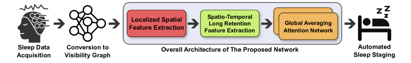
Figure 1: An overview of the proposed system. It begins with acquiring EEG data from the devices and converting it to visibility graphs. It is then passed to the model, and it captures all the relevant features of the data and estimates the sleep stage.

II Related Work

Various methodologies have been used to automatically detect sleep stages, utilizing traditional and machine learning techniques. Conventional methods encompass a variety of techniques, such as analysis of polysomnography data (PSG), electrodermal activity (EDA), and sleep depth information derived from EEG data. For example, visual analysis of PSG data, using multiple biosignals, has proven to be an effective tool for manual evaluation of sleep quality [17]. The application of PSG analysis involves the interpretation of specific signal patterns and characteristics that adhere to defined guidelines. In contrast, analysis of EDA patterns has been shown to identify specific characteristics correlated with sleep quality, thus facilitating the identification of sleep stages [18, 19]. EDA reflects variations in skin conductance due to sweating-related changes, which correspond to different sleep stages, as the EDA pattern fluctuates in tandem with sleep stage transitions. In addition, estimating sleep depth from EEG data and subsequently identifying relevant sleep stages has exhibited promising findings. For example, [20] introduced the Z-PLUS algorithm, which estimates sleep depth and classifies it into different sleep epochs such as light sleep, deep sleep, and rapid eye movement. However, these traditional methodologies have inherent limitations: they are often time-consuming, subjective, and financially burdensome [17]. Techniques involving visual analysis are particularly labor intensive and susceptible to human error, leading to inconsistencies in sleep stage classification [21]. Furthermore, they lack real-time detection capabilities, which requires post-processing and manual review prior to drawing conclusions, making them less suitable for clinical environments [22]. Traditional methods also struggle to capture the complexity of sleep dynamics, frequently overlooking subtle patterns and variations present in sleep data [23].

In contrast, machine learning techniques have demonstrated their potential for automatic, rapid, and precise sleep staging. They are also recognized for their ability to handle large volumes of data and derive intricate and meaningful representations from it [24]. [25] introduced an innovative framework for automated sleep staging using convolutional neural network (CNN), which simultaneously classifies sleep stages and predicts the epochs of adjacent labels. This method used dependencies among consecutive epochs to enhance accuracy. Their proposed model is also capable of making multiple decisions by applying ensemble-of-model techniques. Ultimately, the information is aggregated to produce a final prediction. Although their ensemble methods outperformed singleton methods, they often resulted in computational overhead. Furthermore, the model’s ability to generate multiple outputs based on probabilistic aggregation can diffuse the classification confidence, an undesirable trait in detection tasks. Similarly, [26] proposed an ensemble-based classifier that combines principal component analysis and rotational SVM to classify the five sleep stages. However, their model, which relies on single channel EEG data, does not exhibit channel-agnostic behavior. Additionally, using non-linear algorithms and principal component analysis simplifies the data’s complex behavior, leading to oversimplified decisions. [27] presented the Competitive Multiverse Optimization with a Deep Learning-based Stage Classification (CMVODL-SSC) model that uses EEG signals to classify sleep stages. This model incorporates data preprocessing and utilizes a cascaded long-short-term memory (CLSTM) model, using the CMVO algorithm for hyperparameter tuning. Nevertheless, the use of LSTM models, which maintain long-term data, incurs memory overhead, and the reliance on a single dataset restricts the model’s generalization. Furthermore, [28] introduced a unique framework for automatic sleep staging using CNN and cortical connectivity images. However, their cortical connectivity images encountered several problems. For example, the utilization of a general head anatomy model limits adaptability to individual participants and decreases localization accuracy, necessitating expert intervention. Moreover, the limited number of electrodes used to produce these images of cortical connectivity results in an ill-posed inverse problem, due to the mismatch between the number of electrodes and the numerous active sources in the cortex [29].

To summarize, an automated approach is required to determine sleep stages. It should choose features that effectively extract all pertinent information from the signals, capturing the complex dynamics intrinsic to these features. Furthermore, the method must be computationally efficient and versatile enough to classify different stages across multiple datasets or varying patterns.

III Materials and Methods

Figure 2: This illustration depicts the conversion process from the raw EDF data into time-series data. The process can be divided into three sections: filtering the desired channels, mapping the epoch data with the corresponding sleep stage, and converting to time-series data. Channels are chosen based on the commonness of a channel across the used datasets in the experiment. The epochs have to be of the same length before the time-series conversion.

III-A Construction of the Visibility Graph

A Visibility Graph (VG) is an algorithm that maps a series of data to a network graph [30]. This graph provides an insightful visual representation of time series data, capturing the intrinsic properties of the series. Generally, there are two types of VG: natural VG and horizontal VG. For the purpose of this paper, we focus on Natural VG. Figure 3 illustrates a sample undirected representation of a natural VG. In this graph, each vertex corresponds to a data point in the series, arranged in the same sequence as the series. The magnitudes of the vertices represent the actual values of the data points. The edges between vertices are drawn based on the visibility between the vertices and their neighboring vertices. Consider $s(t_{x})$ to be a univariate time series where $t_{x}$ denotes the time events defined as $\{0,1,2,\ldots N\}$ with $N$ being the total events. The construction of a VG involves creating $N$ vertices in the same order as $t_{x}$, with their magnitudes defined by the series values $s(t_{x})$.

Figure 3: Sample undirected natural VG with 10 vertices equivalent to 10 series data in an ordered manner. The horizontal axis refers to the data points, and the vertical axis refers to their magnitude. The straight lines refer to the links connecting the nodes in the graph, indicating a relationship between them.

Consider $t_{i}$ and $t_{j}$ as two random time events with corresponding vertices $s(t_{i})$ and $s(t_{j})$. The vertices will be mutually visible if there exists a vertex $s(t_{k})$ corresponding to the time event $t_{k}$ positioned between $s(t_{i})$ and $s(t_{j})$ such that $t_{i}<t_{k}<t_{j}$ and meets the following condition:

$$s(t_{k})<s(t_{j})+[s(t_{i})-s(t_{j})]\dfrac{t_{j}-t_{k}}{t_{j}-t_{i}}$$ (1)

In Equation 1, it is inferred that an edge between $s(t_{i})$ and $s(t_{j})$ will be established only if $s(t_{k})$ does not intersect the visibility line extending from $s(t_{i})$ to $s(t_{j})$, or equivalently, $s(t_{k})$ resides below the line joining $s(t_{i})$ and $s(t_{j})$.

III-B Generating the Force-directed Layout

[31] originally introduced the Force-directed layout (FDL) as an undirected graph influenced by the Spring model [32]. Consider a graph $G=\{V,E\}$ composed of a set of vertices $V$ and edges $E$. FDL aims to arrange the vertices $V$ in such a way that the overall spring energy of the system is minimal, with the spring energy representing the graph-theoretic distance (i.e., Euclidean geometric distance) between each pair of vertices in the set $V$.

Consider a set of particles $P=\{P_{1},P_{2},P_{3},\ldots,P_{n}\}$ corresponding to a series of vertices $V=\{V_{1},V_{2},V_{3},\ldots,V_{n}\}$, where $n$ denotes the total number of particles. Each particle $P_{ij}$ is interconnected through springs. The total energy of the system, indicative of its degree of imbalance, $E$, can be formulated as follows:

$$E=\sum_{i=1}^{n-1}\sum_{j=i+1}^{n}\dfrac{1}{2}k_{ij}{(\mid P_{i}-P_{j}\mid-\>l_{ij})}^{2}$$ (2)

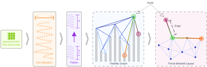
Figure 4: This illustration illustrates generating an FDL graph from time-series data. The conversion process can be divided into three steps: normalizing the data, constructing the visibility graph, and generating a force-directed layout. The FDL has been plotted utilizing the Kamada-Kawai layout algorithm.

In Equation 2, $l_{ij}$ represents the minimum desired length of the spring interconnecting $p_{i}$ and $p_{j}$. It is mathematically expressed as $l_{ij}=L\times d_{ij}$, where $L$ denotes the preferred length of an individual edge within the display plane, and $d_{ij}$ signifies the shortest path between the vertices $V_{i}$ and $V_{j}$. Furthermore, the parameter $k_{ij}$, indicative of the stiffness of the spring between $p_{i}$ and $p_{j}$, is delineated as $k_{ij}=\frac{K}{d_{ij}^{2}}$, where $K$ is a constant. The method for creating FDL from sleep data in European Data Format (EDF) is outlined in Algorithm 1.

1

Input: Raw EEG data in EDF format

Output: FDL graph images

Data: EDF file paths as list

$\mathcal{E}\leftarrow\emptyset$;

foreach $(edfPath,annotPath)$ in $\exists paths$ do

       $eeg\leftarrow readRawEdf(edfPath)$;

       $eeg^{\prime}\leftarrow crop(eeg,[0,\exists t])$;

       $eeg^{\prime}\leftarrow resample(eeg^{\prime},\exists f)$;

       $setAnnotation(eeg^{\prime},annotPath)$;

       $\mathcal{E}\leftarrow\mathcal{E}+eeg$;

      

end foreach

$\mathcal{H}\leftarrow\emptyset$;

foreach $eeg$ in $\mathcal{E}$ do

       $events\leftarrow eventsFromAnnotation(eeg)$;

       $epoch\leftarrow Epoch(eeg,events,\ldots)$;

       $\mathcal{H}\leftarrow\mathcal{H}+epoch$;

      

end foreach

$\mathcal{D}(X,Y)\leftarrow\emptyset:\{\mathbb{R},\mathbb{N}\}$;

foreach $epoch$ in $\mathcal{H}$ do

       $x\leftarrow getData(epoch)$;

       $y\leftarrow getEvent(epoch,[:,2])$;

       $\mathcal{D}\leftarrow\mathcal{D}+(x,y)$;

      

end foreach

$\mathcal{I}(X,Y)\leftarrow\emptyset:\{\mathbb{R},\mathbb{N}\}$;

foreach $(X,Y)$ in $\mathcal{D}$ do

       $nvg=NaturalVG()$;

       $vgTrain\leftarrow nvg(X)$;

       $img\leftarrow drawFdl(vgTrain)$;

       $\mathcal{I}\leftarrow\mathcal{I}+(img,Y)$;

      

end foreach

Algorithm 1 Generation of Force-directed Layout

III-C Proposed Methodology

III-C1 Convolutional Dilation

CNN is an architecture designed to adapt to multidimensional data invariances through local connection patterns with trainable kernels constrained by weights. Standard CNNs consist of three primary layer types: convolutional layers, pooling layers, and fully connected layers. The convolutional layer generates the neuron output for local input regions by calculating the dot product of their weights (obtained from the kernel) and the current local region where the convolution is applied. The pooling layer reduces the spatial dimensions of the output, thus reducing the number of parameters. The fully connected layer ultimately generates class scores through backpropagation. Dilated convolutions [33] are a crucial aspect of deep learning frameworks, allowing for the expansion of the receptive field filter without increasing the parameter count or computational load [34]. This is achieved by incorporating gaps or holes between the elements of the convolutional kernel, effectively adding zeros (padding) to it [35]. By adding these holes, dilated convolutions enable the filters to gather information from a larger context while preserving the input’s spatial resolution. The dilation rate, which dictates the gaps between the elements of the kernel, controls the degree of expansion of the receptive field [36]. By employing dilated convolutions, models can effectively blend local and contextual information, capturing long-range dependencies and contextual details, thereby enhancing their feature extraction capabilities across various scales and boosting performance in tasks like semantic segmentation and object detection.

III-C2 Multihead Self Attention

An attention function is a process of mapping a query $Q$ and a set of key-value ($K-V$) pairs to an output, where the query, keys, values, and output are all vectors [37]. The output is computed as a weighted sum of the values, where a compatibility function of the query with the corresponding key computes the weight assigned to each value. Scaled dot-product attention is a member of the dot-product attention family, where the attention score is calculated using dot matrix multiplication of the input vectors. To avoid vanishing-gradient problems, the result of the dot product is scaled by a factor of $\sqrt{d_{k}}$ where $d_{k}$ is the dimension of the key vector. This way of scaling the dot-product is called the scaled dot-product attention mechanism.

$$\text{Attention }(Q,K,V)=\text{softmax}(\dfrac{QK^{T}}{\sqrt{d_{k}}})V$$

Unlike single-head attention, multi-head attention, as shown in Figure 5, linearly projects queries, keys, and values h times with different learned linear projections to different dimensions, respectively. It transforms input queries, keys, and values into multiple subspaces using different learnable projection matrices. Each subspace is then used to compute the attention weights independently, allowing the model to focus on different aspects of the input data. The outputs from these multiple attention heads are concatenated and transformed by a final linear layer to produce the final output.

$$\text{Multi-head}(Q,K,V) =\text{concat}(\text{head}_{1},\ldots,\text{head}_{h})W^{o}$$ (3)

$$\text{where head}_{i} =\text{Att}(QW_{i}^{Q},KW_{i}^{K},VW_{i}^{V})$$

$$\text{where Att}(Q,K,V) =\text{Attention}(Q,K,V)$$

In this context, the projections are delineated by the parameter matrices:

$$W_{i}^{Q} \in\mathbb{R}^{d_{model}\times d_{k}} W_{i}^{K} \in\mathbb{R}^{d_{model}\times d_{k}}$$

$$W_{i}^{V} \in\mathbb{R}^{d_{model}\times d_{v}} W^{O} \in\mathbb{R}^{hd_{v}\times d_{model}}$$

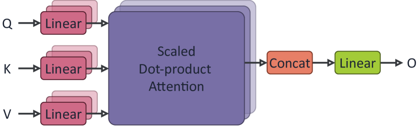
Figure 5: Multihead attention network composed of multiple attention layers operating concurrently. Each attention layer comprises a query vector $Q$, a key vector $K$, a value vector $V$, and an output vector $O$.

III-C3 Network Architecture

We present our proposed architecture, as shown in Figure 6, designed for automatic scoring of sleep stages. This comprehensive network encompasses three distinct components: the Localized Spatial Feature Extraction Network (LSFE), the Spatio-Temporal-Temporal Long Retention Network (S2TLR) and the Global Averaging Attention Network (G2A). Each component generates a unique set of feature maps denoted as $\mathcal{F}_{n}$, where $n$ represents the total number of feature maps. The subsequent sections provide an in-depth discussion of each component.

Figure 6: The illustration of the proposed model architecture. The network is composed of three distinct blocks: LSFE, S2TLR, and G2A. LSFE extracts information based on the local features, whereas S2TLR extracts meaningful and computationally efficient data from the retained long information stack. Finally, G2A averages the attention weights and concludes with a sleep stage.

Localized Spatial Feature Extraction Network (LSFE)

As the initial compositor of our proposed network, it adeptly captures the local characteristics of the FDL images. Let $\mathcal{I}$ represent the training set of size $S$, defined as $\{\mathcal{I}_{s}\}^{S}_{s=1}$. Each input, $\mathcal{I}_{i}$, is characterized as $\mathcal{I}_{i}=\{x_{i},y_{i}\}$, where $x_{i}$ denotes the FDL image tensor of dimensions $(128,128)$, i.e., $x=\{x_{128}\times x_{128}\}$. The variable $y_{i}$ corresponds to the annotated sleep stage of the respective FDL data $x_{i}$. To encapsulate the local features of the FDL image, the compositor develops the structure designated as LSFE-CNN, which is composed of two standard CNN layers, two dilated CNN layers, a single flatten layer, and two fully connected layers. The aggregation of these layers forms the initial feature map $\mathcal{F}_{1}$, which encapsulates all the local variations in the data. Four maximum pooling layers succeed the four CNNs. For the standard CNNs, each possesses a configuration $\{H,W,C\}$ where $(H,W)\equiv(2,2)$ indicates the kernel size, and $C$ denotes the number of kernels, being 16 and 32 for the first two CNNs respectively. The conventional CNNs traverse the entire FDL graph with a receptive field window of size $[2,2]$ and extract the most pertinent information using a maximum-pool strategy, determined by the formula: $max(0,p)$ where $p$ represents the scanning data point. In contrast, for the dilated CNNs, each is configured with $\{H,W,D,C\}$ where $(H,W)\equiv(2,2)$ is the kernel size, $D=2$ is the dilation rate and $C=64\text{ and }128$ are the number of kernels, respectively. Similarly to the conventional CNNs, the dilated CNNs also employ the maximum-pool strategy. However, unlike the conventional methods, the size of the receptive field can be adjusted by a factor of $l$, as delineated below:

$$(F\ast\!_{l}\;k)(p)=\sum_{s+lt=p}F(s)\;k(t)$$

In this study, we consider $F:\mathbb{Z}^{2}\rightarrow\mathbb{R}$ as a discrete function and $k:\Omega_{r}\rightarrow\mathbb{R}$ as a discrete filter size where $\Omega_{r}=[-r,r]^{2}\cap\mathbb{Z}^{2}$ [33]. Our proposed architecture employs a dilation rate of $l=2$, effectively skipping one data point along each dimension. This facilitates the capture of an expanded range of data with computational requirements comparable to those of conventional CNNs, thereby expediting the detection of salient features. Following each CNN layer, the rectified linear unit (ReLU) activation function is used to address the vanishing gradient problem. Subsequently, two fully connected networks are deployed, comprising 256 and 128 neural units, respectively, followed by a flatten layer. To prevent overfitting, a dropout layer with a rate of 0.5 is incorporated into the final layer of this network.

Spatio-Temporal-Temporal Long Retention Network (S2TLR)

The purpose of this compositor is to encapsulate the most pertinent information within an extended temporal event-data structure. The feature map $\mathcal{F}_{2}$ consists of two instances of the reshaped local features derived from the LSFE network, sequentially processed through the multi-head attention (MHA) network. Through convolution via the LSFE network, we obtain the most critical spatial features, which are then input into the S2TLR network. Let $\mathcal{I}_{S2TLR}$ represent the input data to the S2TLR network, characterized by the dimensions $(b,1,128)$, where $b$ is the batch size. In our experiments, we utilized batch sizes of $b=\{32,64,128,256,512,1024\}$. The input data $\mathcal{I}_{ST}$ is configured as $(\mathcal{I}_{ST},\mathcal{I}_{ST})$ and fed into the MHA with $h=3$ heads to compute the temporal relationships among the spatial features, referred to as self-attention weights. We denote this attention as $\mathcal{A}_{ST}=Att(\mathcal{I}_{ST},\mathcal{I}_{ST})$, as shown in Equation 3. This configuration, designated as S2TLR-MHA, implies the spatio-temporal interaction of the convolved features from the LSFE network. The $\mathcal{A}_{ST}$ output is subsequently embedded in another MHA network, producing data referred to as $\mathcal{I}_{TT}$, which symbolizes the temporal-temporal relationship of the spatio-temporal features. The data $\mathcal{I}_{TT}$ is processed in the configuration $(\mathcal{I}_{TT},\mathcal{I}_{TT})$ through the network with the same number of heads as $\mathcal{A}_{ST}$, and this attention is referred to as $\mathcal{A}_{TT}=Att(\mathcal{I}_{TT},\mathcal{I}_{TT})$. This represents the S2TLR-DMHA block depicted in Figure 6, thereby completing the spatial-temporal-temporal computational pipeline.

Global Averaging Attention Network (G2A)

The G2A network equilibrates the weights between the localized weights, denoted as $W_{l}$, and the global attention weights, denoted as $W_{g}$, which represent the feature map $\mathcal{F}_{3}$. This network achieves a reduction in computational overhead by half through the process of averaging both local and global weights. This approach facilitates the optimization and equilibrium of the resultant attention. The optimized average is consequently expressed as follows:

$$W_{o}=Avg(W_{l},W_{g})=\dfrac{W_{l}^{(1,128)}+W_{g}^{(1,128)}}{2}$$

In this context, $W_{o}$ represents the optimized weight, maintaining the identical data dimensionality as $W_{l}$ and $W_{g}$, specifically $(1,128)$. The local weight $W_{l}$ corresponds to the attention weights from the $\mathcal{A}_{ST}$ block, which encompasses the S2TLR-MHA features, whereas the global weight $W_{g}$ pertains to the attention weights from the $\mathcal{A}_{TT}$ block, incorporating the S2TLR-DMHA features. $W_{o}$ enables a balanced attention mechanism by combining the changes in spatial dimension captured by S2TLR-MHA and the temporal retention of these features of S2TLR-MHA throughout an entire epoch, as captured by S2TLR-DMHA. Subsequently, $W_{o}$ is flattened and passed through a sequence of four fully connected (FC) layers with neural units of $\{512,128,64,32\}$, respectively, to yield the final output, which consists of scoring the targeted sleep stage. This is accomplished by channeling the data through a final FC layer with a neural unit of $n$, denoting the number of sleep stages in the specific dataset.

IV Experimental Setup

IV-A Dataset Description

We applied our proposed model to three distinct and publicly available datasets to evaluate its performance. One of these datasets is frequently utilized in the existing literature, so we included it in our study as a benchmark dataset. The remaining datasets were used to assess the robustness of our model due to their varying signal characteristics. The details of the three datasets are provided in the subsequent sections.

IV-A1 EDFX

The Sleep EDFX dataset [38] from PhysioNet comprises two subsets: the Sleep Cassette (SC) study and the Sleep Telemetry (ST) study, with a total of 197 whole-night polysomnographic (PSG) sleep recordings including EEG, electroocoulogram (EOG), chin electromyography (EMG), and event markers. The first subset studies the impact of aging on sleep and includes 153 SC* files with patients aged 25 to 101 years. The second subset analyzes the effects of temazepam on sleep and contains 44 ST* files from 22 unique subjects. The EOG and EEG signals were acquired with a sampling frequency of 100 Hz. For the purposes of our study, we selected the Fpz-Cz channel to ease the automated sleep analysis process. The *PSG files encompass the whole-night’s sleep recordings, while the *Hypnogram files provide annotations of sleep patterns including stages W, R, 1, 2, 3, 4, M (movement time), and ? (not scored). Among these eight classifications, stage M was not considered in our study. The remaining sleep stages are included and their distribution is shown in Figure LABEL:fig_class_dist(a).

Ref	Dataset	EEG Channel	Sampling Rate	Size1	#Sample	#Class
[38]	EDFX	Fpz-Cz	100 Hz	434 MB	25000	7
[39, 40]	HMC	C3-M2		487 MB		5
[41, 42]	NCH			469 MB		6

• The size is not of the actual dataset in the EDF format. It is the size of the FDL graphs converted from the EDF format.

TABLE I: Properties of the three used datasets.

IV-A2 HMC

The Haaglanden Medisch Centrum sleep staging dataset [41, 42] consists of 151 full-night PSG sleep recordings collected from a diverse group of individuals referred for PSG examination at the Haaglanden Medisch Centrum (HMC, The Netherlands) sleep center. The dataset comprises recordings from 85 male and 66 female patients, with an average age of 53.9 ± 15.4, covering a variety of sleep disorders. The PSG recordings include EEG, EOG, chin EMG, and ECG activity, plus event annotations for sleep stage scoring carried out by HMC sleep technicians. The PSG data include EEG from four channels: F4-M1, C4-M1, O2-M1, and C3-M2, along with other EOG, EMG, and ECG channel data. However, for our study, we focused only on the C3-M2 channel for sleep analysis. Although originally recorded at 256 Hz, the data was resampled to 100 Hz for consistency. The class distribution for each stage in the HMC dataset is presented in Figure LABEL:fig_class_dist(b).

IV-A3 NCH

The Sleep DataBank from Nationwide Children’s Hospital (NCH) [39, 40] is an extensive dataset comprising 3,984 pediatric sleep studies performed on 3,673 distinct patients at NCH in the USA. This dataset contains longitudinal clinical data sourced from the Electronic Health Record (EHR), which includes information on encounters, medications, measurements, diagnoses, and procedures, as well as published polysomnography (PSG) data with physiological signals. The unique aspects of this dataset are its significant size, its specific focus on pediatric patients, the real-world clinical environment, and the comprehensive clinical data. For our model, we used the C3-M2 EEG channel to classify sleep stages. Figure LABEL:fig_class_dist(c) displays the distribution of sleep stages within the NCH databank.

IV-B Handling Data Imbalance

Datasets frequently demonstrate notable class imbalance, with a substantial skew towards one particular class. This imbalance tends to cause network overfitting and bias towards the prevalent class, which is not ideal. To tackle this issue, we can either down-sample or over-sample the data. Down-sampling may not be effective if other classes have too few samples, as the network would lack sufficient data to learn from. Thus, using the oversampling technique is more beneficial in generating synthetic data that resemble the original data, ensuring that each class has an equal number of samples. In our methodology, we have used the synthetic minority sampling technique (SMOTE) [43], a widely used approach to handle unbalanced datasets. This technique generates synthetic instances for the underrepresented class to balance the class distribution. SMOTE creates new synthetic instances by interpolating between existing instances of the minority class. The algorithm selects a minority instance and identifies its k nearest neighbors in the feature space based on the oversampling requirement. A new synthetic instance is created by randomly choosing one of these neighbors and generating an example along the line connecting the chosen neighbor and the original minority instance.

IV-C Training Strategy

To achieve optimal model performance, it is essential to first balance the data accurately and then strategically divide them for training and testing. The overall procress of training the proposed network and automatic sleep staging has been described in Algorithm 2. In our experiments, we used a random seed value of 13 to ensure reproducibility. Model training involved a 10-fold stratified cross-validation across all datasets. We split the datasets into training and testing sets with an 80:20 ratio to evaluate the model’s performance on new, unseen data. The model was trained using sparse categorical cross entropy as the loss function. Training was carried out over 200 epochs using the Adam Optimizer with a learning rate of 0.001. During training, an early stopping mechanism was used with a patience threshold of 15, monitoring validation accuracy in maximum mode.

1

Input: Force-directed Layout data

Output: Model’s prediction

Data: Network graphs as image files

$\mathcal{I}\leftarrow\emptyset$ // empty list;

foreach $path$ in $paths$ do

       $img\leftarrow loadImgAsArray(path)$;

       $\mathcal{I}\leftarrow\mathcal{I}\mid\mid img$ // append to the list;

      

end foreach

$labelPath\leftarrow\;^{\prime\prime}\ldots label.csv^{\prime\prime}$;

$\mathcal{Y}\leftarrow loadLabelsFromCsv(labelPath)\in\mathbb{W}$;

$\mathcal{I}\leftarrow N(\mathcal{I})$ // normalize;

$(\tilde{\mathcal{I}},\tilde{\mathcal{Y}})\leftarrow smote(\mathcal{I},\mathcal{Y})$ ;

$k\leftarrow 10$ ;

$\mathcal{F}\leftarrow skf(k,\tilde{\mathcal{I}},\tilde{\mathcal{Y}})$ // stratified k-fold ;

$\mathcal{M}\leftarrow AttDiCNN(\ldots)$;

$modelTrain(\mathcal{M},\mathcal{F},\ldots,\tilde{\mathcal{I}},\tilde{\mathcal{Y}})$;

$\mathcal{P}\leftarrow\mathcal{M}(\mathcal{I})\in\mathbb{W}$ // model’s prediction;

Algorithm 2 Proposed Workflow

V Results and Discussions

V-A Evaluation Metrics

A comprehensive set of evaluation metrics was employed to assess our model’s performance, encompassing accuracy (Acc), top-k accuracy, Cohen’s kappa coefficient $\kappa$ [44], area under the curve (AUC), precision, recall, and the macro F1 score. Additionally, to elucidate the model’s error rate in predicting sleep stages, we incorporated two error metrics: mean absolute error (MAE) and mean squared error (MSE). Accuracy, as delineated in Equation 4, quantifies the proportion of correctly classified instances. Analogous to the accuracy metric, the top-k accuracy score, articulated in Equation 5, posits that a prediction ($\hat{y}$) is deemed correct if it is among the top $k$ highest predicted values.

$$Acc(y,\hat{y})=\dfrac{1}{N}\sum_{i=0}^{N-1}1\left(\hat{y_{i}}=y_{i}\right)$$ (4)

$$Top-k\;Acc(y,\hat{y})=\dfrac{1}{N}\sum_{i=0}^{N-1}\sum_{j=1}^{K}1\left(\hat{y}_{i,j}=y_{i}\right)$$ (5)

$$Precision=\dfrac{TP}{TP+FP}$$ (6)

$$Recall=\dfrac{TP}{TP+FN}$$ (7)

$$F1=\dfrac{2\times Precision\times Recall}{Precision+Recall}$$ (8)

$$MAE=\dfrac{1}{N}\sum_{i=0}^{N-1}|y_{i}-\hat{y_{i}}|$$ (9)

$$MSE=\dfrac{1}{N}\sum_{i=0}^{N-1}\left(y_{i}-\hat{y_{i}}\right)^{2}$$ (10)

In this context, $N$ represents the total number of samples, with $y$ as the actual value and $\hat{y}$ as the predicted value for the $i$th instance. $K$ denotes the maximum number of predictions defined in the top-k accuracy scenario. $TP$, $FP$, and $FN$ stand for true positive, false positive, and false negative, respectively. In Equation 4, $1(x)$ denotes the 0-1 indicator function, yielding $1$ if $y$ matches $\hat{y}$ and $0$ otherwise. Conversely, in Equation 5, $1(x)_{\mathbb{A}}$ represents the 0-1 indicator function, returning $1$ if $x$ belongs to $\mathbb{A}$ and $0$ otherwise.

V-B Performance Evaluation

We used two different evaluation methodologies, namely, intraperformance and interperformance comparisons, to rigorously assess the effectiveness of our model. Within the intra-performance framework, we delineated the performance variations across various iterations of our model. Conversely, the inter-performance framework enabled us to compare our model’s performance against established findings in the existing literature, thereby demonstrating its preeminence.

V-B1 Intra Performance

In this section, we evaluate our proposed model’s performance by altering the batch sizes to observe how the model behaves with different amounts of data processed simultaneously.

TABLE II: Model performance with different parameters.

Dataset	Batch Size	Parameters
		Acc.	Top-2 Acc.	Top-3 Acc.	Kappa $\kappa$	AUC	Precision	Recall	MF1	MAE	MSE
EDFX	32	0.8456	0.9780	0.9928	0.8043	0.9401	0.8995	0.9095	0.9028	0.2700	0.8995
	64	0.9184	0.9866	0.9950	0.8919	0.9666	0.9181	0.9491	0.9316	0.1460	0.6239
	128	0.9708	0.9966	0.9982	0.9629	0.9884	0.9760	0.9822	0.9787	0.0528	0.3883
	256	0.9778	0.9964	0.9976	0.9718	0.9892	0.9793	0.9824	0.9807	0.0626	0.4917
	512	0.9712	0.9952	0.9980	0.9635	0.9892	0.9754	0.9835	0.9793	0.0594	0.4443
	1024	0.9856	0.9982	0.9992	0.9817	0.9932	0.9863	0.9890	0.9877	0.0354	0.3541
HMC	32	0.3866	0.5706	0.7282	0.0415	0.5171	0.7248	0.2272	0.1629	1.0952	1.5436
	64	0.5900	0.7370	0.8440	0.4009	0.6787	0.8405	0.4852	0.5417	0.7166	1.2467
	128	0.9940	0.9988	1.0000	0.9921	0.9971	0.9930	0.9956	0.9943	0.0142	0.1934
	256	0.9892	0.9994	1.0000	0.9858	0.9927	0.9872	0.9880	0.9875	0.0212	0.2154
	512	0.9918	0.9998	1.0000	0.9892	0.9947	0.9917	0.9915	0.9915	0.0120	0.1470
	1024	0.9966	0.9998	1.0000	0.9955	0.9977	0.9960	0.9962	0.9961	0.0086	0.1556
NCH	32	0.9780	0.9972	0.9996	0.9671	0.9904	0.9860	0.9859	0.9857	0.0248	0.1744
	64	0.9702	0.9964	0.9996	0.9556	0.9880	0.9678	0.9824	0.9744	0.0356	0.2209
	128	0.9908	0.9972	0.9996	0.9862	0.9947	0.9939	0.9914	0.9926	0.0136	0.1497
	256	0.9732	0.9966	0.9996	0.9599	0.9888	0.9835	0.9838	0.9833	0.0324	0.2088
	512	0.9866	0.9974	0.9996	0.9799	0.9933	0.9913	0.9896	0.9903	0.0160	0.1456
	1024	0.9794	0.9972	0.9996	0.9692	0.9908	0.9877	0.9865	0.9870	0.0284	0.2098
Minimum		0.3866	0.5706	0.7282	0.0415	0.5171	0.7248	0.2272	0.1629	0.0086	0.1456
Maximum		0.9966	0.9998	1.0000	0.9955	0.9977	0.9960	0.9962	0.9961	1.0952	0.2209
Average		0.9164	0.9577	0.9750	0.8777	0.9439	0.9543	0.9111	0.9082	0.1469	0.4340

As previously mentioned, we conducted tests using three distinct datasets. Batch sizes ranged from 32 to 1024 for each dataset, and the model’s performance exhibited variations with these changes, which are detailed below.

In the case of the EDFX dataset from Table II, we can see that we have a minimum accuracy of 84.56% and a maximum accuracy of 98.56%. This implies that our proposed model correctly predicted the sleep stages at least 84.56% of the time in total instances. It also means that our model could not correctly predict 1.44% of the time even when it performed the best classifying of the sleep stages. However, the difference in incorrectly classifying the stages is reduced in the case of top-2 and top-3 accuracy with a maximum staging rate of 99.82% and 99.92%. This implies that even if the model failed to predict in the first instance, it predicted almost perfectly almost all the time at its second and third instances. In Figure 7, it is visible that the model continued to improve its prediction capability when the number of epochs increased. The model seems to learn very smoothly in its training phase. However, it always struggled to predict the validation set and had a scattered outcome, which slowly submerged and became very smooth at the end. In the case of error reduction, the MAE remained smooth almost all the time and improved slowly as the batch sizes grew larger. However, MSE seems to be very large in number in smaller batch sizes and improves with time. The MSE’s large values are due to their higher sensitivity because of their squared nature. Our proposed model had an MAE of 0.0354 and an MSE of 0.3541 in our largest batch size of 1024.

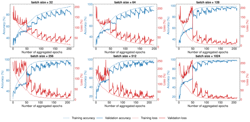
Figure 7: Performance metrics (accuracy and loss) plotted over epochs during training and validation for the EDFX dataset, using batch sizes of 32, 64, 128, 256, 512, and 1024.

However, Table II shows a clear contrast in performance between the EDFX and HMC datasets, especially at the initial stages. The HMC dataset performed very poorly, with a batch size of 32. Initially, it had an accuracy of only 38.66%. However, it converged faster, starting from a batch size of 128, and it is slightly higher than the performance of the EDFX dataset for the same batch size and soon after, it outperformed the EDFX model’s performance. The superiority is also noticeable in the case of top-2 and top-3 accuracy, particularly for the top-k performance, it predicted ideally starting from the batch size of 128 onward. There is also a visible difference in the reduction of false prediction: the model’s error rate. The HMC’s model performed very well in the error metrics for the same batch size compared to the EDFX’s. For the HMC dataset, we have a minimum error of 0.0086 and 0.1556 for MAE and MSE, respectively. It is evident from Figure LABEL:fig_hmc_train_val_curve that in the case of the training phase, both accuracy and error seem to converge in the intended direction very smoothly. However, like in the case of the EDFX dataset, the model struggled to stabilize itself and had quite a scattered performance over the whole epochs. The model tends to stabilize better as the number of batch sizes increases in the case of accuracy and error metrics, except for a large spike approximately at 50 epochs, starting from the batch size of 128.

The NCH dataset’s model performed better consistently from the beginning compared to the EDFX and the HMC datasets. However, one interesting pattern to note here is that, unlike the cases of EDFX and HMC, where larger batch sizes positively impacted the model’s performance, the NCH dataset did not perform best for the largest batch size. In the case of NCH, the model performed best with a batch size of 128, achieving an accuracy of 99.08%, while with a batch size of 1024, it had an accuracy of 97.94%. Although for the top-2 accuracy, the performance varied, in the case of the top-3 accuracy, the performance was consistent with an accuracy of 99.96%. In the case of error rate, it outperformed the performances of the other two datasets, both in MAE and MSE, with the lowest values of 0.0136 and 0.1456, respectively. However, similar to the other two datasets, it has a smooth learning curve for both accuracy and loss values in training, and there are abrupt changes in the validation phases, slowly converging to their intended values as shown in Figure LABEL:fig_nch_train_val_curve.

Cohen’s kappa is used to quantify the reliability between two raters on an agreement. If we look at the $\kappa$ values in Table II, there are only four instances below the value of 0.90. According to Cohen’s kappa interpretation [45], a $\kappa$ value of 0.9 or greater implies an almost perfect level of agreement with around 82-100% of reliable data. So, according to statistics, our model predicted almost perfectly, and if two different versions of our model predicted new random data, they would agree in most cases. Some exceptions occurred for several batch sizes in the EDFX and HMC datasets. For example, although in the EDFX dataset, there is a strong level of agreement with 64-81% reliable data, in the case of the first two batch sizes of the HMC dataset, there is none and a weak level of agreement. It indicates that if two instances of the former models try to predict a sleep stage, almost every time, they will contradict each other. The rest of our model performance parameters, including precision, recall, and MF1, are detailed in Table II. In Figures LABEL:fig_mean_max_inter and LABEL:fig_mean_max_intra, we have also shown the mean and max performance of our model based on the inter-datasets and inter-batch size settings.

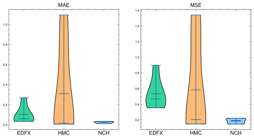
Figure 8: Representation of two error metrics for our model’s performance across different batch sizes for the three datasets.

Figure 8 illustrates the overall loss of the model based on three datasets for all the batch sizes. It is pretty noticeable that the NCH dataset performed very well with very little and minimized loss compared to the EDFX dataset. However, HMC had the highest error percentage among the three datasets, with an approximate median of 0.3. An interesting pattern to note is that, although the NCH had the lowest error, the plot width increased as the batch sizes indicated that our model performed the worst, which is not the case for EDFX and HMC. Their loss reduced with increasing batch sizes.

Overall, the model was able to correctly stage the sleep data automatically most of the time. Although there were significant fluctuations during the earlier epochs, it became more stable later on, and the validation performance was closely aligned with the training performance. The loss of the proposed function was consistently minimal, indicating good performance and preventing misdiagnosis.

Dataset	Ref.	Classifier	EEG Channel	#Param	Recall	Precision	MF1	Kappa $\kappa$	Accuracy
EDF/EDFX	[46]	4s-SleepGCN	Fpz-Cz	2.50 M	90.00	88.70	89.10	0.89	92.30
	[47]	CNN+Attention	Fpz-Cz	–	–	–	79.00	0.78	84.30
			Pz-Oz	–	–	–	74.10	0.74	80.70
	[48]	ADAST	Fpz-Cz	–	–	–	60.39	–	74.00
	[49]	AttnSleep	Fpz-Cz	–	–	–	78.10	0.79	84.40
	[50]	ST-GCN	Fpz-Cz Pz-Oz	–	90.90	87.40	89.00	0.88	91.00
	[9]	CNN+Attention	Fpz-Cz	–	–	–	84.50	–	93.70
	[51]	LS-SVM	Fpz-Cz Pz-Oz	–	96.50	–	–	0.87	97.40
	[52]	Genetic Algorithm	Fpz-Cz	–	91.19	–	–	0.92	92.41
			Pz-Oz	–	93.26	–	–	0.93	93.75
	[53]	CSCNN-HMM	Fpz-Cz	–	–	–	–	0.79	84.60
			Pz-Oz	–	–	–	–	0.76	82.30
	[54]	EEGSNet	Fpz-Cz	–	–	–	77.26	0.77	83.02
	[55]	RF-LGB	Fpz-Cz	–	–	–	92.001	0.864	91.20
			Pz-Oz	–	–	–	92.001	0.872	91.80
	[56]	TLCNN-DF	Fpz-Cz Pz-Oz	–	–	85.462	81.802	0.90	93.16
	Ours	AttDiCNN	Fpz-Cz	1.41 M	98.90	98.63	98.77	0.98	98.56
HMC	[57]	Generative Model	–	–	–	–	74.003	–	77.703
	[58]	DNN	–	–	–	–	–	0.70	77.00
	Ours	AttDiCNN	C3-M2	1.41 M	99.62	99.60	99.61	0.99	99.66
NCH	[59]	Transformer Model	–	–	–	–	70.50	0.71	78.20
	Ours	AttDiCNN	C3-M2	1.41 M	99.14	99.39	99.26	0.99	99.08

• No macro F1 was reported. Thus, a weighted F1 has been provided.

• The values were derived by calculating the average of each individual sleep stage.

• The values are based on the EOG data instead of the EEG data.

TABLE III: Model’s performance comparison with existing literature.

V-B2 Inter Performance

In the previous section, we discussed how our model performed with various batch sizes. In this section, we will evaluate our model’s performance in relation to existing studies.

Although we utilized three datasets to assess our model’s performance, to the best of our knowledge, the majority of existing literature primarily employs EDF or EDFX datasets, with some papers using HMC or NCH datasets. Most of the models in these studies have designed their architectures based on convolutional networks. For example, [56] introduced the TLCNN-DF framework, achieving an accuracy of 93.16% and a kappa of 0.90, indicating a perfect level of agreement. Their framework integrates information from two data sources: EEG and EOG. However, it may not always be practical to obtain both EEG and EOG data simultaneously from the same source. In addition, models that rely on transfer learning introduce computational complexity. [54] developed EEGSNet, a multilayer CNN that automatically classifies sleep scores from EEG spectrograms. They also utilized a bidirectional long-short-term memory model to capture transitional information from the extracted features. However, the retention of long-term memory throughout the model’s lifetime results in redundant information. Moreover, their model did not perform satisfactorily compared to state-of-the-art results. On the other hand, [51] proposed a cluster-based approach for robust sleep staging, outperforming numerous CNN-based methods, with an accuracy of 97.40% and a recall of 96.50%, which demonstrates strong model agreement. Furthermore, [52] adopted an ensemble method that utilizes genetic algorithms to classify sleep stages based on Fourier transformation. They evaluated their model’s performance on two distinct EEG channels: Fpz-Cz and Pz-Oz, achieving accuracies of 92.41% and 93.75%, respectively. Multiple authors have explored the incorporation of attention networks in deep learning layers to enhance overall model performance. For instance, [49] introduced AttnSleep, which employs a temporal context encoder with a multi-head attention mechanism to classify sleep stages. To extract meaningful features more effectively, they proposed multiresolution CNN and adaptive feature recalibration modules. The CNN network captures high- and low-frequency features, while the adaptive calibration module improves the quality of the features by modeling their interdependencies. Generally, they reported an overall accuracy of 84.40% and an MF1 score of 78.10, indicating a balanced performance between precision and recall. Similarly, [47] and [9] both utilized attention mechanisms alongside convolutional networks but observed significant performance variations of approximately 9-13%. [9] designed a CNN-based network to capture the characteristics of local EEG data, passing them to the attention network for better analysis of inter- and intra-epoch features. They achieved an overall accuracy of 93.70% and an MF1 of 84.50 for the Fpz-Cz channel. In contrast, [47] achieved overall accuracies of 84.30% and 80.70% for the Fpz-Cz and Pz-Oz channels, respectively, by decomposing input EEG signals into different frequency bands and feeding them to CNN and MHA networks. As illustrated in Table III, our proposed model exceeds the performance of state-of-the-art networks in all evaluation metrics, with significant differences and reduced computational complexity.

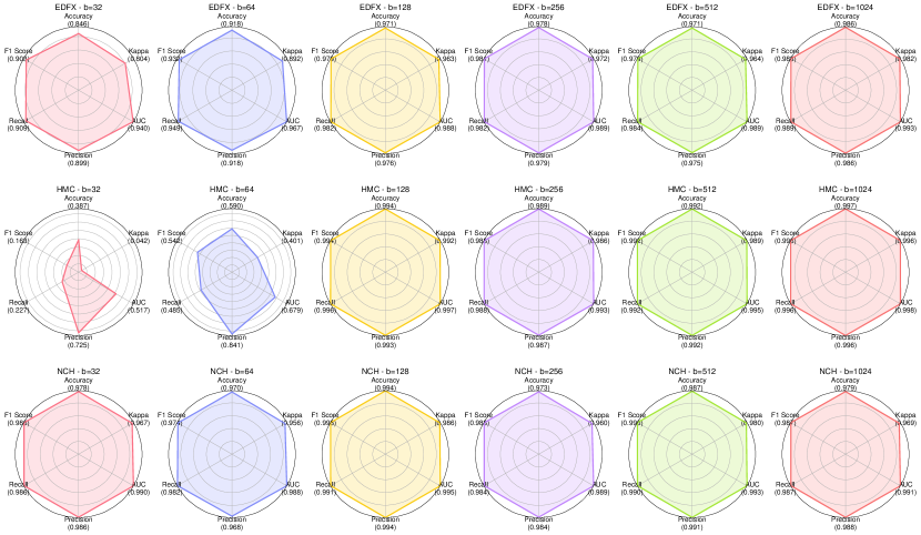
Figure 9: Reliability diagram of the model for the three datasets with batch sizes ranging from 32 to 1024, including six statistical metrics: accuracy, kappa, AUC, precision, recall, and F1 score.

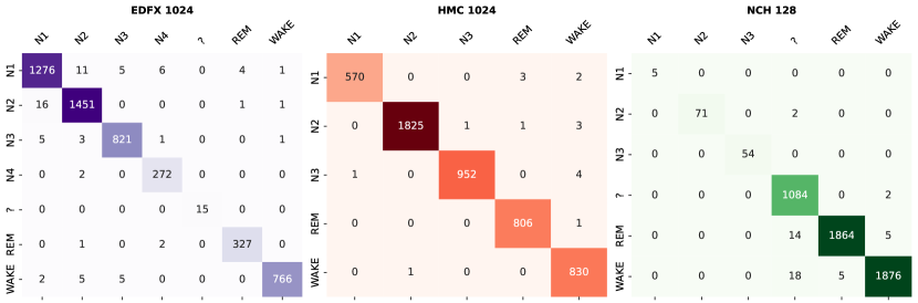
Figure 10: Confusion matrix displaying the leading three models with batch sizes of 1024, 1024, and 128 for their respective datasets.

V-C Inspecting Performance Robustness

Establishing a model’s robustness in conjunction with its performance efficacy is essential to affirm the reliability of the proposed methodology. Our model demonstrated commendable performance across all utilized datasets. As illustrated in Figure 10, the model accurately predicted nearly all sleep stages. For the EDFX dataset with a batch size of 1024, the N1 sleep stage exhibited the highest misclassification rate, with 27 instances. N1 was predominantly confused with the N2 stage in 11 out of 5000 samples. In contrast, the N2 class showed 18 misclassification cases, with 16 instances overlapping with the N1 sleep stage. Additionally, there were minor overlaps between the wake stage and the N2 and N3 stages. The model distinctly identified the remaining stages. Concerning the HMC dataset, also with a batch size of 1024, unlike the EDFX dataset, the model effectively resolved the confusion between the N1 and N2 stages, presenting zero overlap. However, some ambiguity was noted between the N2 and N3 sleep stages and the wake stage, with three and four overlapping instances, respectively. Furthermore, the model nearly perfectly classified the other stages. Similarly, for the NCH dataset with a batch size of 128, the model successfully ameliorated the N1 and N2 confusion, akin to the HMC dataset. Yet, a notable discrepancy was observed in the unknown (?) stage, which overlapped with the REM and wake stages in 14 and 18 instances, respectively.

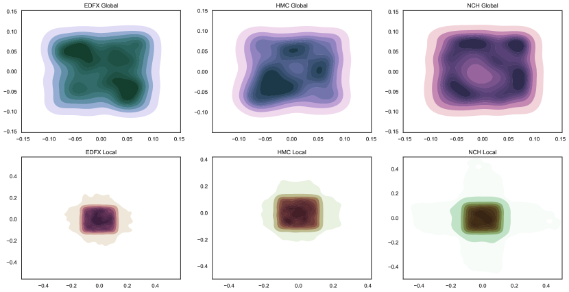
Figure 11: Kernel weight distribution comparison between the G2A module and the LSFE module to assess computational overhead.

In brief, out of 5000 test samples, the top-performing models successfully predicted 4928, 4983, and 4954 sleep stages for the EDFX-1024, HMC-1024, and NCH-128 datasets, respectively. Despite achieving accuracies of 98.56%, 99.66%, and 99.08% for each dataset, an observable trend is that performance decreases as the number of total sleep stages increases. To address this issue, careful feature engineering of the datasets is necessary, ensuring consistent signal properties, such as sampling frequency, channel data, or electrode usage, in addition to other parameters. The performance of the remaining batch sizes for the three datasets based on confusion matrix are shown in the Figure LABEL:fig_rest_cf. However, disregarding the error rates of 1.44%, 0.34%, and 0.92% for datasets with seven, five, and six sleep stages, respectively, the model’s consistent performance across all datasets suggests its viability as an automatic sleep staging tool.

To further evaluate the model’s robustness, we illustrated a reliability diagram as depicted in Figure 9. The underlying idea of the reliability diagram is that a larger diagram area implies a more reliable model. The six parameters included in this diagram are accuracy, kappa, AUC, precision, recall, and F1 score. Since higher values of these parameters denote better performance in their respective criteria, larger values result in a greater area, indicating a superior model. This setup allows us to visualize performance across datasets of the same batch size and across different batch sizes of the same datasets. In the EDFX dataset, it is clear that the model generally performed consistently, accurately classifying sleep stages, except for the model with a batch size of 32 which covered a smaller area in the performance metrics. The NCH model displayed an almost perfect area across all batch sizes. However, in the HMC dataset, there was a noticeable change in the covered area for the first two batch sizes. For these cases, the precision was higher compared to other parameters, suggesting that when the models classify EEG data into a specific sleep stage, there is a high likelihood that the data indeed belongs to that stage. Nevertheless, other parameters such as accuracy, recall, and AUC showed poor performance relative to neighboring batch sizes, indicating a lower probability of correctly classifying the sleep stages. Among all parameters, the kappa value was the lowest for these two batch sizes, indicating zero and weak agreement levels for batch sizes of 32 and 64, respectively. Furthermore, for the same batch size, the performance is fairly consistent across all datasets, except for the aforementioned batch sizes. Overall, by examining the areas of the reliability plots, it is evident that there is a trend of improved performance with increasing batch size.

V-D Attention Network Impact on Kernel Weight Distribution

As stated previously, our proposed model incorporates a G2A module to extract the most pertinent information while alleviating computational load. We examined the kernel weight distribution of specific modules in our model, as illustrated in Figure 11. For the EDFX dataset, regarding the LSFE or the local pattern observer, the weights are distributed throughout the range of $[-0.4,0.4]$ in both directions. In addition, it highlights two main areas of interest: the less influential region (LIR) and the influential region (IR). In the LIR, there are numerous scattered weight distributions forming an amorphous colony upon which the LIRs are established. In the IR, there is a densely populated weight region with a rectangular configuration. Comparatively, the G2A module’s weight distribution for the EDFX dataset also has a rectangular shape akin to the IR of the LSFE module. Although the IRs of the LSFE and the G2A region share a similar shape, they differ in weight amplitude and their effect on computational overhead. In the IR of LSFE, there is a large dark area, whereas for the G2A, there are two smaller regions with lower amplitudes. The segmentation of their weight regions eliminates some redundant weights in-between, corresponding to irrelevant long-retention information of local features. This pattern is consistent with the other two datasets. The LSFE region spans approximately $[-0.5,0.5]$, whereas the G2A region spans around $[-0.1,0.1]$. The LSFE region has several dense areas that capture both relevant and irrelevant data, while the G2A regions consist of multiple smaller dense areas that contain the most relevant information and exclude redundant ones. This exclusion significantly influences the computational complexity of the model, reducing the total number of parameters to 1.41 M, compared to the model of [46] which has 2.50 M parameters and lower performance results, as detailed in Table III.

VI Conclusion

In this research, we proposed an automated sleep stage classifier named AttDiCNN, which leverages the attentive dilated receptive field. To derive the most significant features from the EEG signals, force-directed layouts were produced from visibility graphs. Our whole architecture is divided into three parts: LSFE, S2TLR and G2A. LSFE is tasked with capturing key localized spatial features, which are then fed into the S2TLR network to capture long-term retention information via a self-attention mechanism. Ultimately, G2A unifies local and global features by averaging their extracted features. We used three data sets, EDFX, HMC and NCH, to evaluate the performance of our models. By integrating these three parts, we achieved outstanding state-of-the-art performance with accuracies of 98.56%, 99.66%, and 99.08% in the respective datasets. Our approach is distinguished in the domain of sleep stage classification due to its unique feature extraction techniques and the application of advanced neural network architectures. In addition, due to its lightweight nature, we hope that its potential applicability in medical settings can be applied to support healthcare professionals.

For future endeavors, we believe that several aspects should be explored. Although we used extensive sleep data, it is essential to generalize the model by consolidating all datasets and developing a univariate data extraction method that accurately predicts new, unseen data sources. It is also important to clarify the reasoning behind the model’s decisions (i.e., model’s explainability) in order to support healthcare professionals in making well-informed choices when applying the method in medical settings.

in 1,…,0 See pages \x of supp.pdf

References

- [1] Jean‐Philippe Chaput, Caroline Dutil and Hugues Sampasa‐Kanyinga “Sleeping Hours: What Is the Ideal Number and How Does Age Impact This?” In Nature and Science of Sleep, 2018 DOI: 10.2147/nss.s163071
- [2] Harvey R. Colten, Bruce M. Altevogt and Institute of Medicine (US) Committee on Sleep Medicine and Research “Sleep Physiology” In Sleep Disorders and Sleep Deprivation: An Unmet Public Health Problem National Academies Press (US), 2006 URL: https://www.ncbi.nlm.nih.gov/books/NBK19956/
- [3] Jun Kohyama “Which Is More Important for Health: Sleep Quantity or Sleep Quality?” In Children, 2021 DOI: 10.3390/children8070542
- [4] Simone B. Duss et al. “The role of sleep in recovery following ischemic stroke: A review of human and animal data” In Neurobiology of Sleep and Circadian Rhythms 2, Sleep, Circadian Disruption, and Neurodegenerative Disease, 2017, pp. 94–105 DOI: 10.1016/j.nbscr.2016.11.003
- [5] Mary A. Carskadon and William C. Dement “Chapter 2 - Normal Human Sleep: An Overview” In Principles and Practice of Sleep Medicine (Fourth Edition) Philadelphia: W.B. Saunders, 2005, pp. 13–23 DOI: 10.1016/B0-72-160797-7/50009-4
- [6] Miroslava Migovich et al. “Feasibility of wearable devices and machine learning for sleep classification in children with Rett syndrome: A pilot study” In DIGITAL HEALTH 9, 2023, pp. 20552076231191622 DOI: 10.1177/20552076231191622
- [7] Joshua R. Mirth et al. “Identification of Sleep Patterns via Clustering of Hypnodensities” In 2023 45th Annual International Conference of the IEEE Engineering in Medicine & Biology Society (EMBC) Sydney, Australia: IEEE, 2023, pp. 1–4 DOI: 10.1109/EMBC40787.2023.10340905
- [8] Bingtao Zhang, Tao Lei, Hong Liu and Hanshu Cai “EEG-Based Automatic Sleep Staging Using Ontology and Weighting Feature Analysis” In Computational and Mathematical Methods in Medicine 2018, 2018, pp. 1–16 DOI: 10.1155/2018/6534041
- [9] Tianqi Zhu, Wei Luo and Feng Yu “Convolution- and Attention-Based Neural Network for Automated Sleep Stage Classification” In International Journal of Environmental Research and Public Health 17.11, 2020, pp. 4152 DOI: 10.3390/ijerph17114152
- [10] Hangyu Zhu et al. “MS-HNN: Multi-Scale Hierarchical Neural Network With Squeeze and Excitation Block for Neonatal Sleep Staging Using a Single-Channel EEG” In IEEE Transactions on Neural Systems and Rehabilitation Engineering 31, 2023, pp. 2195–2204 DOI: 10.1109/TNSRE.2023.3266876
- [11] Changyuan Liu, Yunfu Yin, Yuhan Sun and Okan K. Ersoy “Multi-scale ResNet and BiGRU automatic sleep staging based on attention mechanism” In PLOS ONE 17.6, 2022, pp. e0269500 DOI: 10.1371/journal.pone.0269500
- [12] Afsoon Badiei, Saeed Meshgini and Khosro Rezaee “A Novel Approach for Sleep Arousal Disorder Detection Based on the Interaction of Physiological Signals and Metaheuristic Learning” In Computational Intelligence and Neuroscience 2023, 2023, pp. 1–18 DOI: 10.1155/2023/9379618
- [13] Gregorius Airlangga “EVALUATING MACHINE LEARNING MODELS FOR PREDICTING SLEEP DISORDERS IN A LIFESTYLE AND HEALTH DATA CONTEXT” In JIKO (Jurnal Informatika dan Komputer) 7.1, 2024, pp. 51–57 DOI: 10.33387/jiko.v7i1.7870
- [14] Utkarsh Lal, Suhas Mathavu Vasanthsena and Anitha Hoblidar “Temporal Feature Extraction and Machine Learning for Classification of Sleep Stages Using Telemetry Polysomnography” In Brain Sciences 13.8, 2023, pp. 1201 DOI: 10.3390/brainsci13081201
- [15] Vaibhav Joshi, Sricharan Vijayarangan, Preejith SP and Mohanasankar Sivaprakasam “A Deep Knowledge Distillation framework for EEG assisted enhancement of single-lead ECG based sleep staging”, 2021 DOI: 10.48550/ARXIV.2112.07252
- [16] Weibo Wang et al. “An effective hybrid feature selection using entropy weight method for automatic sleep staging” In Physiological Measurement 44.10, 2023, pp. 105008 DOI: 10.1088/1361-6579/acff35
- [17] Shirin Najdi, Ali Abdollahi Gharbali and José Manuel Fonseca “Feature ranking and rank aggregation for automatic sleep stage classification: a comparative study” In BioMedical Engineering OnLine 16.1, 2017, pp. 78 DOI: 10.1186/s12938-017-0358-3
- [18] Anne Herlan et al. “Electrodermal activity patterns in sleep stages and their utility for sleep versus wake classification” In Journal of Sleep Research 28.2, 2019, pp. e12694 DOI: 10.1111/jsr.12694
- [19] Akane Sano, Rosalind W. Picard and Robert Stickgold “Quantitative analysis of wrist electrodermal activity during sleep” In International Journal of Psychophysiology 94.3, 2014, pp. 382–389 DOI: 10.1016/j.ijpsycho.2014.09.011
- [20] Richard Kaplan, Ying Wang, Kenneth Loparo and Monica Kelly “Evaluation of an automated single-channel sleep staging algorithm” In Nature and Science of Sleep, 2015, pp. 101 DOI: 10.2147/NSS.S77888
- [21] Syed Anas Imtiaz “A Systematic Review of Sensing Technologies for Wearable Sleep Staging” In Sensors 21.5, 2021, pp. 1562 DOI: 10.3390/s21051562
- [22] Ozal Yildirim, Ulas Baran Baloglu and U. Acharya “A Deep Learning Model for Automated Sleep Stages Classification Using PSG Signals” In International Journal of Environmental Research and Public Health 16.4, 2019, pp. 599 DOI: 10.3390/ijerph16040599
- [23] Marco Altini and Hannu Kinnunen “The Promise of Sleep: A Multi-Sensor Approach for Accurate Sleep Stage Detection Using the Oura Ring” In Sensors 21.13, 2021, pp. 4302 DOI: 10.3390/s21134302
- [24] Anita Ramachandran and Anupama Karuppiah “A Survey on Recent Advances in Machine Learning Based Sleep Apnea Detection Systems” In Healthcare 9.7, 2021, pp. 914 DOI: 10.3390/healthcare9070914
- [25] Huy Phan et al. “Joint Classification and Prediction CNN Framework for Automatic Sleep Stage Classification” In IEEE Transactions on Biomedical Engineering, 2019 DOI: 10.1109/tbme.2018.2872652
- [26] Emina Alickovic and Abdulhamit Subasi “Ensemble SVM Method for Automatic Sleep Stage Classification” In IEEE Transactions on Instrumentation and Measurement 67.6, 2018, pp. 1258–1265 DOI: 10.1109/TIM.2018.2799059
- [27] Anwer Mustafa Hilal et al. “Competitive Multi-Verse Optimization With Deep Learning Based Sleep Stage Classification” In Computer Systems Science and Engineering, 2023 DOI: 10.32604/csse.2023.030603
- [28] Panteleimon Chriskos et al. “Automatic Sleep Staging Employing Convolutional Neural Networks and Cortical Connectivity Images” In IEEE Transactions on Neural Networks and Learning Systems 31.1, 2020, pp. 113–123 DOI: 10.1109/TNNLS.2019.2899781
- [29] Olena G. Filatova et al. “Dynamic Information Flow Based on EEG and Diffusion MRI in Stroke: A Proof-of-Principle Study” In Frontiers in Neural Circuits 12, 2018 DOI: 10.3389/fncir.2018.00079
- [30] Lucas Lacasa et al. “From time series to complex networks: The visibility graph” In Proceedings of the National Academy of Sciences 105.13, 2008, pp. 4972–4975 DOI: 10.1073/pnas.0709247105
- [31] Tomihisa Kamada and Satoru Kawai “An algorithm for drawing general undirected graphs” In Information Processing Letters 31.1, 1989, pp. 7–15 DOI: 10.1016/0020-0190(89)90102-6
- [32] Peter Eades “A heuristic for graph drawing” In Congressus numerantium 42.11, 1984, pp. 149–160
- [33] Fisher Yu and Vladlen Koltun “Multi-Scale Context Aggregation by Dilated Convolutions”, 2015 DOI: 10.48550/ARXIV.1511.07122
- [34] Francis Engelmann, Theodora Kontogianni and Bastian Leibe “Dilated Point Convolutions: On the Receptive Field Size of Point Convolutions on 3D Point Clouds” In 2020 IEEE International Conference on Robotics and Automation (ICRA) Paris, France: IEEE, 2020, pp. 9463–9469 DOI: 10.1109/ICRA40945.2020.9197503
- [35] Christian Schmidt, Ali Athar, Sabarinath Mahadevan and Bastian Leibe “D^2Conv3D: Dynamic Dilated Convolutions for Object Segmentation in Videos”, 2021 DOI: 10.48550/ARXIV.2111.07774
- [36] Mingyu Ding et al. “Learning Depth-Guided Convolutions for Monocular 3D Object Detection”, 2019 DOI: 10.48550/ARXIV.1912.04799
- [37] Ashish Vaswani et al. “Attention Is All You Need” In Advances in Neural Information Processing Systems 30, 2017 DOI: 10.48550/ARXIV.1706.03762
- [38] B. Kemp et al. “Analysis of a sleep-dependent neuronal feedback loop: the slow-wave microcontinuity of the EEG” In IEEE Transactions on Biomedical Engineering 47.9, 2000, pp. 1185–1194 DOI: 10.1109/10.867928
- [39] Harlin Lee et al. “NCH Sleep DataBank: A Large Collection of Real-world Pediatric Sleep Studies with Longitudinal Clinical Data” PhysioNet DOI: 10.13026/P2RP-SG37
- [40] Harlin Lee et al. “A large collection of real-world pediatric sleep studies” Number: 1 Publisher: Nature Publishing Group In Scientific Data 9.1, 2022, pp. 421 DOI: 10.1038/s41597-022-01545-6
- [41] Diego Alvarez-Estevez and Roselyne M. Rijsman “Inter-database validation of a deep learning approach for automatic sleep scoring” Publisher: Public Library of Science In PLOS ONE 16.8, 2021, pp. e0256111 DOI: 10.1371/journal.pone.0256111
- [42] Diego Alvarez-Estevez and Roselyne Rijsman “Haaglanden Medisch Centrum sleep staging database” PhysioNet DOI: 10.13026/T79Q-FR32
- [43] N.. Chawla, K.. Bowyer, L.. Hall and W.. Kegelmeyer “SMOTE: Synthetic Minority Over-sampling Technique”, 2011 DOI: 10.48550/ARXIV.1106.1813
- [44] Jacob Cohen “A Coefficient of Agreement for Nominal Scales” In Educational and Psychological Measurement 20.1, 1960, pp. 37–46 DOI: 10.1177/001316446002000104
- [45] Marry L. McHugh “Interrater reliability: the kappa statistic” In Biochemia Medica, 2012, pp. 276–282 DOI: 10.11613/BM.2012.031
- [46] Menglei Li, Hongbo Chen, Yong Liu and Qiangfu Zhao “4s-SleepGCN: Four-Stream Graph Convolutional Networks for Sleep Stage Classification” In IEEE Access 11, 2023, pp. 70621–70634 DOI: 10.1109/ACCESS.2023.3294410
- [47] Wei Qu et al. “A Residual Based Attention Model for EEG Based Sleep Staging” In IEEE Journal of Biomedical and Health Informatics 24.10, 2020, pp. 2833–2843 DOI: 10.1109/JBHI.2020.2978004
- [48] Emadeldeen Eldele et al. “ADAST: Attentive Cross-Domain EEG-Based Sleep Staging Framework With Iterative Self-Training” In IEEE Transactions on Emerging Topics in Computational Intelligence 7.1, 2023, pp. 210–221 DOI: 10.1109/TETCI.2022.3189695
- [49] Emadeldeen Eldele et al. “An Attention-Based Deep Learning Approach for Sleep Stage Classification With Single-Channel EEG” In IEEE Transactions on Neural Systems and Rehabilitation Engineering 29, 2021, pp. 809–818 DOI: 10.1109/TNSRE.2021.3076234
- [50] Menglei Li, Hongbo Chen and Zixue Cheng “An Attention-Guided Spatiotemporal Graph Convolutional Network for Sleep Stage Classification” In Life 12.5, 2022, pp. 622 DOI: 10.3390/life12050622
- [51] Wessam Al-Salman, Yan Li, Atheer Y. Oudah and Sadiq Almaged “Sleep stage classification in EEG signals using the clustering approach based probability distribution features coupled with classification algorithms” In Neuroscience Research 188, 2023, pp. 51–67 DOI: 10.1016/j.neures.2022.09.009
- [52] Shahab Abdulla, Mohammed Diykh, Siuly Siuly and Mumtaz Ali “An intelligent model involving multi-channels spectrum patterns based features for automatic sleep stage classification” In International Journal of Medical Informatics 171, 2023, pp. 105001 DOI: 10.1016/j.ijmedinf.2023.105001
- [53] Jing Huang, Lifeng Ren, Xiaokang Zhou and Ke Yan “An Improved Neural Network Based on SENet for Sleep Stage Classification” In IEEE Journal of Biomedical and Health Informatics 26.10, 2022, pp. 4948–4956 DOI: 10.1109/JBHI.2022.3157262
- [54] Chengfan Li et al. “A Deep Learning Method Approach for Sleep Stage Classification with EEG Spectrogram” In International Journal of Environmental Research and Public Health 19.10, 2022, pp. 6322 DOI: 10.3390/ijerph19106322
- [55] Jinjin Zhou et al. “Automatic Sleep Stage Classification With Single Channel EEG Signal Based on Two-Layer Stacked Ensemble Model” In IEEE Access 8, 2020, pp. 57283–57297 DOI: 10.1109/ACCESS.2020.2982434
- [56] Mehdi Abdollahpour, Tohid Yousefi Rezaii, Ali Farzamnia and Ismail Saad “Transfer Learning Convolutional Neural Network for Sleep Stage Classification Using Two-Stage Data Fusion Framework” In IEEE Access 8, 2020, pp. 180618–180632 DOI: 10.1109/ACCESS.2020.3027289
- [57] Yangxuan Zhou et al. “Simplifying Multimodal With Single EOG Modality for Automatic Sleep Staging” In IEEE Transactions on Neural Systems and Rehabilitation Engineering 32, 2024, pp. 1668–1678 DOI: 10.1109/TNSRE.2024.3389077
- [58] Iksoo Choi and Wonyong Sung “Performance Assessment of Automatic Sleep Stage Classification Using Only Partial PSG Sensors” ISSN: 2163-4025 In 2022 IEEE Biomedical Circuits and Systems Conference (BioCAS), 2022, pp. 670–674 DOI: 10.1109/BioCAS54905.2022.9948578
- [59] Harlin Lee and Aaqib Saeed “Automatic Sleep Scoring from Large-scale Multi-channel Pediatric EEG” arXiv:2207.06921 [cs, eess] arXiv, 2022 DOI: 10.48550/arXiv.2207.06921