ELM-FBPINN: efficient finite-basis physics-informed neural networks

1 Introduction

Scientific research relies on our ability to solve partial differential equations (PDEs) accurately and efficiently. However, despite decades of development, traditional numerical methods, such as finite difference (FDM) and finite element methods (FEM), still have fundamental accuracy and efficiency trade-offs. In recent years, the field of scientific machine learning (SciML) has offered promising new approaches for solving PDEs. One such approach are physics-informed neural networks (PINNs) Lagaris1998 ; raissi2019physics , which are designed to solve to the boundary value problem

$$\mathcal{N}[u({\mathbf{x}})]=f(\mathbf{x}),\text{ }\mathbf{x}\in\Omega\subset\mathbb{R}^{d},\text{ with }\mathcal{B}_{k}[u({\mathbf{x}})]=g_{k}(\mathbf{x}),\text{ }\mathbf{x}\in\Gamma_{k}\subset\partial\Omega,$$ (1)

where $\mathcal{N}[u({\mathbf{x}})]$ is a differential operator, $u({\mathbf{x}})$ is the problem solution, and $\{\mathcal{B}_{k}[\cdot]\}$ is a set of $K$ boundary conditions defined such that the solution is uniquely determined. PINNs solve this problem by using a neural network, $u(\mathbf{x},\bm{\theta})$, to directly approximate the solution, i.e. $u(\mathbf{x},\bm{\theta})\approx u(\mathbf{x})$, where $\bm{\theta}$ is a vector of all the network parameters (i.e., its weights and biases). The PINN is trained using the loss function

$$\mathcal{L}(\bm{\theta}) =\underbrace{\frac{\lambda_{I}}{N_{I}}\sum_{i=1}^{N_{I}}\big{(}\mathcal{N}[u(\mathbf{x}_{i},\bm{\theta})]-f(\mathbf{x}_{i})\big{)}^{2}~{}}_{\mathcal{L}_{\text{PDE}}}+\underbrace{\sum_{k=1}^{K}\frac{\lambda_{B}^{(k)}}{N_{B}^{(k)}}\sum_{i=1}^{N_{B}^{(k)}}\big{(}\mathcal{B}_{k}[u(\mathbf{x}_{i}^{(k)},\bm{\theta})]-g_{k}(\mathbf{x}_{i}^{(k)})\big{)}^{2}~{}}_{\mathcal{L}_{\text{BC}}},$$ (2)

where $\{\mathbf{x}_{i}\}_{i=1}^{N_{I}}$ is a set of collocation points sampled in the interior of the domain, $\{\mathbf{x}_{j}^{(k)}\}_{j=1}^{N_{B}^{(k)}}$ is a set of points sampled along each $\Gamma_{k}$, and $\lambda_{I}$ and $\lambda_{B}^{(k)}$ are scalar positive weights which ensure the terms in the loss function are well balanced. Minimising the PDE loss, $\mathcal{L}_{\text{PDE}}$, ensures the PDE is satisfied through the domain, whilst minimising the boundary loss, $\mathcal{L}_{\text{BC}}(\bm{\theta})$, ensures that the solution obeys the boundary conditions. In general, this loss function can be highly non-convex and gradient descent-based optimisation is typically used to minimise it.

PINNs offer several advantages when compared to traditional numerical methods for solving PDEs, such as being a mesh-free approach and being easily extendable to solving inverse problems raissi2019physics . However, PINNs suffer from a number of limitations. A major one is that they are often unable to accurately solve PDEs with complex, multi-scale solutions Moseley2023 ; Wang2021d . This is in part due to the spectral bias of neural networks Rahaman:2019:OSB (their tendency to learn higher frequencies much slower than lower frequencies), as well as the typically super-linear growth of the underlying PINN optimisation problem as the problem complexity grows Moseley2022 ; Moseley2023 .

One promising approach for allowing PINNs to scale to multi-scale problems is to combine them with domain decomposition; for example, finite basis physics-informed neural networks (FBPINNs) Moseley2023 ; Dolean:2024:FBP ; Dolean:MDD:2024 replace the global PINN network with many localised networks which are summed together to approximate the solution. More specifically, FBPINNs decompose the global solution domain $\Omega$ into $J$ overlapping subdomains $\Omega=\cup_{j=1}^{J}\Omega_{j}$, and place a separate neural network, $u_{j}(\mathbf{x},\bm{\theta}_{j})$, in each subdomain. The global PDE solution is then given by

$$u(\mathbf{x},\bm{\theta})=\sum_{j=1}^{J}\omega_{j}(\mathbf{x})\,u_{j}(\mathbf{x},\bm{\theta}_{j})~{}.$$ (3)

The window functions, $\omega_{j}(\mathbf{x})$, are used to locally confine each subdomain network to its subdomain, i.e. ${\rm supp}\big{(}\omega_{j}\big{)}\subset\Omega_{j}$, and they typically obey a partition of unity, such that $\sum_{j=1}^{J}\omega_{j}\equiv 1\text{ on }\Omega$. The same loss function as PINNs can be used to train FBPINNs by substituting 3 into 2 and noting that 3 simply defines a custom neural network architecture for the PINN. By breaking the global PINN optimisation problem into many smaller (coupled) local optimisation problems, Moseley2023 show that FBPINNs can significantly improve the accuracy of PINNs when solving problems with highly multi-scale solutions. Furthermore Moseley2023 find that FBPINNs can be trained with smaller neural networks in their subdomains than PINNs, which significantly increases their training efficiency.

However, a significant challenge of FBPINNs is that they remain computationally expensive compared to traditional numerical methods such as FEM. Fundamentally, this is because the (FB)PINN loss function 2 is usually highly non-convex and one must rely on expensive gradient descent-based methods to optimise them. FEMs, on the other hand, typically reduce the problem of solving PDEs to one of solving a linear system, for which efficient and reliable solvers exist.

In this work, we significantly accelerate the training of FBPINNs by linearising their underlying optimisation problem. We achieve this by employing extreme learning machines (ELMs) Huang2006 as their subdomain networks and showing that this turns the FBPINN optimisation problem 2 into one of solving a linear system or least-squares problem. We test our workflow in a preliminary fashion by using it to solve an illustrative 1D problem. We find that ELM-FBPINNs achieve training times orders of magnitude faster than standard FBPINNs, approaching the efficiency of traditional numerical methods, whilst maintaining a comparable solution accuracy. Furthermore, we provide numerical evidence that adding subdomains improves the accuracy of the ELM-FBPINN while decreasing the condition number of its (possibly non-square) linear system. In the remaining sections, we describe ELMs and ELM-FBPINNs in detail, the problem studied, and our numerical results.

2 Extreme learning machines (ELM)

An ELM is simply a neural network where only the weights and biases of its last layer are trained; the remaining parameters are untrained (i.e. left as initialised) Huang2006 . In the shallow networks we consider in this work, these untrained parameters are the weights, $\mathbf{w}_{c}$, and biases, $b_{c}$, $c=1,\dotsc,C$, of the hidden layer.

To simplify the introduction of ELMs, we focus in this section on approximating a function $g(\mathbf{x})$, $\mathbf{x}\in\Omega\subset\mathbb{R}^{d}$ by ELMs, before returning to PDEs when we introduce the ELM-FBPINN method. In this case, the ELM approximant, $u_{\text{ELM}}$, is given by

$$u_{\text{ELM}}(\mathbf{x},\mathbf{a})=\sum_{c=1}^{C}a_{c}\sigma(\mathbf{w}_{c}\cdot\mathbf{x}+b_{c})~{},$$ (4)

where $\mathbf{a}=[a_{1},\dotsc,a_{C}]^{T}$ contains the trainable weights of its last layer. Given a set $\{\mathbf{x}_{i}\}_{i=1}^{N}$ of collocation points, the ELM approximant is trained using the loss function

$$\mathcal{L}(\mathbf{a})=\frac{1}{2}\sum_{i=1}^{N}\big{(}u_{\text{ELM}}(\mathbf{x}_{i},\mathbf{a})-g(\mathbf{x}_{i})\big{)}^{2}.$$ (5)

Recalling (4), we see that minimising $\mathcal{L}(\mathbf{a})$ is equivalent to the least-squares problem

$$\min_{\mathbf{a}\in\mathbb{R}^{C}}\frac{1}{2}\|\mathbf{M}\mathbf{a}-\mathbf{b}\|_{2}^{2},\quad\textbf{M}=\begin{bmatrix}\sigma(\mathbf{w}_{1}\cdot\mathbf{x}_{1}+b_{1})&\cdots&\sigma(\mathbf{w}_{C}\cdot\mathbf{x}_{1}+b_{C})\\ \vdots&\ddots&\vdots\\ \sigma(\mathbf{w}_{1}\cdot\mathbf{x}_{N}+b_{1})&\cdots&\sigma(\mathbf{w}_{C}\cdot\mathbf{x}_{N}+b_{C})\end{bmatrix},$$ (6)

where $\mathbf{b}=\{g(\mathbf{x}_{i})\}_{i=1}^{N}$. The ELM method is summarised in Algorithm 1 Huang2006 .

Algorithm 1 ELM

1:  Randomly assign input weights $\mathbf{w}_{c}$ and biases $b_{c}$, $c=1,\ldots,C$.

2:  Calculate the hidden layer output matrix M.

3:  Calculate the output weight vector $\mathbf{a}$ by solving the least-squares problem (6).

3 The ELM-FBPINN method

In this work, we replace the subdomain networks in the FBPINN method with ELMs to solve (1). More specifically, we place an ELM in each subdomain and use 4 to define the subdomain network functions denoted by $u_{j}(\mathbf{x},\bm{\theta}_{j})$ in 3, such that the global ELM-FBPINN solution is given by

$$u(\mathbf{x},\bm{a})=\sum_{j=1}^{J}\omega_{j}(\mathbf{x})\,\sum_{c=1}^{C}a_{j,c}\sigma(\mathbf{w}_{j,c}\cdot\mathbf{x}+b_{j,c})~{}.$$ (7)

For simplicity we use the same basis (activation) functions, $\sigma$, for each ELM.

Similar to (FB)PINNs, we use the following loss function to train the ELM-FBPINN

$$\mathcal{L}(\mathbf{a})=\frac{1}{2}\sum_{i=1}^{N_{I}}\lambda_{I}^{(i)}\big{(}\mathcal{N}[u(\mathbf{x}_{i},\bm{a})]-f(\mathbf{x}_{i})\big{)}^{2}+\frac{1}{4}\sum_{k=1}^{K}\sum_{i=1}^{N_{B}^{(k)}}\lambda_{B}^{(i,k)}\big{(}\mathcal{B}_{k}[u(\mathbf{x}_{i}^{(k)},\bm{a})]-g_{k}(\mathbf{x}_{i}^{(k)})\big{)}^{2},$$ (8)

where $\{\mathbf{x}_{i}\}$ and $\{\mathbf{x}_{i}^{(k)}\}$ are as defined for the PINN loss function 2 and the values of the weights $\lambda_{I}^{(i)}$ and $\lambda_{B}^{(i,k)}$ will be given below. Note that the second term is weighted by an additional factor of $\frac{1}{2}$ to ensure that the PDE loss and boundary loss are well balanced. Now, assuming that $\mathcal{N}$ and $\mathcal{B}$ are linear operators, we can substitute (7) into (8) and rearrange to obtain the least-squares problem

$$\min_{\mathbf{a}\in\mathbb{R}^{CJ}}\frac{1}{2}\|\mathbf{D}_{I}(\mathbf{M}\mathbf{a}-\mathbf{c})\|_{2}^{2}+\frac{1}{4}\|\mathbf{D}_{B}(\mathbf{B}\mathbf{a}-\mathbf{g})\|_{2}^{2},$$ (9)

with matrices and vectors that we describe below. Before doing so, however, it is convenient to introduce the index $\ell=(j-1)C+c$ to map from index pairs $(j,c)$ in 8 to a single index and $p=\sum_{j=1}^{k-1}N_{B}^{(j)}+i$ to map from pairs $(i,k)$ in 8 to a single index. Additionally, we let $N_{B}=\sum_{k=1}^{K}N_{B}^{(k)}$ and $\Psi_{j,c}(\mathbf{x})=\sigma(\mathbf{w}_{j,c}\cdot\mathbf{x}+b_{j,c})$. Then, the vector $\mathbf{c}=\{f(\mathbf{x}_{n})\}_{n=1}^{N}$ contains evaluations of the PDE right-hand side $f$ at internal collocation points, while $\mathbf{g}=\{g_{p}\}_{p=1}^{N_{B}}$, $g_{p}=g_{k}(\mathbf{x}_{i}^{(k)})$, contains evaluations of the right-hand sides of the boundary conditions at boundary collocation points. The vector $\mathbf{a}=\{a_{\ell}\}_{\ell=1}^{JC}$, $a_{\ell}=a_{j,c}$, contains the weights of the last layers of all the subdomain ELMs. The matrices M and B are given by $\textbf{M}=\{m_{n,\ell}\}$, $m_{n,\ell}={\cal N}[(\omega_{j}\Psi_{j,c})(\mathbf{x}_{n})]$, and $\textbf{B}=\{b_{p,\ell}\}$, $b_{p,\ell}={\cal B}_{k}[(\omega_{j}\Psi_{j,c})(\mathbf{x}^{(k)}_{i})]$, $\ell=1,\dotsc,JC$, $n=1,\dotsc,N_{I}$, $p=1,\dotsc,N_{B}$. The scaling matrix $\mathbf{D}_{I}$ is of the form $\mathbf{D}_{I}=\mathrm{diag}\big{(}\lambda_{I}^{(1)},\dotsc,\lambda_{I}^{(N_{I})}\big{)}$, where the $\lambda_{I}^{(i)}$ are chosen to ensure that the maximum element in each row of $\mathbf{D}_{I}\mathbf{M}$ has magnitude 1. Similarly, $\mathbf{D}_{B}=\mathrm{diag}\big{(}\lambda_{B}^{(1,1)},\dotsc,\lambda_{B}^{(N_{B}^{(1)},1)},\lambda_{B}^{(1,2)},\dotsc,\lambda_{B}^{(N_{B}^{(2)},2)},\dotsc,\lambda_{B}^{(1,K)},\dotsc,\lambda_{B}^{(N_{B}^{(K)},K)})$, where the $\lambda_{B}^{(i,k)}$ are chosen to ensure that the maximum element in each row of $\mathbf{D}_{B}\mathbf{B}$ has magnitude 1.

After solving this least squares problem, if we want to reconstruct the solution at some given set of test points $\{{\bf x}_{\text{test}}^{q}\}_{q=1}^{N_{T}}$ we compute $\mathbf{u}_{\text{test}}=:\mathbf{M}_{\text{sol}}\mathbf{a}$, where $\textbf{M}_{\text{sol}}=\{m_{q,\ell}\}$, $m_{q,\ell}=(\omega_{j}\Psi_{j,c})(\mathbf{x}^{q}_{\text{test}})$, $\ell=1,\dotsc,JC$, $q=1,\dotsc,N_{T}$.

The only change from the ELM algorithm in Algorithm 1 is that the least-squares problem on line 3 is replaced by the ELM-FBPINN system described above. Note that an effect of the window functions is that the matrices M and B will now be sparse, and this sparsity can be exploited. This formulation, referred to as an ELM-FBPINN, leverages the advantages of FBPINNs, namely their approximation capabilities and mitigation of spectral bias through domain localisation, while dramatically reducing their convergence time when compared to gradient-based optimisation. The general form of the algorithm is similar to that of the Random Feature Method chen2022 without a coarse correction, although details such as the partition of unity, window functions, and sampling strategies vary. Our aim is to show that ELM-FBPINNs maintain a comparable solution accuracy whilst achieving training times orders of magnitude faster than FBPINNs, and that both ELM and localisation by domain decomposition lead to better spectral properties of the matrix involved in the least-squares problem.

4 Numerical results

We compare ELM-FBPINN, FBPINN and PINN using the one-dimensional damped harmonic oscillator:

$$\left\{\begin{array}[]{l}m\frac{\mathrm{d}^{2}u}{\mathrm{d}t^{2}}+\mu\frac{\mathrm{d}u}{\mathrm{d}t}+ku(t)=0,\quad t\in(0,1],\\ u(0)=1,\quad\frac{\mathrm{d}u}{\mathrm{d}t}(0)=0,\end{array}\right.$$ (10)

where $m$ is the mass of the oscillator, $\mu$ is the friction coefficient, and $k$ is the spring constant. We consider the under-damped state, which occurs when $\delta<\omega_{0}~{}$, where $\delta=\frac{\mu}{2m}$ and $\omega_{0}=\sqrt{\frac{k}{m}}$, and set $m=1$, $\omega_{0}=80$, and $\delta=2$. In this regime, the exact solution is $u_{\text{exact}}(t)=\mathrm{e}^{-\delta t}(2A\cos(\phi+\omega t))$ with $\omega=\sqrt{\omega_{0}^{2}-\delta^{2}}$, $A=\frac{1}{2\cos(\phi)}$ and $\phi=\arctan\left(\frac{-\delta}{\omega}\right)$.

All models are trained with 150 collocation points and tested with 300 points evenly spaced on the domain $[0,1]$. The ELM-FBPINN and FBPINN divide this domain into 20 equally spaced subdomains, each with a width of 0.19, ensuring a moderate level of overlap between window functions. For the FBPINN, each subdomain is evaluated by a single hidden layer neural network, each with 32 neurons. and similarly, the ELM-FBPINN uses 32 basis functions. The PINN uses two hidden layers, each with 64 neurons. This slightly larger network is used to provide the PINN with a better chance of capturing the solution. All models were trained using sin activation functions, with the FBPINN and PINN parameters optimised with the Adam optimiser, with a learning rate of 0.001, for 20,000 training steps. We evaluate each model using the $L_{1}$ test loss

$$\text{Loss}=\frac{1}{N_{T}}\sum_{i=1}^{N_{T}}|u_{\text{exact}}(t^{i}_{\text{test}})-u_{NN}(t^{i}_{\text{test}})|$$

where $\{t_{\text{test}}^{i}\}_{i=1}^{N_{T}}$ is the set of test points, $u_{\text{exact}}$ is the exact solution and $u_{NN}$ is the neural network (PINN, FBPINN or ELM-FBPINN) approximation of $u_{\text{exact}}$.

Figure 1 shows the accuracy comparison between the PINN, FBPINN, and ELM-FBPINN. Both the FBPINN and ELM-FBPINN approximate the solution well. The FBPINN converged to a marginally more precise solution than the ELM-FBPINN, however, it is clear that both models have accurately approximated the exact solution. The PINN results demonstrate the difficulties previously observed Moseley2023 ; Rahaman:2019:OSB with high-frequency problems; spectral bias slows its convergence.

Figure 2 shows the time taken for each method to converge to their respective final loss values. The convergence rate of the PINN model is very slow and it is unclear if the model would eventually arrive at an accurate solution. The ELM-FBPINN linear solver time is also shown in Figure 2. The linear solver converges to a solution with a precision comparable to that of the FBPINN, but in a significantly shorter time.

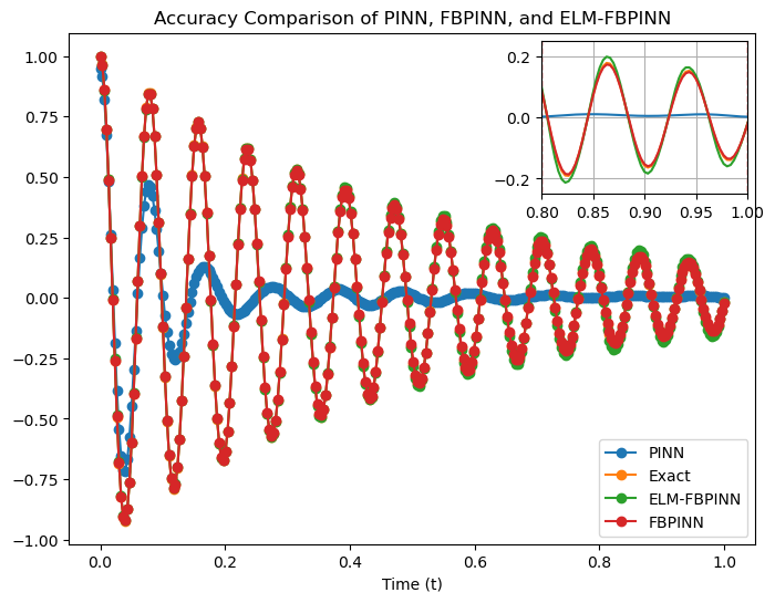
Model	Final $L_{1}$ Loss
PINN	0.226
FBPINN	0.00311
ELM-FBPINN	0.00587

Figure 1: Left: Accuracy comparison for 1D damped harmonic oscillator. Right: Final $L_{1}$ loss values for each method.

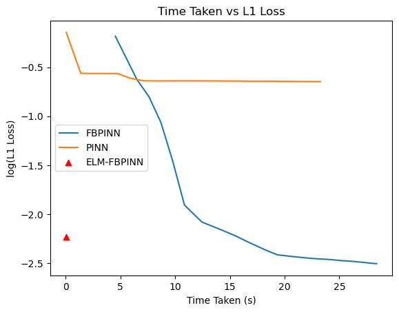
Figure 2: Time (s) vs loss (log) for each method.

Figure 3 shows the relative stability of the size of the (two-norm) condition number of the matrix $(\mathbf{D}_{I}\mathbf{M})^{T}(\mathbf{D}_{I}\mathbf{M})+(\mathbf{D}_{B}\mathbf{B})^{T}(\mathbf{D}_{B}\mathbf{B})$, that arises in the least-squares problem 9, as the number of subdomains changes. The number of subdomains, J, was increased from 5 to 25, with all other parameters kept fixed. While there is some fluctuation in the size of the condition number, the largest network produces a matrix with a similar condition number to the smallest network. This demonstrates that the least-squares problems do not become significantly more challenging to solve as the size of the network increases. Additionally, while the condition number is generally larger than a PINN model of the same size, they are of a similar magnitude, and, crucially, only the ELM-FBPINN results in an accurate approximation of the solution.

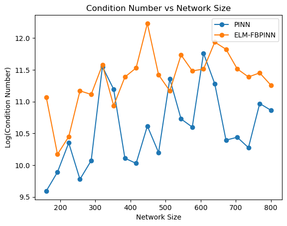
Figure 3: The condition number (log) vs network size for PINN and FBPINN.

5 Discussion and conclusions

For the one-dimensional problem studied, we have shown that the ELM-FBPINN method proposed strongly outperforms a PINN in terms of accuracy and speed. Further, ELM-FBPINN has comparable accuracy to the FBPINN method, while significantly reducing the time taken to optimise parameters. At least for the problems tested, the condition number of the matrix appearing in the ELM-FBPINN least-squares problem 9 appears to be bounded as the number of subdomains increases, indicating that larger problems do not become significantly more challenging to solve. Future work includes investigating the initialisation of untrained weights and biases in the ELM, and the extension to more challenging problems in higher dimensions.

References

- (1) Chen, J., Chi, X., E, W., Yang, Z.: Bridging traditional and machine learning-based algorithms for solving pdes: the random feature method. Journal of Machine Learning 1, 268–98 (2022)
- (2) Dolean, V., Heinlein, A., Mishra, S., Moseley, B.: Finite basis physics-informed neural networks as a Schwarz domain decomposition method. In: Z. Dostál, T. Kozubek, A. Klawonn, U. Langer, L.F. Pavarino, J. Šístek, O.B. Widlund (eds.) Domain Decomposition Methods in Science and Engineering XXVII, pp. 165–172. Springer Nature Switzerland, Cham (2024)
- (3) Dolean, V., Heinlein, A., Mishra, S., Moseley, B.: Multilevel domain decomposition-based architectures for physics-informed neural networks. Computer Methods in Applied Mechanics and Engineering 429, 117116 (2024)
- (4) Huang, G.B., Zhu, Q.Y., Siew, C.K.: Extreme learning machine: Theory and applications. Neurocomputing 70(1), 489–501 (2006). Neural Networks
- (5) Lagaris, I.E., Likas, A., Fotiadis, D.I.: Artificial neural networks for solving ordinary and partial differential equations. IEEE Transactions on Neural Networks 9(5), 987–1000 (1998)
- (6) Moseley, B.: Physics-informed machine learning: from concepts to real-world applications. Ph.D. thesis, University of Oxford (2022)
- (7) Moseley, B., Markham, A., Nissen-Meyer, T.: Finite basis physics-informed neural networks (FBPINNs): a scalable domain decomposition approach for solving differential equations. Advances in Computational Mathematics 49(4), 62 (2023)
- (8) Rahaman, N., Baratin, A., Arpit, D., Draxler, F., Lin, M., Hamprecht, F., Bengio, Y., Courville, A.: On the spectral bias of neural networks. In: K. Chaudhuri, R. Salakhutdinov (eds.) Proceedings of the 36th International Conference on Machine Learning, Proceedings of Machine Learning Research, vol. 97, pp. 5301–5310. PMLR (2019)
- (9) Raissi, M., Perdikaris, P., Karniadakis, G.E.: Physics-informed neural networks: A deep learning framework for solving forward and inverse problems involving nonlinear partial differential equations. Journal of Computational physics 378, 686–707 (2019)
- (10) Wang, S., Wang, H., Perdikaris, P.: On the eigenvector bias of Fourier feature networks: From regression to solving multi-scale PDEs with physics-informed neural networks. Computer Methods in Applied Mechanics and Engineering 384, 113938 (2021)