Spatially-dependent Indian Buffet Processes

Abstract

We develop a new stochastic process called spatially-dependent Indian buffet processes (SIBP) for binary feature matrices of unbounded columns with spatial correlations between subjects, and propose general spatial factor models for various multivariate response variables. We introduce spatial dependency through the stick-breaking representation of the original Indian buffet process (IBP) (Griffiths and Ghahramani, 2005, 2011) and latent Gaussian process for the logit-transformed breaking proportion to capture underlying spatial correlation. We show that the marginal limiting properties of the number of non-zero entries under SIBP are the same as those in the original IBP, while the joint probability is affected by the spatial correlation. Using binomial expansion and Pólya-gamma data augmentation, we provide a novel Gibbs sampler for posterior computation. The usefulness of our SIBP is demonstrated through simulation studies and two applications for large-dimensional multinomial data of areal dialects and geographical distribution of multiple tree species.

Key words: multivariate distribution; nonparametric Bayes; geographical factor; stick-breaking representation

Introduction

The Indian buffet process (IBP) (Griffiths and Ghahramani, 2005) is a powerful model for representing infinite binary matrices, particularly useful for factor models of high-dimensional data. One of the key advantages of the IBP is its ability to automatically determine the number of factors, making it a convenient tool for dimensionality reduction and feature extraction. Additionally, factor analysis using the IBP can also produce clustering results. Unlike traditional methods like $K$-means clustering, the binary representations proposed by IBP allow for capturing similarities between clusters and representing numerous clusters with only a small number of factors. See Griffiths and Ghahramani (2011) for an introduction and review of IBP.

A potential limitation of the standard IBP is that it does not incorporate spatial information. This omission may lead to overlooking spatial heterogeneity and correlations, potentially resulting in inadequate factor representations. For example, when analyzing dialect data collected from various regions (a high-dimensional categorical dataset) as used in Section 5.1, it is natural to assume that geographically close areas would share similar linguistic structures. However, standard IBP models cannot capture such spatial information. Therefore, there is a need to develop a generalized version of IBP that can account for geographical relationships and spatial dependencies for successfully applying the IBP to multivariate spatial data.

To address the aforementioned issue, we introduce spatially-dependent Indian buffet processes (SIBP) using a stick-breaking representation, which can effectively incorporate geographical information into the modeling of multivariate binary factors. This approach enhances the flexibility and accuracy of the model in capturing spatial dependencies and automatically determines the optimal number of latent factors needed for a given dataset. To complement this modeling framework, we develop a highly efficient Markov Chain Monte Carlo (MCMC) computation algorithm. This algorithm leverages a novel data augmentation strategy that combines the binomial expansion and well-known Pólya-gamma distribution (Polson et al., 2013), which enables to carry out the posterior computation by a Gibbs sampler.

There have been several attempts to extend the standard IBP models. The dependent Indian buffet process (Williamson et al., 2010) introduces a stochastic process for a binary matrix $Z(t)$ indexed by $t$, which differs from our proposal as our method introduces spatial correlation within the elements of a binary matrix $Z$. Stolf and Dunson (2024) proposed the multivariate probit Indian buffet process that accounts for correlations among different features but assumes independence among subjects, unlike our proposal. Warr et al. (2022) and Gershman et al. (2014) introduce the distance-based Indian buffet process, incorporating distance information using the Chinese restaurant representation for the IBP. However, it defines a multivariate model only for the observed locations, and construction is not process-based, making the prediction of unobserved locations unjustifiable. There have been other various works on generalizations of the classical IBP model (e.g. Broderick et al., 2013; Di Benedetto et al., 2020; Camerlenghi et al., 2024), but to the best of our knowledge, this work is the first one to propose a process-based model that generalizes the standard IBP to incorporate spatial information. The formulation of SIBP is also related to the stick-breaking representation of the Dirichlet process, and there are several works on introducing latent distributions for the transformed proportions (e.g. Rodríguez et al., 2010; Ren et al., 2011; Grazian, 2024). However, the posterior distribution of the SIBP model is considerably different from those under the Dirichlet process model, so the existing sampling techniques for the Dirichlet process cannot be directly incorporated into the SIBP model.

This paper is organized as follows. Section 2 introduces the proposed SIBP and discusses its theoretical properties. In Section 3.2, an efficient posterior computation algorithm for general latent variable models with SIBP is discussed. The numerical performance is demonstrated using simulation experiments in Section 4 and applications to two types of datasets in Section 5. Technical proofs are provided in the appendix.

Spatially-dependent Indian Buffet Process

Indian buffet process and stick-breaking representations

Let $Z$ be a binary feature matrix, with $n$ rows for subjects and an unbounded number of columns for features, where each element $z_{ik}\in\{0,1\}$ indicates whether the $i$th subject possess the $k$th feature (i.e., $z_{ik}=1$) or not. In the Indian buffet metaphor, the rows of $Z$ represent customers, and the columns represent dishes, with $Z$ being constructed through a sequential sampling process. The first customer enters the restaurant and selects dishes according to ${\rm Po}(\alpha)$ with a parameter $\alpha$. For the $i$th customer, they sample each dish that has been previously taken with a probability of $m_{k}/i$, where $m_{k}$ denotes the number of prior customers who have chosen dish $k$. Additionally, the $i$th customer selects new dishes based on ${\rm Po}(\alpha/i)$. The selection of dishes by each customer can be represented in a binary feature allocation matrix $Z$. Such process is called Indian Buffet Process (IBP) (Griffiths and Ghahramani (2005, 2011)) and is denoted by ${\rm IBP}(\alpha)$.

As shown in Griffiths and Ghahramani (2011), the IBP can also be defined as the limit of a Beta-Bernoulli model. Here we consider the following latent variable model with finite $K$ features:

$$z_{ik}\sim{\rm Bernoulli}\,(b_{k}),\quad b_{k}\sim{\rm Beta}\left(\frac{\alpha}{K},1\right),$$ (1)

with a parameter $\alpha$, where the $b_{k}$ are generated independently and each $z_{ik}$ is independent of all other assignments under given $b_{k}$. Griffiths and Ghahramani (2011) showed that the distribution of $Z$ under $K\to\infty$ is equivalent to the one obtained by IBP. The IBP has several desirable properties. In particular, the expectation of the number of features possessed by each object under $K\to\infty$ is $\alpha$, which indicates the sparsity of feature selection. As an alternative representation of the Beta-Bernoulli model of (1), Teh et al. (2007) introduced the stick-breaking representation of (1) under finite $K$, given by

$$z_{ik}\sim{\rm Bernoulli}\,(b_{k}),\quad b_{k}=\prod_{j=1}^{k}\,v_{j},\ \ \ k=1,\ldots,K,$$

where $v_{j}\sim{\rm Beta}(\alpha,1)$. The above representation guarantees that the sequence $b_{1},\ldots,b_{K}$ is strictly decreasing. We leverage this representation to introduce spatial correlation in the subsequent section.

Spatially-dependent IBP

To take account of spatial information, let $z_{k}(s)$ is a binary random variable at location $s$ and consider the following model:

$$z_{k}(s)\sim{\rm Bernoulli}\,(b_{k}(s)),\quad b_{k}(s)=\prod_{j=1}^{k}\,\sigma(u_{j}(s)),\ \ \ k=1,\ldots,K,$$ (2)

where $\sigma(x)=1/(1\!+\!e^{-x})$ is a logistic function and $u_{j}(s)$ follows a Gaussian process, independently for $j=1,\ldots,K$. We call Spatially-dependent Indian buffet process (SIBP) of the process (2). The process (2) can be regarded as an extension of the logistic stick-breaking process (Ren et al., 2011). For $n$ locations denoted by $s_{1},\ldots,s_{n}$, the joint model for $z_{ik}\equiv z_{k}(s_{i})\ (i=1,\ldots,n)$ is described as

$$z_{ik}\sim{\rm Bernoulli}\,(b_{ik}),\quad b_{ik}=\prod_{j=1}^{k}\,\sigma(u_{ij}),\ \ \ k=1,\ldots,K.$$ (3)

Here $u_{ik}$ is a continuous latent variable and the joint distribution is

$$u_{k}\equiv(u_{1k},\ldots,u_{nk})\sim N_{n}(\mu 1_{n},\tau^{-1}Q(\psi))$$

independently for $k=1,\ldots,K$, where $\mu$ is a location parameter, $1_{n}$ is an $n$-dimensional vector of $1$, $\tau$ is a precision parameter and $Q(\psi)$ is a correlation matrix parametrized by $\psi$. One example of $Q(\psi)$ is that its $(i,i^{\prime})$-element is $\rho(d_{ii^{\prime}};\psi)$, where $d_{ii^{\prime}}$ denotes some distance between $i$th and $i^{\prime}$th locations. Standard choices are the Matérn function, $\rho(d;\psi)=\{2^{\kappa-1}\Gamma(\kappa)\}^{-1}(d/\phi)^{\kappa}K_{\kappa}(d/\phi)$ with $\psi=(\phi,\kappa)$ and the exponential function, $\rho(d;\psi)=\exp(-d/\phi)$, where $\phi>0$ is a spatial range parameter and $\kappa>0$ is a smoothness parameter. Here $K_{\kappa}(\cdot)$ denotes the modified Bessel function of the third kind of order $\kappa$. We call Spatially-dependent Indian buffet process (SIBP) of the model (3) with spatially correlated latent variable $u_{ik}$. It should be noted that when the spatial range parameter is very large, the covariance matrix $Q(\psi)$ is degenerate and it holds that $u_{1k},\ldots,u_{nk}$ are identical with probability one and follow $N(\mu,\tau^{-1})$. This corresponds to the stick-breaking representation of IBP with different distributional assumptions for $v_{k}$.

Properties of SIBP

We present some theoretical properties of SIBP. First, we prove that the expected number of non-zero entries is finite in the limiting case.

Proposition 1.

The binary matrix generated by SIBP is sparse, that is, $P(z_{ik}=1)\to 0$ as $k\to\infty$. Further, let $c_{i}=\sum_{j=1}^{k}z_{ij}$ be the number of features that the $i$th subject possess. Then, $\lim_{k\to\infty}E[c_{i}]=\delta_{1}/(1-\delta_{1})$ and

$$\lim_{k\to\infty}{\rm Var}(c_{i})=\frac{\delta_{1}}{1-\delta_{1}}\left(1+\frac{2\delta_{2}}{1-\delta_{2}}-\frac{\delta_{1}}{1-\delta_{1}}\right)$$

for each $i=1,\ldots,n$, where

$$\delta_{p}=\int_{-\infty}^{\infty}\sigma(x)^{p}\phi(x;\mu,\tau^{-1})dx,\ \ \ \ p=1,2$$

are constants dependent on $\mu$ and $\tau$.

The Proposition 1 ensures that the number of sampled features is finite, namely, $P(c_{i}<\infty)=1$. Furthermore, it can be seen that the expectation of the total number of non-zero elements is $n\delta_{1}/(1-\delta_{1})$. Further, when $\mu$ and $\tau$ are chosen such that $2\delta_{2}/(1-\delta_{2})=\delta_{1}/(1-\delta_{1})$, the limit of $E[c_{i}]$ and ${\rm Var}(c_{i})$ are the same as the standard IBP. It should also be noted that the spatial range parameter $\psi$ (controlling the correlation given a fixed distance) in the Gaussian process does not appear in the formula. This indicates that the basic performance of SIBP depends only on the parameters, $\mu$ and $\tau$, of the marginal distributions.

We next investigate how the spatial correlation is introduced in the generated binary matrices through the latent Gaussian process. To this end, we evaluate the joint probability that two binary variables are both 1, as given in the following proposition:

Proposition 2.

Under the SIBP model, $P(z_{ik}=1,z_{jk}=1)=D_{\mu,\tau}(\rho_{ij})^{k}$ for each $i,j=1,\ldots,n$, where $D_{\mu,\tau}(\rho_{ij})=E[\sigma(u_{ik})\sigma(u_{jk})]$ and the expectation is taken with respect to $(u_{ik},u_{jk})\sim N_{2}((\mu,\mu),\Sigma)$ with $\Sigma_{11}=\Sigma_{22}=1/\tau$, $\Sigma_{12}=\Sigma_{21}=\rho_{ij}/\tau$ and $\rho_{ij}=\rho(\|s_{i}-s_{j}\|;\psi)$. Furthermore, $D_{\mu,\tau}(\rho)$ is an increasing function of $\rho\in(0,1)$.

Proposition 2 indicates that the probability that the two subjects possess the $j$th feature simultaneously is dictated by the spatial correlation $\rho_{ij}$ and the spatial range parameter $\psi$.

We next consider the number of (non-null) common features, defined as $K^{\ast}=\sum_{k=1}^{K}I(c_{k}>0)$, where $c_{k}=\sum_{i=1}^{n}z_{ik}$. Then, it holds that

$$E[K^{\ast}]=\sum_{k=1}^{K}P(c_{k}>0) =\sum_{k=1}^{K}\bigg{\{}1-P(z_{1k}=0,\ldots,z_{nk}=0)\bigg{\}}$$

$$=\sum_{k=1}^{K}\bigg{\{}1-E\bigg{[}\prod_{i=1}^{n}\Big{(}1-\prod_{j=1}^{k}\sigma(u_{ij})\Big{)}\bigg{]}\bigg{\}},$$

where the expectation is taken with respect to the joint distribution of $u_{k}\sim N(\mu 1_{n},\tau^{-1}Q(\psi))$. Although the above expectation cannot be expressed in a closed form, we simulated the expectations by Monte Carlo integration under various choices of $(\mu,\tau,\psi)$. Specifically, we consider the exponential covariance function, $Q(\psi)_{ij}=\exp(\|s_{i}-s_{j}\|/\psi)$, and generated the location information from the uniform distribution on $[0,1]\times[0,1]$. Regarding the parameter values, we consider all the combinations of $\mu\in\{-1,0,1\}$, $\tau\in\{0.5,1\}$ and $\psi\in\{0.2,0.5,1\}$. In Figure 1, we show $E[K^{\ast}]$ as a function of the sample size. The results indicate that the parameter $\mu$ significantly controls the number of features, that is, larger value of $\mu$ leads to larger number of features in the prior distribution. On the other hand, $\tau$ and $\psi$ do not affect much on the number of features.

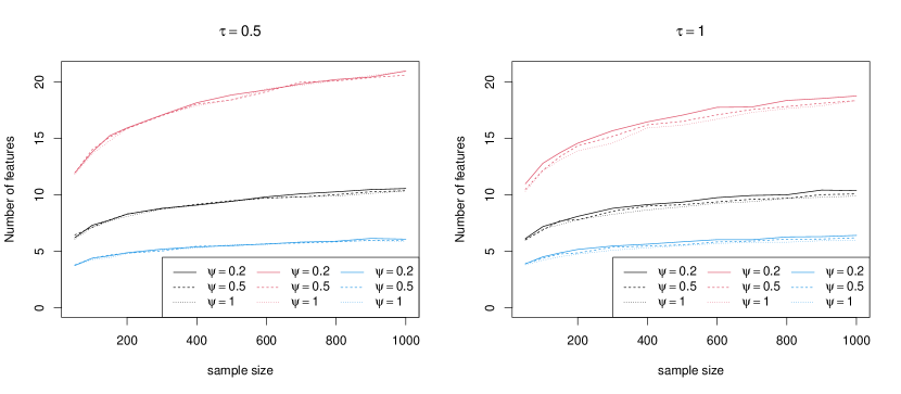
Figure 1: Number of common factors under SIBP with $\mu=-1$ (blue), $\mu=0$ (black), and $\mu=1$ (red), as a function of sample size.

Implementation of SIBP

Latent variable models with SIBP

Let $x_{1},\ldots,x_{n}$ be an observed data, and $s_{i}\ (i=1,\ldots,n)$ be a location information (e.g., longitude and latitude) associated with $x_{i}$. We consider the following latent variable model:

$$\begin{split}&x_{i}\sim f\left(x_{i}\mid\{z_{ik}\}_{k=1}^{K};\{\theta_{k}\}_{k=1}^{K}\right),\quad z_{ik}\sim{\rm Bernoulli}\Big{(}\prod_{j=1}^{k}\sigma(u_{ij})\Big{)},\ \ \ i=1,\ldots,n,\\ &(u_{1k},\ldots,u_{nk})\sim N_{n}(\mu 1_{n},\tau^{-1}Q(\psi)),\ \ \ \ k=1,\ldots,K,\end{split}$$ (4)

where $f(x_{i}\mid\{z_{ik}\}_{k=1}^{K};\{\theta_{k}\}_{k=1}^{K})$ is a density (or probability) function of $x_{i}$. Note that $\theta_{k}$ is related to the distribution of $x_{i}$, and $(u_{1k},\ldots,u_{nk})$ are independent for $k=1,\ldots,K$. The unknown parameters in the latent variable model (4) are $\theta_{k}$, $\tau$, and $\psi$, for which we assign prior distributions for Bayesian inference. In particular, we employ a conditionally conjugate prior, $\tau\sim{\rm Ga}(a_{\tau},b_{\tau})$, $\mu\sim{\rm N}(m_{\mu},S_{\mu})$ and gamma priors for each element of $\psi$. Regarding the prior for $\theta_{k}$, we use a class of repulsive prior (e.g. Petralia et al., 2012; Xie and Xu, 2020) instead of assuming independent priors for $\theta_{1},\ldots,\theta_{K}$ to prevent redundant expression of the latent factors. Let $\pi(\theta_{k})$ be a marginal prior of $\theta_{k}$. Then, the repulsive prior for $\theta_{1},\ldots,\theta_{K}$ is given by

$$\pi(\theta_{1},\ldots,\theta_{K})=\frac{1}{Z_{K}}\left\{\prod_{k=1}^{K}\pi(\theta_{k})\right\}\min_{1\leq k<k^{\prime}\leq K}g(\|\theta_{k}-\theta_{k^{\prime}}\|),$$

where $Z_{K}$ is a normalizing constant and $g:\mathcal{R}_{+}\to[0,1]$ is a strictly increasing function with $g(0)=0$. The repulsive prior eliminates the prior mass from the region where $\theta_{k}$ and $\theta_{k^{\prime}}$ are close. For the specific choice of $g(\cdot)$, we use $g(x)=I(x>\delta)(1-\delta/x)$ with a tuning constant $\delta>0$. Since the results would not be sensitive to the choice of $\delta$ as long as $\delta$ is small, we set $\delta=10^{-3}$ throughout the numerical studies in this paper.

Posterior computation via Gibbs sampler

For a general latent variable model with SIBP (4), we here provide a Gibbs sampler to simulate the posterior distributions by using a novel combination of binomial expansion and the Pólya-gamma data augmentation (Polson et al., 2013). Define $Z$, $U$ and $\Theta$ be sets of $z_{ik}$, $u_{ik}$ and $\theta_{k}$, respectively. Under the prior for these parameters, the joint posterior distribution $\pi(Z,U,\Theta,\tau,\psi|D)$ of the latent variables ($Z$ and $U$) and unknown parameters ($\Theta,\tau$ and $\psi$) given a set of observed data $D=\{x_{1},\ldots,x_{n}\}$ can be expressed as

$$\pi(Z,U,\Theta,\tau,\psi\mid D) \propto\prod_{i=1}^{n}\prod_{k=1}^{K}f(x_{i}\mid\{z_{ik}\}_{k=1}^{K};\{\theta_{k}\}_{k=1}^{K})\Big{\{}\prod_{j=1}^{k}\sigma(u_{lj})\Big{\}}^{z_{ik}}\Big{\{}1-\prod_{j=1}^{k}\sigma(u_{lj})\Big{\}}^{1-z_{ik}}$$

$$\ \ \ \ \times p(\tau)p(\psi)\pi(\theta_{1},\ldots,\theta_{K})\prod_{k=1}^{K}\phi(u_{k};\mu 1_{n},\tau^{-1}Q(\psi)).$$

We use Gibbs sampling to generate random samples from the above posterior distribution. The details are described as follows:

• (Update of $u_{k}$)  For each $i$ and $k$, the full conditional distribution of $u_{k}$ is proportional to

  $$\phi(u_{k};\mu 1_{n},\tau^{-1}Q(\psi))\prod_{i=1}^{n}\prod_{j=k}^{K}\sigma(u_{ik})^{z_{ij}}\bigg{\{}1-\sigma(u_{ik})\prod_{h=1,h\neq k}^{j}\sigma(u_{ih})\bigg{\}}^{1-z_{ij}}$$

  $$= \ \phi(u_{k};\mu 1_{n},\tau^{-1}Q(\psi))\prod_{i=1}^{n}\prod_{j=k}^{K}\frac{(e^{u_{ik}})^{z_{ij}}(1+C_{ikj}e^{u_{ik}})^{1-z_{ij}}}{1+e^{u_{ik}}},$$

  where $C_{ikj}=1-\prod_{h=1,h\neq k}^{j}\sigma(u_{ih})\in(0,1)$. By introducing latent binary variables, $s_{ikj}$ for $j=k,\ldots,K$ with $P(s_{ikj}=1)=C_{ikj}/(1+C_{ikj})$, the likelihood term can be augmented as

  $$\prod_{j=k}^{K}\frac{(e^{u_{iik}})^{z_{ij}}(e^{u_{ik}})^{(1-z_{ij})s_{ikj}}}{1+e^{u_{ik}}}=\frac{(e^{u_{ik}})^{\sum_{j=k}^{K}\{z_{ij}+(1-z_{ij})s_{ikj}\}}}{(1+e^{u_{ik}})^{K-k+1}}.$$

  Note that the full conditional probability being $s_{ikj}=1$ is $C_{ikj}e^{u_{ik}}/(C_{ikj}e^{u_{ik}}+e^{u_{ik}z_{ij}})$. Then, applying the Pólya-gamma data augmentation (Polson et al., 2013), the above function can be expressed as

  $$\frac{(e^{u_{ik}})^{\sum_{j=k}^{K}\{z_{ij}+(1-z_{ij})s_{ikj}\}}}{(1+e^{u_{ik}})^{K-k+1}}\propto\exp(\kappa_{ik}u_{ik})\int_{0}^{\infty}\exp\left(-\frac{1}{2}\omega_{ik}u_{ik}^{2}\right)f_{\rm PG}(\omega_{ik}|K-k+1,0)d\omega_{ik},$$

  where $f_{\rm PG}(\cdot|b,c)$ is the density function of ${\rm PG}(b,c)$ and

  $$\kappa_{ik}=\sum_{j=k}^{K}\{z_{ij}+(1-z_{ij})s_{ikj}\}-\frac{1}{2}(K-k+1).$$

  Note that the full conditional distribution of $\omega_{ik}$ is ${\rm PG}(K-k+1,u_{ik})$. Using the augmentation, the full conditional distribution of $u_{k}$ is $N(A_{k}^{-1}B_{k},A_{k}^{-1})$, where

  $$A_{k}={\rm diag}(\omega_{1k},\ldots,\omega_{nk})+\tau Q(\psi)^{-1},\ \ \ B_{k}=(\kappa_{1k},\ldots,\kappa_{nk})^{\top}+\tau Q(\psi)^{-1}1_{n}\mu.$$

• (Update of $z_{i1},\ldots,z_{iK}$)  For each $i$, the full conditional distribution of $(z_{i1},\ldots,z_{iK})$ is proportional to

  $$f\big{(}x_{i}\mid\{z_{ik}\}_{k=1}^{K};\{\theta_{k}\}_{k=1}^{K}\big{)}\bigg{\{}\prod_{k=1}^{K}\sigma(u_{ik})\bigg{\}}^{z_{ik}}\bigg{\{}1-\prod_{k=1}^{K}\sigma(u_{ik})\bigg{\}}^{1-z_{ik}}.$$

  When $K$ is not large (e.g., $K<8$), we can compute the above (unnormalized) probability on $(z_{i1},\ldots,z_{iK})\in\{0,1\}^{K}$, and update the binary vector $(z_{i1},\ldots,z_{iK})$ simultaneously. When $K$ is large, one can update $z_{ik}$ separately by computing the full conditional probability of $z_{ik}=1$.

• (Update of $\theta_{k}$)  For each $k$, the full conditional of $\theta_{k}$ is proportional to

  $$\pi(\theta_{k})\prod_{i=1}^{n}f\big{(}x_{i}\mid\{z_{ij}\}_{j=1}^{K};\{\theta_{j}\}_{j=1}^{K}\big{)}\min_{1\leq k^{\prime}\leq K,k^{\prime}\neq k}g(\|\theta_{k}-\theta_{k^{\prime}}\|),$$

  and the specific sampling algorithms depend on the distributional assumption for $x_{i}$. A typical strategy is to generate a proposal $\theta_{k}^{\ast}$ from a distribution proportional to $\pi(\theta_{k})\prod_{i=1}^{n}f\big{(}x_{i}\mid\{z_{ij}\}_{j=1}^{K};\{\theta_{j}\}_{j=1}^{K}\big{)}$ and accept it with probability

  $$\min_{1\leq k^{\prime}\leq K,k^{\prime}\neq k}g(\|\theta_{k}^{\ast}-\theta_{k^{\prime}}\|)/\min_{1\leq k^{\prime}\leq K,k^{\prime}\neq k}g(\|\theta_{k}^{\dagger}-\theta_{k^{\prime}}\|),$$

  for the current value $\theta_{k}^{\dagger}$

• (Update of $\tau$)  The full conditional of $\tau$ is ${\rm Ga}(\tilde{a}_{\tau},\tilde{b}_{\tau})$, where $\tilde{a}_{\tau}=a_{\tau}+nK/2$ and $\tilde{b}_{\tau}=b_{\tau}+\frac{1}{2}\sum_{k=1}^{K}(u_{k}-\mu 1_{n})^{\top}Q(\psi)^{-1}(u_{k}-\mu 1_{n})/2$.

• (Update of $\mu$)  The full conditional of $\mu$ is $N(A_{\mu}^{-1}B_{\mu},A_{\mu}^{-1})$, where $A_{\mu}=K\tau 1_{n}^{\top}Q(\psi)^{-1}1_{n}+S_{\mu}^{-1}$ and $B_{\mu}=\tau 1_{n}^{\top}Q(\psi)^{-1}\sum_{k=1}^{K}u_{k}+S_{\mu}^{-1}m_{\mu}$.

• (Update of $\psi$)  The full conditional of $\psi$ is proportional to

  $$\pi(\psi)|Q(\psi)|^{-K/2}\exp\left\{-\frac{\tau}{2}\sum_{k=1}^{K}(u_{k}-\mu 1_{n})^{\top}Q(\psi)^{-1}(u_{k}-\mu 1_{n})\right\},$$

  for which we use a random-walk Metropolis-Hastings algorithm.

The above Gibbs sampling algorithm can be easily implemented since most of the full conditional distributions are familiar due to the binomial expansion and Pólya-gamma data augmentation.

Owing to the Gaussian process assumption, we can predict latent binary vectors in (arbitrary) unobserved locations. Let $s$ be an unobserved location of interest. Then, the conditional distribution of $u_{k}(s)$ given $u_{k}=(u_{1k},\ldots,u_{nk})$ is $N(\mu+C(s)(u_{k}-\mu 1_{n}),\tau^{-1}-\tau^{-1}C(s)Q(\psi)^{-1}C(s))$, where $C(s)=(\rho(d(s,s_{1});\psi),\ldots,\rho(d(s,s_{n});\psi))$ and $d(s,s_{1})$ is a distance between unobserved location $s$ and observed location $s_{i}$. Hence, one can easily simulate the binary indicator $z_{k}(s)$ at site $s$ based on the posterior predictive distribution of $v_{k}(s)\equiv\prod_{j=1}^{k}u_{k}(s)$.

Scalable implementation of SIBP

When the number of locations, $n$, is large, the posterior computational cost may be intensive due to the Gaussian process assumption for the latent variable $u_{ik}$. To make the proposed method scalable under a large number of locations, we adopt the nearest-neighbor Gaussian process (Datta et al., 2016). Instead of the Gaussian process model in (1), we employ the following model:

$$\pi(u_{1k},\ldots,u_{nk})=\prod_{i=1}^{n}\phi(u_{ij};B_{i}u_{j}(N(s_{i})),\tau^{-1}F_{i}),\ \ \ \ j=0,\ldots,J$$ (5)

where $N_{i}$ is the set of $m$-nearest neighbors of the location $s_{i}$, $u_{j}(N(s_{i}))$ is a sub-vector of $u_{j}$ collecting random variables on the $m$-nearest neighbors of $s_{i}$, and

$$B_{i}=Q_{s_{i},N(s_{i})}(\psi)Q_{N(s_{i})}(\psi)^{-1},\ \ \ \ F_{i}=\tau^{-1}-\tau^{-1}Q_{s_{i},N(s_{i})}(\psi)Q_{N(s_{i})}(\psi)^{-1}Q_{N(s_{i}),s_{i}}(\psi).$$

Here $Q_{s_{i},N(s_{i})}(\psi)\equiv{\rm Cor}(u_{ji},u_{j}(N(s_{i})))$ and $Q_{N(s_{i})}(\psi)\equiv{\rm Cor}(u_{j}(N(s_{i})),u_{j}(N(s_{i})))$ are respectively sub-vector and sub-matrix of $Q(\psi)$. Under the model, the full conditional distribution of $u_{ij}$ is also normal as in the standard Gaussian process, so we can use a similar Gibbs sampling algorithm under the nearest-neighbor Gaussian process.

Example 1: Spatial factor models for large-dimensional multinomial data

To reveal the differences in the geographical distribution of dialects for various meanings, as considered in Section 5.1, we need to deal with large-dimensional multinomial data. Let $x_{i}=(x_{i1},\ldots,x_{iM})$ be an $M$-dimensional vector of multinomial observations, where $x_{im}$ takes one of $\{1,\ldots,c_{m}\}$ for $m=1,\ldots,M$ and $i=1,\ldots,n$. Here $n$ is the number of areas and $M$ is the number of meanings, which could be large to achieve appropriate characterization of each dialect. Further, let $\pi_{iml}\ (l=1,\ldots,c_{m})$ be a multinomial probability, so that $x_{im}$ is generated from the categorical distribution on $\{1,\ldots,c_{m}\}$ with probability $(\pi_{im1},\ldots,\pi_{imc_{m}})$.

In this setting, we are interested in low-dimensional representations of the difference of dialects. To this end, we model the probability as

$$\pi_{iml}=\frac{\exp\big{(}\eta_{ml}+\sum_{k=1}^{K}z_{ik}\theta_{kml}\big{)}}{\sum_{l^{\prime}=1}^{c_{m}}\exp\big{(}\eta_{ml^{\prime}}+\sum_{k=1}^{K}z_{ik}\theta_{kml^{\prime}}\big{)}},\ \ \ \ l=1,\ldots,c_{m},$$

where $(\eta_{m1},\ldots,\eta_{mc_{m}})$ is a baseline common to all the areas and $\theta_{kml}$ is a continuous value of $k$th factor. Note that we set $\eta_{m1}=0$ and $\theta_{km1}=0$ for identifiability. We further assume that $\eta_{ml}\sim N(0,\gamma_{0}^{-1})$ and $\theta_{kml}\sim N(0,\gamma_{k}^{-1})$ independently for $m=1,\ldots,M$ and $l=2,\ldots,c_{m}$. Note that the distribution of $x_{i}$ is

$$f\big{(}x_{i}\mid\{z_{ik}\}_{k=1}^{K};\{\theta_{k}\}_{k=1}^{K},\eta\big{)}=\prod_{m=1}^{M}\prod_{l=1}^{c_{m}}\left[\frac{\exp\big{(}\eta_{ml}+\sum_{k=1}^{K}z_{ik}\theta_{kml}\big{)}}{\sum_{l^{\prime}=1}^{c_{m}}\exp\big{(}\eta_{ml^{\prime}}+\sum_{k=1}^{K}z_{ik}\theta_{kml^{\prime}}\big{)}}\right]^{I(x_{im}=l)},$$

so that we can generate $z_{i}$, $u_{k}$, $\tau_{k}$ and $\psi_{k}$ through their full conditional distributions as given in Section 3.2. On the other hand, the full conditional of $\Theta_{ml}=(\eta_{ml},\theta_{1ml},\ldots,\theta_{Kml})$ is

$$\phi_{K+1}(\Theta_{ml};0,\Gamma^{-1})\prod_{i=1}^{n}\frac{\exp\big{(}\eta_{ml}+\sum_{k=1}^{K}z_{ik}\theta_{kml}\big{)}^{I(x_{im}=l)}}{\sum_{l^{\prime}=1}^{c_{m}}\exp\big{(}\eta_{ml^{\prime}}+\sum_{k=1}^{K}z_{ik}\theta_{kml^{\prime}}\big{)}}$$

$$\propto\ \phi_{K+1}(\Theta_{ml};0,\Gamma^{-1})\prod_{i=1}^{n}\frac{\exp\big{(}z_{i}^{\top}\Theta_{ml}-C_{iml}\big{)}^{I(x_{im}=l)}}{1+\exp\big{(}z_{i}^{\top}\Theta_{ml}-C_{iml}\big{)}},$$

where $\Gamma={\rm diag}(\gamma_{0},\gamma_{1},\ldots,\gamma_{K})$, $z_{i}=(1,z_{i1},\ldots,z_{iK})$ and $C_{iml}=\sum_{l^{\prime}=1,l^{\prime}\neq l}^{c_{m}}\exp\big{(}z_{i}^{\top}\Theta_{ml^{\prime}})$. Using the Pólya-gamma data augmentation (Polson et al., 2013), the above distribution can be augmented as

$$\phi_{K+1}(\Theta_{ml};0,\Gamma^{-1})\prod_{i=1}^{n}\exp\Big{\{}\kappa_{iml}(z_{i}^{\top}\Theta_{ml}-C_{iml})-\frac{1}{2}\omega_{ml}(z_{i}^{\top}\Theta_{ml}-C_{iml})^{2}\Big{\}}f_{\rm PG}(\omega_{iml};1,0),$$

where $\kappa_{iml}=I(x_{im}=l)-1/2$. The full conditional of $\omega_{iml}$ is ${\rm PG}(1,z_{i}^{\top}\Theta_{ml}-C_{iml})$, and that of $\Theta_{ml}$ is $N(A_{ml}^{-1}B_{ml},A_{ml}^{-1})$, where

$$A_{ml}=\sum_{i=1}^{n}\omega_{iml}z_{i}z_{i}^{\top}+\Gamma^{-1},\ \ \ \ B_{ml}=\sum_{i=1}^{n}z_{i}(\kappa_{iml}+\omega_{iml}C_{iml}).$$

Example 2: Spatial factor models for multivariate count data

To investigate the vegetation of multiple species of trees in Japan, considered in Section 5.2, we want to extract spatial factors regarding the geographical distributions of multiple species of trees. To this end, we consider the case with multivariate count response. Let $x_{i}=(x_{i1},\ldots,x_{iM})$ be an $M$-dimensional vector of count observations. For each element $x_{im}$, we assume that

$$x_{im}\sim{\rm NB}(\lambda_{im},\nu_{m}),\ \ \ \lambda_{im}=\exp\left(\eta_{m}+\sum_{k=1}^{K}z_{ik}\theta_{km}\right),$$

where $\nu_{m}$ is a dispersion parameter, $\eta_{m}$ is a baseline term and $(\theta_{k1},\ldots,\theta_{kM})$ is a vector of mean parameters for the $k$th factor. Note that the distribution of $x_{i}$ is

$$f(x_{i}\mid\{z_{ik}\}_{k=1}^{K};\{\theta_{k}\}_{k=1}^{K},\eta)=\prod_{m=1}^{M}\frac{\Gamma(\nu_{m}+x_{im})}{\Gamma(\nu_{m})x_{im}!}\left(\frac{\nu_{m}}{\nu_{m}+\lambda_{im}}\right)^{\nu_{m}}\left(\frac{\lambda_{im}}{\nu_{m}+\lambda_{im}}\right)^{x_{im}}$$

so that $E[x_{im}]=\lambda_{im}$ and ${\rm Var}(x_{im})=\lambda_{im}+\lambda_{im}^{2}/\nu_{m}$.

We assign prior distributions, $\nu\sim{\rm Ga}(a_{\nu},b_{\nu})$, $\eta_{m}\sim N(0,\gamma_{0}^{-1})$ and $\theta_{km}\sim N(0,\gamma_{k}^{-1})$ independently for $m=1,\ldots,M$. Note that the sampling algorithm for parameters other than $\nu_{m},\eta_{m}$ and $\theta_{km}$ is the same as in Section 3.2. The detailed sampling algorithm for these parameters is given as follows:

• (Sampling from $\Theta_{m}=(\eta_{m},\theta_{1m},\ldots,\theta_{Km}$)   Using the Pólya-gamma data augmentation, we first generate latent variable $\omega_{im}$ from ${\rm PG}(x_{im}+\nu_{m},\eta_{m}+\sum_{k=1}^{K}z_{ik}\theta_{km}-\log\nu_{m})$. Then one can generate $\Theta_{m}$ from $N(A_{m}^{-1}B_{m},A_{m}^{-1})$, where

  $$A_{m}=\sum_{i=1}^{n}\omega_{im}z_{i}z_{i}^{\top}+\Gamma^{-1},\ \ \ \ B_{m}=\sum_{i=1}^{n}z_{i}(\kappa_{im}+\omega_{im}\log\nu_{m}).$$

  and $\kappa_{im}=(x_{im}-\nu_{m})/2$. Here $\Gamma={\rm diag}(\gamma_{0},\gamma_{1},\ldots,\gamma_{K})$, $z_{i}=(1,z_{i1},\ldots,z_{iK})$.

• (Sampling from $\nu_{m}$)   For $m=1\ldots,M$, we employ a random-walk Metropolis-Hastings algorithm.

Simulation Study

Recovery of latent factors

We first demonstrate the numerical performance of the proposed SIBP through the multinomial models introduced in Section 3.4. For $i=1,\ldots,n$, we let $x_{i}=(x_{i1},\ldots,x_{iM})$ with be a observed vector, where $x_{im}\ (m=1,\ldots,M)$ independently follows a multinomial distribution on $\{1,\ldots,L\}$ with probability $\pi_{iml}\ (l=1,\ldots,L)$. Further, let $s_{i}=(s_{i1},s_{i2})$ be the two-dimensional vector of location information generated from the uniform distribution on $[-1,1]\times[-1,1]$. We set $n=80$, $M=50$ and $L=5$ in this study. We consider the following true structure of the multinomial probability $\pi_{iml}$:

$$\pi_{iml}=\frac{\exp(\sum_{k=1}^{K^{\ast}}z_{ik}\theta_{kml})}{\sum_{l^{\prime}=1}^{L}\exp(\sum_{k=1}^{K^{\ast}}z_{ik}\theta_{kml^{\prime}})},$$

where $z_{ik}$ is a binary variable and $\theta_{kml}$ determines the effects of the $k$th latent factor. We adopt the latent factor defined as

$${\rm(I)}\ \ \ \ z_{i1}=I(s_{i1}^{2}+s_{i2}^{2}<(0.9)^{2}),\ \ \ \ z_{i2}=I(s_{i1}<0.5,s_{i2}>0),\ \ \ \ z_{i3}=I(s_{i1}<s_{i2}-0.7),$$

$$\theta_{1ml}\sim N(1,1),\ \ \ \ \theta_{2ml}\sim N(0.5,(1.5)^{2})),\ \ \ \ \theta_{3ml}\sim N(0,4),$$

where $K^{\ast}=3$ as the true number of latent factors. The realized location information and true clustering structures are shown in the top row of Figure 2. Note that $\sum_{i=1}^{n}z_{i1}=56$, $\sum_{i=1}^{n}z_{i2}=27$ and $\sum_{i=1}^{n}z_{i3}=15$.

Based on the generated data $(x_{i},s_{i})$, we fitted the multinomial factor model described in Section 3.4 with the proposed SIBP and the standard IBP. We set $K=10$, the maximum number of factors in both SIBP and IBP models. We generated 2000 posterior samples after discarding the first 2000 samples. We then computed the posterior probability being $z_{ik}=1$, and we then detected areas having the posterior probability greater than $0.5$ for each $k=1,\ldots,K$. We found that only the first three factors are non-null, and the other four clusters are empty (i.e., $z_{ik}=0$ in all the areas) under both SIBP and IBP models, showing their adaptive property in selecting the number of latent factors. In Figure 2, we show the spatial distribution of detected factors. The results show that SIBP can recover the true latent structures almost perfectly, where the rand indices are 0.95 (1st factor), 0.95 (2nd factor), and 1 (3rd factor). On the other hand, IBP fails to recover the latent factors, and particularly, the detected factors in the first and second factors are almost identical and not interpretable, possibly due to the less flexibility of IBP in handling spatial correlation.

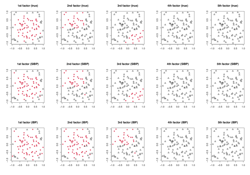
Figure 2: The true latent factors (top) and estimated factors by the proposed SIBP (middle) and the standard IBP (bottom).

Comparison of prediction performance

We next compare the performance of SIBP with other existing statistical or machine learning methods in estimating the underlying true multinomial probabilities, under situations where the exact spatial factors do not necessarily exist. We consider $M=50$ dimensional multinomial observations (five items for each dimension) for $i=1,\ldots,n$, where each observation is equipped with location information uniformly distributed on $[-1,1]\times[-1,1]$. For the true multinomial probabilities, we consider the following two scenarios in addition to Scenario (I) given in the previous section:

$${\rm(II)}\ \ \ \ z_{i1}=I(s_{i1}<0),\ \ \ \ z_{i2}=I(|s_{i2}|>s_{i1}),\ \ \ \ z_{i3}=I(s_{i1}>0.5,s_{i2}<-0.5),$$

$$\theta_{1ml}\sim N(1,3),\ \ \ \ \theta_{2ml}\sim N(0.5,(1.5)^{2})),\ \ \ \ \theta_{3ml}\sim t_{3}(2,1),$$

$${\rm(III)}\ \ \ \ z_{ilm}=I(s_{i2}>c_{lm}s_{i1}),\ \ \ c_{lm}\sim U(-2,2),\ \ \ \ \pi_{iml}\propto z_{ilm}s_{i1}+(1-z_{ilm})(s_{i1}^{2}+s_{i2}^{2}),$$

where $t_{m}(a,b)$ denotes the $t$-distribution with $m$-degrees of freedom having location and scale parameters, $a$ and $b$, respectively. Note that the multinomial probabilities in Scenario (III) are expressed as a function of the two-dimensional location information. The whole region is divided into two sub-regions with different underlying structures of multinomial probabilities.

Based on the observations on $n$ locations, we predict the multinomial probabilities in $n_{\rm test}$ locations. Let $\pi_{n+i,ml}$ be the true multinomial probability at the $i$th test location and $l$th category in the $m$th feature, and $\hat{\pi}_{iml}$ be the estimated one. The prediction performance is evaluated by the total mean squared errors (MSE), $(n_{\rm test}M)^{-1}\sum_{i=n+1}^{n+n_{\rm test}}\sum_{m=1}^{M}\sum_{l=1}^{c_{m}}(\hat{\pi}_{iml}-\pi_{iml})^{2}$. In this simulation study, we considered $(n,n_{\rm test})=(50,20)$. In addition to SIBP and IBP, we consider the following methods as competitors:

• Extreme gradient boosting tree (XGB): Using location information $(s_{i1},s_{i2})$ as input and $x_{im}$ as output, we employ the extreme gradient boosting tree (XGB) using the R package “xgboost”, separately for $m=1,\ldots,M$.

• Multinomial Gaussian process (MGP): For each $m$, the multinomial probability $\pi_{iml}$ is modeled as

  $$\pi_{iml}=\frac{\exp(w_{iml})}{\sum_{l^{\prime}=1}^{L}\exp(w_{iml^{\prime}})},\ \ \ \ \ (w_{1ml},\ldots,w_{nml})\sim N(0,\tau^{-1}Q(\psi)),$$

  where $Q(\psi)$ is a correlation matrix with unknown parameter $\psi$.

The prediction MSE values are averaged over 20 replications, and the results are shown in Table 1. Overall, the proposed SIBP provides better prediction accuracy than the other models. In particular, IBP does not consider spatial dependence and cannot predict unobserved locations while accounting for local spatial features, while SIBP achieves more accurate predictions owing to the latent Gaussian process. On the other hand, while MGP can model spatial trends of multinomial probabilities for accurate predictions, it struggles to capture discontinuous structures in spatial trends, leading to SIBP achieving higher accuracy than MGP.

Table 1: The mean squared errors (MSE) of prediction in test samples, produced by SIBP, IBP, XGBoost (XGB) and multinomial Gaussian process models (MGP), averaged over 20 Monte Carlo replications.

Scenario		SIBP	IBP	XGB	MGP
1		2.82	4.38	5.51	3.42
2		2.04	5.62	6.67	2.39
3		0.59	2.04	0.88	0.77

Applications

Spatial factor analysis of dialects

We here demonstrate the spatial factor models for multivariate multinomial data described in Section 3.4 using two real datasets regarding the geographical distributions of dialects observed in Fiji and Japan. In both cases, the observed data is an $n\times M$ matrix $X$ whose $(i,m)$-element $x_{im}$  ($i=1,\ldots,n$ and $m=1,\ldots,M$) takes one of $\{1,\ldots,c_{m}\}$, corresponding to $m$th feature in the $i$th area. Note that $c_{m}$ is the total number of features among $n$ areas. Analyzing this type of dataset is substantial in dialectology, and several statistical approaches such as network models (Lee and Hasegawa, 2011; Saitou and Jinam, 2017) and latent Dirichlet allocation (Syrjänen et al., 2016; Cathcart, 2020). Further, Murawaki (2020) developed a geographical factor model similar to the model in Section 3.4, with different probabilistic models for the latent binary variable and the number of factors being fixed. Here, we apply the spatial factor model with SIBP to two dialects data in Fiji and Japan to extract latent structures, including the number of factors.

Dialects in Fiji

For the dataset, $n=149$ (number of areas), $M=100$ (number of features), and $c_{m}$ ranges from $3$ to $35$, with the average value being $7.5$. We then applied the spatial factor models described in Section 3.4 with SIBP and $K=10$ (the largest number of factors) and the standard Gaussian process with an exponential kernel function. We generated 5000 posterior samples after discarding the first 5000 samples as a burn-in period. Based on the posterior samples, we computed the posterior probability being $z_{ik}=1$ and found that only a few areas are included in the 9th and 10th factors, so we regard the number of latent factors as 8. For each $k=1,\ldots,8$, we computed the posterior probability being $z_{ik}=1$ and show areas having a probability greater than 0.5 in Figure 3. It reveals that the geographical distribution of the detected factors varies significantly from one another, and the number of locations constituting each geographical factor decreases monotonically as the index of factors, which seems desirable for interoperability. Such property would come from the definition of the IBP that gives monotonically decreasing marginal prior probability having factors. Furthermore, except for Factor 2, the identified geographical factors exhibit geographically proximate structures, likely due to the influence of spatial correlation.

We also calculated the probabilities generating each word for each factor, where the results for selected 150 words are given in Figure 4. These results indicate that each factor maintains a distinct word distribution. Moreover, we visualized the factors present in each area in Figure 4. This result can be regarded as a clustering of areas represented by 8-bit encoding, making it possible to identify which locations share a common structure.

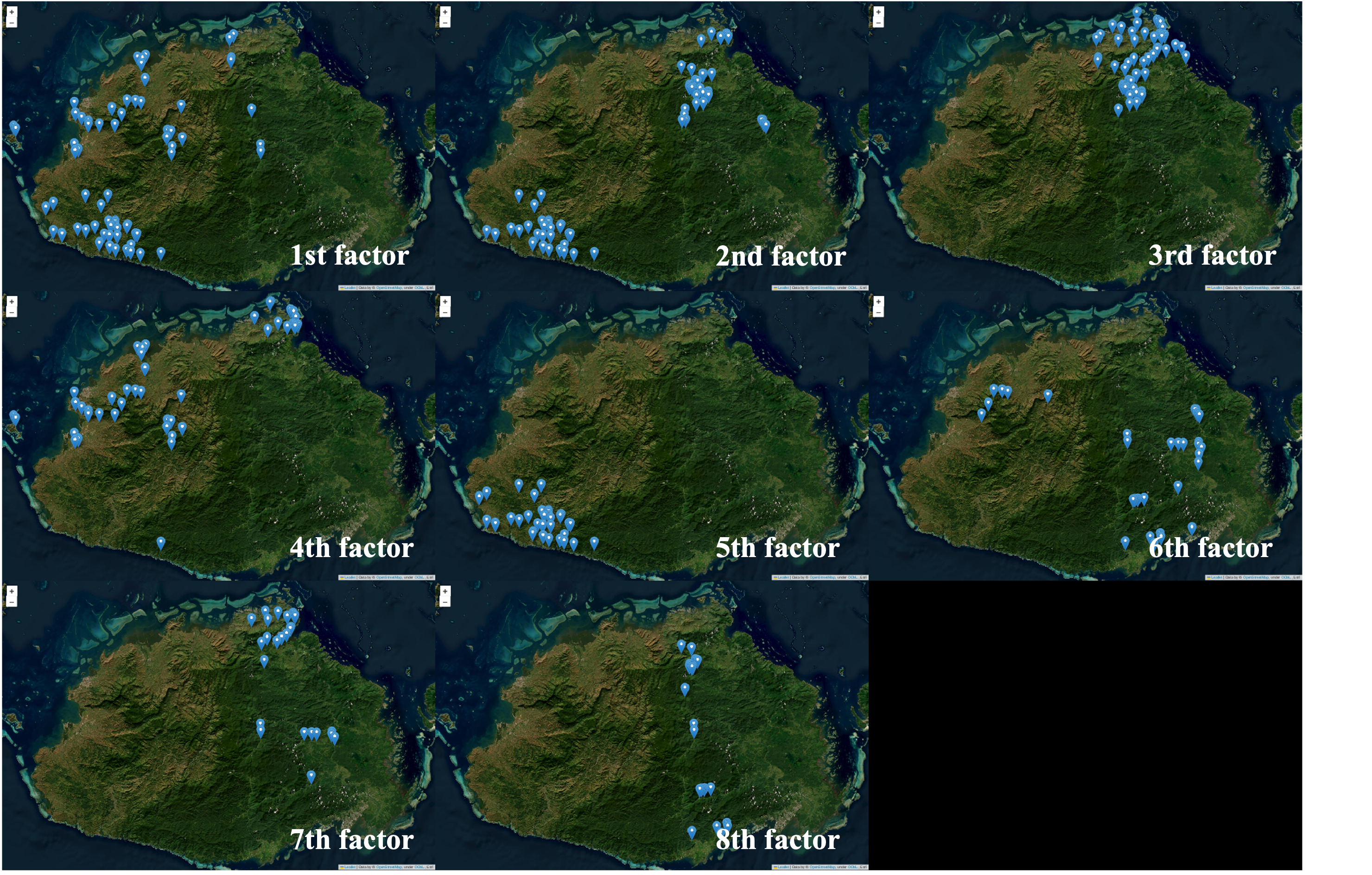
Figure 3: Detected non-null factors based on multinomial dialects data of 149 areas in Fiji.

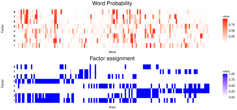
Figure 4: Posterior means of multinomial probabilities of selected 150 words for each factor, obtained by SIBP.

Dialects in Japan

We next apply a similar dialects dataset in Japan, which has $n=2317$ areas and $M=27$ features. Although there are approximately $5\%$ missing elements in the observed matrix $X$, it can be handled by our MCMC algorithm by imputing the missing values via data augmentation in each MCMC iteration. Since the number of areas is large, we apply the scalable version of the SIBP model with $K=10$ and $m=10$ nearest-neighbor Gaussian process, as described in Section 3.3. We generated 10000 posterior samples after discarding the first 5000 samples as burn-in. Since only two areas are included in the 10th factor, we regard the number of latent factors as 9. As in the previous application, we show the geographical distribution of detected factors in Figure 5, and word distributions and factors possessed by each area in Figure 6. As in the application to the data in Fiji, we can detect factors shared across different regions with variations in word distributions. Further, a 9-bit representation for each area in terms of the detected factors enables us to cluster areas with an understanding of commonalities between areas.

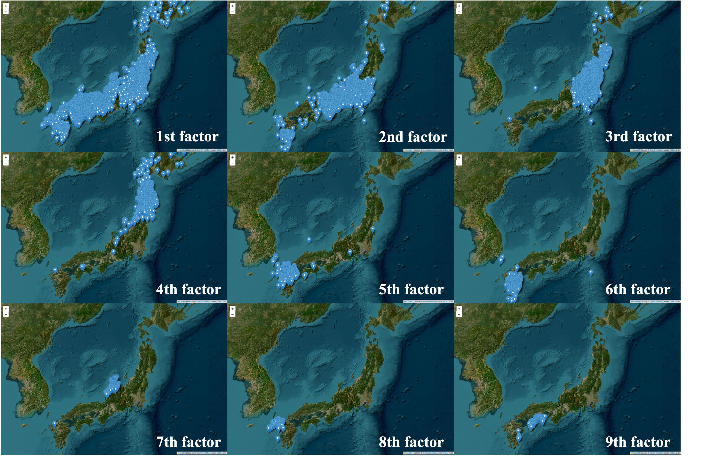
Figure 5: geographical distribution of detected factors by SIBP for Japan dialects data.

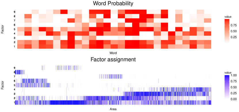
Figure 6: Multinomial probabilities of words for each factor (upper) and posterior probability of factor presence for each area (lower).

Factor analysis of geographical tree distribution

We next apply the SIBP model to tree census data in Japan reported in (Ishihara et al., 2011). The data is the number of trees (with girth at breast height of 15 cm or more) for each species, collected at 42 locations (typically one hector in each location), covering subarctic to subtropical climate zones and the four major forest types in Japan. By eliminating one outlying location and selecting tree species observed in at least 10 locations, the dataset we apply consists of $n=41$ locations and $M=45$ species.

We fit the multivariate count factor model described in Section 3.5 with SIBP and IBP. For SIBP, the standard Gaussian process with the exponential kernel is used, and the maximum number of factors is set to $K=7$ for both models. By generating 5000 posterior samples after discarding the first 5000 samples as burn-in, we calculated the posterior probability of the possession of factors. We detected four non-empty factors by SIBP and three non-empty factors by IBP. In Figure 7, we show the geographical distribution of the posterior probability of factor presence, which shows that IBP does not provide meaningful factors since 1st and 3rd factors exist in almost all the locations. On the other hand, four factors detected by SIBP seem to have different roles, as the geographical distribution of the posterior probabilities is quite different. Further, deviance information criteria (Spiegelhalter et al., 2002) is 5769 for SIBP and 6113 for IBP, showing the superior fitting of SIBP to IBP for this dataset. In Figure 8, we show each factor’s estimated log-intensity of $M=45$ species, indicating that the four factors have different characteristics. Finally, leveraging the latent Gaussian process, we predicted the probabilities of factor presence at arbitrary locations, which cannot be done without process-based spatial modeling. In Figure 9, we present the estimated probability of factor presence. It enables us to not only understand the continuous spatial variation in the probability of presence of each factor, but we can also predict at unobserved locations by combining the log-intensity of each factor as shown in Figure 8.

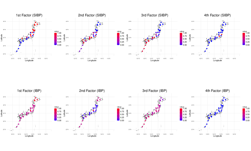
Figure 7: Geographical distribution of posterior probabilities of the presence of four factors, obtained by SIBP (upper) and IBP (lower).

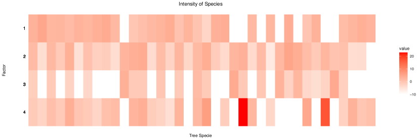
Figure 8: Posterior means of log-intensity of each species in four factors, obtained by SIBP.

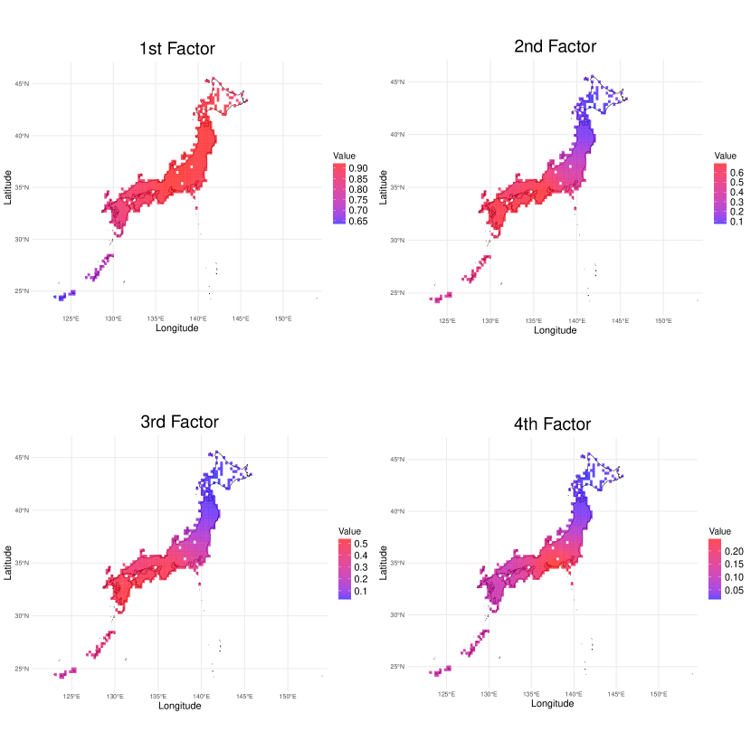
Figure 9: Predicted probability of the presence of the four factors, obtained by SIBP.

Concluding Remarks

We proposed SIBP, a generalization of the standard IBP, by incorporating spatial information through a latent Gaussian process. While we focus on two-dimensional spatial information, it can be immediately extended to general covariates; that is, two subjects with similar covariates tend to share the same factors. Such generalization would be useful in general latent feature (factor) models such as item response theory models (Li et al., 2023). Further, the proposed SIBP is worth developing its spatio-temporal version. Fast computation algorithm using, for example, variational approximation as done in Doshi et al. (2009) for the standard IBP. A detailed investigation would extend the scope of this paper, so that is left to future studies.

Appendix: Proofs of Propositions

A1. Proof of Proposition 1

Since $u_{i1},\ldots,u_{ik}$ are independent and their marginal distributions are $N(\mu,\tau^{-1})$, it follows that

$$P(z_{ik}=1)=E[z_{ik}]=E\left[\prod_{j=1}^{k}\sigma(u_{ij})\right]=\delta_{1}^{k}.$$

Since $\sigma(\cdot)$ is a logistic function, $\delta_{1}\in(0,1)$, so that we have $P(z_{ik}=1)\to 0$ as $k\to\infty$. Using the above results, we also have

$$E[c_{i}]=\sum_{j=1}^{k}E[z_{ij}]=\sum_{j=1}^{k}\delta_{1}^{j}=\delta_{1}\cdot\frac{1-\delta_{1}^{k}}{1-\delta_{1}}\to\frac{\delta_{1}}{1-\delta_{1}}>0$$

as $k\to\infty$. Furthermore, letting $u_{i}=(u_{i1},\ldots,u_{iK})$, we have

$${\rm Var}\left(c_{i}\right) ={\rm Var}\big{(}E[c_{i}|u_{i}]\big{)}+E\big{[}{\rm Var}(c_{i}|u_{i})\big{]}$$

$$={\rm Var}\left(\sum_{k=1}^{K}b_{ik}\right)+\sum_{k=1}^{K}E\left[b_{ik}(1-b_{ik})\right]$$

$$=E\left[\Big{(}\sum_{k=1}^{K}b_{ik}\Big{)}^{2}\right]-\left\{\sum_{k=1}^{K}E[b_{ik}]\right\}^{2}+\sum_{k=1}^{K}E[b_{ik}]-\sum_{k=1}^{K}E[b_{ik}^{2}]$$

$$=2\sum_{j=1}^{K}\sum_{k=1}^{j-1}E[b_{ij}b_{ik}]-\left\{\sum_{k=1}^{K}E[b_{ik}]\right\}^{2}+\sum_{k=1}^{K}E[b_{ik}]$$

where we used conditional independence of $z_{i1},\ldots,z_{iK}$ given $u_{i}$. Note that $E[b_{ik}]=C_{1}^{k}$ and $E[b_{ij}b_{ik}]=\delta_{2}^{k}\delta_{1}^{j-k}$ for $k<j$, Then, it follows that

$$\sum_{j=1}^{K}\sum_{k=1}^{j-1}E[b_{ij}b_{ik}] =\sum_{j=1}^{K}\delta_{1}^{j}\sum_{k=1}^{j-1}\left(\frac{\delta_{2}}{\delta_{1}}\right)^{k}$$

$$=\frac{\delta_{1}\delta_{2}}{\delta_{1}-\delta_{2}}\left(\frac{1-\delta_{1}^{K}}{1-\delta_{1}}-\frac{1-\delta_{2}^{K}}{1-\delta_{2}}\right)\to\frac{\delta_{1}\delta_{2}}{(1-\delta_{1})(1-\delta_{2})}$$

as $K\to\infty$. Hence, we have

$$\lim_{K\to\infty}{\rm Var}(c_{i}) =\frac{2\delta_{1}\delta_{2}}{(1-\delta_{1})(1-\delta_{2})}-\left(\frac{\delta_{1}}{1-\delta_{1}}\right)^{2}+\frac{\delta_{1}}{1-\delta_{1}}$$

$$=\frac{\delta_{1}}{1-\delta_{1}}\left(1+\frac{2\delta_{2}}{1-\delta_{2}}-\frac{\delta_{1}}{1-\delta_{1}}\right),$$

which completes the proof.

A2. Proof of Proposition 2

First, we note that

$$P(z_{ik}=1,z_{i^{\prime}k}=1)=E[b_{ik}b_{i^{\prime}k}]=\prod_{j=1}^{k}E[\sigma(u_{ij})\sigma(u_{i^{\prime}j})].$$

Without loss of generality, we assume that $\mu=0$ and $\tau=1$ in what follows. Since $(u_{ij},u_{i^{\prime}j})\sim N((0,0),R)$ with $R_{11}=R_{22}=1$, $R_{12}=R_{21}=\rho_{ii^{\prime}}$ and $\rho_{ii^{\prime}}=\rho(\|s_{i}-s_{i^{\prime}}\|;\psi)$, we have

$$D_{\mu,\tau}(\rho_{ii^{\prime}})\equiv E[\sigma(u_{ij})\sigma(u_{i^{\prime}j})]=\iint\sigma(x)\sigma(y)\phi_{2}((x,y);(0,0),R)dxdy,$$

where $\Sigma_{\tau}(\rho_{ii^{\prime}})$ is the $2\times 2$ covariance matrix, and this integral does not depend on $j$. We note that

$$\frac{\partial}{\partial\rho}\phi_{2}((x,y);(0,0),R) =\frac{\phi_{2}((x,y);(0,0),R)}{1-\rho^{2}}\left\{\rho+\frac{\rho}{1-\rho^{2}}(x^{2}-2\rho xy+y^{2})+xy\right\}$$

$$\geq xy\phi_{2}((x,y);(0,0),R),$$

for $\rho\in(0,1)$. Then, we have

$$\frac{\partial}{\partial\rho}D_{\mu,\tau}(\rho)\geq\iint xy\sigma(x)\sigma(y)\phi_{2}((x,y);(0,0),R)dxdy>0,$$

since $\rho_{ii^{\prime}}>0$ and $x\sigma(x)$ is an increasing function. Hence, the derivative $\partial D_{\mu,\tau}(\rho)/\partial\rho$ is positive for $\rho\in(0,1)$.

References

- Broderick et al. (2013) Broderick, T., J. Pitman, and M. I. Jordan (2013). Feature allocations, probability functions, and paintboxes. Bayesian Analysis 8(4), 801–836.
- Camerlenghi et al. (2024) Camerlenghi, F., S. Favaro, L. Masoero, and T. Broderick (2024). Scaled process priors for bayesian nonparametric estimation of the unseen genetic variation. Journal of the American Statistical Association 119(545), 320–331.
- Cathcart (2020) Cathcart, C. A. (2020). A probabilistic assessment of the indo–aryan inner–outer hypothesis. Journal of Historical Linguistics 10(1), 42–86.
- Datta et al. (2016) Datta, A., S. Banerjee, A. O. Finley, and A. E. Gelfand (2016). Hierarchical nearest-neighbor gaussian process models for large geostatistical datasets. Journal of the American Statistical Association 111(514), 800–812.
- Di Benedetto et al. (2020) Di Benedetto, G., F. Caron, and Y. W. Teh (2020). Non-exchangeable feature allocation models with sublinear growth of the feature sizes. In International Conference on Artificial Intelligence and Statistics, pp. 3208–3218. PMLR.
- Doshi et al. (2009) Doshi, F., K. Miller, J. Van Gael, and Y. W. Teh (2009). Variational inference for the indian buffet process. In Artificial Intelligence and Statistics, pp. 137–144. PMLR.
- Gershman et al. (2014) Gershman, S. J., P. I. Frazier, and D. M. Blei (2014). Distance dependent infinite latent feature models. IEEE transactions on pattern analysis and machine intelligence 37(2), 334–345.
- Grazian (2024) Grazian, C. (2024). Spatio-temporal stick-breaking process. Bayesian Analysis 1(1), 1–32.
- Griffiths and Ghahramani (2005) Griffiths, T. L. and Z. Ghahramani (2005). Infinite latent feature models and the indian buffet process. Technical Report GCNU TR 2005-001, Gatsby Computational Neuroscience Unit Technical Report.
- Griffiths and Ghahramani (2011) Griffiths, T. L. and Z. Ghahramani (2011). The indian buffet process: An introduction and review. Journal of Machine Learning Research 12(4).
- Ishihara et al. (2011) Ishihara, M. I., S. N. Suzuki, M. Nakamura, T. Enoki, A. Fujiwara, T. Hiura, K. Homma, D. Hoshino, K. Hoshizaki, H. Ida, et al. (2011). Forest stand structure, composition, and dynamics in 34 sites over japan. Ecological Research 26(6), 1007.
- Lee and Hasegawa (2011) Lee, S. and T. Hasegawa (2011). Bayesian phylogenetic analysis supports an agricultural origin of japonic languages. Proceedings of the Royal Society B: Biological Sciences 278(1725), 3662–3669.
- Li et al. (2023) Li, J., R. Gibbons, and V. Rockova (2023). Sparse bayesian multidimensional item response theory. arXiv preprint arXiv:2310.17820.
- Murawaki (2020) Murawaki, Y. (2020). Latent geographical factors for analyzing the evolution of dialects in contact. In Proceedings of the 2020 Conference on Empirical Methods in Natural Language Processing (EMNLP), pp. 959–976.
- Petralia et al. (2012) Petralia, F., V. Rao, and D. Dunson (2012). Repulsive mixtures. Advances in neural information processing systems 25.
- Polson et al. (2013) Polson, N. G., J. G. Scott, and J. Windle (2013). Bayesian inference for logistic models using pólya–gamma latent variables. Journal of the American statistical Association 108(504), 1339–1349.
- Ren et al. (2011) Ren, L., L. Du, L. Carin, and D. B. Dunson (2011). Logistic stick-breaking process. Journal of Machine Learning Research 12(1).
- Rodríguez et al. (2010) Rodríguez, A., D. B. Dunson, and A. E. Gelfand (2010). Latent stick-breaking processes. Journal of the American Statistical Association 105(490), 647–659.
- Saitou and Jinam (2017) Saitou, N. and T. A. Jinam (2017). Language diversity of the japanese archipelago and its relationship with human dna diversity. Man in India 97(1), 205–228.
- Spiegelhalter et al. (2002) Spiegelhalter, D. J., N. G. Best, B. P. Carlin, and A. Van Der Linde (2002). Bayesian measures of model complexity and fit. Journal of the royal statistical society: Series b (statistical methodology) 64(4), 583–639.
- Stolf and Dunson (2024) Stolf, F. and D. B. Dunson (2024). Allowing growing dimensional binary outcomes via the multivariate probit indian buffet process. arXiv preprint arXiv:2402.13384.
- Syrjänen et al. (2016) Syrjänen, K., T. Honkola, J. Lehtinen, A. Leino, and O. Vesakoski (2016). Applying population genetic approaches within languages: Finnish dialects as linguistic populations. Language Dynamics and Change 6(2), 235–283.
- Teh et al. (2007) Teh, Y. W., D. Grür, and Z. Ghahramani (2007). Stick-breaking construction for the indian buffet process. In Artificial intelligence and statistics, pp. 556–563. PMLR.
- Warr et al. (2022) Warr, R. L., D. B. Dahl, J. M. Meyer, and A. Lui (2022). The attraction indian buffet distribution. Bayesian Analysis 17(3), 931–967.
- Williamson et al. (2010) Williamson, S., P. Orbanz, and Z. Ghahramani (2010). Dependent indian buffet processes. In Proceedings of the thirteenth international conference on artificial intelligence and statistics, pp. 924–931. JMLR Workshop and Conference Proceedings.
- Xie and Xu (2020) Xie, F. and Y. Xu (2020). Bayesian repulsive gaussian mixture model. Journal of the American Statistical Association 115(529), 187–203.