Abstract

Primordial black holes (PBHs) may have formed through the gravitational collapse of cosmological perturbations that were generated and stretched during the inflationary era, later entering the cosmological horizon during the decelerating phase, if their amplitudes were sufficiently large. In this article, I will briefly introduce the basic concept of PBHs and review the formation dynamics through this mechanism, the estimation of the initial spins of PBHs and the time evolution of type II fluctuations, with a focus on the radiation-dominated and (early) matter-dominated phases.

1 1 0 https://doi.org/ Primordial black holes: formation, spin and type II Primordial black holes: formation, spin and type II Tomohiro Harada ¹ Tomohiro Harada Harada, T. Correspondence: harada@rikkyo.ac.jp

1 Introduction

Black holes may have formed in the early Universe. This possibility was first considered by Zel’dovich and Novikov (1966) Zel’dovich and Novikov (1967) and Hawking (1971) Hawking (1971). These black holes have been termed primordial black holes (PBHs). The observational relevance of PBHs to cosmology has been established by the subsequent work of Carr and Hawking (1974) Carr and Hawking (1974) and Carr (1975) Carr (1975).

The motivation for PBH research is multi-faceted. Since PBHs can, in principle, be observed, they provide valuable information about the early Universe. In this sense, PBHs can be regarded as the fossils of the early Universe. Furthermore, they are also one of the most promising candidates for dark matter. Moreover, Hawking evaporation plays an important role in the study of PBHs. Hawking recognised PBHs as a unique laboratory for studying black hole evaporation when he discovered this phenomenon in 1974 Hawking (1974, 1975). Hawking evaporation is key to understanding quantum gravity, where the information loss problem has been extensively discussed. The details of this evaporation may depend on quantum gravity and high-energy physics. PBHs are also important candidates for gravitational wave sources. Recently, several gravitational wave observatories have become available as observational tools to study strongly gravitating but otherwise dark objects, following LIGO’s first direct detection of gravitational waves in 2015 Abbott et al. (2016). It has been realised that gravitational waves provide a unique means of probing PBHs. This suggests that PBHs lie at the intersection of various growing fields of modern physics, such as cosmology, general relativity, gravitational waves, quantum gravity, and high-energy physics.

As observational data accumulate, gravitational waves are becoming an increasingly important means of observing our Universe. More than 100 events have been observed by the LIGO-Virgo-KAGRA (LVK) collaboration, and many of these have been identified as binary black holes. Several groups proposed the possibility that these binary black holes may be of cosmological origin, as many of them are approximately 30 $M_{\odot}$, which is more massive than was typically expected based on the standard theory of stellar evolution before the direct observations Sasaki et al. (2016); Bird et al. (2016); Clesse and García-Bellido (2017). As more observational data accumulate, information about not only the masses but also the spins of binary black holes is obtained for some events Abbott et al. (2017), which may provide a new clue to the origin of these binary black holes. From the obtained mass function of binary black holes, a search for the population of PBHs was carried out Franciolini et al. (2022). It has also been argued that the existence of subsolar candidates in LIGO data is a smoking gun for PBHs because no astrophysical scenario has yet been established to form subsolar-mass black holes Carr et al. (2024). Most recently, the NANOGrav collaboration reported evidence for nanohertz gravitational waves Agazie et al. (2023), which might be consistent with gravitational waves induced by scalar perturbations that could have produced the amount of PBHs responsible for the binary black holes observed by the LVK collaboration (e.g. Afzal et al. (2023)).

I would also comment on the possibility of PBHs constituting all or a considerable fraction of dark matter. We usually discuss this in terms of the fraction of PBHs to cold dark matter (CDM), $f(M)=\Omega_{\rm PBH}(M)/\Omega_{\rm CDM}$, as a function of the mass of PBHs, $M$. This fraction is observationally constrained very severely in some mass ranges but not in others. See Fig. 10 of Carr, Kohri, Sendouda and Yokoyama (2021) Carr et al. (2021) for an overview of the constraints. Recent observational constraints indicate two intriguing windows for dark matter. One is $M\sim 10^{17}-10^{23}$ g, where $f(M)$ is virtually unconstrained. This implies that PBHs could account for all the CDM for this mass range. The other mass range is $M\sim 1-10^{3}M_{\odot}$, where $f(M)\lesssim 0.1$, which is of interest in the context of terrestrial gravitational wave observations. In the latter range, however, a more recent paper has placed a new bound of $f\lesssim 10^{-3}$ for $M\sim 1-200M_{\odot}$ from LVK O3 data  Andrés-Carcasona et al. (2024).

Although there is currently a mass window in which all the CDM might be explained by PBHs, a stricter constraint could be placed on this mass window in the near future. Even if this turns out to be the case, it does not imply that studies of PBHs are without value. In this context, I would like to quote a profound statement by Bernard Carr: “Indeed their study may place interesting constraints on the physics relevant to these areas even if they never formed” Carr (2003).

2 Basic concept of primordial black holes

2.1 Mass

The striking feature of PBHs is that they can have a large range of possible mass scales from $10^{-5}$ g to $10^{56}$ g depending on the formation scenarios at least in principle. Although the mass of the PBH may depend on the scenario, we usually assume that it can be approximately given by the mass enclosed within the cosmological horizon or Hubble horizon at the formation time $t_{f}$ from the big bang as

$$M\simeq M_{H}(t_{f})\simeq\frac{c^{3}}{G}t_{f}\simeq 1M_{\odot}~{}\left(\frac{t_{f}}{10^{-5}~{}\mathrm{s}}\right),$$ (1)

where $c$ and $G$ are the speed of light and the gravitational constant, respectively, for which the gravitational radius is given by

$$R_{g}\simeq 1~{}\mathrm{km}~{}\left(\frac{M}{M_{\odot}}\right).$$ (2)

So, we can say “the smaller, the older”. Table 1 shows the relation between the formation time and the initial PBH mass. Nevertheless, we should keep a caveat in our mind that the mass of PBHs could be much smaller than the horizon mass in certain formation scenarios.

Table 1: The cosmological time and the initial mass of PBHs if they are formed then

Cosmological time	Mass of PBHs
$\sim 10^{-43}$ s [Planck time]	$\sim 10^{-5}$ g [Planck mass]
$\sim 10^{-23}$ s	$\sim 10^{15}$ g [Critical Mass]
$\sim 10^{-5}$ s [QCD crossover]	$\sim 10^{33}$ g [Solar mass]
$\sim 10^{12}$ s [Matter-radiation equality]	$\sim 10^{50}$ g
$\sim 10^{19}$ s [Present epoch]	$\sim 10^{56}$ g [Mass of the observable Universe]

It is nontrivial that how the initial mass of PBHs is related to the mass during their evolution. As for the mass accretion, earlier works suggest that it does not so significantly affect the mass at least in radiation domination Carr and Hawking (1974). This was confirmed by numerical simulations (e.g. Escrivà (2020)). On the other hand, the Hawking evaporation is considered to decrease the mass of PBHs. The mass loss is considered to virtually be negligible if the mass of the PBH is much more massive than the critical mass $\sim 10^{15}$ g, which will be discussed below.

2.2 Evaporation

Based on quantum field theory in curved spacetimes, Hawking (1974) Hawking (1974, 1975) found that black holes emit black body radiation. The temperature $T_{H}$ of the black body, which is called the Hawking temperature, is proportional to the surface gravity of the horizon and is given for the Schwarzschild black hole by

$$T_{H}=\frac{\hbar c^{3}}{8\pi GMk}\simeq 100~{}\mathrm{MeV}~{}\left(\frac{M}{10^{15}\mathrm{g}}\right)^{-1},$$ (3)

where $\hbar$ and $k$ are the reduced Planck constant and the Boltzmann constant, respectively. This is called the Hawking evaporation. If we assume that the black hole loses its mass due to this radiation of quantum fields, which is the so-called semi-classical approximation, we obtain

$$\frac{dM}{dt}=-\frac{g_{\rm eff}\hbar c^{4}}{15360\pi G^{2}M^{2}},$$ (4)

where $g_{\rm eff}\sim 100$ is the effective degrees of freedom and the grey-body factor is neglected. This implies that the evaporation timescale $t_{\rm ev}$ is given by

$$t_{\rm ev}\simeq\frac{G^{2}M^{3}}{g_{\rm eff}\hbar c^{4}}\simeq 10~{}\mbox{Gyr}\left(\frac{M}{10^{15}\mbox{g}}\right)^{3},$$ (5)

after which the black hole of mass $M$ loses almost all of its mass. As the black hole decreases its mass, the temperate gets higher and higher and the evaporation timescale becomes shorter and shorter. Although the black hole decreases its mass very slowly in most of its life, it rapidly loses its remaining mass at its final moment, which is called a black hole explosion. When it becomes as light as the Planck mass $m_{\rm Pl}\sim 10^{-5}$ g, the semi-classical approximation necessarily breaks down and the subsequent evolution of the black hole should greatly depend on quantum gravity.

From Eq. (5), the critical mass is approximately given by $10^{15}$ g for which $t_{\rm ev}=t_{0}$ is satisfied, where $t_{0}$ is the age of the Universe. So, if $M\lesssim 10^{15}$ g, PBHs have dried up after the explosion until now, whether they leave Planck mass relics or not. If $M\sim 10^{15}$ g, PBHs are currently emitting X rays and $\gamma$ rays and can be observed through those emissions. If $M\gtrsim 10^{17}$ g, the evaporation is mostly negligible and the mass of the PBH remains almost constant until now.

2.3 Probability

To discuss the formation, the fraction $\beta(M)$ of the Universe which goes into PBHs when the mass contained within the cosmological horizon is $M$, is often used. This can also be regarded as the formation probability of PBHs. If we consider PBHs formed in the radiation-dominated phase, PBHs act as nonrelativistic particles surrounded by relativistic particles. Therefore, the energy density of PBHs, $\rho_{\rm PBH}$, decays as $a^{-3}$, while the energy density of relativistic particles, $\rho_{\rm rad}$, decays as $a^{-4}$, where $a$ is the scale factor of the Universe. As a result, $\beta(M)$ is not equal to the current fraction of PBHs of mass $M$ to all the CDM, which is given by

$$f(M)=\left.\frac{\Omega_{\rm PBH}}{\Omega_{\rm CDM}}\right|_{t=t_{0}}.$$ (6)

Taking in account the effect that PBHs are concentrated during the radiation-dominated era, we find

$$\beta(M) \simeq 2\times 10^{-18}\left(\frac{M}{10^{15}~{}\mathrm{g}}\right)^{1/2}f(M)$$ (7)

for $M\gtrsim 10^{15}$ g. Thus, only a tiny probability $\beta\simeq 2\times 10^{-17}$ is enough to explain all of the dark matter if $M=10^{17}$ g.

For $M\gtrsim 10^{15}$ g, Eq. (7) combined with the observational constraint on $f(M)$ gives the observational constraint on $\beta(M)$. As for $M\lesssim 10^{15}$ g, PBHs have evaporated away until now. However, the evaporation of PBHs may spoil big bang nucleosynthesis for $M\sim 10^{10}-10^{13}$ g if $\beta(M)$ is too large. Such a consideration gives the observational constraint on $\beta(M)$ for $M\gtrsim 10^{-5}$ g, where the lower limit is usually assumed to be the Planck mass. See Fig. 18 of Ref. Carr et al. (2021) for more details.

3 Formation

3.1 Overview

The serious study of PBH formation date back to Carr (1975) Carr (1975). One of its aims is to theoretically predict $\beta(M)$ and therefore $f(M)$ and other observables of PBHs for a given cosmological scenario. We can obtain the information of the early Universe from observational data on PBHs only through these studies. Apart from such an observational motivation, through the study of formation we can understand physics in PBH formation and investigate new phenomena and/or new physics in highly nonlinear general relativistic dynamics and high-energy physics. There have been a lot of scenarios proposed for PBH formation. One of the most standard ones is the direct collapse of a large amplitude of primordial perturbations generated by inflation. This can be considered as ‘inevitable’ as the inflationary cosmology has been regarded as an essential part of standard cosmology. Among the other alternative scenarios, domain wall collapse, bubble nucleation, collapse of string networks and phase transitions have attracted more attention than others. Hereafter, we will focus on the formation scenario from fluctuations generated by inflation. Studies on this scenario have developed more than on other scenarios. The key ideas to this scenario is the following: fluctuations generated by inflation, long-wavelength solutions, formation threshold, black hole critical behaviour, dependence on the equation of state (EOS) and statistics on the abundance estimate. We will briefly view these topics below.

3.2 Fluctuations generated by inflation

The most striking feature of inflation is that it can not only solve the flatness problem and the horizon problem but also provide the mechanism to generate fluctuations as quantum effects. Those fluctuations seed structure formation of different scales in our Universe and provide anisotropy in cosmic microwave background (CMB) currently observed with high accuracy.

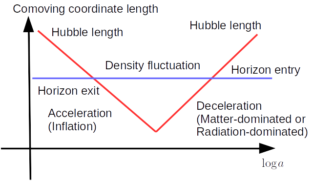
Figure 1: Evolution of the scale of fluctuations after generated by inflation

The evolution of fluctuations in the inflationary cosmology is schematically illustrated in Fig. 1. The quantum fluctuations generated by inflation are stretched to the length scales much larger than the Hubble horizon scale $cH^{-1}$ because the fluctuation scale, which is proportional to $a$, expands faster than the Hubble horizon scale, which is proportional to $t$, due to the accelerated expansion. This process is also considered to lose quantum coherence from the fluctuations. The generated classical fluctuations are further stretched away compared to the Hubble length as long as the inflationary phase continues. After the inflation ends, the expansion of the Universe begins to be decelerated. There is a possibility that the Universe might experience the early matter-dominated phase due to the harmonic oscillation of an inflaton field. In any case, the Universe eventually gets dominated by the radiation field, the tightly coupled relativistic particles in an almost complete thermal equilibrium state. This process is called reheating. If we consider the scale of the fluctuation much larger than the Hubble horizon in the decelerated Universe, the scale of the fluctuation, which is proportional to $a$, expands slower than the Hubble horizon scale, which is proportional to $t$. The time when the fluctuation scale gets as large as the Hubble scale is called the horizon entry of the perturbation. Although the inflationary cosmology has been becoming an essential part of the standard cosmology, there has been no standard inflation model until now. There are lots of inflation models, each of which gives the power spectrum $P_{\zeta}(k)$ and the other statistics of the curvature perturbations $\zeta$. See Ref. Sasaki et al. (2018) for details of different inflation models in the context of PBH formation.

3.3 Large-amplitude long-wavelength solutions

As discussed above, the scale of fluctuation generated by inflation gets much larger than the Hubble horizon scale. Therefore, after inflation ends, we have the fluctuations of super-horizon scales in the decelerated expansion. In this phase, we can construct the so-called long-wavelength solutions of the Einstein equation Tomita (1972); Shibata and Sasaki (1999); Lyth et al. (2005); Polnarev and Musco (2007).

Figure 2: Schematic figure of long-wavelength solutions

In order to discuss the PBH formation in radiation domination, it is necessary to deal with a nonlinearly large amplitude of perturbation. We implement gradient expansion of the Einstein equation to obtain the long-wavelength solutions, where the spatial derivative is regarded as much smaller than the time derivative. More precisely, we take the following procedure Shibata and Sasaki (1999); Harada et al. (2015). We first decompose the metric to the following $3+1$ form:

$$ds^{2}=-\alpha^{2}dt^{2}+e^{2\zeta}a^{2}(t)\tilde{\gamma}_{ij}(dx^{i}+\beta^{i}dt)(dx^{j}+\beta^{j}dt),$$ (8)

where $i,j$ run over 1,2 and 3 and $\alpha$, $\beta^{i}$, $\tilde{\gamma}_{ij}$ and $\zeta$ are the functions of $t$ and $x^{i}$ and called the lapse function, the shift vector, the spatial metric and the curvature perturbation, respectively, while $a(t)$ is the scale factor of the reference Friedmann-Lemaître-Robertson-Walker (FLRW) spacetime. We require that $\det(\tilde{\gamma}_{ij})=\det(\eta_{ij})$, where $\eta_{ij}$ is the time-independent metric of the flat 3 space. Then, we assume that the scale of the perturbation is much larger than the Hubble horizon scale, i.e., that

$$\epsilon:=\frac{k}{aH}$$ (9)

is much smaller than unity. Applying the gradient expansion for the Einstein equation, we can obtain growing-mode solutions with an assumption that the zeroth order solutions in powers of $\epsilon$ takes the following form:

$$ds^{2}=-dt^{2}+e^{2\zeta_{0}({\bf x})}a^{2}(t)\eta_{ij}dx^{i}dx^{j}.$$ (10)

Note that this assumption is compatible with the comoving slice, the constant-mean-curvature slice and the uniform-density slice but not with the conformal Newtonian gauge condition, which is often used in cosmology. The higher-order terms of the solutions are obtained in terms of the function $\zeta_{0}({\bf x})$ if we impose the appropriate gauge conditions. In other words, $\zeta_{0}({\bf x})$, which is not suppressed due to the long-wavelength scheme, generates the long-wavelength solutions. For example, the density perturbation $\delta$ is $O(\epsilon^{2})$ and is given by

$$\delta_{\rm CMC}\simeq-\frac{4}{3a^{2}H^{2}}e^{-\frac{5\zeta_{0}}{2}}\Delta_{\rm flat}e^{\frac{\zeta_{0}}{2}}$$ (11)

in the constant-mean-curvature slice.

If we apply this formulation to the spherically symmetric spacetime, where the zeroth order metric can be written in the following form

$$ds^{2}=-dt^{2}+e^{2\zeta_{0}(r)}[dr^{2}+r^{2}(d\theta^{2}+\sin^{2}\theta d\phi^{2})],$$ (12)

in the conformally flat coordinates, we can show that this is equivalent to the asymptotically quasi-homogeneous solutions developed in Ref. Polnarev and Musco (2007) in the Misner-Sharp formulation, where the comoving slice and the comoving thread are adopted, and the explicit transformation between them is given in Ref. Harada et al. (2015).

3.4 Formation threshold in radiation domination

If the amplitude of the perturbation, which is generated by inflation and enters the horizon in the radiation-dominated era, is sufficiently large, it will directly collapse to a black hole. Since the linear perturbation in the radiation-dominated era does not grow, such a perturbation must be nonlinearly large. This prevents us from directly accessing the full dynamics of PBH formation with analytical methods. Only full numerical relativity simulations can accurately describe the general relativistic dynamics of PBH formation, which has been pioneered by Nadezhin, Novikov and Polnarev (1978) Nadezhin et al. (1978). In fact, it has been established by several analytical and numerical works of the Einstein equation that PBHs really form in this scenario.

This scenario naturally implies that there exists a threshold for PBH formation. Carr (1975) derived the threshold $\delta_{th}\sim 1/3$ for radiation domination according to the Jeans scale argument in terms of $\delta_{H}$, the density perturbation at the horizon entry of the perturbation. In numerical relativity, the threshold value is obtained as $\delta_{th}\sim 0.45$ in terms of the density perturbation averaged in the comoving slice over the Hubble patch at the horizon entry of the overdense region, where $\delta_{H}$ is regarded as that in the nontrivial lowest order of the long-wavelength expansion scheme Musco et al. (2005, 2009); Musco and Miller (2013); Harada et al. (2015). Harada, Yoo and Kohri (2013) Harada et al. (2013) refined Carr’s argument from a general relativistic point of view and analytically derived the threshold $\delta_{th}\simeq 0.41$ in the comoving slice. Although the averaged density perturbation $\delta_{H}$ might look straightforward to interpret, it has difficulty in its interpretation. This is because if we calculate the averaged density perturbation at the horizon entry using the nontrivial lowest order of the solutions, it cannot be a real physical value, as the latter can only be obtained after the full numerical simulation and is not necessarily useful.

Shibata and Sasaki (1999) Shibata and Sasaki (1999) defined a compaction function in the constant-mean curvature slice. Although it was intended to equal to the ratio of the excess in the Misner-Sharp mass, or equivalently the Kodama mass, to the areal radius, it is not equal to that but to

$${\cal C}_{\rm SS}:=\frac{1}{2}\left[1-\left(1+r\zeta^{\prime}\right)^{2}\right]$$ (13)

in the long-wavelength limit, where we omit the subscript $0$ in $\zeta$ according to the convention Harada et al. (2015, 2023). It is proportional to the ratio of the Misner-Sharp mass excess to the areal radius in the comoving slice as

$${\cal C}_{\rm SS}(r)\approx\frac{3}{4}C_{\rm com}(r),$$ (14)

where

$$C_{\rm com}:=\frac{2\delta M_{\rm com}}{R}$$ (15)

with $\delta M_{\rm com}$ being the Misner-Sharp mass excess in the comoving slice. Note the factor 2 on the right-hand side of Eq. (15). The threshold value is $\sim 0.4$ in terms of its maximum value of the Shibata-Sasaki compaction function ${\cal C}_{\rm SS}(r)$ in the long-wavelength limit Shibata and Sasaki (1999); Musco and Miller (2013); Harada et al. (2015). This is more straightforward than the averaged density perturbation because for the compaction function description, we only have to take the long-wavelength limit of the solutions, where all the higher-order contributions naturally disappear. This is probably why people have favoured to use the compaction function.

In the last decade, great effort has been paid to reveal the profile dependence of the threshold Nakama et al. (2014); Musco (2019); Escrivà et al. (2020). In particular, Escrivà, Sheth and Germani (2020) Escrivà et al. (2020) found a universal threshold

$$\bar{C}_{\rm com}\simeq\frac{2}{5}$$

in terms of $\bar{C}_{\rm com}$, the spatial average of $C_{\rm com}$ over $0<r<r_{m}$, where $C_{\rm com}(r)$ takes a maximum at $r=r_{m}$. This holds within $2\%$ accuracy over different profiles they surveyed. This gives a new threshold condition that uses the maximum $C_{\rm com}(r_{m})$ and the second derivative of $C^{\prime\prime}_{\rm com}(r_{m})$. See Ref. Escrivà et al. (2020) for details.

3.5 Softer equation of state

Although PBH formation has been conventionally studied in the radiation-dominated phase, the scenarios in other phases with effectively softer equations of state will also be important because the generation should be enhanced then. This scenario already was noticed in Carr (1975) Carr (1975), where the threshold density perturbation was estimated to $\delta_{H}\sim w$ for the linear EOS $p=w\rho$ using the simple application of the Jeans criterion in Newtonian gravity. Harada, Yoo and Kohri (2013) Harada et al. (2013) refined it by comparing the free-fall time and the sound-crossing time in a simplified model of the general relativistic spacetime considering gauge difference to find the threshold value

$$\delta_{H}\simeq\frac{3(1+w)}{5+3w}\sin^{2}\left(\frac{\pi\sqrt{w}}{1+3w}\right)$$ (16)

in the comoving slice. This analytical expression showed a good agreement with the results of numerical relativity simulation Musco and Miller (2013); Escrivà et al. (2021) for $0<w\leq 1/3$ as seen in Fig. 3. These studies showed that the threshold for the EOS $p=w\rho$ is an increasing function of $w$ for $0<w\leq 1/3$ and approaches 0 as $w\to 0$. For example, for the QCD crossover, for which $w$ drops to $\sim 0.23$ from $1/3$ Byrnes et al. (2018), the PBH formation will be enhanced by a factor of the order of 1000 Escrivà et al. (2023); Musco et al. (2024).

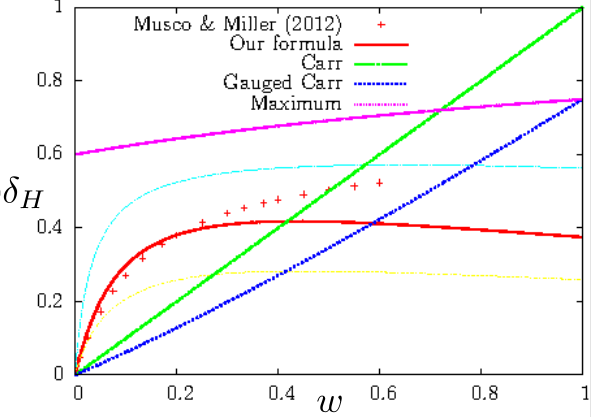
Figure 3: EOS dependence of the PBH formation threshold. See also Ref. Harada et al. (2013).

3.6 Matter domination

If the argument in Sec. 3.5 for the EOS $p=w\rho$ applied to $w\approx 0$ for the matter-dominated phase, one might consider that PBHs could be overproduced. However, this cannot be correct because the realistic physical system is highly nonspherical and the deviation from spherical symmetry will grow during the collapse in matter domination. Not only after the standard matter-radiation equality time but also in a possible early matter-dominated phase, which may naturally occur in the preheating process or in the strong phase transition in the Universe, PBH formation will be enhanced. This is one of the interesting epochs to study in the context of PBH formation. Since the condition for PBH formation is not solely determined by the pressure gradient force, we would need a totally different treatment for this phase from that for the radiation-dominated phase.

The PBH formation in matter domination has been pioneered by Khlopov and Polnarev (1980) Khlopov and Polnarev (1980); Polnarev and Khlopov (1982), where the effects of anisotropy and inhomogeneity are studied as obstruction of PBH formation process. Harada, Yoo, Kohri, Nakao and Jhingan (2016) Harada et al. (2016) revisited the anisotropic effects by combining the picture of pancake collapse of dark matter and the hoop conjecture by Thorne, which claims that black holes with horizons form when and only when a mass $M$ gets compacted into a region whose circumference in every direction is ${\cal C}\lesssim 4\pi M$  Klauder (1972); Misner et al. (1973). This suppression due to the anisotropic effect is schematically shown in Fig. 4. They not only qualitatively reproduced the result of Ref. Khlopov and Polnarev (1980); Polnarev and Khlopov (1982) but also updated the coefficient as

$$\beta_{\rm aniso}\simeq 0.05556\sigma_{H}^{5},$$ (17)

where $\sigma_{H}$ is the standard deviation of $\delta_{H}$ and the Gaussian distribution for density perturbation is assumed.

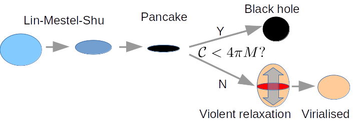
Figure 4: Schematic illustration of the anisotropic effect in the formation of PBHs in matter domination. ${\cal C}$ denotes the hoop of the surface the gravitating object of mass $M$. See Ref. Harada et al. (2016) for details.

Kopp, Hofmann and Weller (2010) Kopp et al. (2011) modelled spherical formation of PBHs in matter domination with the Lemaître-Tolman-Bondi (LTB) solution and Harada and Jhingan (2015) Harada and Jhingan (2016) extended it to nonspherical formation with the Szekeres quasi-spherical solutions. Kokubu, Kyutoku, Kohri and Harada (2018) Kokubu et al. (2018) revisited the inhomogeneity effects by utilising the LTB solution and not only qualitatively reproduced the result of Ref. Khlopov and Polnarev (1980); Polnarev and Khlopov (1982) but also updated the coefficient so that the additional suppression factor is given by

$$\beta_{\rm inhom}\simeq 3.70\sigma_{H}^{3/2}$$ (18)

with the caveat that its physical effect largely depends on the assumption that black hole formation is prevented by the appearance of an extremely high-density region before the black hole horizon formation surrounding it.

Harada, Kohri, Sasaki, Terada and Yoo (2022) Harada et al. (2023) showed that the effects of velocity dispersion that may have been generated in possible nonlinear growth of perturbation in the earlier phase can suppress PBH formation. The effects of the angular momentum can play important roles and suppress PBH formation for smaller $\sigma_{H}$ Harada et al. (2017). We will later discuss the angular momentum in the PBH formation in the matter-dominated era in the context of the initial spins of PBHs.

3.7 Critical behaviour

One of the great achievements of numerical relativity is the discovery of critical behaviour in gravitational collapse, which is also called black hole critical behaviour. This has been first discovered by Choptuik (1993) Choptuik (1993) in the spherically symmetric system of a massless scalar field and followed by Evans and Coleman (1994) Evans and Coleman (1994) in the spherical system of a radiation fluid. The phenomena were theoretically revealed in terms of the renormalisation group analysis by Koike, Hara and Adachi (1995) Koike et al. (1995). These early studies were all on asymptotically flat spacetimes and whether it applies also for PBH formation was not so trivial because of the different boundary conditions and the existence of the characteristic scale, the Hubble horizon length. The critical behaviour in the PBH formation was discovered by Niemeyer and Jedamzik (1999) Niemeyer and Jedamzik (1999) but subsequently questioned Hawke and Stewart (2002). Finally, Musco and Miller (2013) Musco and Miller (2013) beautifully confirmed the critical behaviour in PBH formation. The essence of the critical behaviour in the context of PBH formation is the following. Let us consider a one-parameter family of initial data, for which we can choose the averaged density perturbation $\delta_{H}$ as the parameter of the family. As we have already seen, there is a threshold value $\delta_{\rm th}$, beyond which a PBH forms. Then, the evolution of the initial data which has the critical value $\delta_{H}=\delta_{\rm th}$ approaches a particular member of continuously self-similar solutions, which is called a critical solution. If $\delta_{H}$ is slightly above the critical value, we have PBH formation and the scaling law for the mass of the formed PBH, $M$, holds as follows:

$$M\approx KM_{H}(\delta_{H}-\delta_{\rm th})^{\gamma},$$ (19)

where $K$ is a positive constant of the order of the unity and $\gamma\simeq 0.36$ is called a critical exponent. In fact, the critical behaviour, such as the critical solution and the critical exponent, does not depend on the choice of the one-parameter family of initial data, which is called universality. Note, however, that the critical solution and the critical exponent do depend on the matter field and the equation of state even if it is a perfect fluid Maison (1996).

In the context of PBH formation, if we assume that $\delta_{H}$ obeys some reasonable statistical distribution, the critical behaviour implies that only a tiny fraction of perturbations of mass scale $M_{H}$ can be much smaller than $M_{H}$, while a large fraction remain of the order of $M_{H}$. This becomes important especially if we consider $\beta(M)$ for $M\sim 10^{16}-10^{17}$ g. This is because the PBHs of the critical mass $\sim 10^{15}$ g are severely constrained by observation through its X-ray or gamma-ray emission, while those of $\sim 10^{16}-10^{17}$ g are not. For example, the formation probability $\beta(M)$ with the horizon mass $M=10^{16}$ g is severely constrained by such a tiny fraction of PBHs of the critical mass $\sim 10^{15}$ g considerably smaller than $10^{16}$ g Niemeyer and Jedamzik (1998); Yokoyama (1998).

3.8 Abundance estimation and statistics

Even if we can identify the threshold condition and the classical dynamics of PBH formation and subsequent evolution, it is not sufficient to determine $\beta(M)$. Clearly, we also need statistical properties of the perturbations. In inflationary cosmology, the statistical properties of fluctuations generated by inflation, such as the power spectrum $P_{\zeta}(k)$ and other statistical properties, can be predicted at least in principle if we fix the inflation model.

Carr (1975) Carr (1975) simply assumed that $\delta_{H}$ obeys a Gaussian distribution and obtained the following formula

$$\beta\simeq 2\frac{1}{\sqrt{2\pi}\sigma_{H}}\int^{\delta_{\rm max}}_{\delta_{\rm th}}d\delta e^{-\frac{\delta^{2}}{2\sigma_{H}^{2}}}\simeq\sqrt{\frac{2}{\pi}}\frac{\sigma_{H}}{\delta_{\rm th}}e^{-\frac{\delta_{\rm th}^{2}}{2\sigma_{H}^{2}}},$$ (20)

where $\delta_{\rm max}$ and $\sigma_{H}$ are the possible maximum value and the standard deviation of $\delta_{H}$ and in the last approximation $\delta_{\rm th}\gg\sigma_{H}$ is assumed. Since we need at least $\beta(M)\gtrsim 10^{-18}$ for PBHs to contribute to a considerable fraction of dark matter, we can conclude that only the Gaussian tail beyond $\sim 8\sigma_{H}$ is responsible for PBHs, which is shown in Fig. 5. This implies that introducing even small non-Gaussianity can significantly enhance the formation of PBHs Young and Byrnes (2013).

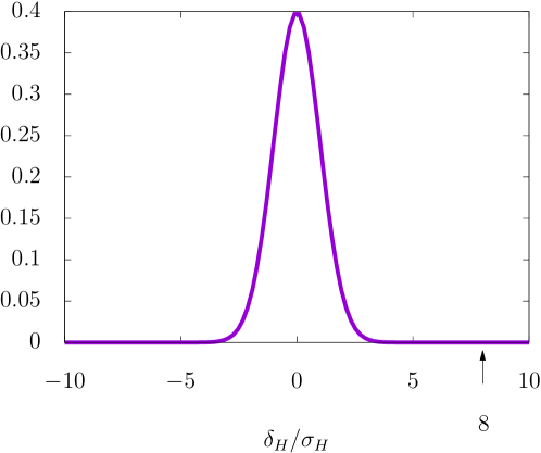
Figure 5: Gaussian distribution of the averaged density perturbation $\delta_{H}$. Only the tail beyond $\sim 8\sigma_{H}$ is responsible for PBHs for the typical case.

If we consider PBHs formed in the radiation-dominated era and assume $\delta_{\rm th}\simeq 0.45$, we need at least $\sigma_{H}\gtrsim 0.05$ or $P_{\zeta}(k)\gtrsim 0.01$. This is much larger than the observed value $P_{\zeta}(k)\simeq 10^{-10}$ for the CMB anisotropy, although it does not immediately exclude the considerable formation of PBHs because the scales of the PBHs and the CMB anisotropies are usually very different from each other.

Although Carr’s formula (20), which is also called the Press-Schechter approximation, is very useful, this is considered as a very rough approximation. One of the reasons is that even if the curvature perturbation obeys a Gaussian distribution, the averaged density perturbation $\delta_{H}$ in the comoving slice cannot because it must be within a finite interval between the minimum $-1$ and the maximum $2/3$ Kopp et al. (2011). The other is that since PBHs will form only at very rare peaks of the perturbation, peak theory should apply, which is known to give a physically reasonable prediction for galaxy formation Bardeen et al. (1986). The prediction of peak theory may be significantly different from that of Carr’s formula for the estimation of PBH abundance. Currently, there are a few variations in the application of peak theory to the estimation of the PBH abundance, which comes from theoretical ambiguity caused by incomplete understanding of nonlinear, nonspherical and multi-scale general relativistic dynamics Yoo et al. (2018, 2021); Germani and Sheth (2020, 2023).

4 Initial spins

If the black hole no hair conjecture holds in astrophysics, stationary black holes in vacuum should be well approximated by Kerr black holes which are characterised only by two parameters, the mass and the angular momentum. As we have already discussed, the mass of PBHs is approximately equal to that within the Hubble horizon at the time of formation. So, what determines the spin of PBHs? If black holes of masses from several to several tens of solar masses are observed, it would be very difficult to distinguish between PBHs and astrophysical black holes. Astrophysical black holes form in the final stage of evolution of massive stars. If we observe an isolated black hole, the only information of its own other than its mass is its spin. So, if the spins of PBHs are expected to be very different from those of astrophysical black holes, the observation of spin can be potentially decisive information to distinguish between the two populations. Here, we focus on the initial spins of PBHs, although the accretion and merger history after their formation may also greatly affect their spins depending on the scenarios De Luca et al. (2020).

4.1 Spins of primordial black holes formed in radiation domination

It was discussed that the formation process of PBHs in radiation domination is well approximated by spherically symmetric dynamics since Carr (1975) Carr (1975). Recent quantitative studies have revealed that this early argument is basically correct. The key of the quantitative analysis is peak theory.

For PBHs formed in radiation domination, the threshold density perturbation $\delta_{\rm th}$ is of the order of the unity, which is considerably larger than its standard deviation. In other words, PBHs can form only at very rare peaks. Peak theory predicts that there is only very small deviation from spherical symmetry for such rare peaks. This is very important to not only justify spherical symmetry assumption but also estimate the angular momentum of PBHs formed in radiation domination. Based on the perturbative analysis based on peak theory, De Luca, Desjacques, Franciolini, Malhotra and Riotto (2019) De Luca et al. (2019) concluded that the root mean square of the nondimensional Kerr parameter $a_{*}$ is of the order of $10^{-2}$, while Harada, Yoo, Kohri, Koga and Monobe (2021) estimated the root mean square of $a_{*}$ to be of the order of $10^{-3}$ and showed that a small fraction of PBHs of masses much smaller than the mass enclosed within the Hubble horizon, $M\ll M_{H}$, as a result of critical phenomena, can have much larger spins Harada et al. (2021).

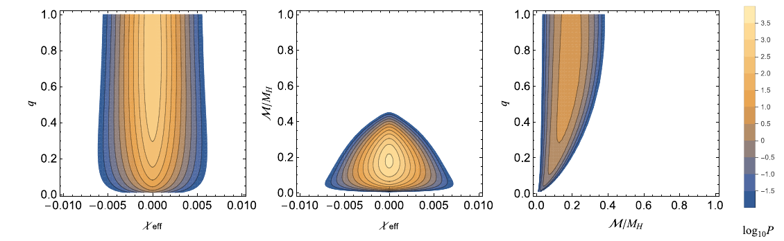
Figure 6: Contour map of the distribution functions of $(\chi_{\rm eff},q)$, $(\chi_{\rm eff},{\cal M})$ and $({\cal M},q)$, where $\chi_{\rm eff}$, ${\cal M}$ and $q$ are the effective spin parameter, the Chirp mass and the mass ratio of the binary PBHs, respectively. Taken from Ref. Koga et al. (2022).

Based on this analysis, Koga, Harada, Tada, Yokoyama and Yoo (2022) Koga et al. (2022) calculated the distribution of the effective spin parameter $\chi_{\rm eff}$ of binary black holes, which is a well determined observable of the spins obtained from gravitational wave forms from inspiralling binaries. Figure 6 shows the distribution functions of the parameters $a_{*}$ and $M$ of the single PBHs and of $\chi_{\rm eff}$, the Chirp mass ${\cal M}$ and the mass ratio $q$ of the binary PBHs, respectively. Although there is a tendency for larger spins with the smaller masses because of the critical phenomena, the probabilities for large values of the spin parameters are strongly suppressed. See Ref. Koga et al. (2022) for details.

In the above analyses, it was assumed that the power spectrum of curvature perturbation is sharp in the momentum space. Recently, it has been revealed that if this assumption is relaxed, the root mean square of $a_{*}$ can be slightly larger for some set of broad power spectra than the sharp one but should still be bounded by the value of the order of $10^{-3}$ Banerjee and Harada (in preparation).

4.2 Spins of primordial black holes formed with a soft equation of state

It is interesting to ask how much the results in Sec. 4.1 depend on the properties of the matter fields in the cosmological phase when the PBHs formed. In particular, it was shown that the PBH production is significantly enhanced in the QCD crossover, where the effective value of $w$ drops from $1/3$ to $\sim 0.23$ Escrivà et al. (2023); Musco et al. (2024). Saito, Harada, Koga and Yoo (2023) Saito et al. (2023) showed that for a soft EOS parameterised by $p=w\rho$, the root mean square of $a_{*}$ is a decreasing function of $w$ and can be well fitted by the power law $\propto w^{-0.49}$. However, since the dependence is weak for $w\simeq 0.2-1/3$, the initial spins are only modestly enhanced for the QCD crossover such as to $\sim 0.003$ from $\sim 0.002$ for radiation. It also suggests that $a_{*}$ can be very large if $w\ll 1$, although the analysis in Ref. Saito et al. (2023) is not well justified in the limit $w\to 0$, where the treatment for matter domination should apply.

4.3 Spins of primordial black holes formed in (early) matter domination

Since PBH formation will be enhanced in the (early) matter-dominated phase, it is very important to predict the spins of them. As we have seen before, nonspherical effects may become important. In fact, Harada, Yoo, Kohri and Nakao (2017) Harada et al. (2017) investigated the effects of angular momentum for PBH formation in this phase. Both the first-order and second-order effects can potentially play important roles. The first-order effect generates angular momentum through the nonsphericity of the region to collapse to a black hole, which is generally misaligned with a mode of linear perturbation. This is schematically illustrated in Fig. 7. The second-order does it through the coupling of two independent modes of linear perturbation, which is illustrated in Fig. 1 of Ref. Harada et al. (2017).

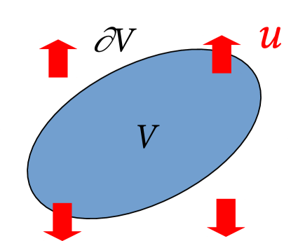
Figure 7: Schematic figures of the first-order effect to generate angular momentum. $V$ denotes the region that will collapse.

Although the dynamics of PBH formation in matter domination is expected to be very complicated, a perturbative calculation under certain working assumptions gives

$$\langle a_{*}^{2}\rangle\sim\sigma_{H}^{-1/2},$$ (21)

where $a_{*}$ is the nondimensional spin parameter of the region to collapse and $\sigma_{H}$ is the standard deviation of $\delta_{H}$ at the the horizon entry. Although the nondimensional numerical factor of the order of the unity on the right-hand side should be determined yet, this implies that most of PBHs have spins $a_{*}=O(1)$ if $\sigma_{H}\sim 0.1$. The angular momentum effects will strongly suppress PBH formation if $\sigma_{H}$ is even much smaller because of the Kerr bound $|a_{*}|\leq 1$. These results have recently been updated based on peak theory Saito et al. (in preparation).

4.4 Nonspherical simulation of PBH formation

Although we have so far discussed the initial spins of PBHs, we have neglected nonspherical nonlinear general relativistic dynamics in the formation of black holes for simplicity. It is clearly important to numerically simulate the nonspherical formation of PBHs and investigate how much the initially nonspherical initial data will affect the formation threshold and the initial spins of the produced PBHs. This is complementary to the perturbative analysis as it can check the validity of assumptions made.

Yoo, Harada and Okawa (2020) Yoo et al. (2020) implemented 3D numerical simulation of nonspherical PBH formation in radiation domination based on numerical relativity for the first time. They prepared the long-wavelength solutions as initial data, for which initial nonsphericity is expected to be typically very small according to peak theory. However, to make the numerical results clearer, they put $\sim 10\%$ nonsphericity in the initial data, which is much larger than the values expected from peak theory for PBH formation. They found that even such large nonsphericity changed the threshold of PBH formation only by $\sim 1\%$. See Figs 1 and 3 of Ref. Yoo et al. (2020) for the initial density perturbation on the left panel and the apparent horizon formation in the course of gravitational collapse on the right panel. We can see that in the simulation with the near-threshold value a very small apparent horizon forms at the very central region. This implies that we need very high resolution near the centre. This problem was attacked with a rescaled radial coordinate Yoo et al. (2020).

Yoo (2024) Yoo (2024) implemented further numerical relativity simulations for the EOS $p=w\rho$ with $w=0.2$ and $1/3$ with much higher resolution and accuracy. For this purpose, not only the rescaled radial coordinate but also the multi-level mesh refinement scheme were adopted. In such simulations, the estimation of the spin is not straightforward. In this work, it was implemented as follows. For the Kerr black hole, we can write the spin parameter $a_{*}$ using the event horizon configuration through the following relation

$$a_{*}=\frac{\sqrt{4\pi A(d^{2}-\pi A)}}{d^{2}},$$ (22)

where $d$ and $A$ are the equatorial circumference and the area, respectively. Yoo (2024) Yoo (2024) estimated the spin of the PBH as $|a_{*}|\ll 0.1$ assuming Eq. (22) for the numerically found apparent horizon. This is consistent with the perturbative estimates discussed in Secs. 4.1 and 4.2.

5 Type II perturbation and type B PBH

5.1 Positive curvature region, type II perturbation and separate universe condition

In the expanding universe, we assume that the decaying modes of perturbation can be neglected, while the growing modes will lead to structure formation including the formation of PBHs. The growing mode of perturbation with positive density perturbation will undergo the maximum expansion to form a self-gravitating object. Such regions can locally be well modelled by a positive-curvature FLRW spacetime surrounded by a flat FLRW spacetime Carr and Hawking (1974).

There are two independent physical length scales to characterise the spatial geometry, the curvature radius and the size of the curved region. This consideration implies the separate universe configuration if the latter becomes as large as possible Carr and Hawking (1974) as schematically illustrated in Fig. 8. It should be noted that this figure does not show the sequence of time evolution but each configuration gives a set of initial data for each time development of perturbation. It is physically interesting to think a nearly separate universe configuration, while a totally separate universe has nothing to do with our observable universe. Kopp, Hofmann and Weller (2010) Kopp et al. (2011) classified the configuration of the spatial geometry into type I and type II as shown in Fig. 8. The marginal case is given by a 3-hemisphere, while smaller and larger 3-spheres are called types I and II, respectively. The marginal configuration gives the possible maximum amplitude of the density perturbation Kopp et al. (2011); Carr and Harada (2015), despite the initial claim that the separate universe condition does Carr and Hawking (1974). Since the curvature perturbation is larger for type II than for type I, type II configurations are much rarer than type I in a standard probability distribution function of the curvature perturbation, whereas type II can be dominant in a particular inflationary scenario Escrivà et al. (2023).

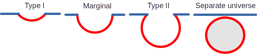
Figure 8: Classification of spatial configurations of overdense perturbations

5.2 Type II perturbation and its time development

Here we review the sets of initial data in terms of types I and II based on the recent work by Uehara, Escrivà, Harada, Saito and Yoo (2024) Uehara et al. (2024) for radiation domination. Here, the system is assumed to be spherically symmetric. They first constructed the long-wavelength solutions with choosing a function $\zeta(r)$. They chose the several choices for $\zeta$ but one of them is given by

$$\zeta(r)=\mu e^{-(1/2)k^{2}r^{2}}W(r),$$ (23)

where $W(r)$ is an appropriate window function and the constant $\mu$ gives the amplitude of perturbation. The areal radius $R$ and the Shibata-Sasaki compaction function ${\cal C}_{\rm SS}$ are plotted as functions of $r$ in Figs. 1(b) and 2(a) of Uehara et al. (2024), respectively, where we can see that for $\mu\gtrsim 1.4$, $R$ is no longer a monotonic function of the rescaled radial coordinate $z$, which implies that there is a throat and that ${\cal C}_{\rm SS}(r)$ has two peaks with the value $1/2$ and a minimum in between. See Ref. Uehara et al. (2024) for the account for this peculiar behaviour of the compaction function. These features are essentially the same in matter domination as discussed in Ref. Kopp et al. (2011) using the LTB solution.

Then, the time development of thus constructed initial data was constructed with a standard numerical relativity scheme based on the Baumgarte-Shapiro-Shibata-Nakamura formalism but adjusted for the spherical formation of PBHs. Figure 3 of Uehara et al. (2024) summarises the evolution of the spacetime for the long-wavelength solutions generated by the curvature perturbation given by Eq. (23). For $\mu=0.5$, the amplitude of perturbation is so small that it cannot collapse but disperse away. For $\mu=1.2$, the the amplitude of perturbation is so large that it can collapse to a black hole. The growth of the density contrast as well as the rapid decrease to zero of the lapse function $\alpha$ indicate the continued collapse to a black hole. This suggests that the critical value of $\mu$ for the black hole formation is between $0.5$ and $1.2$. For $\mu=1.8$, the time evolution of the density contrast and the lapse function does not look so different at least in qualitatively from that for $\mu=1.2$.

5.3 Type B horizon structure

To describe the horizons of the cosmological black holes, we introduce the trapped spheres and trapping horizons. See Refs. Hayward (1994, 1996) for the notion of trapped spheres and trapping horizons. For a spherically symmetric spacetime, we can generally introduce radial null coordinates $\xi_{\pm}$ such that the line element can be written in the following form:

$$ds^{2}=-2f(\xi_{+},\xi_{-})d\xi_{+}d\xi_{-}+R^{2}(\xi_{+},\xi_{-})(d\theta^{2}+\sin^{2}\theta d\phi^{2}).$$ (24)

We introduce the future-directed radial null vectors $l^{a}_{\pm}\propto(\partial_{\pm})^{a}$ such that $g_{ab}l^{a}_{+}l^{b}_{-}=-1$, where $\partial_{\pm}=\partial/\partial\xi_{\pm}$. Then, we call $\theta_{+}$ and $\theta_{-}$ outgoing and ingoing null expansions, respectively, where

$$\theta_{\pm}:=l^{a}_{\pm}\partial_{a}\ln(R^{2}).$$ (25)

We call a 2-sphere specified with $(\xi_{+},\xi_{-})$ a future (past) trapped sphere if $\theta_{+}\theta_{-}>0$ and $\theta_{+}+\theta_{-}<(>)0$. We call a 2-sphere specified with $(\xi_{+},\xi_{-})$ a future (past) marginal sphere if $\theta_{+}\theta_{-}=0$ and $\theta_{+}+\theta_{-}<(>)0$. We call a 2-sphere specified with $(\xi_{+},\xi_{-})$ a bifurcating marginal sphere if $\theta_{+}=\theta_{-}=0$. We call a 2-sphere specified with $(\xi_{+},\xi_{-})$ an untrapped sphere if $\theta_{+}\theta_{-}<0$. We call a spacetime region a future (past) trapped region, if any 2-sphere given by $(\xi_{+},\xi_{-})$ in the region is a future (past) trapped sphere. We call a spacetime region an untrapped region, if any 2-sphere given by $(\xi_{+},\xi_{-})$ in the region is an untrapped sphere. We call a hypersurface foliated by future (past) marginal spheres a future (past) trapping horizon. We call a hypersurface foliated by bifurcating marginal spheres a bifurcating trapping horizon Maeda et al. (2009).

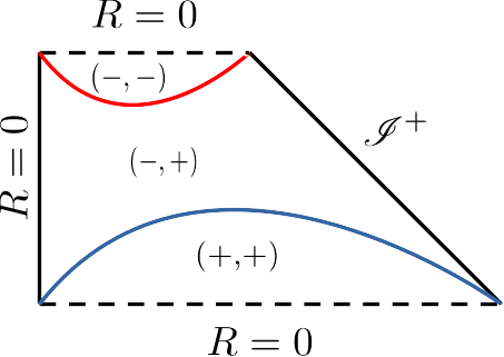
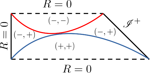
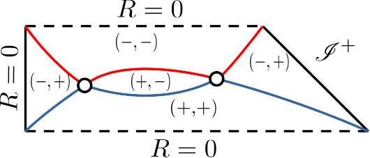
Figure 9: Structures of trapping horizons and trapped regions inferred by numerical simulations. The structures indicated on the top, middle and bottom panels are called type A, marginal and type B, respectively. The signs of the radial null expansions $({\rm sign}(\theta_{-}),{\rm sign}(\theta_{+}))$ are shown for each region. The regions are divided by trapping horizons, where $\theta_{+}\theta_{-}=0$. The future and past trapping horizons are denoted by the red and blue curves, respectively. The bifurcating trapping horizons are denoted by open circles. The black dashed lines denote spacetime singularities, while the black solid lines denote the regular centres and the null infinities. This figure is comparable to Fig. 7 of Ref. Uehara et al. (2024).

With the above terminology, we can now describe the structure of trapping horizons. We specify $\xi_{+}$ and $\xi_{-}$ as the null coordinates going to the outgoing and ingoing null coordinates in the far region which is asymptotic to the flat FLRW universe, which we assume to exist. There is a big difference in the structure of trapping horizons and trapped regions between $\mu=1.2$ and $\mu=1.8$. We schematically plot the horizon structures inferred by numerical simulations in Fig. 9. For $\mu=1.2$ as shown on the left panel, there are a past trapped region and a future-trapped region that are disconnected from each other with the associated past and future trapping horizons being separate. We call this horizon structure type A. For $\mu=1.8$ as shown on the right panel, it is very different. The past and future trapped regions have contacts at two points. The two points of intersection, which are in fact two 2-spheres, correspond to bifurcating trapping horizons. There appears an untrapped region in the centre enclosed by the future and past trapping horizons and the two bifurcating trapping horizons, where $\theta_{+}<0$ and $\theta_{-}>0$. We call this horizon structure type B.

This numerical result for the perturbation indicates that there appears the peculiar structure of trapping horizons and trapped regions, if $\mu$ is greater than some critical value. This was also true if we took another choice of $\zeta(r)$, so the above features are at least general to some extent. So, we can regard this structure as common for the sufficiently large amplitude of curvature perturbation of type II. We infer the existence of the marginal horizon structure between types A and B, which is shown on the middle panel of Fig, 9. So, we can say that a type II perturbation does not always result in a type B structure for radiation. This is due to the effect of pressure because it is known that for the dust case a type II perturbation necessarily entails the horizon structure of type B. So, we can conclude that there are at least PBHs with structure of types IA, IIA and IIB in radiation domination.

6 Summary

In the recent development of research on this subject, it has been revealed that PBHs lie at the intersection of various developing branches of modern physics.

In Sec. 2, we present the basic concept of PBHs. The mass of PBHs is usually considered to be on the mass scale within the cosmological horizon at the time of their formation. Mass accretion may significantly increase the PBH mass depending on the evolution scenario, whereas it has been shown to be negligible during the evolution in radiation domination. The mass of PBHs can be significantly reduced by Hawking evaporation, and they would have evaporated completely by now if they were lighter than the critical mass of approximately $10^{15}$ g, although the details of the evaporation process are still somewhat under debate. We obtain constraints on the fraction $f(M)$ of PBHs of mass $M$ in relation to all dark matter through different observations. The fraction $f(M)$ can be transformed into the formation probability $\beta(M)$ depending on the cosmological evolutionary scenario. The standard cosmic history implies that a very small value of $\beta(M)$, as small as $\sim 10^{-17}$ for $M\sim 10^{17}$ g, can yield $f(M)=O(1)$, i.e., can explain all dark matter, because the PBHs’ contribution to the energy of the Universe increases in proportion to the scale factor during the radiation-dominated phase.

In Sec. 3, we discuss PBH formation. A detailed and precise understanding of PBH formation physics has become increasingly important. The basic question in this study is how to predict $\beta(M)$ and other observationally significant quantities from a given cosmological scenario. Focusing on PBH formation from fluctuations generated by inflation, the key terms are inflation models, long-wavelength solutions, thresholds, softer EOS, matter domination, critical behaviours, and statistics.

In Sec 4, we discuss the initial spins of PBHs. PBHs formed during radiation domination are unlikely to have large spins. Perturbative studies show that the non-dimensional Kerr parameter of these PBHs is typically of the order of $10^{-3}$. In contrast, PBHs formed during matter domination can acquire large spins, at least initially. The effect of mass accretion after formation on the non-dimensional Kerr parameter needs to be studied carefully. It is evident that numerical simulations based on numerical relativity should shed light on this problem.

In Sec. 5, we review the recently implemented numerical relativity simulations of the time evolution of type II perturbations during radiation domination. This is particularly relevant to a very rare perturbation peak or to a specific inflationary scenario. The resulting structures of trapping horizons can be classified into two types: one is standard for PBHs, and the other is very unique, featuring the crossing of trapping horizons as bifurcating trapping horizons. We refer to these as types A and B, respectively, while we can also discuss the marginal structure. The numerical simulations suggest that the evolution of type II perturbations can be classified into type A and type B based on their horizon structure. Thus, we may call them types IIA and IIB.

Finally, the author must acknowledge that there are many interesting issues concerning the formation of PBHs that cannot even be mentioned in this article. The study of PBH formation not only requires a deep understanding of physical phenomena within known standard physics but also offers the opportunity to explore unknown new physics through PBHs. Both of these aspects will play important roles in the future of PBH formation studies.