Bayesian CART models for aggregate claim modeling

Abstract

This paper proposes three types of Bayesian CART (or BCART) models for aggregate claim amount, namely, frequency-severity models, sequential models and joint models. We propose a general framework for the BCART models applicable to data with multivariate responses, which is particularly useful for the joint BCART models with a bivariate response: the number of claims and aggregate claim amount. To facilitate frequency-severity modeling, we investigate BCART models for the right-skewed and heavy-tailed claim severity data by using various distributions. We discover that the Weibull distribution is superior to gamma and lognormal distributions, due to its ability to capture different tail characteristics in tree models. Additionally, we find that sequential BCART models and joint BCART models, which incorporate dependence between the number of claims and average severity, are beneficial and thus preferable to the frequency-severity BCART models in which independence is assumed. The effectiveness of these models’ performance is illustrated by carefully designed simulations and real insurance data.

Keywords: average severity; dependence; DIC; information sharing; zero-inflated compound Poisson gamma distribution.

1 Introduction

In the classical formula of non-life insurance pricing, the pure premium is determined by multiplying the expected claim frequency with the conditional expectation of average severity, assuming independence between the number of claims and claim amounts; see, e.g., [1, 2] and references therein. With the assumed independence, the frequency-severity models treat these two components separately by generalized linear models (GLMs) traditionally, assuming distributions from the exponential family. The frequency study focuses on the occurrences of claims, and the severity study — provided that a claim has occurred — investigates the claim amount. In recent years, a growing body of literature emphasizes the importance of understanding the interrelated nature of claim occurrences and their associated claim amounts to improve model applicability.

There are two widely discussed strategies to address the issue of dependence. The first one, known as the copula method, is commonly employed to model the dependence structure between the number of claims and claim amounts; see, e.g., [3, 4, 5] and references therein. By the nature of the number of claims and claim amounts, the dependence modeling requires the development of mixed copula for which some margins are discrete and others are continuous. We refer to [6, 7] for relevant discussions. In parallel, the adoption of Bayesian approaches to copula modeling, as seen in [8], has contributed to refining copula-based modeling techniques. By augmenting the likelihood with latent variables and employing efficient Markov Chain Monte Carlo (MCMC) sampling schemes, copula models with discrete margins can be estimated using the resulting augmented posterior; see, e.g., [9]. However, the challenge persists in selecting the appropriate copula family and parameters, as discussed in [10, 11, 12]. A second strategy is to directly enable the severity component of the model to depend on the frequency component. Specifically, the number of claims is introduced as a covariate in the average severity modeling, formulating a conditional severity model; see, e.g., [13, 14]. This method has been popular because it is easy to implement and interpret.

As a comparable alternative, the aggregate claim cost can be directly modeled using Tweedie’s model which assumes a Poisson sum of gamma variables for the aggregate claim amount. This modeling approach simplifies the analysis by accommodating discrete claim numbers and continuous claim amounts in one distribution; see, e.g., [15]. Concurrently, discussions regarding the suitability of GLMs for aggregate claim amount analysis have focused on the trade-off between model complexity and predictive performance, emphasizing the benefits and contexts where Tweedie’s model excels and where alternative methodologies may be better; see, e.g., [16]. Recently, a novel approach is introduced to reduce computational costs for Tweedie’s parameter estimation within GLMs, as seen in [17]. In a related advance, [18] proposed fitting the Tweedie distribution within GLMs through the Expectation-Maximization (EM) algorithm, which is conceptually analogous to iteratively re-weighted Poisson-gamma modeling on an augmented dataset. This approach simplifies the problem by leveraging expectations of latent variables. Numerical examples indicate that the EM-based method outperforms the traditional likelihood maximization approach, particularly in terms of computational efficiency and accuracy. We refer to [19, 18, 20] for recent developments of Tweedie’s model. While both are considered in the literature, the insurance industry typically favours the separated frequency-severity models.

More recently, machine learning methods have been introduced in the context of insurance by adopting actuarial loss distributions to capture the characteristics of insurance claims. We refer to [21, 22, 1, 23, 24] for recent discussions. Insurance pricing models are heavily regulated and must meet specific requirements before being deployed in practice, which poses challenges for most machine learning methods. As discussed in [2, 24], tree models are considered appropriate for insurance rate-making due to their transparent nature. In our previous work [24], we have demonstrated the superiority of Bayesian classification and regression tree (BCART) models in claim frequency analysis. In this sequel we construct some novel insurance pricing models using BCART for both average severity and aggregate claim amount.

Specifically, inspired by the types of claim loss models discussed above, we introduce and investigate three corresponding types of BCART models. We first discuss a benchmark frequency-severity BCART model, where the number of claims and average severity are modeled separately using BCART. Furthermore, We propose two other types of BCART models, with an aim to incorporate the underlying dependence between the number of claims and average severity. These are sequential BCART models (motivated by [13, 14]) and joint BCART models (motivated by [15, 25]). In contrast to the frequency-severity and sequential BCART models which result in two separate trees for the number of claims and average severity, the joint BCART models generate one joint tree for the aggregate claim amount.

The main contributions of this paper are as follows:

• We implement BCART models for average severity including gamma, lognormal and Weibull distributions and for aggregate claim amount including compound Poisson gamma (CPG) and zero-inflated compound Poisson gamma (ZICPG) distributions. These are not currently available in any R package.

• To explore the potential dependence between the number of claims and average severity, we propose novel sequential BCART models that treat the number of claims (or its estimate) as a covariate in average severity modeling. The effectiveness is illustrated using simulated and real insurance data.

• We present a general framework for the BCART models applicable for multivariate responses, extending the MCMC algorithms discussed in [24]. There have been very few discussions on Bayesian tree models with multivariate responses in the current literature, with the only exception [26] as we are aware of. As a particular application, we propose novel joint BCART models with a bivariate response to simultaneously model the number of claims and aggregate claim amount. In doing so, we employ the commonly used distributions such as CPG and ZICPG. The potential advantages of information sharing using one joint tree compared with two separate trees are also illustrated by simulated and real insurance data.

• For the comparison of one joint tree (generated from the joint BCART models) with two separate trees (generated from the frequency-severity or sequential BCART models), we propose some evaluation metrics which involve a combination of trees using an idea of [27]. We also propose an application of the Adjusted Rand Index (ARI) in assessing the similarity between trees. Although ARI is widely used in cluster analysis, its application to tree comparisons seems to be a novel idea. The use of ARI enhances the understanding of the necessity of information sharing, an aspect not covered in relevant literature; see, e.g., [28].

Outline of the rest of the paper: In Section 2, we briefly review the BCART framework, introducing a more general MCMC algorithm for BCART models with multivariate responses. Section 3 introduces the notation for insurance claim data and investigates three types of BCART models for the aggregate claim amount. Section 4 develops a performance assessment of the proposed aggregate claim models using simulation examples. In Section 5, we present a detailed analysis of real insurance data using the proposed models. Section 6 concludes the paper.

2 Bayesian CART: A general framework

The BCART models, as introduced in the seminal papers [29, 30], provide a Bayesian perspective on CART models. In this section, we give a brief review of the BCART model using a more general framework that applies to multivariate response data; see [24] for the univariate case.

2.1 Data, model and training algorithm

Consider a matrix-form dataset $(\bm{X},\bm{Y})=\big{(}(\bm{x}_{1},\bm{y}_{1}),(\bm{x}_{2},\bm{y}_{2}),\ldots,(\bm{x}_{n},\bm{y}_{n})\big{)}^{\top}$ with $n$ indepedent observations. For the $i$-th observation, $\bm{x}_{i}=(x_{i1},x_{i2},\ldots,x_{ip})$ is a vector of $p$ explanatory variables (or covariates) sampled from a space $\mathcal{X}$, while $\bm{y}_{i}=(y_{i1},y_{i2},\ldots,y_{iq})$ is a vector of $q$ response variables sampled from a space $\mathcal{Y}$. For the severity (or frequency) modeling, $\mathcal{Y}$ is a space of real positive (or integer) values. For aggregate claim modeling, $\mathcal{Y}$ is a space of 2-dimensional vectors with two components: an integer number of claims and a real valued aggregate claim amount.

A CART has two main components: a binary tree $\mathcal{T}$ with $b$ terminal nodes which induces a partition of the covariate space $\mathcal{X}$, denoted by $\left\{\mathcal{A}_{1},\ldots,\mathcal{A}_{b}\right\}$, and a parameter $\bm{\theta}=\left(\bm{\theta}_{1},\bm{\theta}_{2},\ldots,\bm{\theta}_{b}\right)$ which associates the parameter value $\bm{\theta}_{t}$ with the $t$-th terminal node. Note that here we do not specify the dimension and range of the parameter $\bm{\theta}_{t}$ which should be clear from the context. If $\bm{x_{i}}$ is located in the $t$-th terminal node (i.e., $\bm{x}_{i}\in\mathcal{A}_{t}$), then $\bm{y}_{i}$ has a (joint) distribution $f\left(\bm{y}_{i}\mid\bm{\theta}_{t}\right)$, where $f$ represents a parametric family indexed by $\bm{\theta}_{t}$. By associating observations with the $b$ terminal nodes in the tree $\mathcal{T}$, we can re-order the $n$ observations such that

$$(\bm{X},\bm{Y})=\big{(}(\bm{X}_{1},\bm{Y}_{1}),(\bm{X}_{2},\bm{Y}_{2})\ldots,(\bm{X}_{b},\bm{Y}_{b})\big{)}^{\top},$$

where $\bm{Y}_{t}=\left(\bm{y}_{t1},\ldots\bm{y}_{tn_{t}}\right)^{\top}$ is an $n_{t}\times q$ matrix with $n_{t}$ denoting the number of observations and $\bm{y}_{ti}$ denoting the $i$-th observed response in the $t$-th terminal node, and $\bm{X}_{t}$ is an analogously defined $n_{t}\times p$ design matrix. We make the typical assumption that conditionally on $(\bm{\theta},\mathcal{T})$, response variables are independent and identically distributed (IID). The CART model likelihood is then

$$p(\bm{Y}\mid\bm{X},\bm{\theta},\mathcal{T})=\prod_{t=1}^{b}f\left(\bm{\bm{Y}}_{t}\mid\bm{\theta}_{t}\right)=\prod_{t=1}^{b}\prod_{i=1}^{n_{t}}f\left(\bm{y}_{ti}\mid\bm{\theta}_{t}\right).$$ (1)

Given $(\bm{\theta},\mathcal{T})$, a Bayesian analysis involves specifying a prior distribution $p(\bm{\theta},\mathcal{T})$, and inference about $\bm{\theta}$ and $\mathcal{T}$ is based on the joint posterior $p(\bm{\theta},\mathcal{T}|\bm{Y},{\color[rgb]{0,0,0}\bm{X}})$ using a suitable MCMC algorithm. Since $\bm{\theta}$ indexes the parametric model whose dimension depends on the number of terminal nodes of the tree, it is usually convenient to apply the relationship $p(\bm{\theta},\mathcal{T})=p(\bm{\theta}\mid\mathcal{T})p(\mathcal{T})$, and specify the tree prior distribution $p(\mathcal{T})$ and the terminal node parameter prior distribution $p(\bm{\theta}\mid\mathcal{T})$, respectively. This strategy, introduced by [31], offers several advantages for Bayesian model selection as outlined in [29].

The prior distribution $p(\mathcal{T})$ has two components: a tree topology and a decision rule for each of the internal nodes. We follow [29], in which a draw of the tree is obtained by generating, for each node at depth $d$ (with $d=0$ for the root node), two child nodes with probability

$$p(d)=\gamma\left(1+d\right)^{-\rho},$$ (2)

where $\gamma{\color[rgb]{0,0,0}\in(0,1]},\rho\geq 0$ are parameters controlling the structure and size of the tree. This process iterates for $d=0,1,\ldots,$ until we reach a depth at which all the nodes cease growing. After the tree topology is generated, each internal node is associated with a decision rule which will be drawn uniformly among all the possible decision rules for that node. We refer to [24] for detailed discussion on the choice of the prior distribution $p(\mathcal{T})$.

It is important to choose the form $p(\bm{\theta}\mid\mathcal{T})$ for which it is possible to analytically margin out $\bm{\theta}$ to obtain the integrated likelihood

$$p(\bm{Y}\mid\bm{X},\mathcal{T}) =\int p(\bm{Y}\mid\bm{X},\bm{\theta},\mathcal{T})p(\bm{\theta}\mid\mathcal{T})d{\bm{\theta}}=\prod_{t=1}^{b}\int f\left(\bm{Y}_{t}\mid\bm{\theta}_{t}\right)p(\bm{\theta}_{t})d\bm{\theta}_{t}$$

$$=\prod_{t=1}^{b}\int\prod_{i=1}^{n_{t}}f\left(\bm{y}_{ti}\mid\bm{\theta}_{t}\right)p(\bm{\theta}_{t})d\bm{\theta}_{t},$$ (3)

where in the second equality we assume that conditional on the tree $\mathcal{T}$ with $b$ terminal nodes as above, the parameters $\bm{\theta}_{t},t=1,2,\ldots,b$, have IID priors $p(\bm{\theta}_{t})$, which is a common assumption. Examples where this integration has a closed-form expression can be found in, e.g., [29, 32].

When there is no obvious prior distribution $p(\bm{\theta}_{t})$ such that the integration in (2.1) is of closed-form, particularly, for non-Gaussian distributed data $\bm{Y}$, a data augmentation method is usually utilized in the literature, e.g., [33, 24]. Here, we present a general framework in which apart from including a data augmentation, some components of $\bm{\theta}_{t}$ are assumed to be known a priori, but some others are assumed to be unknown. More precisely, we assume $\bm{\theta}_{t}=(\bm{\theta}_{t,M},\bm{\theta}_{t,B})$, where $\bm{\theta}_{t,M}$ are the parameters that are treated as known and computed using Method of Moments Estimation (MME), or Maximum Likelihood Estimation (MLE), and $\bm{\theta}_{t,B}$ are the unknown parameters that need to be estimated in the Bayesian framework. This newly proposed framework aims to reduce the overall computational time of the algorithm and overcome the difficulty of finding an appropriate prior for some parameters even with the data augmentation (that is why $\bm{\theta}_{t,M}$ is assumed known a priori). Under this framework, we augment the data $\bm{Y}$ by introducing a latent variable $\bm{Z}=(\bm{z}_{1},\bm{z}_{2},\ldots,\bm{z}_{n})^{{\color[rgb]{0,0,0}\top}}$ so that the integration in (4) is computable for augmented data $(\bm{Y},\bm{Z})$. The integrated likelihood is given as

$$p(\bm{Y}\mid\bm{X},{\color[rgb]{0,0,0}\bm{\theta}_{M},}\mathcal{T})=\int p(\bm{Y},\bm{Z}\mid\bm{X},{\color[rgb]{0,0,0}\bm{\theta}_{M},}\mathcal{T})d\bm{Z},$$

where

$$p(\bm{Y},\bm{Z}\mid\bm{X},{\color[rgb]{0,0,0}\bm{\theta}_{M},}\mathcal{T}) =\int p(\bm{Y},\bm{Z}\mid\bm{X},\bm{\theta}_{M},\bm{\theta}_{B},\mathcal{T})p(\bm{\theta}_{B}\mid\mathcal{T})d{\bm{\theta}_{B}}$$ (4)

$$=\prod_{t=1}^{b}\int\prod_{i=1}^{n_{t}}f\left(\bm{y}_{ti},\bm{z}_{ti}\mid\bm{\theta}_{t,M},\bm{\theta}_{t,B}\right)p(\bm{\theta}_{t,B})d\bm{\theta}_{t,B},$$

with $\bm{Z}_{t}=(\bm{z}_{t1},\bm{z}_{t2},\ldots,\bm{z}_{tn_{t}})^{{\color[rgb]{0,0,0}\top}}$ defined according to the partition of $\mathcal{X}$.

Combining the augmented integrated likelihood $p(\bm{Y},\bm{Z}\mid\bm{X},{\color[rgb]{0,0,0}\bm{\theta}_{M},}\mathcal{T})$ with tree prior $p(\mathcal{T})$, allows us to calculate the posterior of $\mathcal{T}$

$$p(\mathcal{T}\mid\bm{X},\bm{Y},{\color[rgb]{0,0,0}\bm{\theta}_{M},}\bm{Z})\propto p(\bm{Y},\bm{Z}\mid\bm{X},{\color[rgb]{0,0,0}\bm{\theta}_{M},}\mathcal{T})p(\mathcal{T}).$$ (5)

When using MCMC to conduct Bayesian inference, $\mathcal{T}$ can be updated using a Metropolis-Hastings (MH) algorithm with the right-hand side of (5) used to compute the acceptance ratio. Starting from the root node, the MCMC algorithm for simulating a Markov chain sequence of pairs $(\bm{\theta}^{(1)},\mathcal{T}^{(1)}),(\bm{\theta}^{(2)},\mathcal{T}^{(2)}),\ldots,$ using the posterior given in (5), is given in Algorithm 1 in which commonly used proposals (or transitions) for $q(\cdot,\cdot)$ include grow, prune, change and swap (see [29]). See [24] for further details.

Algorithm 1 One step of the MCMC algorithm for the BCART models parameterized by $(\bm{\theta}_{M},\bm{\theta}_{B},\mathcal{T})$ using data augmentation with both known and unknown parameters

Input: Data $(\bm{X},\bm{Y})$ and current values $(\hat{\bm{\theta}}_{M}^{(m)},\bm{\theta}_{B}^{(m)},\bm{Z}^{(m)},\mathcal{T}^{(m)})$
       1: Generate a candidate value $\mathcal{T}^{*}$ with probability distribution $q(\mathcal{T}^{(m)},\mathcal{T}^{*})$
       2: Estimate $\hat{\bm{\theta}}_{M}^{(m+1)}$, using MME (or MLE)
       3: Sample $\bm{Z}^{(m+1)}\sim p(\bm{Z}\mid\bm{X},\bm{Y},\hat{\bm{\theta}}_{M}^{(m+1)},\bm{\theta}_{B}^{(m)},\mathcal{T}^{(m)})$
       4: Set the acceptance ratio

$$\alpha(\mathcal{T}^{(m)},\mathcal{T}^{*})=\min\left\{\frac{q(\mathcal{T}^{*},\mathcal{T}^{(m)})p(\bm{Y},\bm{Z}^{(m+1)}\mid\bm{X},\hat{\bm{\theta}}_{M}^{(m+1)},\mathcal{T}^{*})p(\mathcal{T}^{*})}{q(\mathcal{T}^{(m)},\mathcal{T}^{*})p(\bm{Y},\bm{Z}^{(m)}\mid\bm{X},\hat{\bm{\theta}}_{M}^{(m)},\mathcal{T}^{(m)})p(\mathcal{T}^{(m)})},1\right\}$$

5: Update $\mathcal{T}^{(m+1)}=\mathcal{T}^{*}$ with probability $\alpha(\mathcal{T}^{(m)},\mathcal{T}^{*})$, otherwise, set $\mathcal{T}^{(m+1)}=\mathcal{T}^{(m)}$
       6: Sample $\bm{\theta}_{B}^{(m+1)}\sim p(\bm{\theta}_{B}\mid\bm{X},\bm{Y},\hat{\bm{\theta}}_{M}^{(m+1)},\bm{Z}^{(m+1)},\mathcal{T}^{(m+1)})$
  Output: New values $(\hat{\bm{\theta}}_{M}^{(m+1)},\bm{\theta}_{B}^{(m+1)},\bm{Z}^{(m+1)},\mathcal{T}^{(m+1)})$

Remark 1

(a). In Algorithm 1, the sampling steps should be done only as required. For example, in Step 2, $\hat{\bm{\theta}}_{M}^{(m+1)}$ needs to be estimated only for those nodes that were involved in the proposed move from $\mathcal{T}^{(m)}$ to $\mathcal{T}^{*}$.

(b). Algorithm 1 is a general algorithm from which we can retrieve all the algorithms discussed in [24], e.g., the algorithm for the zero-inflated Poisson model therein can be retrieved by assuming there is no component $\bm{\theta}_{M}$.

2.2 Model selection and prediction

The MCMC algorithm described in Algorithm 1 can be used to search for desirable trees, and we use the three-step approach proposed in [24] to select an “optimal” tree among those visited trees; see Table 1. To this end, we let $m_{s}<m_{e}$ be two user input integers which represent the belief of where the optimal number of terminal nodes of the tree might fall into. Note that in the following sections, we introduce the DIC for different models based on the idea that DIC$=$“goodness of fit”$+$“complexity”. See [34, 35] for discussion on DIC in a general Bayesian framework.

Table 1: Three-step approach for “optimal” tree selection

Step 1:	Set a sequence of hyper-parameters $(\gamma_{j},\rho_{j}),j=m_{s},\cdots,m_{e},$ such that for $(\gamma_{j},\rho_{j})$, the MCMC algorithm converges to a region of trees with $j$ terminal nodes.
Step 2:	For each $j$ in Step 1, select the tree with maximum likelihood $p(\bm{Y}\mid\bm{X},\bm{\overline{\bm{\theta}}},\mathcal{T})$ from the convergence region, where $\bm{\overline{\bm{\theta}}}$ is an output from Algorithm 1.
Step 3:	From the trees obtained in Step 2, select the optimal one using deviance information criterion (DIC).

Suppose $\mathcal{T}$, with $b$ terminal nodes and parameter $\overline{\bm{\theta}}$, is the selected tree from the above approach. For new $\bm{x}$ the predicted $\hat{\bm{y}}$ is defined as

$$\hat{\bm{y}}\mid\bm{x}=\sum_{t=1}^{b}E(\bm{y}\mid\bar{\bm{\theta}}_{t})I_{(\bm{x}\in\mathcal{A}_{t})},$$ (6)

where $I_{(\cdot)}$ denotes the indicator function and $\{\mathcal{A}_{t}\}_{t=1}^{b}$ is the partition of $\mathcal{X}$ by $\mathcal{T}$.

3 Aggregate claim amount modeling with Bayesian CART

This section introduces the BCART models for aggregate claim amount by specifying the response distribution within the framework outlined in Section 2. We begin by introducing the type of insurance claim data that will be discussed in this paper. A claim dataset with $n$ policyholders can be described by $(\bm{X},\bm{v},\bm{N},\bm{S})=\big{(}(\bm{x}_{1},v_{1},N_{1},S_{1}),\ldots,(\bm{x}_{n},v_{n},N_{n},S_{n})\big{)}^{\top}$, where $\bm{x}_{i}=(x_{i1},\ldots,x_{ip})\in\mathcal{X}$ represents rating variables (e.g., driver age, age of the car and car brand in car insurance); $v_{i}\in(0,1]$ is the exposure in yearly units, quantifying the duration the policyholder $i$ is exposed to risk; $N_{i}$ is the number of claims reported during exposure time of the policyholder, and $S_{i}$ is the aggregate (total) claim amount.

Before describing our models, we recall some basics on the aggregate claim amount modeling as motivation; see, e.g., [36, 14, 3] for discussions. Consider a given (generic) policyholder, and assume unit exposure (i.e., $v=1$), for simplicity. The aggregate claim amount of the policyholder can be expressed as

$$S=\sum_{j=1}^{N}Y_{j},$$ (7)

where $N$ is the number of claims within a year and $Y_{j}$ denotes the severity of the $j$-th claim. It is also assumed that $Y_{1},Y_{2},...,Y_{N}$, given $N$, are IID positive random variables which are independent of $N$. Let $Y$ denote a generic random variable for claim severity and, by convention, $S=0$ when $N=0$.

We are primarily interested in estimating the pure premium defined as $\mathbb{E}(S)$ (we remark that generally the pure premium should be defined as $\mathbb{E}(S)/v$, i.e., the expected claim amount per year). We also define the average severity as $\bar{S}=S/N$ when $N>0$ and $\bar{S}=0$ when $N=0$. It can be easily derived that

$$\mathbb{E}(S)=\mathbb{E}(N)\mathbb{E}(Y)=\mathbb{E}(N)\mathbb{E}(\bar{S}|N>0).$$ (8)

When a vector $\bm{x}=(x_{1},\ldots,x_{p})$ of covariates for this policyholder is available, it can be incorporated into a pricing model through separate models for frequency $\mathbb{E}(N)$ and severity $\mathbb{E}(Y)$ (or average severity $\mathbb{E}(\bar{S}|N>0)$), this is the so-called frequency-severity model. Traditionally, both frequency and (average) severity components are modeled by GLMs. In the literature (see, e.g., [2, 37, 38]), there are two ways to model the average severity; one is to model claim severity $Y_{j}(j=1,2,\ldots,N)$ which induces a model for the average severity $\bar{S}$, and the other way is to directly model the average severity $\bar{S}$ when $N>0$. In the first way, the distribution for $Y_{j}$ is usually restricted to the exponential distribution family (EDF) due to the convolution property. More precisely, assuming $Y_{j}\sim\text{EDF}(\mu,\phi)$, with mean $\mu$ and dispersion $\phi$, we have, $\bar{S}|N>0\sim\text{EDF}(\mu,\phi/N)$, which means that modeling severity is equivalent to modeling the average severity only when $N$ is included as a weight in the model for $\bar{S}.$ In the second way, $\bar{S}|N>0$ is directly modeled, the choice of its distribution is thus much richer. These are discussed in Section 3.1.

Next, we discuss the covariance between $S$ (or $\bar{S}$) and $N$. We have

$$\text{Cov}(S,N)=\mathbb{E}(SN)-\mathbb{E}(S)\mathbb{E}(N)=\mathbb{E}(Y)\text{Var}(N)>0,$$

$$\text{Cov}(S,N|N>0)=\mathbb{E}(SN|N>0)-\mathbb{E}(S|N>0)\mathbb{E}(N|N>0)=\frac{\mathbb{E}(Y)\text{Var}(N)}{1-\mathbb{P}(N=0)}>0,$$

which means that $S$ and $N$ (or given $N>0$) are obviously correlated. Furthermore,

$$\text{Cov}(\bar{S},N)=\mathbb{E}(S)-\mathbb{E}(\bar{S})\mathbb{E}(N)=\mathbb{P}(N=0)\mathbb{E}(Y)\text{Var}(N)>0,$$

$$\text{Cov}(\bar{S},N|N>0)=\mathbb{E}(S|N>0)-\mathbb{E}(\bar{S}|N>0)\mathbb{E}(N|N>0)=0,$$

which means that $\bar{S}$ and $N$ are also correlated, but $\bar{S}$ and $N$ given $N>0$ are uncorrelated. However, $\bar{S}$ and $N$ given $N>0$ are not generally independent; see [3] for a simple argument.

The above calculations show that model (7) is plausible for data with positive or zero correlations between the number of claims and severity. However, as discussed in [14], the number of claims and average severity are often negatively correlated in many types of insurance data, particularly, in collision automobile insurance data. In our real data analysis below, we observe a similar negative correlation, following the approach in [14]. To better model this type of data and capture the underlying dependence between the number of claims and average severity, we introduce two other types of BCART models. First, following the idea of [13, 14] we introduce the sequential BCART models by including $N$ (or its estimate $\hat{N}$) as a covariate when modeling the average severity in (8). Second, motivated by [15, 25], we introduce joint BCART models by considering $(N,S)$ as a bivariate response. By its nature, the dependence between the number of claims and average severity is directly incorporated in the sequential BCART models. In the joint BCART models, the dependence caused by potentially shared information (through covariates) can be captured in a selected single tree. These BCART models will be discussed in detail in Sections 3.2 and 3.3, respectively.

3.1 Frequency-severity BCART models

Recall that the BCART models for the frequency component $\mathbb{E}(N)$ of (8) have been discussed in [24]. Here we shall focus on the BCART modeling of the average severity component $\mathbb{E}(\bar{S}|N>0)$ of (8). More precisely, we will discuss a gamma distribution (as an example in the EDF) with $N$ included as a weight, and three other distributions to directly model the average severity without including $N$ as a weight, namely, gamma, lognormal, and Weibull. For this purpose, we will only consider a data subset with $N_{i}>0$, and denote by $\bar{n}$ $(\leq n)$ the size of this subset. The subset of average severity data will be denoted by $(\bm{X},\bm{N},\bm{\bar{S}})=\big{(}(\bm{x}_{1},N_{1},\bar{S}_{1}),\ldots,(\bm{x}_{\bar{n}},N_{\bar{n}},\bar{S}_{\bar{n}})\big{)}^{\top}$.

3.1.1 Average severity modeling using gamma distribution with $N$ as a weight

Assume the generic average severity $\bar{S}|N>0$ follows a gamma distribution with parameters being multipliers of $N$, i.e., $\bar{S}|N>0\sim\text{Gamma}\ (N\alpha,N\beta),$ with $\alpha,\beta>0$. Note that this is equivalent to assuming that the individual severity $Y_{j}$ follows Gamma($\alpha,\beta$) distribution, due to the convolution property. Recall that the probability density function (pdf) of the Gamma($\alpha,\beta$) distribution and its mean and variance are given as

$$f_{G}(x)=\frac{\beta^{\alpha}x^{\alpha-1}}{\Gamma(\alpha)}e^{-\beta x},\ x>0,\ \ \ \ \mu_{G}=\frac{\alpha}{\beta},\ \ \sigma_{G}^{2}=\frac{\alpha}{\beta^{2}},$$ (9)

where $\Gamma(\cdot)$ is the gamma function. It is known that gamma distribution is right-skewed and relatively light-tailed.

According to the general BCART framework in Section 2, considering a tree $\mathcal{T}$ with $b$ terminal nodes and $\bm{\theta}_{t}=(\alpha_{t},\beta_{t})$ the two-dimensional parameter for the $t$-th terminal node, we assume $\bar{S}_{i}|\bm{x}_{i},N_{i}\sim\text{Gamma}\ \left(N_{i}\alpha(\bm{x}_{i}),N_{i}\beta(\bm{x}_{i})\right)$ for the $i$-th observation, where $\alpha(\bm{x}_{i})=\sum_{t=1}^{{\color[rgb]{0,0,0}b}}\alpha_{t}I_{(\bm{x}_{i}\in\mathcal{A}_{t})}$ and $\beta(\bm{x}_{i})=\sum_{t=1}^{b}\beta_{t}I_{(\bm{x}_{i}\in\mathcal{A}_{t})}$, with $\{\mathcal{A}_{t}\}_{t=1}^{b}$ being the corresponding partition of $\mathcal{X}$. Specifically, for $i$-th observation such that $\bm{x}_{i}\in\mathcal{A}_{t}$, we have (with $N_{i}$ compressed in $f_{G}$)

$$f_{\text{G}}\left(\bar{S}_{i}|\alpha_{t},\beta_{t}\right)=\frac{(N_{i}\beta_{t})^{N_{i}\alpha_{t}}\bar{S}_{i}^{N_{i}\alpha_{t}-1}}{\Gamma(N_{i}\alpha_{t})}e^{-N_{i}\beta_{t}\bar{S}_{i}}.$$

The mean and variance of $\bar{S}_{i}$ are thus given by $\alpha_{t}/\beta_{t}$ and $\alpha_{t}/(N_{i}\beta_{t}^{2})$, respectively.

For each terminal node $t$, we treat $\alpha_{t}$ as known and $\beta_{t}$ as unknown and shall not apply any data augmentation. According to the notation used in Section 2 this means $\bm{\theta}_{t,M}=\alpha_{t}$ and $\bm{\theta}_{t,B}=\beta_{t}$. Here $\alpha_{t}$ will be estimated using MME, i.e.,

$$\hat{\alpha}_{t}=\frac{(\bar{S})_{t}^{2}}{\text{Var}(\bar{S})_{t}\bar{N}_{t}},$$ (10)

where $(\bar{S})_{t}$ and $\text{Var}(\bar{S})_{t}$ are the empirical mean and variance of the average severity, respectively, and $\bar{N}_{t}$ is the average claim number of the data in the $t$-th terminal node. We treat $\beta_{t}$ as uncertain and use a conjugate gamma prior with hyper-parameters $\alpha_{\pi},\beta_{\pi}>0$. Denote the associated data in terminal node $t$ as $\left(\bm{X}_{t},\bm{N}_{t},\bm{\bar{S}}_{t})=(({X}_{t1},N_{t1},\bar{S}_{t1}),\ldots,({X}_{t\bar{n}_{t}},N_{t\bar{n}_{t}},\bar{S}_{t\bar{n}_{t}})\right)^{\top}$. The integrated likelihood for the terminal node $t$ can then be obtained as

$$p_{\text{G}}(\bm{\bar{S}}_{t}\mid\bm{X}_{t},\bm{N}_{t},\hat{\alpha}_{t}) =\int_{0}^{\infty}f_{\text{G}}(\bm{\bar{S}}_{t}\mid\bm{N}_{t},\hat{\alpha}_{t},\beta_{t})p(\beta_{t})d\beta_{t}$$

$$=\int_{0}^{\infty}\prod_{i=1}^{\bar{n}_{t}}\left(\frac{(N_{ti}\beta_{t})^{N_{ti}\hat{\alpha}_{t}}\bar{S}_{ti}^{N_{ti}\hat{\alpha}_{t}-1}e^{-N_{ti}\beta_{t}\bar{S}_{ti}}}{\Gamma(N_{ti}\hat{\alpha}_{t})}\right)\frac{\beta_{\pi}^{\alpha_{\pi}}{\beta_{t}}^{\alpha_{\pi}-1}e^{-\beta_{\pi}\beta_{t}}}{\Gamma(\alpha_{\pi})}d\beta_{t}$$ (11)

$$=\frac{\beta_{\pi}^{\alpha_{\pi}}\prod_{i=1}^{\bar{n}_{t}}\left(N_{ti}^{N_{ti}\hat{\alpha}_{t}}\bar{S}_{ti}^{N_{ti}\hat{\alpha}_{t}-1}\right)}{\Gamma(\alpha_{\pi})\prod_{i=1}^{\bar{n}_{t}}\Gamma(N_{ti}\hat{\alpha}_{t})}\frac{\Gamma(\sum_{i=1}^{\bar{n}_{t}}N_{ti}\hat{\alpha}_{t}+\alpha_{\pi})}{(\sum_{i=1}^{\bar{n}_{t}}N_{ti}\bar{S}_{ti}+\beta_{\pi})^{\sum_{i=1}^{\bar{n}_{t}}N_{ti}\hat{\alpha}_{t}+\alpha_{\pi}}}.$$

Clearly, from (3.1.1), we see that the posterior distribution of $\beta_{t}$ conditional on data ($\bm{N}_{t}$, $\bm{\bar{S}}_{t}$) and the estimated parameter $\hat{\alpha}_{t}$, is given by

$$\beta_{t}\mid\bm{N}_{t},\bm{\bar{S}}_{t},\zzz{\hat{\alpha}_{t}}\ \ \sim\ \ \text{Gamma}\left(\sum_{i=1}^{\bar{n}_{t}}N_{ti}\hat{\alpha}_{t}+\alpha_{\pi},\sum_{i=1}^{\bar{n}_{t}}N_{ti}\bar{S}_{ti}+\beta_{\pi}\right).$$

The integrated likelihood for the tree $\mathcal{T}$ is thus given by

$$p_{\text{G}}\left(\bm{\bar{S}}\mid\bm{X},\bm{N},\bm{\hat{\alpha}},\mathcal{T}\right)=\prod_{t=1}^{b}p_{\text{G}}\left(\bm{\bar{S}}_{t}\mid\bm{X}_{t},\bm{N}_{t},\hat{\alpha}_{t}\right).$$

Next, we discuss the DIC for this tree. Following [24], a DIC_t for terminal node $t$ can be defined as $\mathrm{DIC}_{t}=D(\bar{\beta}_{t})+2p_{Dt},$ where the posterior mean of $\beta_{t}$ is given by

$$\bar{\beta_{t}}=\frac{\sum_{i=1}^{\bar{n}_{t}}N_{ti}\hat{\alpha}_{t}+\alpha_{\pi}}{\sum_{i=1}^{\bar{n}_{t}}N_{ti}\bar{S}_{ti}+\beta_{\pi}}{\color[rgb]{0,0,0};}$$ (12)

the goodness-of-fit is given as

$$D(\bar{\beta_{t}}) =-2\sum_{i=1}^{\bar{n}_{t}}\log f_{\text{G}}(\bar{S}_{ti}\mid N_{i},\hat{\alpha}_{t},\bar{\beta}_{t})$$

$$=-2\sum_{i=1}^{\bar{n}_{t}}\left[N_{ti}\hat{\alpha}_{t}\log(N_{ti}\bar{\beta_{t}})+(N_{ti}\hat{\alpha}_{t}-1)\log(\bar{S}_{ti})-\bar{\beta_{t}}N_{ti}\bar{S}_{ti}-\log\left(\Gamma(N_{ti}\hat{\alpha}_{t})\right)\right],$$

and the effective number of parameters $p_{Dt}$ is defined by

$$p_{Dt} =1+\overline{D(\beta_{t})}-D(\bar{\beta}_{t})$$ (13)

$$=1+2\sum_{i=1}^{\bar{n}_{t}}\left\{\log\left(f_{\text{G}}(\bar{S}_{ti}\mid\hat{\alpha}_{t},\bar{\beta}_{t})\right)-\mathbb{E}_{\text{post}}\left(\log(f_{\text{G}}\left(\bar{S}_{ti}\mid\hat{\alpha}_{t},\beta_{t})\right)\right)\right\},$$

where $1$ is added for the parameter $\alpha_{t}$ which was estimated upfront, and the difference of the last two terms on the right-hand side of the first line is the effective number for the unknown parameter $\beta_{t}$. See [34] for general discussions on the effective number of parameters in Bayesian models. Some direct calculations yield that

$$p_{D{t}}=1+2\left(\log\left(\sum_{i=1}^{\bar{n}_{t}}N_{ti}\hat{\alpha}_{t}+\alpha_{\pi}\right)-\psi\left(\sum_{i=1}^{\bar{n}_{t}}N_{ti}\hat{\alpha}_{t}+\alpha_{\pi}\right)\right)\sum_{i=1}^{\bar{n}_{t}}N_{ti}\hat{\alpha}_{t},$$

with $\psi(x)=\Gamma^{\prime}(x)/\Gamma(x)$ being the digamma function, and thus

$$\text{DIC}_{t} =-2\sum_{i=1}^{\bar{n}_{t}}\left[N_{ti}\hat{\alpha}_{t}\log(N_{ti}\bar{\beta_{t}})+(N_{ti}\hat{\alpha}_{t}-1)\log(\bar{S}_{ti})-\bar{\beta_{t}}N_{ti}\bar{S}_{ti}-\log\left(\Gamma(N_{ti}\hat{\alpha}_{t})\right)\right]$$

$$\ \ \ ~{}~{}~{}+2+4\sum_{i=1}^{\bar{n}_{t}}\left(\log\left(\sum_{i=1}^{\bar{n}_{t}}N_{ti}\hat{\alpha}_{t}+\alpha_{\pi}\right)-\psi\left(\sum_{i=1}^{\bar{n}_{t}}N_{ti}\hat{\alpha}_{t}+\alpha_{\pi}\right)\right)\sum_{i=1}^{\bar{n}_{t}}N_{ti}\hat{\alpha}_{t}.$$

Consequently, the DIC of the whole tree $\mathcal{T}$ is obtained as

$$\mathrm{DIC}=\sum_{t=1}^{b}\mathrm{DIC}_{t}.$$ (14)

With the above formulas derived for the gamma case, we can use the approach presented in Table 1, together with Algorithm 1, to search for an optimal tree which can then be used to predict new data such that the estimated average severity $\hat{\alpha}_{t}/\bar{\beta}_{t}$ in each terminal node $t$ can be determined using (10) and (12).

3.1.2 Average severity modeling using distributions without $N$ as a weight

Three distributions (gamma, lognormal and Weibull) will be used to model the average severity $\bar{S}|N>0$. See Table 2 for basic properties of lognormal and Weibull distributions, recalling also (9).

Table 2: Lognormal and Weibull distributions

Distribution	Lognormal ($\mu\in\mathbb{R},\sigma>0$)	Weibull ($\alpha,\beta>0$)
Pdf	$f_{\text{LN}}\left(x\right)=(x\sigma\sqrt{2\pi})^{-1}\exp\left(-\frac{(\log(x)-\mu)^{2}}{2\sigma^{2}}\right)$	$f_{\text{Weib}}\left(x\right)=\frac{\alpha}{\beta}x^{\alpha-1}\exp\left(-x^{\alpha}/\beta\right)$
Mean	$\exp\left(\mu+\sigma^{2}/2\right)$	$\beta^{\zzz{1/\alpha}}\Gamma(1+1/\alpha)$
Variance	$\left(\exp(\sigma^{2})-1\right)\exp(2\mu+\sigma^{2})$	$\beta^{\zzz{2/\alpha}}\left[\Gamma(1+2/\alpha)-\left(\Gamma(1+1/\alpha)\right)^{2}\right]$
Characteristics	positively skewed,	positively skewed,
	heavy-tailed	versatile tail behaviour

Selecting among these three distributions for certain data may pose a considerable challenge, and scholars have extensively explored this topic; see, e.g., [39]. In average severity modeling, insurers want to gain more insights into the right tail. The gamma distribution would be a suitable model for losses that are not catastrophic, such as auto insurance. The lognormal distribution is more suitable for fire insurance, which may exhibit more extreme values than auto insurance. Moreover, the Weibull distribution has the ability to handle different scenarios by tuning the shape parameter to adapt to different tail characteristics.

We demonstrate how to apply these distributions in BCART models for the average severity data. The idea, as in the previous section, is to specify the distributions/parameters in the general BCART framework of Section 2. We only give some key information below, and defer some detailed calculations to Appendix A.

Consider a tree $\mathcal{T}$ with $b$ terminal nodes for the average severity data. In gamma and Weibull models, we respectively assume $\bar{S}_{i}\mid\bm{x}_{i}\sim\operatorname{Gamma}\left(\alpha(\bm{x}_{i}),\beta(\bm{x}_{i})\right)$, and $\bar{S}_{i}\mid\bm{x}_{i}\sim\operatorname{Weib}\left(\alpha(\bm{x}_{i}),\beta(\bm{x}_{i})\right)$, where $\alpha(\bm{x}_{i})=\sum_{t=1}^{b}\alpha_{t}I_{(\bm{x}_{i}\in\mathcal{A}_{t})}$, $\beta(\bm{x}_{i})=\sum_{t=1}^{b}\beta_{t}I_{(\bm{x}_{i}\in\mathcal{A}_{t})}$. In a lognormal model, we assume that $\bar{S}_{i}\mid\bm{x}_{i}\ \stackrel{{\scriptstyle\text{ }}}{{\sim}}\ \operatorname{LN}\left(\mu(\bm{x}_{i}),\sigma(\bm{x}_{i})\right)$, where $\mu(\bm{x}_{i})=\sum_{t=1}^{b}\mu_{t}I_{(\bm{x}_{i}\in\mathcal{A}_{t})}$, and $\sigma(\bm{x}_{i})=\sum_{t=1}^{b}\sigma_{t}I_{(\bm{x}_{i}\in\mathcal{A}_{t})}$.

For each terminal node $t$, we treat one parameter as known and the other as unknown, that is, according to the notation in Section 2, $\bm{\theta}_{t,M}$ is $\alpha_{t}$ for the gamma and Weibull models and is $\sigma_{t}$ for the lognormal model, and $\bm{\theta}_{t,B}$ is $\beta_{t}$ for the gamma and Weibull models and is $\mu_{t}$ for the lognormal model. Furthermore, we apply a conjugate prior for $\beta_{t}$ and $\mu_{t}$, namely, a Gamma($\alpha_{\pi},\beta_{\pi}$) prior for the $\beta_{t}$ in the gamma model, a Normal($\mu_{\pi},\sigma_{\pi}$) prior for the $\mu_{t}$ in the lognormal model, and an inverse-Gamma($\alpha_{\pi},\beta_{\pi}$) prior for the $\beta_{t}$ in the Weibull model, i.e.,

$$p(\beta_{t})=\frac{\beta_{\pi}^{\alpha_{\pi}}}{\Gamma(\alpha_{\pi})}\beta_{t}^{-\alpha_{\pi}-1}\exp(-\beta_{\pi}/\beta_{t}),$$ (15)

with $\alpha_{\pi},\beta_{\pi}>0.$ Estimates for the unknown parameters, calculations of the integrated likelihood and DIC_t for these three models are given in Appendix A. We can then use the above procedure leading to the predictions obtained using (6) from different models, as displayed in Table 3.

Table 3: Estimations for average severity in terminal node $t$. Here $(\bar{S})_{t}$ and $\operatorname{Var}(\bar{S})_{t}$ denote the empirical mean and variance of the average severity in the $t$-th node, respectively. See Appendix A for details.

Distribution	Gamma($\alpha_{t},\beta_{t}$)	LN($\mu_{t},\sigma_{t}$)	Weib($\alpha_{t},\beta_{t}$)
Prediction $\hat{\bar{S}}_{t}$	$\hat{\alpha}_{t}/\bar{\beta}_{t}$	$\exp(\bar{\mu}_{t}+\hat{\sigma}_{t}^{2}/2)$	$\bar{\beta}_{t}^{\zzz{1/\hat{\alpha}_{t}}}\Gamma(1+1/\hat{\alpha}_{t})$
Parameter	$\hat{\alpha}_{t}=\frac{(\bar{S})_{t}^{2}}{\text{Var}(\bar{S})_{t}}$	$\hat{\sigma}_{t}$ obtained using MME	$\hat{\alpha}_{t}$ obtained using MME
estimation	$\bar{\beta}_{t}=\frac{\bar{n}_{t}\hat{\alpha}_{t}+\alpha_{\pi}}{\sum_{i=1}^{\bar{n}_{t}}\bar{S}_{ti}+\beta_{\pi}}$	$\bar{\mu}_{t}=\frac{\hat{\sigma}_{t}^{2}\sigma_{\pi}^{2}}{\bar{n}_{t}\sigma_{\pi}^{2}+\hat{\sigma}_{t}^{2}}\left(\frac{\mu_{\pi}}{\sigma_{\pi}^{2}}+\frac{\sum_{i=1}^{\bar{n}_{t}}\log(\bar{S}_{ti})}{\hat{\sigma}_{t}^{2}}\right)$	$\bar{\beta}_{t}=\frac{\sum_{i=1}^{\bar{n}_{t}}\bar{S}_{ti}^{\hat{\alpha}_{t}}+\beta_{\pi}}{\bar{n}_{t}+\alpha_{\pi}-1}$

Remark 2

(a). There are different ways to parameterize the Weibull distribution, either with two or three parameters; see, e.g., [40]. For simplicity, we adopt the common parameterization with two parameters; see, e.g., [41].

(b). In the above BCART models for average severity we have assumed that one parameter of the distribution is treated as known and the other is treated as unknown which is given a conjugate prior. We note that this is not the only way to implement the BCART algorithms. There are other ways to treat the parameters. For example, for the gamma distribution, the following two alternative approaches can be considered:

• Treat the parameter $\beta_{t}$ as known and use a prior for $\alpha_{t}$, i.e., $p(\alpha_{t})\propto a_{0}^{{\color[rgb]{0,0,0}\alpha_{t}}-1}\beta_{t}^{\alpha_{t}c_{0}}/\Gamma(\alpha_{t})^{b_{0}}$ where $a_{0},b_{0},c_{0}$ are prior hyper-parameters.

• Treat both $\alpha_{t}$ and $\beta_{t}$ as unknown and use a joint prior for them, i.e., $p(\alpha_{t},\beta_{t})\propto 1/(\Gamma(\alpha_{t})^{c_{0}}\beta_{t}^{-\alpha_{t}d_{0}})$ ${a_{0}}^{\alpha_{t}-1}e^{-\beta_{t}b_{0}}$ where $a_{0},b_{0},c_{0},d_{0}$ are prior hyper-parameters; see, e.g., [41].

Although the joint prior can be used to obtain estimators for $\alpha_{t}$ and $\beta_{t}$ simultaneously in the Bayesian framework, it is not formulated as an exact distribution, leading to less accurate estimators. The first way also has this shortcoming. For the lognormal distribution, a normal and inverse-gamma joint prior can be used for the parameters $\mu$ and $\sigma^{2}$; see, e.g., [41]. These more complicated cases are not considered in our current implementation.

(c). Many other distributions can also be used to model average severity, such as Pareto, generalized gamma, generalized Pareto distributions, and so on. However, they either have too many parameters or are challenging to make explicit calculations in the Bayesian framework. We believe further research into the selection of these distributions is worth exploring; see, e.g., [11, 42, 43] for some insights on the application of these distributions to insurance pricing.

In the frequency-severity BCART models, we obtain two trees for frequency and average severity respectively. The pure premium can be calculated using the predictions from these two trees together with the pricing formula (8). There can be many different combinations of predictions for the frequency-severity models, i.e., any model discussed in [24] for frequency and any model introduced above for average severity can be adopted.

One benefit of modeling frequency and average severity separately using two trees is that the important risk factors associated with each component can be discovered separately. However, it can be challenging to interpret two trees as a whole, since several policyholders may be classified in one group by the frequency tree but in a different group by the average severity tree. In the next section, we discuss the combination of two trees for prediction and interpretation.

3.1.3 Evaluation metrics for frequency-severity BCART models

In this section, we begin by exploring some performance evaluation metrics for average severity BCART models. Then we introduce the idea of combining two trees to derive evaluation metrics for the frequency-severity BCART models. Application of these evaluation metrics will be discussed in Sections 4 and 5.

Evaluation metrics for average severity trees

We use the same performance measures that were introduced in [24]. Suppose we have obtained a tree with $b$ terminal nodes and the corresponding predictions $\hat{\bar{S}}_{t}$ $(t=1,\ldots,b)$ given in Table 3. Consider a test dataset with $\bar{m}$ observations. Denote the number of test data in terminal node $t$ by $\bar{m}_{t}$, and denote the associated data in terminal node $t$ as $\left(\bm{X}_{t},\bm{N}_{t},\bm{\bar{S}}_{t})=(({\color[rgb]{0,0,0}\bm{x}_{t1}},N_{t1},\bar{S}_{t1}),\ldots,({\color[rgb]{0,0,0}\bm{x}_{t\bar{m}_{t}}},N_{t\bar{m}_{t}},\bar{S}_{t\bar{m}_{t}})\right)^{\top}$ $(t=1,\ldots,b)$. The evaluation metrics are listed below.

• The residual sum of squares (RSS) is given by $\text{RSS}(\bm{\bar{S}})=\sum_{t=1}^{b}\sum_{i=1}^{\bar{m}_{t}}(\bar{S}_{ti}-\hat{\bar{S}}_{t})^{2}.$

• The squared error (SE), based on a sub-portfolio (i.e., those instances in the same terminal node) level, is defined by $\text{SE}(\bm{\bar{S}})=\sum_{t=1}^{b}\left(\sum_{i=1}^{\bar{m}_{t}}S_{ti}/\sum_{i=1}^{\bar{m}_{t}}N_{ti}-\hat{\bar{S}}_{t}\right)^{2}.$

• Discrepancy statistic (DS) is defined as a weighted version of SE, given by $\text{DS}(\bm{\bar{S}})=\\ \sum_{t=1}^{b}\left(\sum_{i=1}^{\bar{m}_{t}}S_{ti}/\sum_{i=1}^{\bar{m}_{t}}N_{ti}-\hat{\bar{S}}_{t}\right)^{2}/{\color[rgb]{0,0,0}\hat{V}_{t}},$ where $\hat{V}_{t}$ for different models are given in Table 4.

• Model Lift indicates the ability to differentiate between groups of policyholders with low and high risks (average severity here), and is defined by using the data and their predicted values in the most and least risky groups. We use a similar approach as in [24] to calculate Lift for the average severity tree models; more details on these calculations can be found in [44].

Table 4: Variance ($\hat{V}_{t}$) of the average severity distribution in terminal node $t$ using the BCART estimations. Below GammaN means the gamma model with $N$ as a weight, while Gamma means the gamma model without $N$ as a weight.

Dist.	GammaN	Gamma	Lognormal	Weibull
$\hat{V}_{t}$	$\hat{\alpha}_{t}/(\bar{N}_{t}\bar{\beta}^{2}_{t}$)	$\hat{\alpha}_{t}/\bar{\beta}^{2}_{t}$	$\left(e^{\hat{\sigma}_{t}^{2}}-1\right)e^{2\bar{\mu}_{t}+\hat{\sigma}_{t}^{2}}$	$\bar{\beta}_{t}^{\zzz{2/\hat{\alpha}_{t}}}\left[\Gamma\left(1+2/\hat{\alpha}_{t}\right)-\left(\Gamma\left(1+1/\hat{\alpha}_{t}\right)\right)^{2}\right]$

Evaluation metrics for two trees from the frequency-severity model

The frequency-severity BCART model yields two trees (one for frequency and the other for average severity). Now, we discuss ways that these two trees can be combined to evaluate model performance based on the aggregate claim amount (or called pure premium) prediction $\hat{S}$.

First, note that RSS($\bm{S}$), similarly defined as in the above M1, can be easily employed. More precisely, given the independence assumption between the number of claims and (average) severity in the frequency-severity models, we have, by (8),

$$\hat{S}_{i}=\hat{N}_{i}\hat{\bar{S}}_{i},$$ (16)

where $\hat{N}_{i}$ is obtained from the claim frequency tree and $\hat{\bar{S}}_{i}$ is obtained from the average severity tree. Obviously, the calculation of RSS($\bm{S}$) focuses only on the individual observations without considering the structure of the two involved trees.

Next, we introduce three metrics dependent on tree structure as defined in the above M2–M4 for the aggregate claim amount $S$. To this end, we need to combine those two trees to form a joint partition of the covariate space $\mathcal{X}$. The idea is natural – individual tree partitions are superimposed to form a joint partition. This process evolves by merging all the splitting rules from both trees. The splits of each tree contribute to a refined segmentation of the covariate space, resulting in a joint partition that represents the collective behaviour of the original two tree partitions; see [27]. Once a joint partition is obtained, we can derive SE, DS and Lift for the pure premium using a similar approach as for the average severity tree mentioned above. Details of all these evaluation metrics are as follows.

Suppose we have obtained a joint partition with $c$ groups and the corresponding predictions $\hat{S}_{t}$ for group $t$ $(t=1,\ldots,c)$ given in (16). Consider a test dataset with $m$ observations. Then, using the notation above we have

• The residual sum of squares $\text{RSS}(\bm{{S}})=\sum_{t=1}^{c}\sum_{i=1}^{m_{t}}({S}_{ti}-\hat{S}_{t})^{2}.$

• The squared error $\text{SE}(\bm{{S}})=\sum_{t=1}^{c}\left(\sum_{i=1}^{m_{t}}S_{ti}/\sum_{i=1}^{m_{t}}v_{ti}-\hat{S}_{t}\right)^{2}.$

• The discrepancy statistic $\text{DS}(\bm{{S}})=\sum_{t=1}^{c}\left(\sum_{i=1}^{m_{t}}S_{ti}/\sum_{i=1}^{m_{t}}v_{ti}-\hat{S}_{t}\right)^{2}/\hat{V}_{t},$ where $\hat{V}_{t}$ is the estimated model variance of $S$ in the $t$-th group which is derived using the model specific assumptions and its parameter estimates. More specifically, if the average severity model is as in Section 3.1.1, we can rewrite $S$ as in (7) with $Y_{j}$ following independent gamma distribution with parameters $\alpha,\beta$ as in (9). Thus, we use $\text{Var}(S)=\mathbb{E}(N)\text{Var}(Y)+\left(\mathbb{E}(Y)\right)^{2}\text{Var}(N)$ to derive an estimate of $\hat{V}_{t}$ for the $t$-th group, together with corresponding estimated parameters for $\alpha,\beta$ given in Section 3.1.1 and for different frequency models in [24]. Further, if the average severity model is as in Section 3.1.2, assuming $N$ and $\bar{S}|N>0$ are independent, we use $\text{Var}(S)=\left(\text{Var}(N)+(\mathbb{E}(N))^{2}\right)\text{Var}(\bar{S}|N>0)+\text{Var}(N)(\mathbb{E}(\bar{S}|N>0))^{2}$ to derive an estimate for $\hat{V}_{t}$ for the $t$-th group, together with corresponding estimated parameters for different average severity models in Tables 3–4 and for different frequency models in [24].

• Model Lift - similarly defined as M4 and [24].

Remark 3

We remark that for each of the BCART models, we apply the three-step approach in Table 1 to select a tree model. The above evaluation metrics are then used to evaluate the performance of these tree models on test data, based on which we can select a best tree model among different types of BCART models. As observed in [24] when discussing different types of frequency BCART models, all four metrics yield the same type of tree model choice based on their performance on test data. It is worth pointing out that within a certain type of BCART model, the test data performance using SE and DS aligns with the tree model selected using the three-step approach and thus they are deemed to be preferred metrics for comparison. See also Sections 4 and 5 for further discussion.

3.2 Sequential BCART models

In this section, we introduce the sequential model to better capture the potential dependence between the number of claims and average severity. One popular approach in the literature, e.g., [13, 14], is to treat the number of claims $N$ as a covariate for the average severity modeling in (8). Following this idea, our sequential BCART model consists of two steps: first, model the frequency component of (8) using the BCART models developed in [24], and then, treat the number of claims $N$ as a covariate (also treated as a model weight in the GammaN model) for the average severity component in (8) using the BCART models introduced in Section 3.1.1 or 3.1.2.

When modeling average severity with $N$ as a covariate, there are usually two ways to treat $N$, namely, either use $N$ as a numeric covariate (see [14]) or treat $N$ as a factor (see [45]). In this paper, we propose another way of including the information of claim count for the average severity modeling, that is, we use the estimation of claim count $\hat{N}$ from the frequency BCART model as a numeric covariate. The underlying idea for this proposal is as follows. The frequency tree will classify the policyholders with similar risk (in terms of claim frequency) into the same group and assign similar estimations $\hat{N}$ (the value of them depends also on their exposure). If the claim count information is highly correlated to the average severity, then the estimated value $\hat{N}$ will be chosen as the splitting covariate and the policyholders in the same frequency group will be more likely (than using $N$) to be classified into the same group by the average severity tree. In doing so, we expect the sequential model would be able to better capture the potential dependence between the number of claims and average severity. This is demonstrated to be true by our simulation examples and real insurance data below.

Note the similarity in the general structure of the sequential BCART and the frequency-severity BCART models; the only difference is that the claim count $N$ (or $\hat{N}$) is treated as a covariate in the average severity modeling within the sequential BCART models. As a result, the sequential BCART models will also produce two trees, one for frequency and the other for average severity. Although no independence is assumed between the number of claims and average severity, for simplicity we still estimate the pure premium by the product of the estimations from these two trees; see (16). Furthermore, the evaluation metrics introduced in Section 3.1.3 will also be applied to the sequential BCART models. Clearly, if the optimal average severity tree obtained from the sequential BCART models does not involve claim count $N$ (or $\hat{N}$) as a splitting covariate, we would expect a similar result to the frequency-severity BCART models.

3.3 Joint BCART models

Different from the previous two types of BCART models where separate tree models are used for the frequency and average severity, in this section we introduce the third type of BCART models, called joint BCART models, where we consider $(N,S)$ as a bivariate response; see [15, 25] for a similar treatment in GLMs. We discuss two commonly used distributions for aggregate claim amount $S$, namely, CPG and ZICPG distributions. The presence of a discrete mass at zero makes them suitable for modeling aggregate claim amount; see, e.g., [16, 46, 47]. As in [24], for the ZICPG models we need to employ a data augmentation technique. We also explore different ways to embed exposure. The advantage of modeling frequency and (average) severity components separately has been recognized in the literature; see, e.g., [16, 3]. In particular, this separate treatment can reflect the situation when the covariates that affect the frequency and severity are very different. However, one disadvantage is that it takes more effort to combine the two resulting tree models, as we have already seen in Section 3.1.3. Compared to the use of two separate tree models, the advantage of joint modeling is that the resulting single tree is easier to interpret as it simultaneously gives estimates for frequency, pure premium and thus (average) severity. Additionally, for the situation where frequency and (average) severity are linked through shared covariates, using a parsimonious joint tree model might be advantageous; this will be illustrated in the examples in Section 4.

3.3.1 Compound Poisson gamma model

We consider a response $(N,S)$ in the framework of Section 2, where $N$ is Poisson distributed with parameter $\lambda v$ and $S$ defined in (7) with individual severity $Y_{j}$ following a gamma distribution with parameters $\alpha,\beta>0$. In the following, $S$ is called a compound Poisson gamma random variable, denoted by $\text{CPG}(\lambda v,\alpha,\beta)$. Note that the CPG distribution is a particular Tweedie distribution which is quite popular for aggregate claim amount modeling; see, e.g., [25, 48].

According to the general BCART framework in Section 2, considering a tree $\mathcal{T}$ with $b$ terminal nodes and with $\bm{\theta}_{t}=(\lambda_{t},\alpha_{t},\beta_{t})$ $(t=1,\ldots,b)$, for the three-dimensional parameter for the $t$-th terminal node, we assume $N_{i}|\bm{x}_{i},v_{i}\sim\text{{\color[rgb]{0,0,0}Poi}}\left(\lambda(\bm{x}_{i})\zzz{v_{i}}\right)$, and $S_{i}|\bm{x}_{i},N_{i}>0\sim\text{{\color[rgb]{0,0,0}Gamma}}\left(N_{i}\alpha(\bm{x}_{i}),\beta(\bm{x}_{i})\right)$ for the $i$-th observation, where $\lambda(\bm{x_{i}})=\sum_{t=1}^{{\color[rgb]{0,0,0}b}}\lambda_{t}I_{(\bm{x}_{i}\in\mathcal{A}_{t})}$, $\alpha(\bm{x_{i}})=\sum_{t=1}^{b}\alpha_{t}I_{(\bm{x}_{i}\in\mathcal{A}_{t})}$ and $\beta(\bm{x_{i}})=\sum_{t=1}^{b}\beta_{t}I_{(\bm{x}_{i}\in\mathcal{A}_{t})}$. Specifically, for $i$-th observation such that $\bm{x}_{i}\in\mathcal{A}_{t}$, we have the joint distribution

$$f_{\text{CPG}}(N_{i},S_{i}\mid\lambda_{t},\alpha_{t},\beta_{t}) =f_{\text{P}}(N_{i}\mid v_{i},\lambda_{t})f_{\text{G}}(S_{i}\mid N_{i},\alpha_{t},\beta_{t})$$

$$=\begin{cases}e^{-\lambda_{t}v_{i}},&{\color[rgb]{0,0,0}(N_{i},S_{i})=\ }(0,0),\\ \frac{{(\lambda_{t}v_{i})}^{N_{i}}e^{-\lambda_{t}v_{i}}}{N_{i}!}\frac{\beta_{t}^{N_{i}\alpha_{t}}S_{i}^{N_{i}\alpha{{}_{t}}-1}e^{-\beta_{t}S_{i}}}{\Gamma(N_{i}\alpha{{}_{t}})},&{\color[rgb]{0,0,0}(N_{i},S_{i})\in\ }{\color[rgb]{0,0,0}(\mathbb{N}}\times\mathbb{R}^{+}),\end{cases}$$

where $f_{\text{P}}(N_{i}\mid v_{i},\lambda_{t})$ denotes the pmf of the Poisson distribution with parameter $\lambda_{t}v_{i}$.

For each terminal node $t$, we treat $\alpha_{t}$ as known, and $\lambda_{t}$, $\beta_{t}$ as unknown without any data augmentation. Adopting the notation used in Section 2 this means $\bm{\theta}_{t,M}=\alpha_{t}$ and $\bm{\theta}_{t,B}=(\lambda_{t},\beta_{t})$. Here $\alpha_{t}$ will be estimated as in (10) using a subset of data with $N>0$. We treat $\lambda_{t}$ and $\beta_{t}$ as uncertain and use independent conjugate gamma priors, i.e., $\lambda_{t}\sim\text{Gamma}(\alpha^{(\lambda)},\beta^{(\lambda)})$ and $\beta_{t}\sim\text{Gamma}(\alpha^{(\beta)},\beta^{(\beta)})$, where the superscript $(\lambda)$ (or $(\beta)$) indicates this hyper-parameter is assigned for the parameter $\lambda_{t}$ (or $\beta_{t}$). Denoting the associated data in terminal node $t$ as before, then given the estimated parameter $\hat{\alpha}_{t}$, the integrated likelihood for terminal node $t$ can be obtained as

$$p_{\text{CPG}}(\bm{N}_{t},\bm{S}_{t}\mid\bm{X}_{t},\bm{v}_{t},\hat{\alpha}_{t})$$

$$=\int_{0}^{\infty}\int_{0}^{\infty}\prod_{i\mathrel{\mathop{\mathchar 58\relax}}N_{ti}=0}e^{-\lambda_{t}v_{ti}}\prod_{i\mathrel{\mathop{\mathchar 58\relax}}N_{ti}>0}\left(\frac{{(\lambda_{t}v_{ti})}^{N_{ti}}e^{-\lambda_{t}v_{ti}}}{N_{ti}!}\frac{S_{ti}^{N_{ti}\hat{\alpha}_{t}-1}e^{-\beta_{t}S_{ti}}\beta_{t}^{N_{ti}\hat{\alpha}_{t}}}{\Gamma(N_{ti}\hat{\alpha}_{t})}\right)$$

$$\ \ \ \qquad\qquad\qquad\times\frac{\beta^{(\lambda)\alpha^{(\lambda)}}\lambda_{t}^{\alpha^{(\lambda)}-1}e^{-\beta^{(\lambda)}\lambda_{t}}}{\Gamma(\alpha^{(\lambda)})}\frac{\beta^{(\beta)\alpha^{(\beta)}}\beta_{t}^{\alpha^{(\beta)}-1}e^{-\beta^{(\beta)}\beta_{t}}}{\Gamma(\alpha^{(\beta)})}d\lambda_{t}d\beta_{t}$$

$$=\frac{\beta^{(\lambda)\alpha^{(\lambda)}}\beta^{(\beta)\alpha^{(\beta)}}}{\Gamma(\alpha^{(\lambda)})\Gamma(\alpha^{(\beta)})}\prod_{i\mathrel{\mathop{\mathchar 58\relax}}N_{ti}>0}\left(\frac{v_{ti}^{N_{ti}}S_{ti}^{N_{ti}\hat{\alpha}_{t}-1}}{N_{ti}!\Gamma(N_{ti}\hat{\alpha}_{t})}\right)\frac{\Gamma(\sum_{i\mathrel{\mathop{\mathchar 58\relax}}N_{ti}>0}N_{ti}+\alpha^{(\lambda)})}{(\sum_{i=1}^{n_{t}}v_{ti}+\beta^{(\lambda)})^{\sum_{i\mathrel{\mathop{\mathchar 58\relax}}N_{ti}>0}N_{ti}+\alpha^{(\lambda)}}}$$

$$\ \ \ \times\frac{\Gamma(\sum_{i\mathrel{\mathop{\mathchar 58\relax}}N_{ti}>0}N_{ti}\hat{\alpha}_{t}+\alpha^{(\beta)})}{(\sum_{i\mathrel{\mathop{\mathchar 58\relax}}N_{ti}>0}S_{ti}+\beta^{(\beta)})^{\sum_{i\mathrel{\mathop{\mathchar 58\relax}}N_{ti}>0}N_{ti}\hat{\alpha}_{t}+\alpha^{(\beta)}}}.$$

It can be seen that the posterior distribution of $\lambda_{t}$ and $\beta_{t}$, conditional on data $(\bm{N}_{t},\bm{v}_{t},\bm{S}_{t})$ and the estimated $\hat{\alpha}_{t}$ are given respectively by

$$\lambda_{t}\mid\bm{N}_{t},\bm{v}_{t}\ \ \sim\ \ \text{Gamma}\left(\sum_{i\mathrel{\mathop{\mathchar 58\relax}}N_{ti}>0}N_{ti}+\alpha^{(\lambda)},\sum_{i=1}^{n_{t}}v_{ti}+\beta^{(\lambda)}\right),$$

$$\beta_{t}\mid\bm{N}_{t},\bm{S}_{t},\zzz{\hat{\alpha}_{t}}\ \ \sim\ \ \text{Gamma}\left(\sum_{i\mathrel{\mathop{\mathchar 58\relax}}N_{ti}>0}N_{ti}\hat{\alpha}_{t}+\alpha^{(\beta)},\sum_{i\mathrel{\mathop{\mathchar 58\relax}}N_{ti}>0}S_{ti}+\beta^{(\beta)}\right).$$

The integrated likelihood for the tree $\mathcal{T}$ is thus given by

$$p_{\text{CPG}}\left(\bm{N},\bm{S}\mid\bm{X},\bm{v},\bm{\hat{\alpha}},\mathcal{T}\right)=\prod_{t=1}^{b}p_{\text{CPG}}\left(\bm{N}_{t},\bm{S}_{t}\mid\bm{X}_{t},\bm{v}_{t},\hat{\alpha}_{t}\right).$$

We now discuss DIC which can be derived similarly as in Section 3.1.1 with a two-dimensional unknown parameter $(\lambda_{t},\beta_{t})$. We first focus on DIC_t of terminal node $t$. It follows that

$$D(\bar{\lambda}_{t},\bar{\beta}_{t}) =-2\sum_{i\mathrel{\mathop{\mathchar 58\relax}}N_{ti}>0}\left[(N_{ti}\hat{\alpha}_{t}-1)\log(S_{ti})-\bar{\beta}_{t}S_{ti}+N_{ti}\hat{\alpha}_{t}\log(\bar{\beta}_{t})-\log\left(\Gamma(N_{ti}\hat{\alpha}_{t})\right)\right]$$

$$\ \ \ -2\sum_{i\mathrel{\mathop{\mathchar 58\relax}}N_{ti}>0}\left(N_{ti}\log(\bar{\lambda}_{t}v_{ti})-\log(N_{ti}!)\right)-2\sum_{i=1}^{n_{t}}(-\bar{\lambda}_{t}v_{ti}),$$

where

$$\bar{\lambda}_{t}=\frac{\sum_{i\mathrel{\mathop{\mathchar 58\relax}}N_{ti}>0}N_{ti}+\alpha^{(\lambda)}}{\sum_{i=1}^{n_{t}}v_{ti}+\beta^{(\lambda)}},\quad\text{and}\quad\bar{\beta}_{t}=\frac{\sum_{i\mathrel{\mathop{\mathchar 58\relax}}N_{ti}>0}N_{ti}\hat{\alpha}_{t}+\alpha^{(\beta)}}{\sum_{i\mathrel{\mathop{\mathchar 58\relax}}N_{ti}>0}S_{ti}+\beta^{(\beta)}}.$$ (17)

Therefore, the effective number of parameters for terminal node $t$ is given by

$$p_{D{t}} ={\color[rgb]{0,0,0}1}+\overline{D(\lambda_{t},\beta_{t})}-D(\bar{\lambda}_{t},\bar{\beta}_{t})$$ (18)

$$=1+2\sum_{i=1}^{n_{t}}\left\{\log(f_{\text{CPG}}({\color[rgb]{0,0,0}N_{ti},}S_{ti}\mid\hat{\alpha}_{t},\bar{\lambda}_{t},\bar{\beta}_{t}))-\mathbb{E}_{\text{post}}\left(\log\left(f_{\text{CPG}}({\color[rgb]{0,0,0}N_{ti},}S_{ti}\mid\hat{\alpha}_{t},\lambda_{t},\beta_{t})\right)\right)\right\}$$

$$=1+2\left(\log\left(\sum_{i\mathrel{\mathop{\mathchar 58\relax}}N_{ti}>0}N_{ti}+\alpha^{(\lambda)}\right)-\psi\left(\sum_{i\mathrel{\mathop{\mathchar 58\relax}}N_{ti}>0}N_{ti}+\alpha^{(\lambda)}\right)\right)\sum_{i\mathrel{\mathop{\mathchar 58\relax}}N_{ti}>0}N_{ti}$$

$$\ \ \ +2\left(\log\left(\sum_{i\mathrel{\mathop{\mathchar 58\relax}}N_{ti}>0}N_{ti}\hat{\alpha}_{t}+\alpha^{(\beta)}\right)-\psi\left(\sum_{i\mathrel{\mathop{\mathchar 58\relax}}N_{ti}>0}N_{ti}\hat{\alpha}_{t}+\alpha^{(\beta)}\right)\right)\sum_{i\mathrel{\mathop{\mathchar 58\relax}}N_{ti}>0}N_{ti}\hat{\alpha}_{t},$$

where the first terms are due to the estimation of $\alpha_{t}$. Hence, we obtain

$$\text{DIC}_{t} = D(\bar{\lambda}_{t},\bar{\beta}_{t})+2p_{Dt}$$

$$= -2\sum_{i\mathrel{\mathop{\mathchar 58\relax}}N_{ti}>0}\left[(N_{ti}\hat{\alpha}_{t}-1)\log(S_{ti})-\bar{\beta}_{t}S_{ti}+N_{ti}\hat{\alpha}_{t}\log(\bar{\beta}_{t})-\log\left(\Gamma(N_{ti}\hat{\alpha}_{t})\right)\right]$$

$$-2\sum_{i\mathrel{\mathop{\mathchar 58\relax}}N_{ti}>0}\left(N_{ti}\log(\bar{\lambda}_{t}v_{ti})-\log(N_{ti}!)\right)-2\sum_{i=1}^{n_{t}}(-\bar{\lambda}_{t}v_{ti})$$

$$+2+4\left(\log\left(\sum_{i\mathrel{\mathop{\mathchar 58\relax}}N_{ti}>0}N_{ti}+\alpha^{(\lambda)}\right)-\psi\left(\sum_{i\mathrel{\mathop{\mathchar 58\relax}}N_{ti}>0}N_{ti}+\alpha^{(\lambda)}\right)\right)\sum_{i\mathrel{\mathop{\mathchar 58\relax}}N_{ti}>0}N_{ti}$$

$$+4\left(\log\left(\sum_{i\mathrel{\mathop{\mathchar 58\relax}}N_{ti}>0}N_{ti}\hat{\alpha}_{t}+\alpha^{(\beta)}\right)-\psi\left(\sum_{i\mathrel{\mathop{\mathchar 58\relax}}N_{ti}>0}N_{ti}\hat{\alpha}_{t}+\alpha^{(\beta)}\right)\right)\sum_{i\mathrel{\mathop{\mathchar 58\relax}}N_{ti}>0}N_{ti}\hat{\alpha}_{t}.$$

Then the DIC of the tree $\mathcal{T}$ is obtained by $\mathrm{DIC}=\sum_{t=1}^{b}\mathrm{DIC}_{t}$. Using the above results, we can use the approach presented in Table 1, together with Algorithm 1, to search for a tree which can be used for prediction with (6). Given a tree, the estimated pure premium per year in terminal node $t$ is

$$\bar{S}_{t}=\bar{\lambda}_{t}\hat{\alpha}_{t}/\bar{\beta}_{t},$$ (19)

which can be determined using (10) and (17).

3.3.2 Zero-inflated compound Poisson gamma model

In this section, we again consider a bivariate response $(N,S)$, where $N$ is now zero-inflated Poisson distributed and $S$ is defined in (7) with individual severity $Y_{j}$ following a gamma distribution with parameters $\alpha,\beta>0$. In the following, $S$ is called a zero-inflated compound Poisson gamma random variable. Unlike the CPG models, for ZICPG models we now introduce a data augmentation strategy as in [24] to obtain a closed form expression for the integrated likelihood; see (3.3.2) below. Motivated by the discussion on the ZIP-BCART models in [24], we construct three ZICPG models according to how the exposure is embedded into the modeling. We try to cover all three ZICPG models in a general set-up, which requires some general notation for exposure.

Again we consider a tree $\mathcal{T}$ with $b$ terminal nodes and $\bm{\theta}_{t}=(\mu_{t},\lambda_{t},\alpha_{t},\beta_{t})$. Denoting the data in terminal node $t$ by $(\bm{X}_{t},\bm{v}_{t},\bm{N}_{t},\bm{S}_{t})$, we introduce the following general joint distribution for the $i$-th observation in this node:

$$f_{\text{ZICPG}}(N_{ti},S_{ti} \mid\mu_{t},\lambda_{t},\alpha_{t},\beta_{t})=f_{\text{ZIP}}(N_{ti}\mid\mu_{t},\lambda_{t})f_{\text{G}}(S_{ti}\mid N_{ti},\alpha_{t},\beta_{t})$$ (20)

$$= \begin{cases}\frac{1}{1+\mu_{t}w_{ti}}+\frac{\mu_{t}w_{ti}}{1+\mu_{t}w_{ti}}e^{-\lambda_{t}u_{ti}}&{\color[rgb]{0,0,0}(N_{ti},S_{ti})=\ }(0,0),\\ \frac{\mu_{t}w_{ti}}{1+\mu_{t}w_{ti}}\frac{(\lambda_{t}u_{ti})^{N_{ti}}e^{-\lambda_{t}u_{ti}}}{N_{ti}!}\frac{\beta_{t}^{N_{ti}\alpha_{t}}S_{ti}^{N_{ti}\alpha{{}_{t}}-1}e^{-\beta_{t}S_{ti}}}{\Gamma(N_{ti}\alpha{{}_{t}})}&{\color[rgb]{0,0,0}(N_{ti},S_{ti})\in\ }(\mathbb{N}\times\mathbb{R}^{+}),\end{cases}$$

where we use $w_{ti}$ to denote the “exposure” for the zero mass part and $u_{ti}$ to denote the “exposure” for the Poisson part. The above general formulation can cover three different models as special cases. Namely, 1) setting $w_{ti}=1$ and $u_{ti}=v_{ti}$, then the exposure is only embedded in the Poisson part, yielding the ZICPG1 model; 2) setting $w_{ti}=v_{ti}$ and $u_{ti}=1$ then the exposure is only embedded in the zero mass part, yielding the ZICPG2 model; 3) setting $w_{ti}=u_{ti}=v_{ti}$ means the exposure is embedded in both parts, yielding the ZICPG3 model. Note that $1/(1+\mu_{t}w_{ti})\in(0,1)$ is the probability that zero is due to the point mass component.

For computational convenience, a data augmentation scheme is used. To this end, we introduce two latent variables $\bm{\phi}_{t}=(\phi_{t1},\phi_{t2},\ldots,\phi_{tn_{t}})\in(0,\infty)^{n_{t}}$ and $\bm{\delta}_{t}=(\delta_{t1},\delta_{t2},\ldots,\delta_{tn_{t}})\in\{0,1\}^{n_{t}}$, and define the data augmented likelihood for the $i$-th data instance in terminal node $t$ as

$$f {}_{\text{ZICPG}}(N_{ti},S_{ti},\delta_{ti},\phi_{ti}\mid\mu_{t},\lambda_{t},\alpha_{t},\beta_{t})$$ (21)

$$= e^{-\phi_{ti}(1+\mu_{t}w_{ti})}\left(\frac{\mu_{t}w_{ti}\left(\lambda_{t}u_{ti}\right)^{N_{ti}}}{N_{ti}!}e^{-\lambda_{t}u_{ti}}\right)^{\delta_{ti}}{\color[rgb]{0,0,0}\left(\left(\frac{\beta_{t}^{N_{ti}\alpha_{t}}S_{ti}^{N_{ti}\alpha{{}_{t}}-1}e^{-\beta_{t}S_{ti}}}{\Gamma(N_{ti}\alpha{{}_{t}})}-1\right)I_{(N_{ti}>0)}+1\right)},$$

where the support of the function $f_{\text{ZICPG}}$ is $\left(\{0\}\times{\color[rgb]{0,0,0}\{0\}\times}\{0,1\}\times(0,\infty)\right)\cup\left(\mathbb{N}{\color[rgb]{0,0,0}\times\mathbb{R}^{+}}\times\{1\}\times(0,\infty)\right)$. It can be shown that (20) is the marginal distribution of the above augmented distribution; see Appendix B for more details.

By conditional arguments, we can also check that $\delta_{ti}$, given data $N_{ti}=S_{ti}=0$ and parameters ($\mu_{t}$ and $\lambda_{t}$), has a Bernoulli distribution, i.e., $\delta_{ti}\mid N_{ti}=0,\mu_{t},\lambda_{t}\ \sim\ \text{Bern}\left(\frac{\mu_{t}w_{ti}e^{-\lambda_{t}u_{ti}}}{1+\mu_{t}w_{ti}e^{-\lambda_{t}u_{ti}}}\right),$ and $\delta_{ti}=1$ if $N_{ti}>0$. Furthermore, $\phi_{ti}\mid\mu_{t}\ \sim\ \text{Exp}\left(1+\mu_{t}w_{ti}\right)$.

For each terminal node $t$, we treat $\alpha_{t}$ as known, $\mu_{t},\lambda_{t}$ and $\beta_{t}$ as unknown and apply the above data augmentation. According to the notation used in Section 2 this means $\bm{\theta}_{t,M}=\alpha_{t}$ and $\bm{\theta}_{t,B}=(\mu_{t},\lambda_{t},\beta_{t})$. Here $\alpha_{t}$ will be estimated as in (10) using a subset of data with $N>0$. As before, we choose independent conjugate gamma priors for $\mu_{t}$, $\lambda_{t}$, and $\beta_{t}$, i.e., $\mu_{t}\sim\text{Gamma}(\alpha^{(\mu)},\beta^{(\mu)}),\lambda_{t}\sim\text{Gamma}(\alpha^{(\lambda)},\beta^{(\lambda)}),\beta_{t}\sim\text{Gamma}(\alpha^{(\beta)},\beta^{(\beta)}).$ Then, the integrated augmented likelihood for terminal node $t$ can be obtained as

$$p_{\text{ZICPG}}\left(\bm{N}_{t},\bm{S}_{t},\bm{\delta}_{t},\bm{\phi}_{t}\mid\bm{X}_{t},\hat{\alpha}_{t}\right)$$

$$=\int_{0}^{\infty}\int_{0}^{\infty}\int_{0}^{\infty}f_{\text{ZICPG}}\left(\bm{N}_{t},\bm{S}_{t},\bm{\delta}_{t},\bm{\phi}_{t}\mid\mu_{t},\lambda_{t},\hat{\alpha}_{t},\beta_{t}\right)p(\mu_{t})p(\lambda_{t})p(\beta_{t})d\mu_{t}d\lambda_{t}d\beta_{t}$$

$$=\iiint\prod_{i=1}^{n_{t}}\left(e^{-\phi_{ti}(1+\mu_{t}w_{ti})}\left(\frac{\mu_{t}w_{ti}\left(\lambda_{t}u_{ti}\right)^{N_{ti}}}{N_{ti}!}e^{-\lambda_{t}u_{ti}}\right)^{\delta_{ti}}\right){\color[rgb]{0,0,0}\prod_{i\mathrel{\mathop{\mathchar 58\relax}}N_{ti}>0}}\frac{\beta_{t}^{N_{ti}\hat{\alpha}_{t}}S_{ti}^{N_{ti}\hat{\alpha}_{t}-1}e^{-\beta_{t}S_{ti}}}{\Gamma(N_{ti}\hat{\alpha}_{t})}$$

$$\ \ \ \times\frac{\beta^{(\mu)\alpha^{(\mu)}}\mu_{t}^{\alpha^{(\mu)}-1}e^{-\beta^{(\mu)}\mu_{t}}}{\Gamma\left(\alpha^{(\mu)}\right)}\frac{\beta^{(\lambda)\alpha^{(\lambda)}}\lambda_{t}{}^{\alpha^{(\lambda)}-1}e^{-\beta^{(\lambda)}\lambda_{t}}}{\Gamma\left(\alpha^{(\lambda)}\right)}\frac{\beta^{(\beta)\alpha^{(\beta)}}\beta_{t}{}^{\alpha^{(\beta)}-1}e^{-\beta^{(\beta)}\beta_{t}}}{\Gamma\left(\alpha^{(\beta)}\right)}d\mu_{t}d\lambda_{t}d\beta_{t}$$

$$=\frac{\beta^{(\mu)\alpha^{(\mu)}}}{\Gamma\left(\alpha^{(\mu)}\right)}\frac{\beta^{(\lambda)\alpha^{(\lambda)}}}{\Gamma\left(\alpha^{(\lambda)}\right)}\frac{\beta^{(\beta)\alpha^{(\beta)}}}{\Gamma\left(\alpha^{(\beta)}\right)}\prod_{i=1}^{n_{t}}\left(e^{-\phi_{ti}}w_{ti}^{\delta_{ti}}u_{ti}^{\delta_{ti}N_{ti}}\left({N_{ti}!}\right)^{-\delta_{ti}}\right){\color[rgb]{0,0,0}\prod_{i\mathrel{\mathop{\mathchar 58\relax}}N_{ti}>0}}\frac{S_{ti}^{N_{ti}\hat{\alpha}_{t}-1}}{\Gamma(N_{ti}\hat{\alpha}_{t})}$$

$$\ \ \ \times\frac{\Gamma\left(\sum_{i=1}^{n_{t}}\delta_{ti}+\alpha^{(\mu)}\right)}{\left(\sum_{i=1}^{n_{t}}\phi_{ti}w_{ti}+\beta^{(\mu)}\right)^{\sum_{i=1}^{n_{t}}\delta_{ti}+\alpha^{(\mu)}}}\frac{\Gamma\left(\sum_{i=1}^{n_{t}}\delta_{ti}N_{ti}+\alpha^{(\lambda)}\right)}{\left(\sum_{i=1}^{n_{t}}\delta_{ti}u_{ti}+\beta^{(\lambda)}\right)^{\sum_{i=1}^{n_{t}}\delta_{ti}N_{ti}+\alpha^{(\lambda)}}}$$

$$\ \ \ \times\frac{\Gamma(\sum_{i\mathrel{\mathop{\mathchar 58\relax}}N_{ti}>0}N_{ti}\hat{\alpha}_{t}+\alpha^{(\beta)})}{(\sum_{i\mathrel{\mathop{\mathchar 58\relax}}N_{ti}>0}S_{ti}+\beta^{(\beta)})^{\sum_{i\mathrel{\mathop{\mathchar 58\relax}}N_{ti}>0}N_{ti}\hat{\alpha}_{t}+\alpha^{(\beta)}}}.$$ (22)

The integrated augmented likelihood for the tree $\mathcal{T}$ is thus given by

$$p_{\text{ZICPG}}\left(\bm{N},\bm{S},\bm{\delta},\bm{\phi}\mid\bm{X},\bm{\hat{\alpha}},\mathcal{T}\right)=\prod_{t=1}^{b}p_{\text{ZICPG}}\left(\bm{N}_{t},\bm{S}_{t},\bm{\delta}_{t},\bm{\phi}_{t}\mid\bm{X}_{t},\hat{\alpha}_{t}\right).$$

Now, we discuss the DIC for this tree. It is derived that

$$D\left(\bar{\mu}_{t},\bar{\lambda}_{t},\bar{\beta}_{t}\right) =-2\log f_{\mathrm{ZICPG}}\left(\bm{N}_{t},\bm{S}_{t}\mid\bar{\mu}_{t},\bar{\lambda}_{t},\hat{\alpha}_{t},\bar{\beta}_{t}\right)$$ (23)

$$=-2\sum_{i=1}^{n_{t}}\log\left(\frac{1}{1+\bar{\mu}_{t}w_{ti}}I_{\left(N_{ti}=0\right)}+\frac{\bar{\mu}_{t}w_{ti}}{1+\bar{\mu}_{t}w_{ti}}\frac{\left(\bar{\lambda}_{t}u_{ti}\right)^{N_{ti}}e^{-\bar{\lambda}_{t}u_{ti}}}{N_{ti}!}\right.$$

$$\quad{\color[rgb]{0,0,0}\times\left(\left(\frac{\bar{\beta}_{t}^{N_{ti}\hat{\alpha}_{t}}S_{ti}^{N_{ti}\hat{\alpha}_{t}-1}e^{-\bar{\beta}_{t}S_{ti}}}{\Gamma\left(N_{ti}\hat{\alpha}_{t}\right)}-1\right)I_{\left(N_{ti}>0\right)}\zzz{+}1\right)},$$

where

$$\bar{\mu}_{t}=\frac{\sum_{i=1}^{n_{t}}\delta_{ti}+\alpha^{(\mu)}}{\sum_{i=1}^{n_{t}}\phi_{ti}w_{ti}+\beta^{(\mu)}},\qquad\bar{\lambda}_{t}=\frac{\sum_{i=1}^{n_{t}}\delta_{ti}N_{ti}+\alpha^{(\lambda)}}{\sum_{i=1}^{n_{t}}\delta_{ti}u_{ti}+\beta^{(\lambda)}},$$ (24)

and $\bar{\beta}_{t}$ is given in (17). Furthermore, direct calculations yield the effective number of parameters for terminal node $t$ given by

$${\color[rgb]{0,0,0}p}_{D{t}} ={\color[rgb]{0,0,0}1}-2\mathbb{E}_{\text{post}}\left(\log f_{\text{ZICPG}}(\bm{N}_{t},\bm{S}_{t},\bm{\delta}_{t},\bm{\phi}_{t}\mid\mu_{t},\lambda_{t},\hat{\alpha}_{t},\beta_{t})\right)$$

$$\ \ \ \ +2\log f_{\text{ZICPG}}(\bm{N}_{t},\bm{S}_{t},\bm{\delta}_{t},\bm{\phi}_{t}\mid\bar{\mu}_{t},\bar{\lambda}_{t},{\color[rgb]{0,0,0}\hat{\alpha}_{t}},\bar{\beta}_{t})$$

$$=1+2\left(\log\left(\sum_{i=1}^{n_{t}}\delta_{ti}+\alpha^{(\mu)}\right)-\psi\left(\sum_{i=1}^{n_{t}}\delta_{ti}+\alpha^{(\mu)}\right)\right)\sum_{i=1}^{n_{t}}\delta_{ti}$$

$$\ \ \ \ +2\left(\log\left(\sum_{i=1}^{n_{t}}\delta_{ti}N_{ti}+\alpha^{(\lambda)}\right)-\psi\left(\sum_{i=1}^{n_{t}}\delta_{ti}N_{ti}+\alpha^{(\lambda)}\right)\right)\sum_{i=1}^{n_{t}}\delta_{ti}N_{ti}$$

$$\ \ \ \ +2\left(\log\left(\sum_{i\mathrel{\mathop{\mathchar 58\relax}}N_{ti}>0}N_{ti}\hat{\alpha}_{t}+\alpha^{(\beta)}\right)-\psi\left(\sum_{i\mathrel{\mathop{\mathchar 58\relax}}N_{ti}>0}N_{ti}\hat{\alpha}_{t}+\alpha^{(\beta)}\right)\right)\sum_{i\mathrel{\mathop{\mathchar 58\relax}}N_{ti}>0}N_{ti}\hat{\alpha}_{t},$$

and thus $\text{DIC}=\sum_{t=1}^{\zzz{b}}\text{DIC}_{t}=\sum_{t=1}^{\zzz{b}}\left(D(\bar{\mu}_{t},\bar{\lambda}_{t},\bar{\beta}_{t})+2p_{Dt}\right).$

Using these formulae for ZICPG, we can follow the approach presented in Table 1, together with Algorithm 1 (here $\bm{z}_{t}=(\bm{\delta}_{t},\bm{\phi}_{t})$), to search for a tree which can then be used for prediction with (6). Given a tree, the estimated pure premium per year in terminal node $t$ is given as

$$\bar{S}_{t}=\frac{\bar{\mu}_{t}\bar{\lambda}_{t}\hat{\alpha}_{t}}{\bar{\beta}_{t}(1+\bar{\mu}_{t})},$$ (25)

which can be determined using (10), (17) and (24).

Remark 4

We observe that the effective number of parameters does not depend on exposures $w_{ti}$ and $u_{ti}$, illustrating that the way to embed the exposure does not affect the effective number of parameters. This is intuitively reasonable and is in line with the observations for NB and ZIP models in [24].

3.3.3 Evaluation metrics for joint models

Note that the ultimate goal in insurance rate-making is to set the pure premium based on the estimate of the aggregate claim amount $S$. Thus, for joint models, we focus on evaluation metrics defined via the second component $S$ in the bivariate response $(N,S)$. We follow the definitions of M1’–M4’ in Section 3.1.3; here the number of groups $c$ is the number of terminal nodes $b$.

Suppose we have obtained a tree with $b$ terminal nodes and corresponding predictions $\hat{S}_{t}$ $(t=1,\ldots,b)$ given in (19) or (25). Consider a test dataset with $m$ observations. Denote the test data in terminal node $t$ by $\left(\bm{X}_{t},\bm{v}_{t},\bm{N}_{t},\bm{S}_{t})=((\bm{x}_{t1},v_{t1},N_{t1},S_{t1}),\ldots,(\bm{x}_{tm_{t}},v_{tm_{t}},N_{tm_{t}},S_{tm_{t}})\right)^{\top}$. The RSS, SE and Lift are defined by M1’, M2’ and M4’ respectively, with $c$ replaced by $b$. The DS is also similarly defined by M3’, but with $\hat{V}_{t}$ being equal to $\bar{\lambda}_{t}\hat{\alpha}_{t}(1+\hat{\alpha}_{t})/\bar{\beta}_{t}^{2}$ for the CPG model, and $\bar{\mu}_{t}\bar{\lambda}_{t}\hat{\alpha}_{t}(1+\hat{\alpha}_{t}+\bar{\mu}_{t}+\hat{\alpha}_{t}\bar{\mu}_{t}+\hat{\alpha}_{t}\bar{\lambda}_{t})/\left((1+\bar{\mu}_{t})\bar{\beta}_{t}^{2}\right)$ for the ZICPG model.

3.4 Two separate trees versus one joint tree: adjusted rand index

In this section, we extend our focus to examine the similarity between the BCART generated optimal trees. This exploration will give us confidence and valuable insights into whether information sharing through one joint tree is essential for model accuracy and effectiveness, compared to separate trees.

Measuring the similarity of two trees is generally challenging, particularly when there are variations in the number of terminal nodes or the structure (balanced/unbalanced) of the two trees; see [49] and the references therein. We propose to explore one simple index commonly employed in cluster analysis comparison, namely, the adjusted Rand Index (ARI) which is a widely recognized metric for assessing the similarity of different clusterings; see, e.g., [50, 51, 52]. We extend its application to evaluate the similarity of two trees. This is a natural application since a tree generates a partition of the covariate space which automatically induces clusters (i.e. observations belonging to the same leaf) of policyholders in the insurance context.

The ARI measures the similarity between two data partitions by comparing the number of pairwise agreements and disagreements, adjusting for the possibility of random clustering to ensure that the index values are corrected for chance. This results in a score ranging from $-1$ to $1$, where $1$ indicates perfect agreement, $0$ suggests a similarity no better than random chance, and negative values imply less agreement than expected by chance. The ARI is particularly valued for its ability to account for different cluster sizes and number of clusters, making it a robust metric. Our results use the adj.rand.index function in the R package fossil (see more details in [53]).

4 Simulation examples

In this section, we investigate the performance of the BCART models introduced in Section 3 by using simulated data. In Scenario 1, the effectiveness of sequential BCART models in capturing the dependence between the number of claims and average severity is examined. Scenario 2 focuses on the influence of shared information between the number of claims and average severity.

In the sequel, we use the abbreviation Gamma-CART to denote CART for the Gamma model, and other abbreviations can be similarly understood (e.g., ZICPG1-BCART denotes the BCART for ZICPG1 model).

4.1 Scenario 1: Varying dependence between the number of claims and average severity

Given the similarities and differences between the frequency-severity models and the sequential models, this simulation example aims to demonstrate the capability of the sequential BCART models to address the dependence between the number of claims and average severity. The performance of using different forms of claims count ($N$ or its estimate $\hat{N}$) within sequential models is also examined. In the following analysis, we treat $N$ as a numeric variable. As the current focus is not on comparing different distributions applied for claim frequency and average severity, for the sake of simplicity we use the Poisson and gamma distributions for both frequency-severity models and sequential models. Besides, to simplify the setting and to reflect the importance of treating $N$ (or $\hat{N}$) as a covariate in the average severity modeling, we model $\bar{S}$ directly as in Section 3.1.2, without using $N$ as a model weight in the gamma distribution, i,e., $\bar{S}{\color[rgb]{0,0,0}|N>0}\sim\text{Gamma}(\alpha,\beta)$. Additionally, since both frequency-severity models and sequential models have the same claim frequency tree, in the following model comparison, we focus on the average severity tree. The evaluation metrics introduced in Section 3.1.3 will be employed for this comparison.

We simulate $\left\{(\bm{x}_{i},v_{i},N_{i},\bar{S}_{i})\right\}_{i=1}^{n}$ with $n=5,000$ independent observations. Here $\bm{x}_{i}=\left(x_{i1},x_{i2}\right)$, with independent components $x_{ik}\sim N(0,1)$ for $k=1,2$. We assume exposure $v_{i}\equiv 1$ for simplicity, as it is not a key feature in this context. Moreover, $N_{i}\sim\text{Poi}(\lambda(x_{i1},x_{i2})v_{i})$, where

$$\lambda\left(x_{1},x_{2}\right)=\left\{\begin{array}[]{ll}1&\text{ if }x_{1}x_{2}\leq 0,\\ 7&\text{ if }x_{1}x_{2}>0.\end{array}\right.$$ (28)

We obtained $N_{i}=0$ for 901 occurrences, for which we set $\bar{S}_{i}=0$. For the remaining 4099 cases, $\bar{S}_{i}$ is generated from a gamma distribution with a pre-specified and varying dependence parameter $\zeta$, i.e., $\bar{S}_{i}\mid N_{i}\sim\text{Gamma}\left(1,0.001+\zeta N_{i}\right)$, in which the shape (fixed as 1 for simplicity) and rate parameters are chosen to maintain the empirical average claim amount $\bar{S}_{i}$ to be around 500, aligning with real-world scenarios. The data is split into two subsets: a training set with $n-m=4,000$ observations and a test set with $m=1,000$ observations. In this case, our goal is to examine how the dependence modulated by $\zeta$ influences the performance of both frequency-severity models and sequential models, and the performance of incorporating $N$ (or $\hat{N}$) into the sequential models. If the models choose $N$ (or $\hat{N}$) as a splitting covariate, it would indicate that the claim count plays an important role in average severity modeling, and thus sequential models should be preferred.

Table 6 presents a numerical summary of the average severity and conditional correlation coefficients between the number of claims and average severity for datasets with different values of $\zeta$. It is obvious that by changing the value of $\zeta$, the conditional correlation between the number of claims and average severity varies. For simplicity, we only focus on the case where $\zeta=0.001$, indicating a strong negative conditional dependence between them. Intuition suggests that sequential models are expected to perform better in capturing strong dependence, and the stronger the dependence, the better the relative performance of sequential models. In contrast, when there is only a weak dependence (e.g., $\zeta$=0.00001) in the data, the claim count $N$ (or $\hat{N}$) is unlikely to be selected as a splitting covariate in sequential models, resulting in frequency-severity models and sequential models being the same.

Table 5: Numerical summary of the average severity and conditional correlation coefficients between the number of claims and average severity for simulated data with various $\zeta$.

Values of $\zeta$	$\zeta=0$	$\zeta=0.00001$	$\zeta=0.001$
Mean	828	764	206
Median	494	458	92
Max	9713	7211	5138
Standard deviation	983	855	324
$\text{Corr}(N,\bar{S}\mid{\color[rgb]{0,0,0}N>0})$	-0.01	-0.05	-0.41

Table 6: Hyper-parameters, $p_{D}$ and DIC on training data ($\zeta=0.001$), and model performance on test data with bold entries determined by DIC. The number in brackets after the abbreviation of the model indicates the number of terminal nodes for this tree. The Gamma1 and Gamma2 models treat the claim count $N$ and $\hat{N}$ as a covariate respectively, where $\hat{N}$ comes from Poisson-BCART.

	Training data				Test data
Model	$\gamma$	$\rho$	$p_{D}$	DIC	RSS($\bm{S})\times 10^{-5}$	SE	DS	Lift
Gamma-BCART (4)	0.95	10	7.95	2769	8.34	0.0927	0.0331	1.42
Gamma-BCART (5)	0.99	10	9.94	2716	8.18	0.0894	0.0309	1.85
Gamma-BCART (6)	0.99	7	11.92	2738	8.11	0.0904	0.0319	1.92
Gamma1-BCART (4)	0.95	10	7.97	2698	8.20	0.0909	0.0321	1.61
Gamma1-BCART (5)	0.99	10	9.96	2644	8.04	0.0875	0.0297	2.06
Gamma1-BCART (6)	0.99	7	11.94	2663	7.97	0.0886	0.0305	2.16
Gamma2-BCART (4)	0.95	10	7.98	2682	8.09	0.0903	0.0312	1.65
Gamma2-BCART (5)	0.99	10	9.98	2618	7.91	0.0866	0.0292	2.09
Gamma2-BCART (6)	0.99	7	11.97	2635	7.83	0.0875	0.0300	2.18

First, looking at the model selection on training data in Table 6, although we do not have any true tree structure, all models consistently choose a tree with five terminal nodes based on DIC. Notably, the best performing model is Gamma2-BCART (with DIC$=2618$), validating our proposed approach of treating $\hat{N}$ as a covariate. Moreover, the larger difference in DICs between the Gamma model without claim count (or its estimate) as a covariate (i.e., Gamma-BCART) and those with it (i.e., Gamma1-BCART and Gamma2-BCART) suggests that models incorporating claim count (or its estimate) as a covariate perform better when there is stronger inherent dependence in the data. In addition, when examining the splitting rules used in the optimal tree, both trees from Gamma1-BCART and Gamma2-BCART use the claim count $N$ (or $\hat{N}$) in the second split step, and they have similar split points. Subsequently, we compare the performance on test data in Table 6. We observe that Gamma2-BCART models perform best among these three types of BCART models according to all four metrics. Furthermore, for each type of BCART model, both metrics SE and DS confirm that the selected tree with 5 terminal nodes performs the best, which validates the model selection from the training data (see also Remark 3).

We perform an additional 10 repeated experiments using the same model to create new training and test datasets. We also use the same data-generating procedure to create 10 different datasets. In both scenarios, we arrive at the same conclusion as for Table 6 (results not shown here). This consistency indicates that the results are not merely due to random variation or specific datasets but reflect a true and reliable characteristic of the model being studied.

We also test these three models with different values of $\zeta$ and $\lambda$ in (28). Based on several additional simulations, we observe the following consensus: 1) When the dependence between the number of claims and average severity is weak, both frequency-severity models and sequential models exhibit similar performance. In such a case, we recommend the former since they reduce computation time; 2) When the dependence is stronger, sequential models outperform frequency-severity models by selecting the number of claims (or its estimate) as a covariate for average severity; 3) Gamma2-BCART outperforms Gamma1-BCART, which validates our discussion in Section 3.2.

4.2 Scenario 2: Covariates sharing between the number of claims and average severity

In this scenario, we consider two simulations where common covariates are used for parameters representing the number of claims and average severity. The objective is to assess the effectiveness of frequency-severity BCART models and joint BCART models, that is, whether it is preferred to share information using one joint tree. To this end, we consider CPG distribution in joint BCART models, and correspondingly, Poisson distribution and gamma distribution involving $N$ as a model weight in the frequency-severity BCART models to keep consistency for comparison. We first explain these two simulations and then present some findings and suggestions.

Simulation 2.1: We simulate a dataset $\left\{(\bm{x}_{i},v_{i},N_{i},\bar{S}_{i})\right\}_{i=1}^{n}$ with $n=5,000$ independent observations. Here $\bm{x}_{i}=\left(x_{i1},\ldots,x_{i5}\right)$, with independent components $x_{i1}\sim N(0,1)$, $x_{i2}\sim U(-1,1)$, $x_{i3}\sim U(-5,5)$, $x_{i4}\sim N(0,5)$, $x_{i5}\sim U\{1,2,3,4\}$ and $v_{i}\sim U(0,1)$, where $U(\cdot,\cdot)$ (or $U\{\cdot,\cdot\})$ stands for continuous (or discrete-type) uniform distribution. Moreover, $N_{i}\sim\text{Poi}(\lambda(x_{i1},x_{i2})v_{i})$, where

$$\lambda\left(x_{1},x_{2}\right)=\left\{\begin{array}[]{ll}0.1&\text{ if }x_{1}\leq 0.47,\,x_{2}>0.52,\\ 0.2&\text{ if }x_{1}>0.47,\,x_{2}>0.52,\\ 0.3&\text{ if }x_{1}>0.47,\,x_{2}\leq 0.52,\\ 0.15&\text{ if }x_{1}\leq 0.47,\,x_{2}\leq 0.52.\end{array}\right.$$

If $N_{i}=0$ then $\bar{S}_{i}=0$, otherwise $\bar{S}_{i}$ follows a gamma distribution, i.e., $\bar{S}_{i}\sim\text{Gamma}\left(N_{i}\alpha,N_{i}\beta\left(x_{i1},x_{i2}\right)\right)$, where

$$\beta\left(x_{1},x_{2}\right)=\left\{\begin{array}[]{ll}0.005&\text{ if }x_{1}\leq 0.53,\,x_{2}>0.48,\\ 0.01&\text{ if }x_{1}>0.53,\,x_{2}>0.48,\\ 0.004&\text{ if }x_{1}>0.53,\,x_{2}\leq 0.48,\\ 0.008&\text{ if }x_{1}\leq 0.53,\,x_{2}\leq 0.48.\end{array}\right.$$

For simplicity, we assume $\alpha=1$, and the values of $\beta$ are selected as such that the average claim amount $\bar{S}_{i}$ is around 200, which is close to the situation in real-world scenarios. See Figure 2 for an illustration of the true covariate space partition and corresponding values of parameters.

Figure 1: Covariate space partition for a CPG-distributed simulation. The values of parameters $\lambda$ and $\beta$ are provided in each region.

Figure 2: Covariate space partition for a CPG-distributed simulation. The values of parameters $\lambda$ and $\beta$ are provided in each region, which has been labelled with names.

Simulation 2.2: We keep most simulation settings as in Simulation 2.1, except the partition of the covariate space; see Figure 2. Specifically,

$$\lambda\left(x_{1},x_{2}\right)=\left\{\begin{array}[]{ll}0.1&\text{ if }x_{1}\leq 0.1,\,x_{2}>0.8,\\ 0.2&\text{ if }x_{1}>0.1,\,x_{2}>0.8,\\ 0.3&\text{ if }x_{1}>0.1,\,x_{2}\leq 0.8,\\ 0.15&\text{ if }x_{1}\leq 0.1,\,x_{2}\leq 0.8,\end{array}\right.$$

and for non-zero $N_{i}$, generate $\bar{S}_{i}\sim\text{Gamma}\left(N_{i},N_{i}\beta(x_{i1},x_{i2})\right)$, where

$$\beta\left(x_{1},x_{2}\right)=\left\{\begin{array}[]{ll}0.005&\text{ if }x_{1}\leq 0.9,\,x_{2}>0.2,\\ 0.01&\text{ if }x_{1}>0.9,\,x_{2}>0.2,\\ 0.004&\text{ if }x_{1}>0.9,\,x_{2}\leq 0.2,\\ 0.008&\text{ if }x_{1}\leq 0.9,\,x_{2}\leq 0.2.\end{array}\right.$$

The specific design here is that both components of the response variable ($N$,$\bar{S}$) are affected by the same covariates $x_{1}$ and $x_{2}$. In Simulation 2.1 they share similar split points, while for Simulation 2.2 they have quite different split points. The variables $x_{k},k=3,4,5$ are all noise variables. We aim to compare separate BCART trees versus one joint BCART tree.

Each simulation dataset is split into a training set with $n-m=4,000$ observations and a test set with $m=1,000$ observations. The outputs from training data and test data for the BCART models are presented in Tables 7–8 for Simulation 2.1 and Tables 10–10 for Simulation 2.2.

Table 7: Hyper-parameters, $p_{D}$ and DIC on training data for Simulation 2.1. The number in brackets after the abbreviation of the model indicates the number of terminal nodes for that tree. Bold font indicates DIC selected model.

Model	$\gamma$	$\rho$	$p_{D}$	DIC
Poisson-BCART (3)	0.95	15	2.98	3697
Poisson-BCART (4)	0.99	13	3.98	3572
Poisson-BCART (5)	0.99	10	4.97	3616
Gamma-BCART (3)	0.95	10	5.97	30586
Gamma-BCART (4)	0.99	10	7.97	30319
Gamma-BCART (5)	0.99	8	9.96	30414
CPG-BCART (3)	0.99	5	8.92	34017
CPG-BCART (4)	0.99	4	11.90	33582
CPG-BCART (5)	0.99	3	14.89	33711

Table 8: Model performance on test data with bold entries determined by DIC (see Table 7). $\text{F}_{\text{P}}\text{S}_{\text{G}}$ denotes the frequency-severity models by using Poisson and gamma distributions separately. The number in brackets after the abbreviation of the model indicates the number of terminal nodes for those trees.

Model	RSS($\bm{S}$) $\times 10^{-8}$	SE	DS	Lift
$\text{F}_{\text{P}}\text{S}_{\text{G}}$-BCART (3/3)	3.03	0.1324	0.0833	2.13
$\text{F}_{\text{P}}\text{S}_{\text{G}}$-BCART (4/4)	2.89	0.1245	0.0791	2.21
$\text{F}_{\text{P}}\text{S}_{\text{G}}$-BCART (5/5)	2.81	0.1273	0.0812	2.23
CPG-BCART (3)	3.01	0.1319	0.0820	2.15
CPG-BCART (4)	2.84	0.1211	0.0769	2.27
CPG-BCART (5)	2.78	0.1254	0.0795	2.29

Table 9: Hyper-parameters, $p_{D}$ and DIC on training data for Simulation 2.2. The number in brackets after the abbreviation of the model indicates the number of terminal nodes for that tree. Bold font indicates DIC selected model.

Model	$\gamma$	$\rho$	$p_{D}$	DIC
Poisson-BCART (3)	0.95	15	2.97	3875
Poisson-BCART (4)	0.99	12	3.97	3669
Poisson-BCART (5)	0.99	10	4.96	3724
Gamma-BCART (3)	0.95	10	5.97	32156
Gamma-BCART (4)	0.99	10	7.96	31798
Gamma-BCART (5)	0.99	8	9.96	31904
CPG-BCART (8)	0.99	5	23.85	36174
CPG-BCART (9)	0.99	3	26.81	35622
CPG-BCART (10)	0.99	2	29.79	35781

Table 10: Model performance on test data with bold entries determined by DIC (see Table 10). $\text{F}_{\text{P}}\text{S}_{\text{G}}$ denotes the frequency-severity models by using Poisson and gamma distributions separately. The number in brackets after the abbreviation of the model indicates the number of terminal nodes for those trees.

Model	RSS($\bm{S}$)$\times 10^{-8}$	SE	DS	Lift
$\text{F}_{\text{P}}\text{S}_{\text{G}}$-BCART (3/3)	3.21	0.152	0.091	2.18
$\text{F}_{\text{P}}\text{S}_{\text{G}}$-BCART (4/4)	3.04	0.140	0.073	2.30
$\text{F}_{\text{P}}\text{S}_{\text{G}}$-BCART (5/5)	2.95	0.141	0.079	2.32
CPG-BCART (8)	3.23	0.160	0.097	2.15
CPG-BCART (9)	3.08	0.142	0.088	2.24
CPG-BCART (10)	3.01	0.146	0.090	2.25

We start by looking at the DICs on training data in Tables 7 and 10. For Simulations 2.1 and 2.2, both Poisson-BCART and Gamma-BCART can find the optimal tree with the correct 4 terminal nodes. However, the selected joint CPG-BCART tree for Simulation 2.1 has only 4 terminal nodes which is different from its simulation scheme that should result in a covariate space partition with 9 groups. In contrast, the selected joint CPG-BCART tree for Simulation 2.2 has 9 terminal nodes which is consistent with its simulation scheme. This result for the frequency-severity BCART models is expected, based on our earlier discussion of the separated frequency and average severity models. Now we look into the details of the selected joint tree to explore the reason. For Simulation 2.1, we see that both $x_{1}$ and $x_{2}$ are used in the tree and the split points for them are close to 0.5 which is the mean of 0.47 and 0.53 for $x_{1}$, and also the mean of 0.52 and 0.48 for $x_{2}$. Since these split values are very close, it is reasonable for the joint BCART model to select a split value around their mean, resulting in a selected joint tree with 4 terminal nodes. For Simulation 2.2 the selected joint tree includes 9 terminal nodes, which is also reasonable because the split values for both variables are far apart.

The results for test data are shown in Tables 8 and 10. For Simulation 2.1 we see that the joint model performs better than the frequency-severity model, while for Simulation 2.2 the opposite is observed.

In the above, we focused on using evaluation metrics to assess model performance. We now calculate the ARI for these three trees, using the test data. First, for Simulation 2.1 we have

$$\text{ARI(Poisson-BCART (4), Gamma-BCART (4))}=0.87,$$

$$\text{ARI(Poisson-BCART (4), CPG-BCART (4))}=0.94,$$

$$\text{ARI(Gamma-BCART (4), CPG-BCART (4))}=0.92.$$

This confirms the preference of joint models in Simulation 2.1, as the ARI values indicate strong similarity. This suggests that information sharing can avoid redundant use of similar information, which is evident in the similarities between the two trees. Next, for Simulation 2.2 we have

$$\text{ARI(Poisson-BCART (4), Gamma-BCART (4))}=0.28,$$

$$\text{ARI(Poisson-BCART (4), CPG-BCART (9))}=0.77,$$

$$\text{ARI(Gamma-BCART (4), CPG-BCART (9))}=0.73.$$

This indicates that the frequency-severity model should be preferred in Simulation 2.2 as the ARI values are smaller, especially the first. It is not obvious how to determine a specific ARI threshold that indicates when sharing information becomes worthwhile. This requires further research.

Building on the above findings in Simulation 2.2, our investigation shows that both the frequency-severity model and joint model identify the optimal trees as expected, indicating that information sharing may not be necessary. Further exploration reveals that the parameter estimates of the joint tree are not as accurate as those for the frequency-severity trees. This discrepancy arises because the joint tree uses less data for the estimates in some of the 9 terminal notes, compared to the separate two trees, each of which only has 4 terminal nodes. We suspect that, with fewer observations the differences will increase, and vice versa. To investigate this intuition, we use the same data generation scheme with different sample sizes (ranging from 1,000 to 50,000) to conduct 10 repeated experiments for each size. Labelling the regions in Figure 2 as $A,B,C,\ldots,{\color[rgb]{0,0,0}I}$, Tables 11 and 12 respectively present the average absolute parameter estimation errors for $\lambda$ and $\beta$, along with their standard deviations. We observe from these tables that as the amount of data increases, the differences between the two model estimates become smaller. This investigation suggests if less data is available the frequency-severity models may be preferred as they produce more accurate parameter estimates than the joint models, while if more data is available the joint models may be preferred to save computation time.

Table 11: Average absolute parameter estimation errors $|\hat{\lambda}-\lambda|$ (in $10^{-3}$) and their standard deviations (in $10^{-3}$) on training data with different sample sizes for both frequency-severity models and joint models in each region (see Figure 2). FS denotes the frequency-severity models with 4/4 terminal nodes by using Poisson and gamma distributions separately, as chosen by DIC. Similarly, CPG denotes the joint models with 9 terminal nodes by using CPG distribution, as chosen by DIC.

Region	Model	$n=1,000$	$n=5,000$	$n=10,000$	$n=50,000$
Region A	FS CPG	5.45 (0.522) 5.42 (0.521)	4.74 (0.317) 4.75 (0.295)	3.76 (0.241) 3.79 (0.251)	0.95 (0.207) 0.95 (0.172)
Region B	FS CPG	5.04 (0.414) 5.28 (0.498)	3.96 (0.259) 4.06 (0.280)	2.86 (0.250) 2.99 (0.308)	0.80 (0.216) 0.87 (0.267)
Region C	FS CPG	5.04 (0.414) 5.41 (0.502)	3.96 (0.259) 4.22 (0.321)	2.86 (0.250) 3.05 (0.311)	0.80 (0.216) 0.88 (0.269)
Region D	FS CPG	5.31 (0.479) 5.63 (0.465)	3.84 (0.310) 4.97 (0.285)	2.62 (0.343) 2.72 (0.322)	1.07 (0.189) 1.30 (0.303)
Region E	FS CPG	5.48 (0.457) 6.01 (0.448)	4.00 (0.309) 4.69 (0.413)	2.82 (0.321) 3.38 (0.411)	1.11 (0.273) 1.13 (0.269)
Region F	FS CPG	5.48 (0.457) 6.40 (0.472)	4.00 (0.309) 5.02 (0.435)	2.82 (0.321) 3.62 (0.424)	1.11 (0.273) 1.15 (0.280)
Region G	FS CPG	5.31 (0.479) 5.91 (0.492)	3.84 (0.310) 5.12 (0.345)	2.62 (0.343) 3.01 (0.338)	1.07 (0.189) 1.33 (0.312)
Region H	FS CPG	5.48 (0.457) 6.34 (0.462)	4.00 (0.309) 4.83 (0.428)	2.82 (0.321) 3.51 (0.420)	1.11 (0.273) 1.14 (0.276)
Region I	FS CPG	5.48 (0.457) 6.44 (0.501)	4.00 (0.309) 5.23 (0.447)	2.82 (0.321) 3.80 (0.431)	1.11 (0.273) 1.15 (0.279)

Table 12: Average absolute parameter estimation errors $|\hat{\beta}-\beta|$ (in $10^{-4}$) and their standard deviations (in $10^{-4}$) on training data with different sample sizes for both frequency-severity models and joint models in each region (see Figure 2). FS denotes the frequency-severity models with 4/4 terminal nodes by using Poisson and gamma distributions separately, as chosen by DIC. Similarly, CPG denotes the joint models with 9 terminal nodes by using CPG distribution, as chosen by DIC.

Region	Model	$n=1,000$	n=$5,000$	$n=10,000$	$n=50,000$
Region A	FS CPG	4.52 (0.525) 5.44 (0.547)	4.35 (0.497) 4.72 (0.543)	4.08 (0.261) 4.54 (0.379)	2.79 (0.224) 2.89 (0.252)
Region B	FS CPG	4.52 (0.525) 5.21 (0.568)	4.35 (0.497) 4.63 (0.526)	4.08 (0.261) 4.40 (0.369)	2.79 (0.224) 2.86 (0.251)
Region C	FS CPG	9.52 (0.739) 10.32 (0.943)	7.56 (0.563) 8.25 (0.713)	6.36 (0.481) 6.67 (0.523)	5.15 (0.295) 5.27 (0.311)
Region D	FS CPG	4.52 (0.525) 5.40 (0.570)	4.35 (0.497) 4.66 (0.523)	4.08 (0.261) 4.42 (0.375)	2.79 (0.224) 2.88 (0.254)
Region E	FS CPG	4.52 (0.525) 5.04 (0.541)	4.35 (0.497) 4.50 (0.522)	4.08 (0.261) 4.32 (0.377)	2.79 (0.224) 2.84 (0.249)
Region F	FS CPG	9.52 (0.739) 9.88 (0.802)	7.56 (0.563) 7.83 (0.610)	6.36 (0.481) 6.55 (0.457)	5.15 (0.295) 5.23 (0.302)
Region G	FS CPG	7.65 (0.859) 9.35 (0.983)	6.52 (0.719) 7.94 (0.825)	4.39 (0.455) 5.24 (0.480)	2.95 (0.297) 3.21 (0.342)
Region H	FS CPG	7.65 (0.859) 8.96 (0.951)	6.52 (0.719) 7.23 (0.802)	4.39 (0.455) 4.99 (0.473)	2.95 (0.297) 3.12 (0.325)
Region I	FS CPG	4.53 (0.592) 4.62 (0.595)	4.01 (0.589) 4.00 (0.578)	2.77 (0.137) 2.76 (0.141)	1.96 (0.122) 1.96 (0.124)

We also run several other simulation examples which are not shown here. From our results, we conclude that: when two trees have similar splitting rules (high ARI), one joint tree is more effective through information sharing. Conversely, if all covariates affecting claim frequency and average severity are different (ARI is close to $-1$), two trees outperform one joint tree. This conclusion aligns with our intuition and can be generalized to a wider field; see also [28].

5 Real data analysis

We illustrate our methodology with the insurance dataset dataCar, available from the library insuranceData in R; see [54] for details. This dataset is based on one-year vehicle insurance policies taken out in 2004 or 2005. There are 67,856 policies of which 93.19% made no claims. A description of the variables is given in Table 13. We split this dataset into training (80%) and test (20%) datasets such that the proportion of non-zero claims is the same in both training and test datasets.

Table 13: Description of variables (dataCar)

Variable	Description	Type
numclaims ($N$)	number of claims	numeric
exposure ($v$)	in yearly units, between 0 and 1	numeric
claimscst0 ($S$)	total claim amount for each policyholder	numeric
veh_value	vehicle value, in $10,000s	numeric
veh_age	vehicle age category, 1 (youngest), 2, 3, 4	numeric
agecat	driver age category, 1 (youngest), 2, 3, 4, 5, 6	numeric
veh_body	vehicle body, one of: HBACK, UTE, STNWG, HDTOP, PANVN, SEDAN, TRUCK, COUPE, MIBUS, MCARA, BUS, CONVT, RDSTR	character
gender	Female or Male	character
area	coded as A B C D E F	character

Table 14: Numerical summary of the average severity in dataCar.

Statistics	Min	Mean	Max	Standard Deviation	Skewness	Kurtosis
Average severity	200	1916	55922	3461	5	48

5.1 Average severity modeling

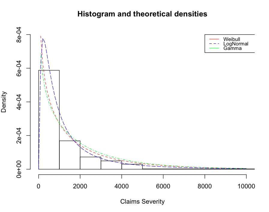
Figure 3: Histogram and theoretical densities of gamma, lognormal, and Weibull distributions for average severity data. Parameters used to generate the plot are estimated by using the “fitdist” function in the R package fitdistrplus (see more details in [55]).

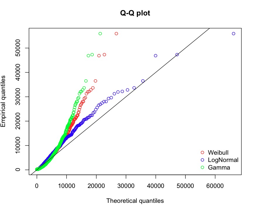
Figure 4: Q-Q plot of gamma, lognormal, and Weibull distributions for average severity data. Parameters of the distributions are estimated by using the “fitdist” function in the R package fitdistrplus (see more details in [55]).

For average severity modeling, we consider a subset of the data with $N>0$. Among all 67,856 policies, 4,624 policies satisfy this requirement (3,699 in the training data, and 925 in the test data). We calculate the average severity by dividing the total claim amount by the number of claims for each policyholder. A numerical summary of the average severity data is displayed in Table 14, indicating that the average severity data exhibit right-skewness and heavy tails. We start with some exploratory analysis, fitting gamma, lognormal and Weibull distributions to the whole data. From Figures 3 and 4 we see that all distributions can capture the right-skewed feature, however, none of them correctly captures the heavy right tail of the distribution. It appears that the lognormal distribution fits slightly better when the data are treated as IID. However, as we will see below the lognormal distribution will not be the best choice in the BCART models for this data.

For comparison, we first run some benchmark CART models. We have tried to fit the ANOVA-CART using both the original and log-transformed training data. Neither of them gives us any reasonable result since no split is identified, resulting in only a root node tree. We use the R package distRforest (cf. [56]) to fit Gamma-CART and LN-CART and both of the trees, after cost-complexity pruning, have 5 terminal nodes. As far as we are aware there is no R package with the Weibull distribution implemented for regression trees.

We then apply the proposed Gamma-BCART, LN-BCART, and Weib-BCART to the same data. The DICs in Table 15 indicate that all these BCART models choose a tree with 4 terminal nodes.

Table 15: Hyper-parameters, $p_{D}$ and DIC on training data (dataCar), and model performance on test data for average severity models with bold entries determined by DIC. The number in brackets after the abbreviation of the model indicates the number of terminal nodes for this tree.

	Training data				Test data
Model	$\gamma$	$\rho$	$p_{D}$	DIC	RSS($\bm{S}$) $\times 10^{-10}$	SE	DS	Lift
Gamma-GLM	-	-	-	-	1.4335	-	-	-
Gamma-CART (5)	-	-	-	-	1.4173	464	0.00171	1.625
LN-CART (5)	-	-	-	-	1.4168	458	0.00168	1.629
Gamma-BCART (3)	0.99	4	5.97	78061	1.4201	486	0.00181	1.567
Gamma-BCART (4)	0.99	3.5	7.97	77779	1.4176	457	0.00154	1.615
Gamma-BCART (5)	0.99	2	9.95	77982	1.4158	472	0.00167	1.643
LN-BCART (3)	0.99	5	5.97	78022	1.4193	483	0.00178	1.570
LN-BCART (4)	0.99	4	7.97	77741	1.4171	449	0.00149	1.628
LN-BCART (5)	0.99	3	9.96	77893	1.4153	456	0.00161	1.649
Weib-BCART (3)	0.99	7	5.98	77932	1.4177	473	0.00164	1.604
Weib-BCART (4)	0.99	5	7.98	77646	1.4154	433	0.00131	1.661
Weib-BCART (5)	0.99	4	9.98	77821	1.4136	446	0.00144	1.693

We also examine the splitting rules used in each tree. Gamma-CART uses both “agecat” and “veh_value” twice, with the first one being “agecat”. In contrast, LN-CART uses three different variables, “veh_value” first, followed by “veh_body” and “area”. All trees from BCART models, i.e., Gamma-BCART, LN-BCART, and Weib-BCART, have the same tree structure and splitting variables (“agecat”, “veh_value”, and “area”), while the split values/categories are slightly different. Weib-BCART, in particular, can identify a more risky group (i.e., the one with estimated average severity equal to 2743.41); see Figure 5. This may be because, as discussed in Section 3.1.2, Weib-BCART can flexibly control the shape parameter to adapt to data with different tail characteristics, allowing it to handle cases where some groups (terminal nodes) have lighter tails, and others have heavier tails. In Figure 6, we observe that although all shape parameters are smaller than one, indicating heavy tails for average severity data within each terminal node, the selected Weib-BCART tree shows improved data fitting compared to Figure 4. Similar improvements are obtained from Gamma-BCART and LN-BCART (with their Q-Q plots not shown here). We also use a standard Gamma-GLM for this dataset. We find that only the variable “gender” is significant, and thus no interaction is considered in the Gamma-GLM. Interestingly, “gender” does not appear in any of the CART and BCART models. In summary, though the variables used for different models may differ, there seems to be a consensus that “agecat” is still significantly important for average severity modeling, as Gamma-CART and all BCART models use it in the first split, and “veh_value” is another relatively important variable. This observation aligns, to some extent, with our initial analysis of the relationship between covariates and average severity; see Table 18 below. Particularly, in comparison to CARTs, BCART models reveal another important variable, “area”.

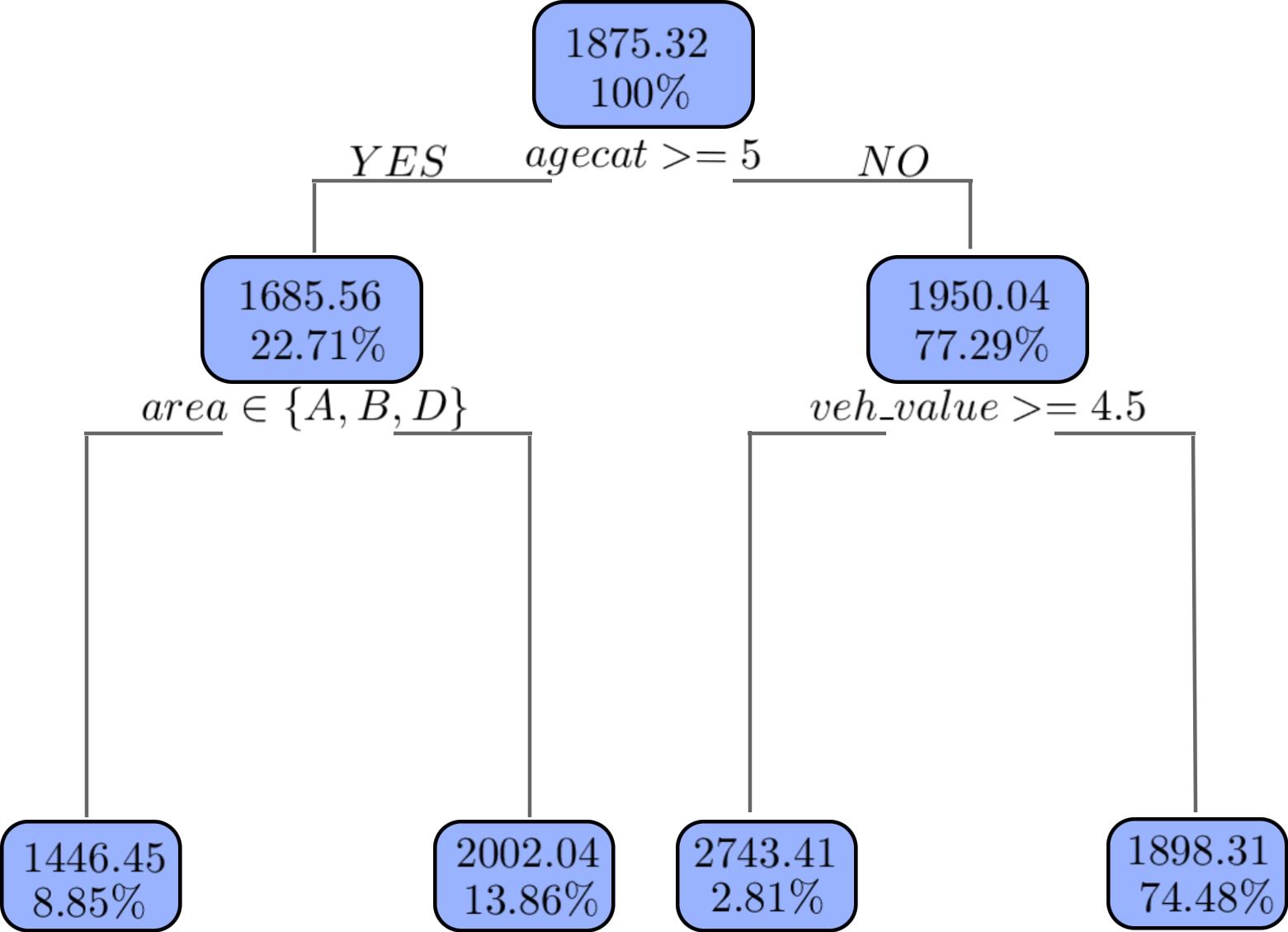
Figure 5: Optimal tree from Weib-BCART. Numbers at each node give the estimated average severity and the percentage of observations.

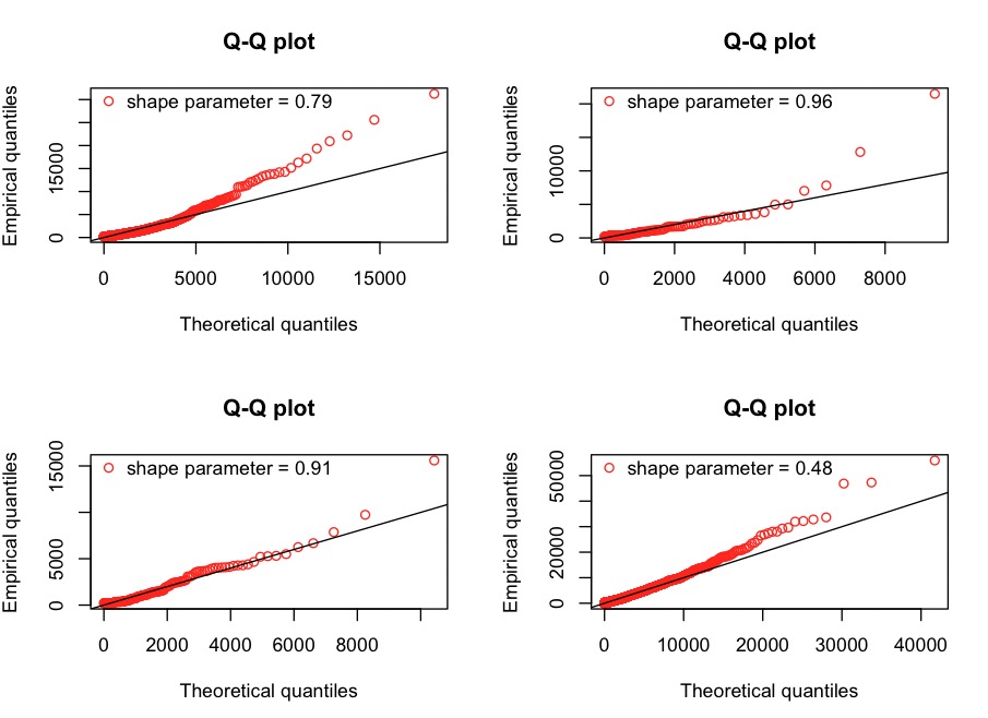
Figure 6: Q-Q plots of the Weibull distribution for average severity data in each terminal node of the optimal Weib-BCART tree. The shape parameter used to generate the plot is estimated by using MME (see Table 3 in Section 3.1.2), and the scale parameter is estimated using the posterior distribution (see Appendix A).

The performance on the test data of the selected tree models above is given in Table 15. It is evident that the Gamma-GLM is not as good as the tree models, as reflected in RSS($\bm{S}$). The study yields the following model ranking: Weib-BCART, LN-BCART, Gamma-BCART, LN-CART, Gamma-CART. This ranking is consistent with our expectations. First, it is common that average severity data is heavy-tailed. Second, the Weibull distribution is advantageous, because it can effectively handle varying tail characteristics in different tree nodes.

5.2 Aggregate claim modeling

5.2.1 Model fitting and comparison

We now fit the three BCART models with aggregate claim data, namely, frequency-severity models, sequential models, and joint models. For frequency-severity models, numerous combinations of claim frequency and average severity models are possible; see [24] for the frequency models and Section 5.1 for average severity models. Here, we choose ZIP2-BCART and Weib-BCART as the optimal tree models for frequency-severity models (see [24] and Section 5.1). Note that although ZIP2-BCART and Weib-BCART are identified as the best for claim frequency and average severity separately, it is unclear whether they remain optimal when combined. This will be examined and discussed below. For joint models, we discuss the CPG-BCART model and three types of ZICPG-BART models. Because of these choices, we also include the frequency-severity BCART model with Poisson and gamma distributions for comparison. For sequential BCART models, we consider Poisson-BCART (or called P-BCART) and ZIP2-BCART for claim frequency. Subsequently, we treat the claim count $N$ (or $\hat{N}$) as a covariate in the corresponding Gamma-BCART and Weib-BCART for average severity. The resulting models are called Gamma1-BCART (or Gamma2-BCART, with $\hat{N}$ from P-BCART) and Weib1-BCART (or Weib2-BCART, with $\hat{N}$ from ZIP2-BCART).

Table 16 presents the DICs for the average severity part in the sequential models and for the joint models. We see that in the average severity modeling with $N$ (or $\hat{N}$) as a covariate, all of them choose an optimal tree with 4 terminal nodes. Upon inspecting the tree structure, $N$ (or $\hat{N}$) is indeed used in the first step in all those optimal trees. All of them replace the previously used variable “agecat” by the covariate $N$ (or $\hat{N}$). We suspect this may be due to a strong relationship between the covariates $N$ and “agecat”, as verified in the claim frequency analysis (see [24]). Furthermore, by comparing the DICs of all Gamma-BCART and Weib-BCART models in Tables 15 and 16 (with/without $N$ or $\hat{N}$ as a covariate), we find that the model performance improves when considering $N$ (or $\hat{N}$) as a covariate, especially when using $\hat{N}$. For joint models, i.e., CPG-BCART and three ZICPG-BCART models, all of them choose optimal trees with 5 terminal nodes. Among them, ZICPG3-BCART, with the smallest DIC ($=102120$), is deemed to be the best.

Table 16: Hyper-parameters, $p_{D}$ and DIC on training data (dataCar) for aggregate claim models. The number in brackets after the abbreviation of the model indicates the number of terminal nodes for this tree. The Gamma1/Weib1 and Gamma2/Weib2 models treat the claim count $N$ and $\hat{N}$ as a covariate respectively, where $\hat{N}$ for Gamma2 comes from P-BCART and that for Weib2 comes from ZIP2-BCART. Bold font indicates DIC selected model.

Model	$\gamma$	$\rho$	$p_{D}$	DIC
Gamma1-BCART (3)	0.99	4	5.97	78032
Gamma1-BCART (4)	0.99	3.5	7.97	77750
Gamma1-BCART (5)	0.99	2	9.96	77854
Gamma2-BCART (3)	0.99	4	5.98	78024
Gamma2-BCART (4)	0.99	3.5	7.97	77743
Gamma2-BCART (5)	0.99	2	9.97	77849
Weib1-BCART (3)	0.99	7	5.98	77911
Weib1-BCART (4)	0.99	5	7.98	77619
Weib1-BCART (5)	0.99	4	9.98	77804
Weib2-BCART (3)	0.99	7	5.98	77893
Weib2-BCART (4)	0.99	5	7.98	77608
Weib2-BCART (5)	0.99	4	9.98	77787
CPG-BCART (4)	0.99	10	11.96	105710
CPG-BCART (5)	0.99	8	14.93	105626
CPG-BCART (6)	0.99	7	17.92	105643
ZICPG1-BCART (4)	0.99	11	15.97	102314
ZICPG1-BCART (5)	0.99	10	19.95	102198
ZICPG1-BCART (6)	0.99	7.5	23.92	102225
ZICPG2-BCART (4)	0.99	12	15.95	102265
ZICPG2-BCART (5)	0.99	11	19.94	102134
ZICPG2-BCART (6)	0.99	8	23.92	102167
ZICPG3-BCART (4)	0.99	14	15.94	102247
ZICPG3-BCART (5)	0.99	12	19.93	102120
ZICPG3-BCART (6)	0.99	9	23.90	102158

We again examine the splitting rules used in the selected trees. All models use the same splitting variables (“agecat”, “veh_value”, “veh_body”, and “area”), but the order of use and the tree structures vary. Notably, “agecat” is consistently the first variable. Among them, ZICPG3-BCART demonstrates the ability to identify a riskier group (i.e., the one with an estimated pure premium equal to 657.45; see Figure 7), possibly due to the same reason as discussed in [24] for the outstanding performance of ZIP2-BCART for claim frequency. Besides, we observe that the tree structure of ZICPG3-BCART is quite similar to ZIP2-BCART. However, ZICPG3-BCART identifies another important variable “area”, which was recognized as important for average severity before (see Section 5.1). We also fit a CPG-GLM to the data. We find that only the variable “agecat” is significant, aligning with its consistent selection as the first splitting variable in almost all the BCART models. It is also worth mentioning that CART is not included in this analysis due to the absence of R packages that can directly use CPG (or ZICPG) to process the data.

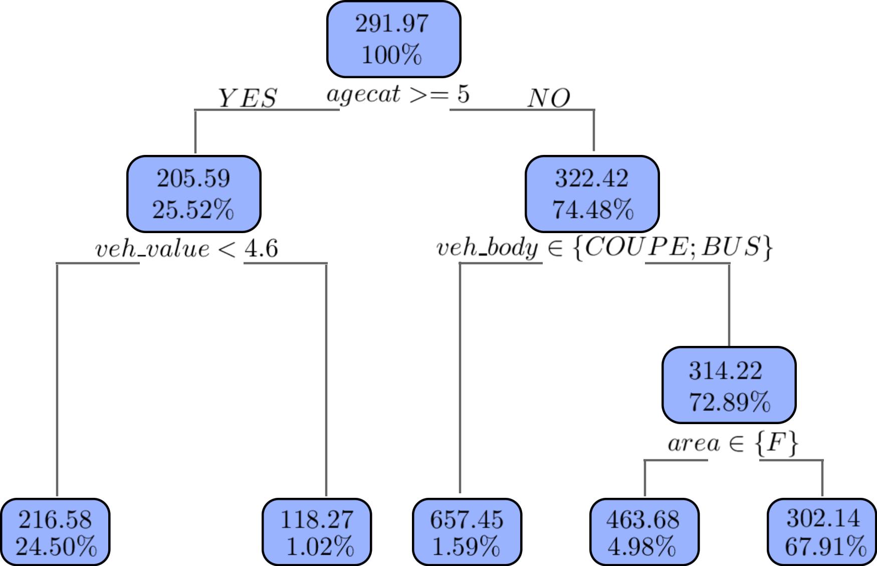
Figure 7: Optimal tree from ZICPG3-BCART. Numbers at each node give the estimated premium and the percentage of observations.

The performance of the selected trees for the test data is given in Table 17. As before, GLM exhibits poorer performance compared to tree models, as evidenced by RSS($\bm{S}$). We discuss the three types of aggregate claim models from various perspectives. The meaning of the abbreviations can be found in the captions of Tables 16–17.

Table 17: Model performance on test data (dataCar) for aggregate claim models with bold entries determined by DIC (see Table 16). $\text{F}_{\text{P}}\text{S}_{\text{G}}$ denotes frequency-severity models using Poisson and gamma distributions separately; other abbreviations can be explained similarly referring to Table 16. The number in brackets after the abbreviation of the model indicates the number of terminal nodes for those trees.

Model	RSS ($\bm{S}$)$\times 10^{-10}$	SE	DS $\times 10^{4}$	Lift
CPG-GLM	1.5187	-	-	-
$\text{F}_{\text{P}}\text{S}_{\text{G}}$-BCART (5/4)	1.4874	242.12	8.32	2.532
$\text{F}_{\text{P}}\text{S}_{\text{G1}}$-BCART (5/4)	1.4813	238.14	8.19	2.538
$\text{F}_{\text{P}}\text{S}_{\text{G2}}$-BCART (5/4)	1.4798	237.29	8.16	2.540
$\text{F}_{\text{ZIP2}}\text{S}_{\text{Weib}}$-BCART (5/4)	1.4844	240.89	8.27	2.534
$\text{F}_{\text{ZIP2}}\text{S}_{\text{Weib1}}$-BCART (5/4)	1.4790	237.01	8.14	2.541
$\text{F}_{\text{ZIP2}}\text{S}_{\text{Weib2}}$-BCART (5/4)	1.4779	236.45	8.09	2.544
CPG-BCART (4)	1.4791	237.42	8.15	2.542
CPG-BCART (5)	1.4781	235.98	7.93	2.547
CPG-BCART (6)	1.4778	236.29	8.02	2.549
ZICPG1-BCART (4)	1.4670	232.87	7.85	2.560
ZICPG1-BCART (5)	1.4497	229.73	7.56	2.584
ZICPG1-BCART (6)	1.4478	231.35	7.79	2.587
ZICPG2-BCART (4)	1.4612	232.15	7.81	2.563
ZICPG2-BCART (5)	1.4434	229.41	7.52	2.595
ZICPG2-BCART (6)	1.4417	231.10	7.77	2.597
ZICPG3-BCART (4)	1.4598	231.24	7.79	2.570
ZICPG3-BCART (5)	1.4415	228.88	7.45	2.601
ZICPG3-BCART (6)	1.4409	229.53	7.69	2.604

1. A comparison of our frequency-severity models suggests using the combination of two best models for claim frequency and average severity respectively based on all evaluation metrics, i.e., $\text{F}_{\text{ZIP2}}\text{S}_{\text{Weib}}$-BCART $>$ $\text{F}_{\text{P}}\text{S}_{\text{G}}$-BCART. In the sequential models, the same conclusion as in Section 4.1 is reached: using the estimate of the claim count $\hat{N}$ is superior to using $N$ itself when treating them as a covariate in the average severity tree. Regarding joint models, ZICPG models outperform the CPG model, with ZICPG3-BCART being the best.

2. When comparing frequency-severity models and sequential models, it is evident that adding $N$ (or $\hat{N}$) as a covariate improves performance, as shown by all evaluation metrics, i.e., $\text{F}_{\text{P}}\text{S}_{\text{G2}}$-BCART $>$ $\text{F}_{\text{P}}\text{S}_{\text{G1}}$-BCART $>$ $\text{F}_{\text{P}}\text{S}_{\text{G}}$-BCART. The same ranking is observed for another combination, i.e., $\text{F}_{\text{ZIP2}}\text{S}_{\text{Weib2}}$-BCART $>$ $\text{F}_{\text{ZIP2}}\text{S}_{\text{Weib1}}$-BCART $>$ $\text{F}_{\text{ZIP2}}\text{S}_{\text{Weib}}$-BCART. This is reasonable, as real data often exhibit a negative conditional correlation between the number of claims and average severity, favouring sequential models that consider this correlation over frequency-severity models assuming independence.

3. In comparing frequency-severity models and joint models, all evaluation metrics indicate that the optimal CPG-BCART (or ZICPG-BCART) chosen by DIC consistently outperforms frequency-severity models, suggesting that sharing information is beneficial for this dataset, i.e., one joint tree exhibits better performance. Exploration of the reasons is provided below.

4. As for sequential models and joint models, they address dependence in different ways. The former uses two trees, treating the number of claims (or its estimate) as a covariate in average severity modeling to address the dependence issue. In contrast, the latter uses one joint tree, potentially hiding some dependence in the common variables used to split the nodes and incorporating the number of claims as a model weight in the aggregate claim amount distribution. Joint models employing ZICPG distributions perform better than all the sequential models as demonstrated by all evaluation metrics, possibly due to a small negative conditional correlation between the number of claims and average severity ($-0.0336$) and the dataset involving a high proportion of zeros (93.19%).

5.2.2 Information sharing - why is it beneficial?

From the above data analysis, we have seen the advantages of being able to share information between claim frequency and severity (through common covariates in the tree) in the joint modeling of this dataset. In this section, we will further investigate the superior performance of the joint models by looking at the correlation between covariates and claim frequency and average severity.

The correlation coefficients are displayed in Table 18. Note that some of the covariates are categorical, for which we use some transformations to replace them with numerical values for the correlation calculation; see Appendix C for further details. For claim frequency, variables with the strongest correlation coefficients include “agecat” and “veh_value” which are used in the tree selected by the frequency BCART models in [24]. For average severity, we observe the same two variables exhibit the strongest correlation. Furthermore,“veh_age” has the third strongest correlation, but the selected average severity tree (cf. Figure 5) does not include it. We suspect this is due to a strong relationship between covariates “veh_age” and “veh_value” (validated in Figure 8 in Appendix C), and thus one of them is dropped to avoid multicollinearity. Additionally, both claim frequency and average severity show the strongest correlation with “agecat” which is the first splitting variable in the selected optimal frequency, average severity and joint trees, illustrating the effectiveness of BCART models for variable selection. The above discussion suggests that some common covariates exhibit strong relationships with both claim frequency and average severity, it is thus beneficial to share this information using joint modeling. This validates the conclusion of Section 5.2.1.

Table 18: Correlation coefficients between covariates (numerical ones and transformed categorical ones) and claim frequency and average severity. Bold font indicates the largest correlation coefficient (though generally small) in each row.

	veh_value	veh_age	agecat	veh_body	gender	area
Claim frequency	$-0.0047$	$0.0013$	$-0.0131$	$0.0022$	$0.0008$	$-0.0021$
Average severity	$0.0135$	$-0.0059$	$-0.0274$	$-0.0035$	$0.0003$	$-0.0034$

Next, we consider ARI (see Section 3.4) to assess the similarity between different trees and determine whether information sharing is necessary; see Table 19. As discussed in Section 4.2, although a specific threshold of ARI for making a direct judgment about the necessity for information sharing is unknown, it is evident that ARI values between all claim frequency and average severity trees are greater than 0.5. This suggests that significant intrinsic similarities of these models cannot be ignored. This also validates the preference of adopting a joint model from Section 5.2.1.

Table 19: Values of ARI between different trees. The number in brackets after the abbreviation of the model indicates the number of terminal nodes.

	Poisson-BCART (5)	ZIP2-BCART (5)	Gamma-BCART (4)	Weib-BCART (4)	CPG-BCART (5)	ZICPG3-BCART (5)
Poisson-BCART (5)	1	0.7396	0.5398	0.5163	0.8585	0.7823
ZIP2-BCART (5)	-	1	0.5599	0.5179	0.8587	0.8152
Gamma-BCART (4)	-	-	1	0.7430	0.6921	0.6423
Weib-BCART (4)	-	-	-	1	0.6491	0.6022
CPG-BCART (5)	-	-	-	-	1	0.6351
ZICPG3-BCART (5)	-	-	-	-	-	1

After conducting a thorough analysis of this dataset, we suggest that insurers need to pay more attention to policyholders who are younger and have vehicles with higher values since they are more likely to have higher risks.

Remark 5

We have also applied the proposed BCART models to other datasets (dataOhlsson included in the library insuranceData in R, freMTPL2freq and freMTPL2sev included in the library CASdatasets; see more details in [57]). Due to the similarity in analysis methods and the consistency of conclusions, we omit the details.

6 Summary

This work develops BCART models for insurance pricing, building upon the foundation of previous claim frequency analysis (see [24]). In particular, for average severity, we incorporated BCART models with gamma, lognormal, and Weibull distributions, which have different abilities to handle data with varying tail characteristics. We found that the Weib-BCART performs better than Gamma-BCART or LN-BCART since it can deal with cases where some groups have lighter tails, while others have heavier tails. Besides, in the comparison between Gamma-BCART and LN-BCART, the former is preferable for data with a lighter tail and the latter is more suitable for data with a heavier tail. This finding provides us with a practical strategy for choosing models. Concerning aggregate claim modeling, we proposed three types of models. First, we found that the sequential models treating the number of claims (or its estimate) as a covariate in the average severity modeling perform better than the standard frequency-severity models when the underlying true dependence between the number of claims and average severity is stronger. Second, we explored the choice between using two trees or one joint tree. In particular, when there are indeed common covariates affecting claim frequency and average severity and there is a relatively large amount of data available, it may be beneficial to use one joint tree, which supports the conclusion in [28] by illuminating the benefits of information sharing. Third, we provided details of evaluation metrics in the case of two trees and proposed the use of ARI to quantify the similarity between two trees, which can assist in explaining the necessity of information sharing. Finally, in the analysis of various joint models, especially the three ZICPG models employing different ways to embed exposure, we found that ZICPG3-BCART, which embeds exposure in both the zero mass component and Poisson component, delivers the most favourable results in real insurance data. We address their similarities to the analysis of ZIP models discussed in [24]. Furthermore, we introduced a more general MCMC algorithm for BCART models. These enhancements extend the applicability of BCART models to a broader range of applications.

Appendix: A

This appendix includes some technical calculations involved in Section 3.1.2. For terminal node $t$ $(t=1,2,\ldots,b)$, we denote the associated data as $(\bm{X}_{t},\bm{\bar{S}_{t}})=(({\color[rgb]{0,0,0}\bm{x}_{t1}},\bar{S}_{t1}),\ldots,(\bm{x}_{t\bar{n}_{t}},\bar{S}_{t\bar{n}_{t}}))^{\top}$.

Gamma model

The calculations for the Gamma model are similar to those in Section 3.1.1. The parameter $\alpha_{t}$ is estimated upfront by using MME through (9),

$$\hat{\alpha}_{t}=\frac{(\bar{S})_{t}^{2}}{\text{Var}(\bar{S})_{t}},$$

where $(\bar{S})_{t}$ and $\text{Var}(\bar{S})_{t}$ repectively denote the empirical mean and variance of the average severity in node $t$. Given a Gamma$(\alpha_{\pi},\beta_{\pi})$ prior for $\beta_{t}$, the integrated likelihood for terminal node $t$ is

$$p_{\text{G}}\left(\bm{\bar{S}}_{t}\mid\bm{X}_{t},\hat{\alpha}_{t}\right) =\int_{0}^{\infty}f_{\text{G}}\left(\bm{\bar{S}}_{t}\mid\hat{\alpha}_{t},\beta_{t}\right)p(\beta_{t})d\beta_{t}$$

$$=\int_{0}^{\infty}\prod_{i=1}^{\bar{n}_{t}}\left(\frac{\beta_{t}^{\hat{\alpha}_{t}}\bar{S}_{ti}^{\hat{\alpha}_{t}-1}e^{-\beta_{t}\bar{S}_{ti}}}{\Gamma(\hat{\alpha}_{t})}\right)\frac{\beta_{\pi}^{\alpha_{\pi}}{\beta_{t}}^{\alpha_{\pi}-1}e^{-\beta_{\pi}\beta_{t}}}{\Gamma(\alpha_{\pi})}d\beta_{t}$$

$$=\frac{\beta_{\pi}^{\alpha_{\pi}}\prod_{i=1}^{\bar{n}_{t}}\bar{S}_{ti}^{\hat{\alpha}_{t}-1}}{\Gamma(\alpha_{\pi}){\color[rgb]{0,0,0}\Gamma(\hat{\alpha}_{t})^{\bar{n}_{t}}}}\frac{\Gamma(\bar{n}_{t}\hat{\alpha}_{t}+\alpha_{\pi})}{(\sum_{i=1}^{\bar{n}_{t}}\bar{S}_{ti}+\beta_{\pi})^{\bar{n}_{t}\hat{\alpha}_{t}+\alpha_{\pi}}}.$$

From the above equation, we obtain

$$\beta_{t}\mid\bm{\bar{S}}_{t},\zzz{\hat{\alpha}_{t}}\ \ \sim\ \ \text{Gamma}\left(\bar{n}_{t}\hat{\alpha}_{t}+\alpha_{\pi},\sum_{i=1}^{\bar{n}_{t}}\bar{S}_{ti}+\beta_{\pi}\right).$$

The integrated likelihood for the tree $\mathcal{T}$ is thus given by

$$p_{\text{G}}\left(\bm{\bar{S}}\mid\bm{X},\bm{\hat{\alpha}},\mathcal{T}\right)=\prod_{t=1}^{b}p_{\text{G}}\left(\bm{\bar{S}}_{t}\mid\bm{X}_{t},\hat{\alpha}_{t}\right).$$

Similarly to Section 3.1.1, the DIC_t for terminal node $t$ is defined as $\mathrm{DIC}_{t}=D(\bar{\beta}_{t})+2p_{Dt}$, where the posterior mean for $\beta_{t}$ is given by

$$\bar{\beta}_{t}=\frac{\bar{n}_{t}\hat{\alpha}_{t}+\alpha_{\pi}}{\sum_{i=1}^{{\color[rgb]{0,0,0}\bar{n}}_{t}}\bar{S}_{ti}+\beta_{\pi}}{\color[rgb]{0,0,0};}$$

the goodness-of-fit is defined by

$$D(\bar{\beta}_{t}) =-2\sum_{i=1}^{{\color[rgb]{0,0,0}\bar{n}}_{t}}\log f_{\text{G}}(\bar{S}_{ti}\mid\hat{\alpha}_{t},\bar{\beta}_{t})$$

$$=-2\sum_{i=1}^{{\color[rgb]{0,0,0}\bar{n}}_{t}}\left[\hat{\alpha}_{t}\log(\bar{\beta}_{t})+(\hat{\alpha}_{t}-1)\log(\bar{S}_{ti})-\bar{\beta}_{t}\bar{S}_{ti}-\log\left(\Gamma(\hat{\alpha}_{t})\right)\right],$$

and the effective number of parameters $p_{Dt}$ is given by

$$p_{Dt} =1+2\sum_{i=1}^{{\color[rgb]{0,0,0}\bar{n}}_{t}}\left\{\log\left(f_{\text{G}}(\bar{S}_{ti}\mid\hat{\alpha}_{t},\bar{\beta}_{t})\right)-\mathbb{E}_{\text{post}}\left(\log\left(f_{\text{G}}(\bar{S}_{ti}\mid\hat{\alpha}_{t},\beta_{t})\right)\right)\right\}$$

$$=1+2\left(\log\left({\color[rgb]{0,0,0}\bar{n}}_{t}\hat{\alpha}_{t}+\alpha_{\pi}\right)-\psi\left({\color[rgb]{0,0,0}\bar{n}}_{t}\hat{\alpha}_{t}+\alpha_{\pi}\right)\right){\color[rgb]{0,0,0}\bar{n}}_{t}\hat{\alpha}_{t}.$$

Thus,

$$\text{DIC}_{t} = D(\bar{\beta}_{t})+2p_{Dt}$$

$$= -2\sum_{i=1}^{{\color[rgb]{0,0,0}\bar{n}}_{t}}\left(\hat{\alpha}_{t}\log\left(\frac{{\color[rgb]{0,0,0}\bar{n}}_{t}\hat{\alpha}_{t}+\alpha_{\pi}}{\sum_{i=1}^{{\color[rgb]{0,0,0}\bar{n}}_{t}}\bar{S}_{ti}+\beta_{\pi}}\right)+(\hat{\alpha}_{t}-1)\log(\bar{S}_{ti})-\frac{{\color[rgb]{0,0,0}\bar{n}}_{t}\hat{\alpha}_{t}+\alpha_{\pi}}{\sum_{i=1}^{{\color[rgb]{0,0,0}\bar{n}}_{t}}\bar{S}_{ti}+\beta_{\pi}}\bar{S}_{ti}\right)$$

$$\ \ \ ~{}~{}+2\bar{n}_{t}\left[\log\left(\Gamma(\hat{\alpha}_{t})\right)\right]+2+4\left(\log\left({\color[rgb]{0,0,0}\bar{n}}_{t}\hat{\alpha}_{t}+\alpha_{\pi}\right)-\psi\left({\color[rgb]{0,0,0}\bar{n}}_{t}\hat{\alpha}_{t}+\alpha_{\pi}\right)\right){\color[rgb]{0,0,0}\bar{n}}_{t}\hat{\alpha}_{t}.$$

Lognormal model

To obtain $\sigma_{t}$ upfront, we use the MME to solve the equations involving the empirical mean and variance given in Table 2, i.e.,

$$(\bar{S})_{t}=e^{\zzz{\mu_{t}}+\zzz{\sigma_{t}^{2}}/2},\ \ \text{Var}(\bar{S})_{t}=\left(e^{\zzz{\sigma_{t}^{2}}}-1\right)e^{2\zzz{\mu_{t}}+\zzz{\sigma_{t}^{2}}}.$$

Since there is no explicit solution for it, we use the package optimx in software R to solve this problem; see more details in [58]. With the assumed Normal($\mu_{\pi},\sigma_{\pi}^{2}$) prior for $\mu_{t}$ and the estimated parameter $\hat{\sigma}_{t}$, we can obtain

$$\log{\color[rgb]{0,0,0}\left({\color[rgb]{0,0,0}f_{\text{LN}}\left(\bm{\bar{S}}_{t}\mid\mu_{t},\hat{\sigma}_{t}\right)p(\mu_{t})}\right)}$$

$$=-\sum_{i=1}^{\bar{n}_{t}}\log\bar{S}_{ti}-\frac{\bar{n}_{t}}{2}\log(2\pi\hat{\sigma}_{t}^{2})-\frac{1}{2\hat{\sigma}_{t}^{2}}\sum_{i=1}^{\bar{n}_{t}}\left(\log\bar{S}_{ti}-\mu_{t}\right)^{2}-\frac{1}{2}\log(2\pi\sigma_{\pi}^{2})-\frac{\left(\mu_{t}-\mu_{\pi}\right)^{2}}{2\sigma_{\pi}^{2}}$$

$$=-\sum_{i=1}^{\bar{n}_{t}}\log\bar{S}_{ti}-\frac{\bar{n}_{t}}{2}\log(2\pi\hat{\sigma}_{t}^{2})-\frac{1}{2\hat{\sigma}_{t}^{2}}\left(\sum_{i=1}^{\bar{n}_{t}}\left(\log\bar{S}_{ti}\right)^{2}-2\mu_{t}\sum_{i=1}^{\bar{n}_{t}}\log\bar{S}_{ti}+\bar{n}_{t}\mu_{t}^{2}\right)$$

$$\ \ \ \ -\frac{1}{2}\log(2\pi\sigma_{\pi}^{2})-\frac{1}{2\sigma_{\pi}^{2}}(\mu_{t}^{2}-2\mu_{t}\mu_{\pi}+\mu_{\pi}^{2})$$

$$=-\sum_{i=1}^{\bar{n}_{t}}\log\bar{S}_{ti}-\frac{\bar{n}_{t}}{2}\log(2\pi\hat{\sigma}_{t}^{2})-\frac{1}{2}\log(2\pi\sigma_{\pi}^{2})-\frac{1}{2\hat{\sigma}_{t}^{2}}\sum_{i=1}^{\bar{n}_{t}}\left(\log\bar{S}_{ti}\right)^{2}-\frac{1}{2\sigma_{\pi}^{2}}\mu_{\pi}^{2}-\frac{1}{2\sigma_{*t}^{2}}\left(\mu_{t}-\mu_{*t}\right)^{2}$$

with

$$\sigma_{*t}^{2}=\frac{\hat{\sigma}_{t}^{2}\sigma_{\pi}^{2}}{\bar{n}_{t}\sigma_{\pi}^{2}+\hat{\sigma}_{t}^{2}},$$

$$\mu_{*t}=\frac{\hat{\sigma}_{t}^{2}}{\bar{n}_{t}\sigma_{\pi}^{2}+\hat{\sigma}_{t}^{2}}\mu_{\pi}+\frac{\bar{n}_{t}\sigma_{\pi}^{2}}{\bar{n}_{t}\sigma_{\pi}^{2}+\hat{\sigma}_{t}^{2}}\frac{1}{\bar{n}_{t}}\sum_{i=1}^{\bar{n}_{t}}\log\bar{S}_{ti}=\sigma_{*t}^{2}\left(\frac{\mu_{\pi}}{\sigma_{\pi}^{2}}+\frac{\sum_{i=1}^{\bar{n}_{t}}\log\bar{S}_{ti}}{\hat{\sigma}_{t}^{2}}\right).$$

Subsequently, we can derive

$${\color[rgb]{0,0,0}f_{\text{LN}}\left(\bm{\bar{S}}_{t}\mid\mu_{t},\hat{\sigma}_{t}\right)p(\mu_{t})}$$

$$=\exp\left(-\sum_{i=1}^{\bar{n}_{t}}\log\bar{S}_{ti}-\frac{\bar{n}_{t}}{2}\log(2\pi\hat{\sigma}_{t}^{2})-\frac{1}{2}\log(2\pi\sigma_{\pi}^{2})-\frac{1}{2\hat{\sigma}_{t}^{2}}\sum_{i=1}^{\bar{n}_{t}}\left(\log\bar{S}_{ti}\right)^{2}-\frac{1}{2\sigma_{\pi}^{2}}\mu_{\pi}^{2}-\frac{1}{2\sigma_{*t}^{2}}\left(\mu_{t}-\mu_{*t}\right)^{2}\right)$$

$$=\left(\prod_{i=1}^{\bar{n}_{t}}\bar{S}_{ti}^{-1}\right)(2\pi\hat{\sigma}_{t}^{2})^{-\frac{\bar{n}_{t}}{2}}(2\pi\sigma_{\pi}^{2})^{-\frac{1}{2}}\exp\left(-\frac{1}{2\hat{\sigma}_{t}^{2}}\sum_{i=1}^{\bar{n}_{t}}\left(\log\bar{S}_{ti}\right)^{2}\right)\exp\left(-\frac{1}{2\sigma_{\pi}^{2}}\mu_{\pi}^{2}\right)\exp\left(-\frac{1}{2\sigma_{*t}^{2}}\left(\mu_{t}-\mu_{*t}\right)^{2}\right).$$

Thereafter, the integrated likelihood for terminal node $t$ can be obtained as

$$p_{\text{LN}}\left(\bm{\bar{S}}_{t}\mid\bm{X}_{t}\right)$$

$$=\int_{-\infty}^{\infty}f_{\text{LN}}\left(\bm{\bar{S}}_{t}\mid\mu_{t},\hat{\sigma}_{t}\right)p(\mu_{t})d\mu_{t}$$

$$=\frac{1}{{\color[rgb]{0,0,0}\hat{\sigma}_{t}^{\bar{n}_{t}}}\sigma_{\pi}{(2\pi)}^{(\zzz{{\color[rgb]{0,0,0}\bar{n}}_{t}+1})/2}\prod_{i=1}^{\bar{n}_{t}}\bar{S}_{ti}}\exp\left(-\frac{1}{2\hat{\sigma}_{t}^{2}}\sum_{i=1}^{\bar{n}_{t}}\left(\log\bar{S}_{ti}\right)^{2}\right)\exp\left(-\frac{1}{2\sigma_{\pi}^{2}}\mu_{\pi}^{2}\right)\int_{-\infty}^{\infty}\exp\left(-\frac{1}{2\sigma_{*t}^{2}}\left(\mu_{t}-\mu_{*t}\right)^{2}\right)d\mu_{t}$$

$$=\zzz{\frac{\sigma_{*t}}{\hat{\sigma}_{t}^{\bar{n}_{t}}\sigma_{\pi}{(2\pi)}^{\zzz{\bar{n}_{t}}/2}\prod_{i=1}^{\bar{n}_{t}}\bar{S}_{ti}}}\exp\left(-\frac{1}{2\hat{\sigma}_{t}^{2}}\sum_{i=1}^{\bar{n}_{t}}\left(\log\bar{S}_{ti}\right)^{2}\right)\exp\left(-\frac{1}{2\sigma_{\pi}^{2}}\mu_{\pi}^{2}\right).$$

Clearly, from the above equation, we have

$$\mu_{t}\mid\bm{\bar{S}}_{t},\hat{\sigma}_{t}\ \ \sim\ \ \text{Normal}\left(\sigma_{*t}^{2}\left(\frac{\mu_{\pi}}{\sigma_{\pi}^{2}}+\frac{\sum_{i=1}^{\bar{n}_{t}}\log(\bar{S}_{ti})}{\hat{\sigma}_{t}^{2}}\right),\frac{\hat{\sigma}_{t}^{2}\sigma_{\pi}^{2}}{\bar{n}_{t}\sigma_{\pi}^{2}+\hat{\sigma}_{t}^{2}}\right).$$

The integrated likelihood for the tree $\mathcal{T}$ is thus given by $p_{\text{LN}}\left(\bm{\bar{S}}\mid\bm{X},\bm{\hat{\sigma}},\mathcal{T}\right)=\prod_{t=1}^{b}p_{\text{LN}}\left(\bm{\bar{S}}_{t}\mid\bm{X}_{t},\hat{\sigma}_{t}\right).$ Next, $\mathrm{DIC}_{t}=D(\bar{\mu}_{t})+2p_{Dt},$ where

$$D\left(\bar{\mu}_{t}\right) = -2\sum_{i=1}^{\bar{n}_{t}}\log f_{\text{LN}}(\bar{S}_{ti}\mid\bar{\mu}_{t},\hat{\sigma}_{t})$$

$$= -2\sum_{i=1}^{\bar{n}_{t}}\left(-\frac{(\log(\bar{S}_{ti})-\bar{\mu}_{t})^{2}}{2\hat{\sigma}_{t}^{2}}-\log\left(\bar{S}_{ti}\hat{\sigma}_{t}\sqrt{2\pi}\right)\right),$$

with

$$\bar{\mu}_{t}=\mu_{*t}=\sigma_{*t}^{2}\left(\frac{\mu_{\pi}}{\sigma_{\pi}^{2}}+\frac{\sum_{i=1}^{\bar{n}_{t}}\log(\bar{S}_{ti})}{\hat{\sigma}_{t}^{2}}\right),$$

and the effective number of parameters $p_{Dt}$ is given by

$$p_{Dt} =1+2\sum_{i=1}^{{\color[rgb]{0,0,0}\bar{n}}_{t}}\left\{\log(f_{\text{LN}}(\bar{S}_{ti}\mid\bar{\mu}_{t},\hat{\sigma}_{t})-\mathbb{E}_{\text{post}}\left(\log\left(f_{\text{LN}}(\bar{S}_{ti}\mid\mu_{t},\hat{\sigma}_{t})\right)\right)\right\}$$

$$=1+\sum_{i=1}^{{\color[rgb]{0,0,0}\bar{n}}_{t}}\frac{\sigma_{*t}^{2}}{\hat{\sigma}_{t}^{2}}=1+\frac{{\color[rgb]{0,0,0}\bar{n}}_{t}\sigma_{\pi}^{2}}{{\color[rgb]{0,0,0}\bar{n}}_{t}\sigma_{\pi}^{2}+\hat{\sigma}_{t}^{2}},$$

and thus

$$\text{DIC}_{t} = D\left(\bar{\mu}_{t}\right)+2p_{Dt}$$

$$= -2\sum_{i=1}^{{\color[rgb]{0,0,0}\bar{n}}_{t}}\left(-\frac{\left(\log(\bar{S}_{ti})-\bar{\mu}_{t}\right)^{2}}{2\hat{\sigma}_{t}^{2}}-\log\left(\bar{S}_{ti}\hat{\sigma}_{t}\sqrt{2\pi}\right)\right)+2+\frac{2{\color[rgb]{0,0,0}\bar{n}}_{t}\sigma_{\pi}^{2}}{{\color[rgb]{0,0,0}\bar{n}}_{t}\sigma_{\pi}^{2}+\hat{\sigma}_{t}^{2}}.$$

Weibull model

Similarly to the lognormal distribution, to obtain $\alpha_{t}$ upfront, we need to solve

$$(\bar{S})_{t}=\beta^{\zzz{1/\alpha}}\Gamma(1+1/\alpha),\ \ \text{Var}(\bar{S})_{t}=\beta^{\zzz{2/\alpha}}\left[\Gamma(1+2/\alpha)-\left(\Gamma(1+1/\alpha)\right)^{2}\right],$$

and will use the package optimx in software R. With the inverse-gamma prior in (15) and the estimated parameter $\hat{\alpha}_{t}$, the integrated likelihood for terminal node $t$ can be obtained as

$$p_{\text{Weib}}\left(\bm{\bar{S}}_{t}\mid\bm{X}_{t}\right) =\int_{0}^{\infty}f_{\text{Weib}}\left(\bm{\bar{S}}_{t}\mid\hat{\alpha}_{t},\beta_{t}\right)p(\beta_{t})d\beta_{t}$$

$$=\frac{\beta_{\pi}^{\alpha_{\pi}}{\color[rgb]{0,0,0}\hat{\alpha}_{t}^{\bar{n}_{t}}}\prod_{i=1}^{\bar{n}_{t}}\bar{S}_{ti}^{\hat{\alpha}_{t}-1}}{\Gamma(\alpha_{\pi})}\frac{\Gamma(\bar{n}_{t}+\alpha_{\pi})}{(\sum_{i=1}^{\bar{n}_{t}}\bar{S}_{ti}^{\hat{\alpha}_{t}}+\beta_{\pi})^{\bar{n}_{t}+\alpha_{\pi}}}.$$

Clearly, we have

$$\beta_{t}\mid\bm{\bar{S}}_{t}\ \ \sim\ \ \text{Inverse-Gamma}\left(\bar{n}_{t}+\alpha_{\pi},\sum_{i=1}^{\bar{n}_{t}}\bar{S}_{ti}^{\hat{\alpha}_{t}}+\beta_{\pi}\right).$$

The integrated likelihood for the tree $\mathcal{T}$ is thus given by $p_{\text{Weib}}\left(\bm{\bar{S}}\mid\bm{X},\bm{\hat{\alpha}},\mathcal{T}\right)=\prod_{t=1}^{b}p_{\text{Weib}}\left(\bm{\bar{S}}_{t}\mid\bm{X}_{t},\hat{\alpha}_{t}\right).$ Next, $\mathrm{DIC}_{t}=D(\bar{\beta}_{t})+2p_{Dt},$ where

$$D(\bar{\beta}_{t}) = -2\sum_{i=1}^{\bar{n}_{t}}\log f_{\text{Weib}}(\bar{S}_{ti}\mid\hat{\alpha}_{t},\bar{\beta}_{t})$$

$$= -2\sum_{i=1}^{\bar{n}_{t}}\left(\log(\hat{\alpha}_{t})-\log(\bar{\beta}_{t})+(\hat{\alpha}_{t}-1)\log(\bar{S}_{ti})-\bar{S}_{ti}^{\hat{\alpha}_{t}}/\bar{\beta}_{t}\right),$$

with

$$\bar{\beta}_{t}=\frac{\sum_{i=1}^{\bar{n}_{t}}\bar{S}_{ti}^{\hat{\alpha}_{t}}+\beta_{\pi}}{\bar{n}_{t}+\alpha_{\pi}-1},$$

and the effective number of parameters $p_{Dt}$ is given by

$$p_{Dt} =1+2\sum_{i=1}^{\bar{n}_{t}}\left\{\log(f_{\text{Weib}}(\bar{S}_{ti}\mid\hat{\alpha}_{t},\bar{\beta}_{t})-\mathbb{E}_{\text{post}}\left(\log\left(f_{\text{Weib}}(\bar{S}_{ti}\mid\hat{\alpha}_{t},\beta_{t})\right)\right)\right\}$$

$$=1+2\sum_{i=1}^{\bar{n}_{t}}\left(\log(\bar{n}_{t}+\alpha_{\pi}-1)-\psi(\bar{n}_{t}+\alpha_{\pi})+\frac{\bar{S}_{ti}^{\hat{\alpha}_{t}}}{\sum_{i=1}^{\bar{n}_{t}}\bar{S}_{ti}^{\hat{\alpha}_{t}}+\beta_{\pi}}\right),$$

where we use the fact that

$$\mathbb{E}_{\text{post}}\left(\log(\beta_{t})\right)=\log\left(\sum_{i=1}^{\bar{n}_{t}}\bar{S}_{ti}^{\hat{\alpha}_{t}}+\beta_{\pi}\right)-\psi(\bar{n}_{t}+\alpha_{\pi})$$

and

$$\mathbb{E}_{\text{post}}\left(1/\beta_{t}\right)=\frac{\bar{n}_{t}+\alpha_{\pi}}{\sum_{i=1}^{\bar{n}_{t}}\bar{S}_{ti}^{\hat{\alpha}_{t}}+\beta_{\pi}}.$$

Thus,

$$\text{DIC}_{t} =D(\bar{\beta}_{t})+2p_{Dt}$$

$$=-2\sum_{i=1}^{\bar{n}_{t}}\left(\log(\hat{\alpha}_{t})-\log(\bar{\beta}_{t})+(\hat{\alpha}_{t}-1)\log(\bar{S}_{ti})-\bar{S}_{ti}^{\hat{\alpha}_{t}}/\bar{\beta}_{t}\right)$$

$$\ \ \ +2+4\sum_{i=1}^{\bar{n}_{t}}\left(\log(\bar{n}_{t}+\alpha_{\pi}-1)-\psi(\bar{n}_{t}+\alpha_{\pi})+\frac{\bar{S}_{ti}^{\hat{\alpha}_{t}}}{\sum_{i=1}^{\bar{n}_{t}}\bar{S}_{ti}^{\hat{\alpha}_{t}}+\beta_{\pi}}\right).$$

Appendix: B

In this appendix, we show that (20) is the marginal distribution of (21). We will discuss two cases $N_{ti}>0$ and $N_{ti}=0$, respectively.

Case $N_{ti}>0$. By definition, this entails $\delta_{ti}=1$. Thus,

$$f_{\text{ZICPG}}\left(N_{ti},S_{ti},0,\phi_{ti}\mid\mu_{t},\lambda_{t},\alpha_{t},\beta_{t}\right)=0,$$

and

$$f_{\text{ZICPG}}(N_{ti},S_{ti},1,\phi_{ti}\mid\mu_{t},\lambda_{t},\alpha_{t},\beta_{t})=e^{-\phi_{ti}(1+\mu_{t}w_{ti})}\left(\frac{\mu_{t}w_{ti}\left(\lambda_{t}u_{ti}\right)^{N_{ti}}}{N_{ti}!}e^{-\lambda_{t}u_{ti}}\right)\frac{\beta_{t}^{N_{ti}\alpha_{t}}S_{ti}^{N_{ti}\alpha{{}_{t}}-1}e^{-\beta_{t}S_{ti}}}{\Gamma(N_{ti}\alpha{{}_{t}})}.$$

Integrating with respect to $\phi_{ti}$, we obtain

$$\int_{0}^{\infty}f_{\text{ZICPG}}\left(N_{ti},S_{ti},1,\phi_{ti}\mid\mu_{t},\lambda_{t},\alpha_{t},\beta_{t}\right)d\phi_{ti}$$

$$=\left(\frac{\mu_{t}w_{ti}\left(\lambda_{t}u_{ti}\right)^{N_{ti}}}{N_{ti}!}e^{-\lambda_{t}u_{ti}}\right)\frac{\beta_{t}^{N_{ti}\alpha_{t}}S_{ti}^{N_{ti}\alpha{{}_{t}}-1}e^{-\beta_{t}S_{ti}}}{\Gamma(N_{ti}\alpha{{}_{t}})}\int_{0}^{\infty}e^{-\phi_{ti}(1+\mu_{t}w_{ti})}d\phi_{ti}$$

$$=\left(\frac{\mu_{t}w_{ti}\left(\lambda_{t}u_{ti}\right)^{N_{ti}}}{N_{ti}!}e^{-\lambda_{t}u_{ti}}\right)\frac{\beta_{t}^{N_{ti}\alpha_{t}}S_{ti}^{N_{ti}\alpha{{}_{t}}-1}e^{-\beta_{t}S_{ti}}}{\Gamma(N_{ti}\alpha{{}_{t}})}\frac{1}{1+\mu_{t}w_{ti}},$$

which gives the expression of ZICPG model in (20) when $N_{ti}>0$.

Case $N_{ti}=0$. With $\delta_{ti}=0$, we know

$$f_{\text{ZICPG}}\left(0,0,0,\phi_{ti}\mid\mu_{t},\lambda_{t},\alpha_{t},\beta_{t}\right)=e^{-\phi_{ti}(1+\mu_{t}w_{ti})},$$

and thus

$$\int_{0}^{\infty}f_{\text{ZICPG}}\left(0,0,0,\phi_{ti}\mid\mu_{t},\lambda_{t},\alpha_{t},\beta_{t}\right)d\phi_{ti}=\int_{0}^{\infty}e^{-\phi_{ti}(1+\mu_{t}w_{ti})}d\phi_{ti}=\frac{1}{1+\mu_{t}w_{ti}}.$$

With $\delta_{ti}=1$, we have

$$f_{\text{ZICPG}}\left(0,0,1,\phi_{ti}\mid\mu_{t},\lambda_{t},\alpha_{t},\beta_{t}\right)=e^{-\phi_{ti}(1+\mu_{t}w_{ti})}\mu_{t}w_{ti}e^{-\lambda_{t}u_{ti}},$$

and thus

$$\int_{0}^{\infty}f_{\text{ZICPG}}\left(0,0,1,\phi_{ti}\mid\mu_{t},\lambda_{t},\alpha_{t},\beta_{t}\right)d\phi_{ti}$$

$$=\mu_{t}w_{ti}e^{-\lambda_{t}u_{ti}}\int_{0}^{\infty}e^{-\phi_{ti}(1+\mu_{t}w_{ti})}d\phi_{ti}=e^{-\lambda_{t}u_{ti}}\frac{\mu_{t}w_{ti}}{1+\mu_{t}w_{ti}}.$$

Summing up over $\delta_{ti}$, we obtain

$$f_{\text{ZICPG}}\left(0,0\mid\mu_{t},\lambda_{t},\alpha_{t},\beta_{t}\right)=\frac{1}{1+\mu_{t}w_{ti}}+\frac{\mu_{t}w_{ti}}{1+\mu_{t}w_{ti}}e^{-\lambda_{t}u_{ti}},$$

which gives the expression of ZICPG model in (20) when $N_{ti}=0$.

Appendix: C

In this appendix, we explain the numerical transformation of categorical covariates that was implemented in the BCART models and used in the calculations of correlation coefficient (see Table 18). The numerical transformation of categorical covariates employs the idea that was implemented in CART. When processing categorical variables, we calculate empirical claim frequency (or average severity) for each categorical level as a numerical replacement. In detail, at each node and for each categorical variable, we gather data at every level. Using these collections, the empirical claim frequency can be calculated as the ratio of sum of claim counts and sum of exposure. Similarly, the empirical average severity can be determined by the ratio of sum of aggregate claim amounts and sum of claim counts. As an illustration, Table 20 presents the empirical claim frequency and average severity of the categorical variable on training data at the root node. In our proposed BCART models, the numerical transformation was done after each split, in each updated node. The relationship between covariates “veh_value” and “veh_age” is provided in Figure 8. More details can be found in [44].

Table 20: Empirical claim frequency and average severity for different vehicle body levels on training data (dataCar) at the root node. Bold font indicates the smallest and largest values for frequency and average severity calculated separately.

Vehicle body level	Frequency	Average severity
CONVT	0.092	2296
UTE	0.131	2164
MIBUS	0.142	2580
HBACK	0.151	1947
SEDAN	0.153	1678
TRUCK	0.154	2458
STNWG	0.163	1894
PANVN	0.166	1958
HDTOP	0.174	2168
COUPE	0.235	2503
MCARA	0.253	712
RDSTR	0.257	456
BUS	0.387	1336

Figure 8: Scatter plot between vehicle age and vehicle value after logarithmic transformation on training data (dataCar).

References

• [1] M.V. Wuthrich and M. Merz “Statistical Foundations of Actuarial Learning and its Applications” Springer Actuarial, https://link.springer.com/book/10.1007/978-3-031-12409-9, 2022
• [2] Roel Henckaerts, Marie-Pier Côté, Katrien Antonio and Roel Verbelen “Boosting insights in insurance tariff plans with tree-based machine learning methods” In North American Actuarial Journal 25 Taylor & Francis, 2021, pp. 255–285
• [3] Edward W Frees, Gee Lee and Lu Yang “Multivariate frequency-severity regression models in insurance” In Risks 4 MDPI, 2016, pp. 4
• [4] Gee Y Lee and Peng Shi “A dependent frequency-severity approach to modeling longitudinal insurance claims” In Insurance: Mathematics and Economics 87 Elsevier, 2019, pp. 115–129
• [5] Peng Shi and Zifeng Zhao “Regression for copula-linked compound distributions with applications in modeling aggregate insurance claims” In The Annals of Applied Statistics 14 JSTOR, 2020, pp. 357–380
• [6] Peter X-K Song, Mingyao Li and Ying Yuan “Joint regression analysis of correlated data using Gaussian copulas” In Biometrics 65 Wiley Online Library, 2009, pp. 60–68
• [7] Guangyuan Gao and Jiahong Li “Dependence modeling of frequency-severity of insurance claims using waiting time” In Insurance: Mathematics and Economics 109 Elsevier, 2023, pp. 29–51
• [8] Michael Stanley Smith “Bayesian approaches to copula modelling” In arXiv preprint arXiv:1112.4204, 2011
• [9] Michael S Smith and Mohamad A Khaled “Estimation of copula models with discrete margins via Bayesian data augmentation” In Journal of the American Statistical Association 107 Taylor & Francis, 2012, pp. 290–303
• [10] Claudia Czado, Rainer Kastenmeier, Eike Christian Brechmann and Aleksey Min “A mixed copula model for insurance claims and claim sizes” In Scandinavian Actuarial Journal 2012 Taylor & Francis, 2012, pp. 278–305
• [11] Peng Shi, Xiaoping Feng and Anastasia Ivantsova “Dependent frequency-severity modeling of insurance claims” In Insurance: Mathematics and Economics 64 Elsevier, 2015, pp. 417–428
• [12] Woojoo Lee, Sojung C Park and Jae Youn Ahn “Investigating dependence between frequency and severity via simple generalized linear models” In Journal of the Korean Statistical Society 48 Elsevier, 2019, pp. 13–28
• [13] Edward W Frees, Jie Gao and Marjorie A Rosenberg “Predicting the frequency and amount of health care expenditures” In North American Actuarial Journal 15 Taylor & Francis, 2011, pp. 377–392
• [14] José Garrido, Christian Genest and Juliana Schulz “Generalized linear models for dependent frequency and severity of insurance claims” In Insurance: Mathematics and Economics 70 Elsevier, 2016, pp. 205–215
• [15] Bent Jørgensen and Marta C Paes De Souza “Fitting Tweedie’s compound Poisson model to insurance claims data” In Scandinavian Actuarial Journal 1994 Taylor & Francis, 1994, pp. 69–93
• [16] Oscar Alberto Quijano Xacur and José Garrido “Generalised linear models for aggregate claims: to Tweedie or not?” In European Actuarial Journal 5 Springer, 2015, pp. 181–202
• [17] Łukasz Delong, Mathias Lindholm and Mario V Wüthrich “Making Tweedie’s compound Poisson model more accessible” In European Actuarial Journal 11 Springer, 2021, pp. 185–226
• [18] Guangyuan Gao “Fitting Tweedie’s compound Poisson model to pure premium with the EM algorithm” In Insurance: Mathematics and Economics 114 Elsevier, 2024, pp. 29–42
• [19] He Zhou, Wei Qian and Yi Yang “Tweedie gradient boosting for extremely unbalanced zero-inflated data” In Communications in Statistics-Simulation and Computation 51 Taylor & Francis, 2022, pp. 5507–5529
• [20] Yi Lian et al. “A Tweedie compound Poisson model in reproducing kernel Hilbert space” In Technometrics 65 Taylor & Francis, 2023, pp. 281–295
• [21] Christopher Blier-Wong, Hélène Cossette, Luc Lamontagne and Etienne Marceau “Machine learning in P&C insurance: A review for pricing and reserving” In Risks 9 MDPI, 2020, pp. 4
• [22] Michel Denuit and Julien Trufin “Effective Statistical Learning Methods for Actuaries” Springer, 2019
• [23] Mario V. Wuthrich and Christoph Buser “Data Analytics for Non-Life Insurance Pricing (January 9, 2023).” Available at SSRN: https://ssrn.com/abstract=2870308, 2022
• [24] Yaojun Zhang, Lanpeng Ji, Georgios Aivaliotis and Charles Taylor “Bayesian CART models for insurance claims frequency” In Insurance: Mathematics and Economics 114 Elsevier, 2024, pp. 108–131
• [25] Gordon K Smyth and Bent Jørgensen “Fitting Tweedie’s compound Poisson model to insurance claims data: dispersion modelling” In ASTIN Bulletin: The Journal of the IAA 32 Cambridge University Press, 2002, pp. 143–157
• [26] Seungha Um, Antonio R. Linero, Debajyoti Sinha and Dipankar Bandyopadhyay “Bayesian Additive Regression Trees for Multivariate Responses” In Statistics in Medicine 42 Wiley, 2023, pp. 246–263 DOI: 10.1002/sim.9613
• [27] Veronika Rocková and Stephanie Van der Pas “Posterior concentration for Bayesian regression trees and forests” In Annals of Statistics 48, 2020, pp. 2108–2131
• [28] Antonio R Linero, Debajyoti Sinha and Stuart R Lipsitz “Semiparametric mixed-scale models using shared Bayesian forests” In Biometrics 76 Wiley Online Library, 2020, pp. 131–144
• [29] Hugh A Chipman, Edward I George and Robert E McCulloch “Bayesian CART model search” In Journal of the American Statistical Association 93 Taylor & Francis, 1998, pp. 935–948
• [30] David GT Denison, Bani K Mallick and Adrian FM Smith “A Bayesian CART algorithm” In Biometrika 85 Oxford University Press, 1998, pp. 363–377
• [31] Edward I George “Bayesian model selection” In Encyclopedia of Statistical Sciences Update 3 Wiley, New York, 1998
• [32] Antonio R Linero “A review of tree-based Bayesian methods” In Communications for Statistical Applications and Methods 24 The Korean Statistical Society, 2017, pp. 543–559
• [33] Jared S Murray “Log-linear Bayesian additive regression trees for multinomial Logistic and count regression models” In Journal of the American Statistical Association 116 Taylor & Francis, 2021, pp. 756–769
• [34] David J Spiegelhalter, Nicola G Best, Bradley P Carlin and Angelika Van Der Linde “Bayesian measures of model complexity and fit” In Journal of the Royal Statistical Society: Series B (Statistical Methodology) 64 Wiley Online Library, 2002, pp. 583–639
• [35] Gilles Celeux, Florence Forbes, Christian P Robert and D Mike Titterington “Deviance information criteria for missing data models” In Bayesian Aanalysis 1 International Society for Bayesian Analysis, 2006, pp. 651–673
• [36] Mario V Wuthrich “Non-life Insurance: Mathematics & Statistics” Available at SSRN 2319328, 2022
• [37] Cyprian Ondieki Omari, Shalyne Gathoni Nyambura and Joan Martha Wairimu Mwangi “Modeling the frequency and severity of auto insurance claims using statistical distributions” In Journal of Mathematical Finance, 2018
• [38] Edward W Frees, Richard A Derrig and Glenn Meyers “Predictive modeling in actuarial science” In Predictive modeling applications in actuarial science 1 Cambridge University Press, 2014, pp. 1–10
• [39] Siswadi and CP Quesenberry “Selecting among weibull, lognormal and gamma distributions using complete and censored smaples” In Naval Research Logistics Quarterly 29 Wiley Online Library, 1982, pp. 557–569
• [40] Horst Rinne “The weibull distribution: a handbook” CRC press, 2008
• [41] Daniel Fink “A compendium of conjugate priors” Accessed Online (August, 2024): https://www.johndcook.com/CompendiumOfConjugatePriors.pdf, 1997
• [42] Mert Mehmet and Yasemin Saykan “On a bonus-malus system where the claim frequency distribution is geometric and the claim severity distribution is Pareto” In Hacettepe Journal of Mathematics and Statistics 34 Hacettepe University, 2005, pp. 75–81
• [43] Sébastien Farkas, Olivier Lopez and Maud Thomas “Cyber claim analysis using Generalized Pareto regression trees with applications to insurance” In Insurance: Mathematics and Economics 98 Elsevier, 2021, pp. 92–105
• [44] Yaojun Zhang “Insurance Pricing using Bayesian Tree Models” PhD thesis, University of Leeds, 2024
• [45] Susanne Gschlößl and Claudia Czado “Spatial modelling of claim frequency and claim size in non-life insurance” In Scandinavian Actuarial Journal 2007 Taylor & Francis, 2007, pp. 202–225
• [46] Yi Yang, Wei Qian and Hui Zou “Insurance premium prediction via gradient tree-boosted Tweedie compound Poisson models” In Journal of Business & Economic Statistics 36 Taylor & Francis, 2018, pp. 456–470
• [47] Michel Denuit, Arthur Charpentier and Julien Trufin “Autocalibration and Tweedie-dominance for insurance pricing with machine learning” In Insurance: Mathematics and Economics 101 Elsevier, 2021, pp. 485–497
• [48] Esbjörn Ohlsson and Björn Johansson “Non-life Insurance Pricing with Generalized Linear Models” Springer, 2010
• [49] Tom MW Nye, Pietro Lio and Walter R Gilks “A novel algorithm and web-based tool for comparing two alternative phylogenetic trees” In Bioinformatics 22 Oxford University Press, 2006, pp. 117–119
• [50] William M Rand “Objective criteria for the evaluation of clustering methods” In Journal of the American Statistical Association 66 Taylor & Francis, 1971, pp. 846–850
• [51] Lawrence Hubert and Phipps Arabie “Comparing partitions” In Journal of Classification 2 Springer, 1985, pp. 193–218
• [52] Alexander J Gates and Yong-Yeol Ahn “The impact of random models on clustering similarity” In arXiv preprint arXiv:1701.06508, 2017
• [53] Matthew J. Vavrek “fossil: Palaeoecological and Palaeogeographical Analysis Tools” R package version 0.4.0, 2020 URL: https://CRAN.R-project.org/package=fossil
• [54] Alicja Wolny–Dominiak and Michal Trzesiok “insuranceData: a collection of Insurance Datasets Useful in Risk Classification in Non-life insurance” R package version 1.0, 2014 URL: https://CRAN.R-project.org/package=insuranceData
• [55] Christophe Dutang Marie-Laure Delignette-Muller and Regis Pouillot “fitdistrplus: help to Fit of a Parametric Distribution to Non-Censored or Censored Data” R package version 1.1-11, 2023 URL: https://CRAN.R-project.org/package=fitdistrplus
• [56] Roel Henckaerts “distRforest: random Forests with Distribution-Based Loss Functions”, 2020 URL: henckr.github.io/distRforest/
• [57] Arthur Charpentier “Computational Actuarial Science with R” Boca Raton, FL: CRC Press, 2014
• [58] Ravi Varadhan Nash and Gabor Grothendieck “optimx: expanded Replacement and Extension of the “optim” Function” R package version 2023-10.21, 2023 URL: https://CRAN.R-project.org/package=optimx