Quantifying predictability and basin structure in infinite-dimensional delayed systems: a stochastic basin entropy approach

Abstract

The Mackey-Glass system is a paradigmatic example of a delayed model whose dynamics is particularly complex due to, among other factors, its multistability involving the coexistence of many periodic and chaotic attractors. The prediction of the long-term dynamics is especially challenging in these systems, where the dimensionality is infinite and initial conditions must be specified as a function in a finite time interval. In this paper we extend the recently proposed basin entropy to randomly sample arbitrarily high-dimensional spaces. By complementing this stochastic approach with the basin fraction of the attractors in the initial conditions space we can understand the structure of the basins of attraction and how they are intermixed. The results reported here allow us to quantify the predictability and provide indicators of the presence of bifurcations. The tools employed can result very useful in the study of complex systems of infinite dimension.

In many real systems, ranging from climate to brain dynamics, long-term predictability is challenging due to chaotic solutions and high sensitivity to initial conditions. Multistable systems, in particular, exhibit unpredictable behavior that varies with control parameters. In these cases it is more a question of which attractor the system tends towards and not so much the value of the (local) Lyapunov exponents. Basin entropy is a new tool designed to measure predictability by partitioning initial condition spaces and analyzing their long-term dynamics. In time-delayed systems, and in particular in the Mackey-Glass system, the complexity increases as the system’s dimensionality becomes arbitrarily large, complicating the exploration of initial conditions. In earlier work, we demonstrated that basin entropy is effective even in simple time-delayed bistable systems for studying multistability and predicting bifurcations. We extend this to the Mackey-Glass model, known for its rich dynamics and multiple attractors, showing that a modified, stochastic version of basin entropy effectively characterizes the system’s behavior.

I Introduction

In nonlinear systems the predictability of the long-term dynamics is strongly limited by the presence of chaotic solutions and the high sensitivity to initial conditions. Particularly in multistable systems the predictability is not at all uniform and strongly depends on the control parameters. In this situation, the analysis of basins of attraction plays a crucial role Menck et al. (2013); Leng, Lin, and Kurths (2016); Schultz et al. (2017); Rakshit et al. (2017); Gelbrecht, Boers, and Kurths (2021); Datseris, Luiz Rossi, and Wagemakers (2023). Basin entropy is a recently proposed tool to quantify the predictability of long-term dynamics in these systems Daza et al. (2016, 2017). Its main idea consists in dividing the space of initial conditions into regular partitions and studying within each one the long time evolution of the dynamics. This tool was successfully applied in several systems such as the analysis of fractal boundaries Gusso and de Mello (2021), to classify different kinds of basins as Wada, riddled or intermingled Daza, Wagemakers, and Sanjuán (2022), or to explore bifurcations Daza, Wagemakers, and Sanjuán (2023); Wagemakers, Daza, and Sanjuán (2023). A related approach has also been proposed to study the dynamic stability of complex networks naturally composed of many nodes Halekotte and Feudel (2020); Halekotte, Vanselow, and Feudel (2021).

In systems with time delay the additional complication arises that the dimension of the system is arbitrarily large and the space of initial conditions cannot be exhaustively explored Wernecke, Sándor, and Gros (2019); Otto, Just, and Radons (2019). In a previous work Tarigo et al. (2024) we considered one of the simplest time-delayed systems, a bistable system with a delay term, which exhibits complex dynamics Erneux (2009). We showed that even in this system the basin entropy is a valid tool to study multistability and can be an indicator of the occurrence of bifurcations. Here, we consider the Mackey-Glass (MG) model, a time-delayed system that exhibits particularly rich dynamics with regions impacted by the existence of many attractors and we show that the basin entropy modified to stochastically partition the initial condition space it is useful to characterize the dynamics of the system. To complement the results obtained with this tool we also consider the basin fraction occupied by the attractors Menck et al. (2013); Leng, Lin, and Kurths (2016) in the space of initial configurations and the analysis of cross-sections obtained for particular families of initial condition functions. Our approach is based on the joint use of these three tools.

The Mackey-Glass model initially proposed for the study of physiological systems is a paradigmatic example of a time-delayed system that exhibits very complex dynamics Mackey and Glass (1977). Its dynamics is characterized by multistability that includes the coexistence of different attractors, fixed points, limit cycles or chaotic attractors Junges and Gallas (2012); Amil, Cabeza, and Marti (2015); L’Her et al. (2016). In Ref. Junges and Gallas, 2012, J. A. C. Gallas et al showed that the dynamics exhibit periodic or aperiodic oscillations where peaks appear and disappear due to continuous deformations as the control parameters vary. Bifurcation diagrams revealed the existence of a complex structure of period-doubling or peak-adding bifurcations leading to chaotic windows. They also obtained stability diagrams in terms of control parameters and effective delayed showing complex mosaics of periodic and chaotic regions. The variation of the delay time allowed them to observe some kind of lethargy with which the system responds to the change from one to many degrees of freedom, demonstrating that the emergence of high dimensionality does not instantaneously alter the dynamics of the system. This observation challenged the general validity of some analytical methods previously considered in the literature.

In general, as a consequence of time delay, it is required to specify a continuous function of initial conditions over a finite interval to determine its evolution and dimensionality results to be arbitrarily large. In a previous work we designed an electronic circuit with feedback that simulates the MG system and showed that the experimental results obtained with the circuit reproduce the behavior of the model over a wide range of parameters Amil, Cabeza, and Marti (2015). This implementation served to show that, taking arbitrary families of initial conditions, in general different attractors coexist for the same value of the control parameters. These attractors can be either fixed points, or periodic oscillations with equal amplitude maxima but different orderings, or chaotic attractors Amil et al. (2015). Additionally, hysteresis loops were identified by varying the delay parameter in bifurcation diagrams. Subsequently, we focused on precisely quantify the multistability in this system Tarigo et al. (2022). With this objective, we selected representative initial condition functions and systematically explored the parameter space counting the number of different attractors. In this way, we identified the regions in which more attractors coexist and assessed the impact of multistability. In the present work we go deeper into this subject and use the basin entropy, basin fraction, number of attractors and the way in which they are intermingled to analyze the dynamics and predictability of the system.

II The Mackey-Glass delayed model

The Mackey-Glass model is a time-delayed differential equation widely used to study complex dynamic behaviors in systems exhibiting chaos and multistability Mackey and Glass (1977). Originally proposed by Michael Mackey and Leon Glass in 1977 to describe physiological control systems, such as blood cell regulation, the model has since been applied in various fields including biology, physics, and engineering. The equation characterizes how the rate of change of a variable, such as the concentration of a substance, depends not only on its current state but also on its state at some previous time. This time delay introduces infinite-dimensional phase space, making the Mackey-Glass model a prototypical example for investigating time-delayed systems. Its ability to generate rich dynamics, including periodic, quasi-periodic, and chaotic solutions, makes it a valuable tool for exploring fundamental principles of nonlinear dynamics and chaos theory.

Let us denote $x(t)$ the concentration of a certain blood component at time $t$. The dynamics of the system can be described by means of the Mackey-Glass model in terms of the balance between a nonlinear production term and a decay term. Using dimensionless variables the model equation can be written as

$$\frac{dx}{dt}=\alpha\frac{x_{\Gamma}}{1+x_{\Gamma}^{n}}-x$$ (1)

where $x_{\Gamma}=x(t-\Gamma)$ is the delayed state variable, $\Gamma$ plays the role of an effective delay and $\alpha$ and $n$ determine the production term.

In a previous work we developed an electronic circuit that mimics the behavior of the Mackey-Glass system using specially designed electronic blocks for the nonlinear production function and to account for the time delay. An advantage of this strategy is that the discrete equation for the time evolution can be obtained in form of an explicit equation reproducing exactly the evolution equation in the continuum limit. The numerical results obtained with both the discrete map of dimension $N$ and integration methods demonstrate significant agreement with those obtained experimentally. The discrete map can be written as

$$\begin{split}x_{1}(t+1)&=e^{-\frac{\Gamma}{N}}x_{1}(t)+\Big{(}1-e^{-\frac{\Gamma}{N}}\Big{)}\alpha\frac{x_{N}(t)}{1+x^{n}_{N}(t)}\\ x_{i}(t+1)&=x_{i-1}(t)\quad\forall i=2,...,N.\end{split}$$ (2)

In this approximation the continuous-time variable $x(t)$ is approximated by $N$ continuous variables at discrete times, $x_{i}(t)$, $\forall i=1,...N$. The dynamics of $x_{1}(t)$ given by Eq. 2 reproduces the time evolution of the continuous variable by taking the value at the delayed time from the $x_{N}(t)$. The remaining units $x_{i}(t)$ for $i>1$ simply transfer their value to the adjacent variable at each time step. It can be seen that (2) converges to (1) in the continuous limit $\Delta t=\Gamma/{N}\rightarrow 0$ and that $N$ turns out to be the number of time steps for one delay unit $\Gamma$. The state space of (2) is $N$-dimensional. This discretization of (1) presents the advantage of being exact in time Amil, Cabeza, and Marti (2015) and faster to compute than other conventional methods for numerically solving DDEs. There are four control parameters in the discrete map, $n$ and $\alpha$ determine the shape of the production term, while $N$ and $\Gamma$ define the time delay. In the following sections we are going to use $n=4$ and $N=396$ unless otherwise is stated.

III Stochastic basin entropy in high dimensional systems

We begin by reviewing the definition of basin entropy for a non-delayed dynamical system with $N_{A}$ coexisting attractors Daza et al. (2016, 2017); Daza, Wagemakers, and Sanjuán (2023). To compute the basin entropy, we consider a partition of the phase space into $N_{b}$ boxes of linear size $\varepsilon$ and examine which attractor each point in each box evolves towards. We sample a large number, $L$, of trajectories much greater than the number of possible attractors inside box $i$ ($L\gg m_{i}$). This allows us to estimate the probability, $p_{ij}$, of reaching the attractor $j$ starting from an initial condition in box $i$, with the probabilities normalized so that $\sum_{j}^{m_{i}}p_{ij}=1$. The basin entropy is then defined as

$$S_{b}=-\frac{1}{N_{b}}\sum_{i=1}^{N_{b}}\sum_{j=1}^{m_{i}}p_{ij}\log p_{ij}$$ (3)

which can be identified as the Shannon entropy.

As the dimension of the phase space grows the algorithm in (3) becomes very computationally expensive and is not worth using it for high dimensional systems. This problem arises due to the fact that all the phase space must be explored in order to calculate the basin entropy. Because basin entropy is an average of the quantity $p_{ij}\log p_{ij}$ over the entire phase space, it is reasonable to postulate, following an approach similar to the Monte Carlo method, that it will converge to the average value by randomly sampling an adequate number of boxes. This method allows for a much less computational effort provided that the basin entropy converges rapidly to the average value.

In Fig. 1 we calculated the basin entropy of the system for different number of boxes and different number of trajectories per box. The center of each box was chosen randomly from a uniform distribution between $0+\varepsilon/2$ and $2-\varepsilon/2$ and then each initial condition was taken randomly inside that box. We can see that as the number of trajectories per box increases, the basin entropy starts to converge to a precise value. Also increasing the number of boxes taken, decreases the dispersion of the basin entropy around the mean value. We followed this procedure for other values of the parameters of the system, finding that the basin entropy converges before $100$ boxes and $1000$ trajectories per box in every case. In sections V and VI we use $100$ boxes and $1000$ trajectories per box to calculate basin entropy.

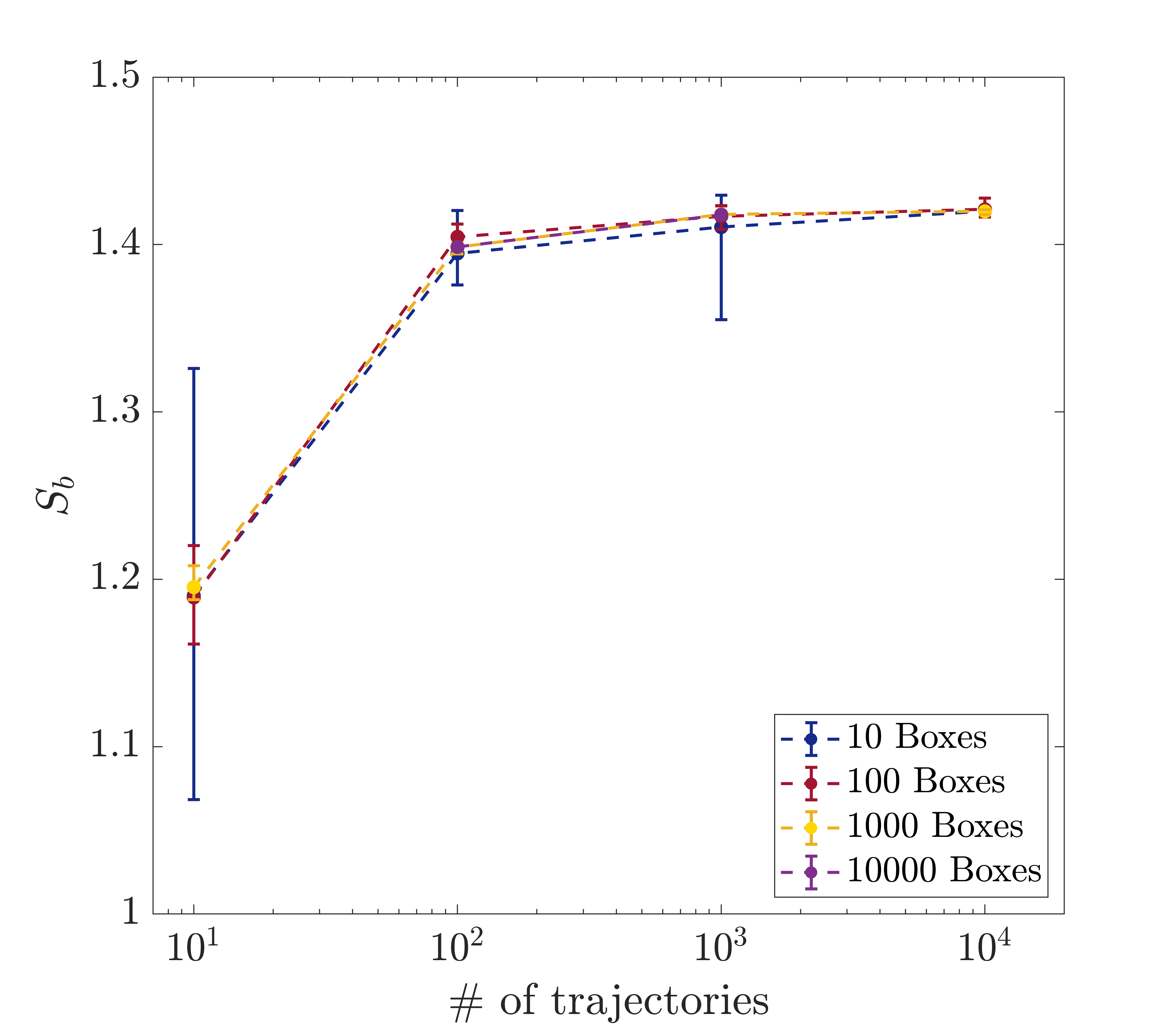
Figure 1: Convergence of basin entropy as a function of the number of initial conditions sampled per box for different number of boxes (indicated with colors in the legend box). For each point 10 iterations of the basin entropy were averaged. The symbols indicate the average value while the error bars denote the minimum and maximum values found. All points correspond to the same parameter values, $\alpha=5$, $\Gamma=18$ and $n=8$.

IV Visualizing high-dimensional sate spaces

To show the rich variety of behaviors found in the Mackey-Glass system, in Fig. 2 we present examples of stationary solutions of Eq. (2) for different parameter values and different initial conditions. Panels (a) through (d) show examples of limit cycles while panel (e) shows an example of a chaotic trajectory. We can see the multistability of the system as panels (b)-(c) and (d)-(e) in Fig. 2 correspond to the same control parameter values but different initial conditions.

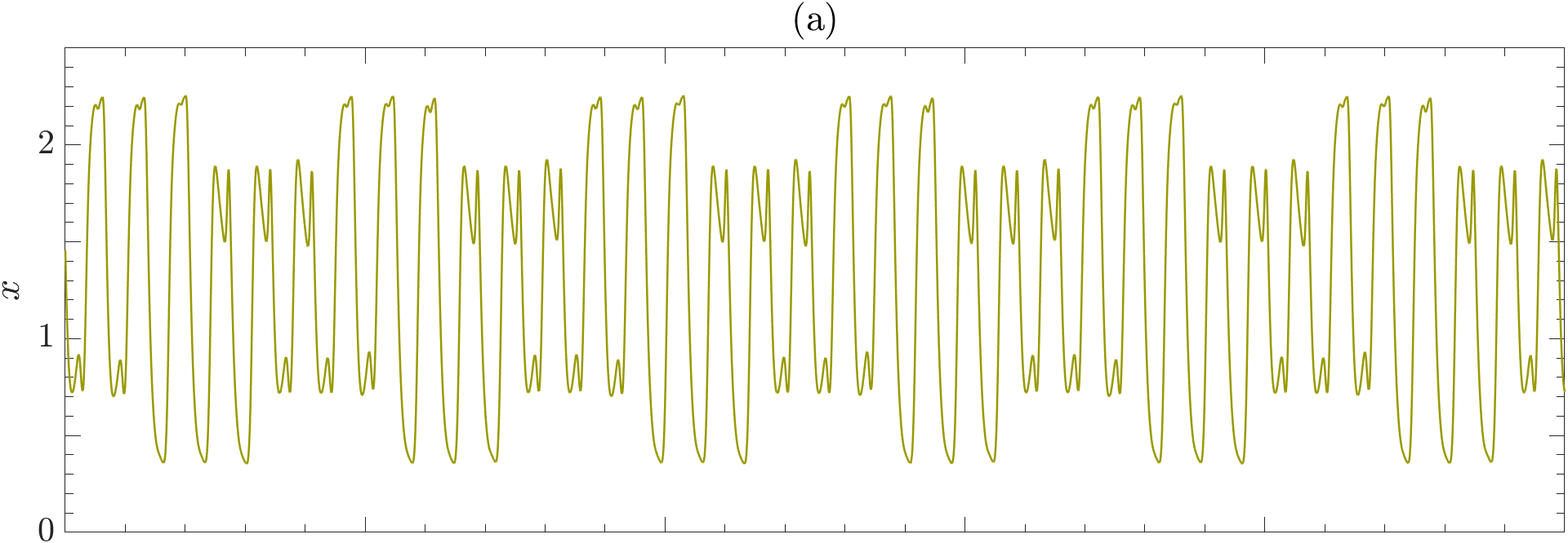
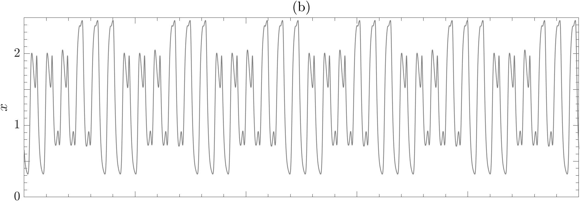
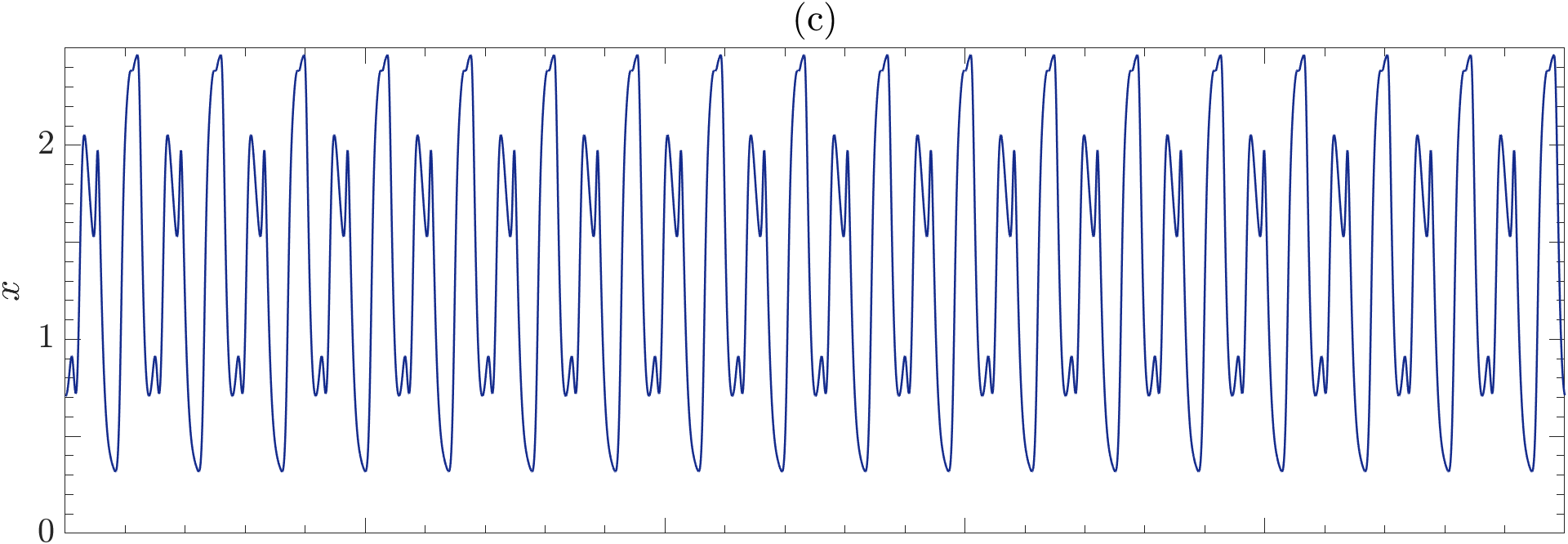
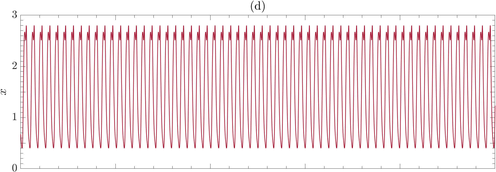
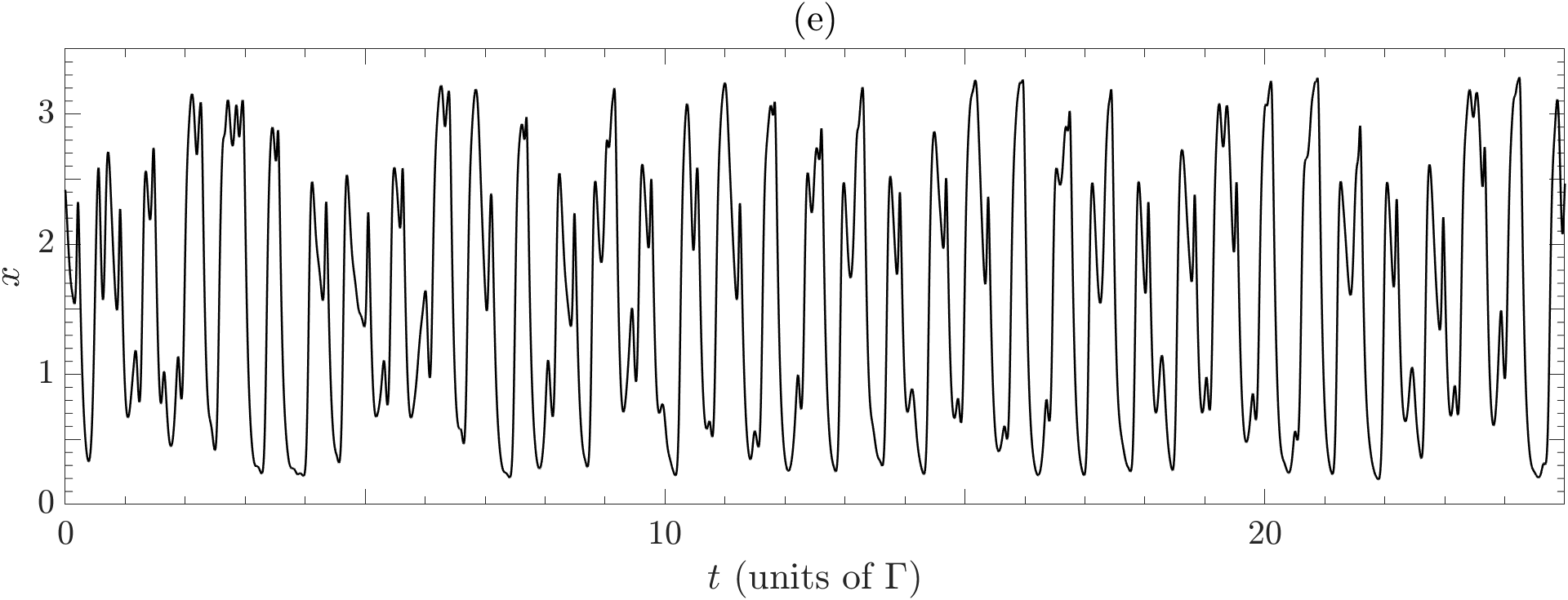
Figure 2: Representative examples of time evolution of Eq. (2). The parameters correspond to $n=4$ and $(\alpha,\Gamma)=$ $(4,19.5)$ for (a), $(4.4,17.2)$ for (b) and (c) and $(5.9,19.7)$ for (d) and (e). Initial conditions correspond to Eq. (4) with parameters values $(A,x_{off})=$ $(0.9,1.01)$ for (a), $(0.2,1.7)$ for (b), $(0.2,1.69)$ for (c), $(0.9,1.01)$ for (d) and $(0.5,1.05)$ for (e). For all solutions a transient of $1000\Gamma$ was discarded.

To further study the multistability of the system we plotted relevant cross-sections of the systems state space. Figure 3 illustrates the attractors reached for points of two-dimensional cross-sections of the state space of the system and four different pairs of parameters $\Gamma$ and $\alpha$. The color code used in Fig. 3 was chosen with the same criteria as for Fig. 2. The cross-sections correspond to the following parametric function of initial conditions

$$x_{i}^{in}=A\sin(2\pi t_{i})+x_{off},\quad t_{i}=-\frac{N-i+1}{N}\Gamma$$ (4)

where $A$ and $x_{off}$ are the parameters of this family of functions. In the diagrams of Fig. 3, we can appreciate the structural richness exhibited by the space of initial conditions. As the system’s parameters change, both the number of solutions and the nature of the boundaries separating the basins of attraction vary. In some regions, the boundaries are relatively smooth, while in others, they become increasingly intermixed as the parameters change. It is also evident that, for certain parameter values, different periodic solutions coexist, and in others, chaotic trajectories emerge.

This approach to studying multistability in delayed systems, as explored in Refs. Amil et al., 2015; Tarigo et al., 2022, 2024, offers the advantage of visualizing the basins of attraction of a high-dimensional system within a two-dimensional diagram. However, it has the drawback of being highly dependent on the specific cross-sections chosen or the family of functions used. To address this limitation, in the next section, we randomly sample the state space to count the different solutions of the system and quantify their relative importance.

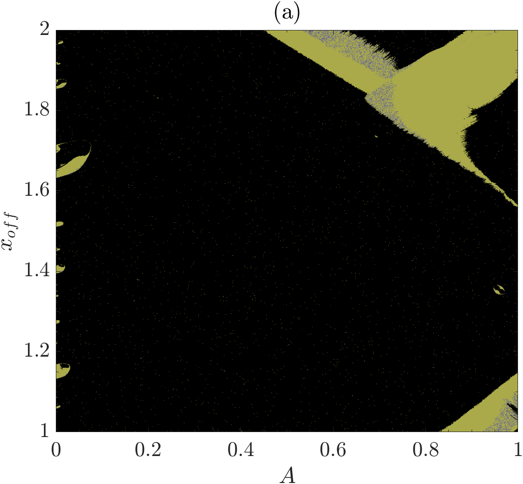
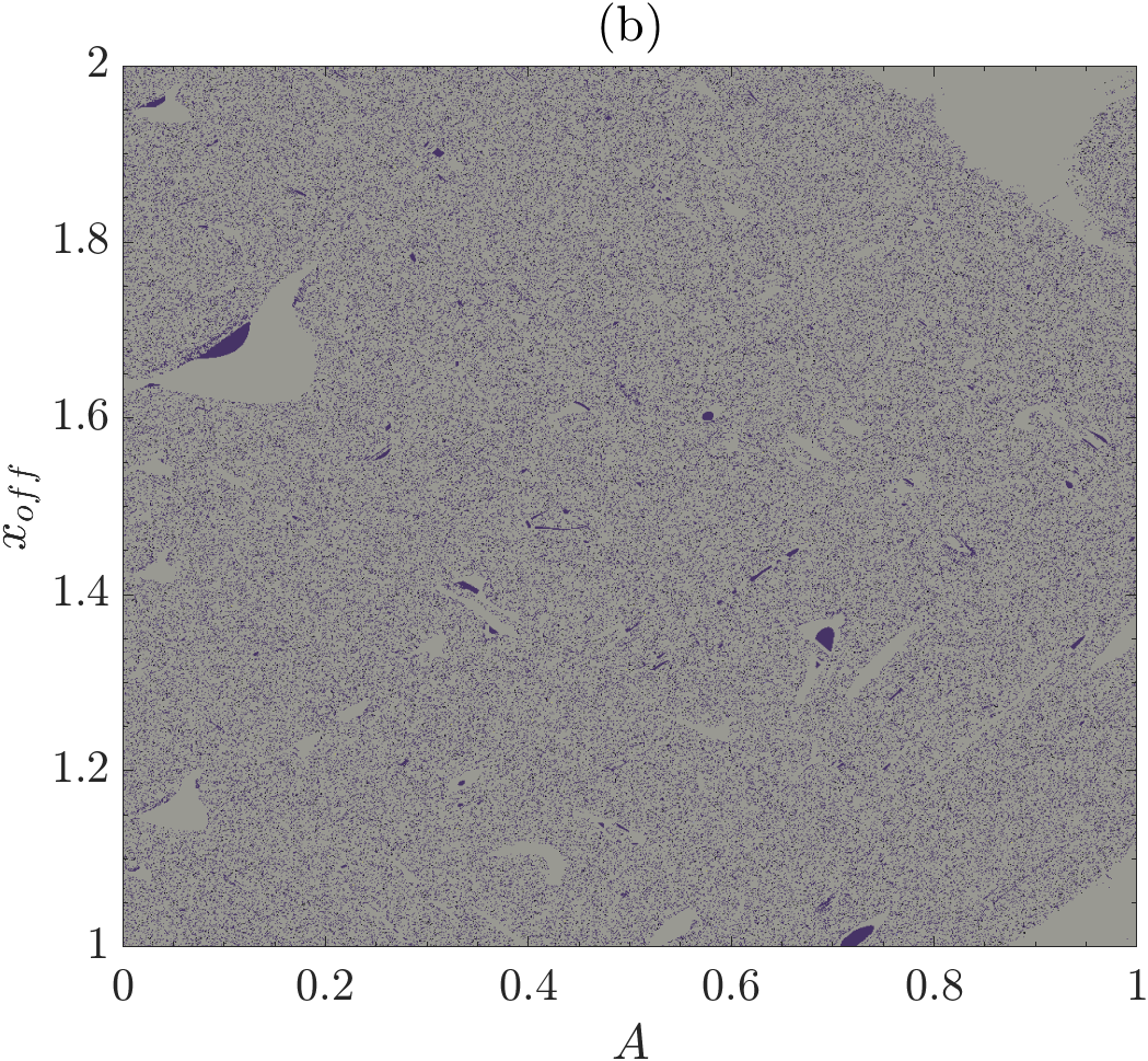
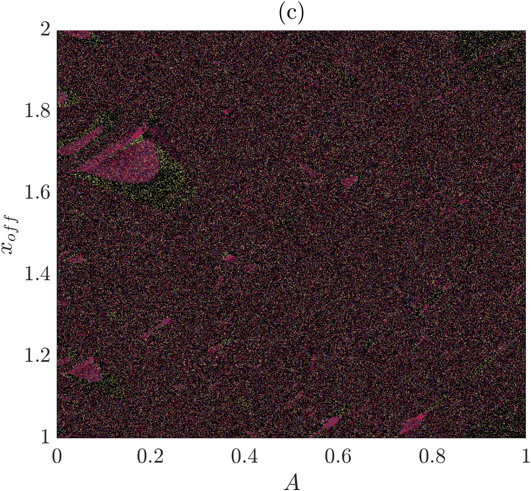
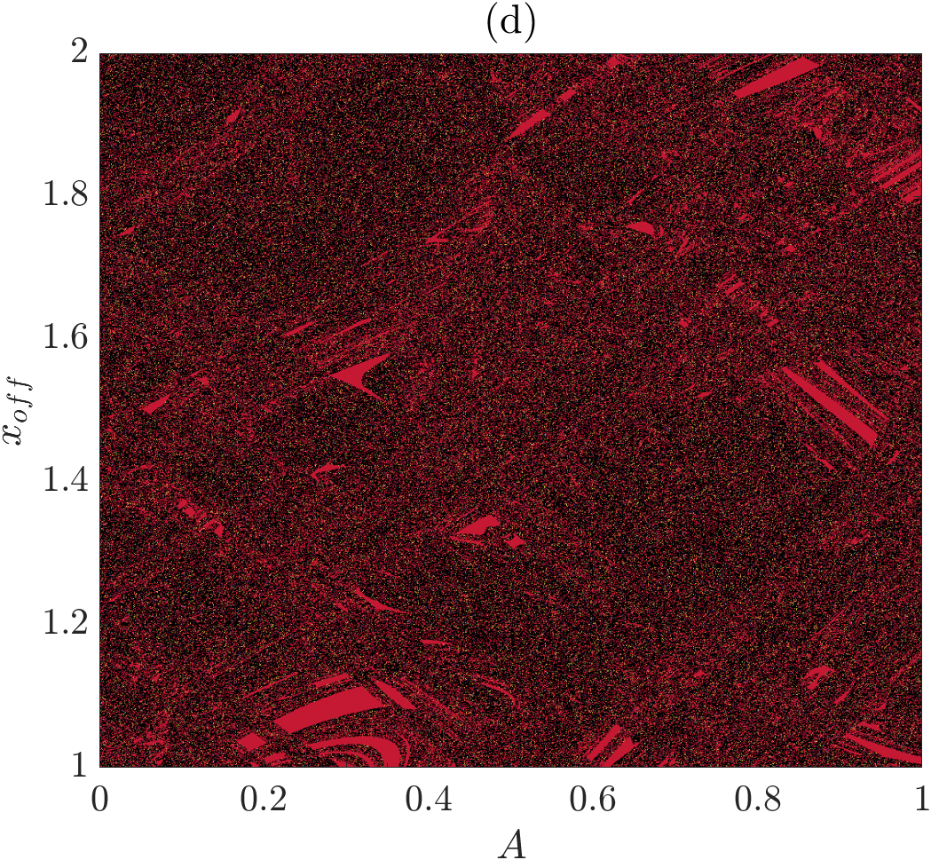
Figure 3: Two-dimensional cross-sections of the state space of the system. Each color corresponds to a different final state of the system when using (4) as initial conditions. Black corresponds to chaotic behavior while color indicates a limit cycle attractor (using the same code as in Fig. 2). Parameters are $(\alpha,\Gamma)=$ $(4,19.5)$ for panel (a), $(4.4,17.2)$ for panel (b), $(4.6,18.2)$ for panel (c) and $(5.9,19.7)$ for panel (d).

V Characterizing multistability: Counting solutions and basin entropy

In order to have a first approach to the way in which the basins of attraction are organized we counted the different coexisting solutions sampling the state space randomly and compared with the calculated the basin entropy using the stochastic method described in Sec. III. Figure 4 display a general overview of the number of attractors (left panels) and the basin entropy (right panels) as a function of the control parameters, $\Gamma$ and $\alpha$. Panels (a) and (c) show the quantity of distinct solutions in the parameter space, sampling initial conditions randomly. To achieve this, we sampled $10^{5}$ initial conditions from a uniform distribution between $0$ and $2$ in contrast to the cross-sectional method explained earlier. For the evolution, we discarded a transient of $1000\Gamma$ and used a $200\Gamma$ long time series to classify the different attractors. We calculated the period, the number of maxima per period and the ordering of those maxima for each time series to characterize and distinguish each attractor.

As we can see in Fig. 4(a) and (c) the system is highly multistable, exhibiting from only one up to 16 coexisting solutions in some of the regions explored. This fact raises the question about the nature of the corresponding basins of attraction for each solution and the characteristics of the interface that separates them. To answer these questions Fig. 4(b) and (d) show the corresponding basin entropy of each region calculated using the method described in section III. The basin entropy also reveals interesting dynamics in Fig 4(b) and (d), in both panels there appears to be a curve where the basin entropy exhibits a local maxima. In the next Section we will show that this curve is near the extinction of the limit-cycle solutions or at least the dominance of the chaotic attractor (see Fig. 5). This behavior of the basin entropy indicates that the structure of the basins of attraction becomes very intricate close to this curve and could the indicator of a bifurcation Daza, Wagemakers, and Sanjuán (2023); Tarigo et al. (2024).

Figure 4 also demonstrates that basin entropy does not necessarily correlate with a large number of coexisting attractors. For instance, the bottom right corner of Fig. 4(c) exhibits the highest number of coexisting attractors, yet the entropy in that region is nearly zero. The points in Fig. 4(d) correspond to the cross sections in Fig. 3. To explore this further, in the next Section we measure the evolution of the basin fraction for each attractor as the parameters were varied along the dashed lines shown in Fig. 4(b) and (d).

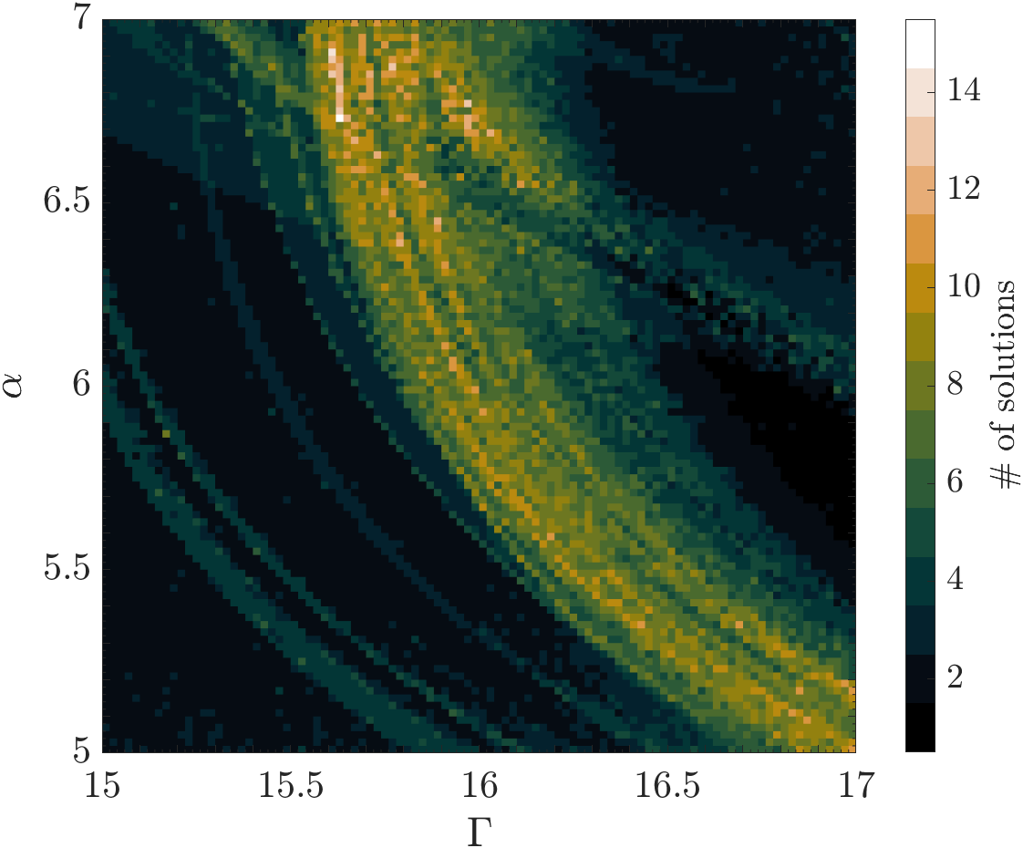
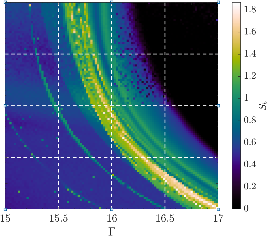
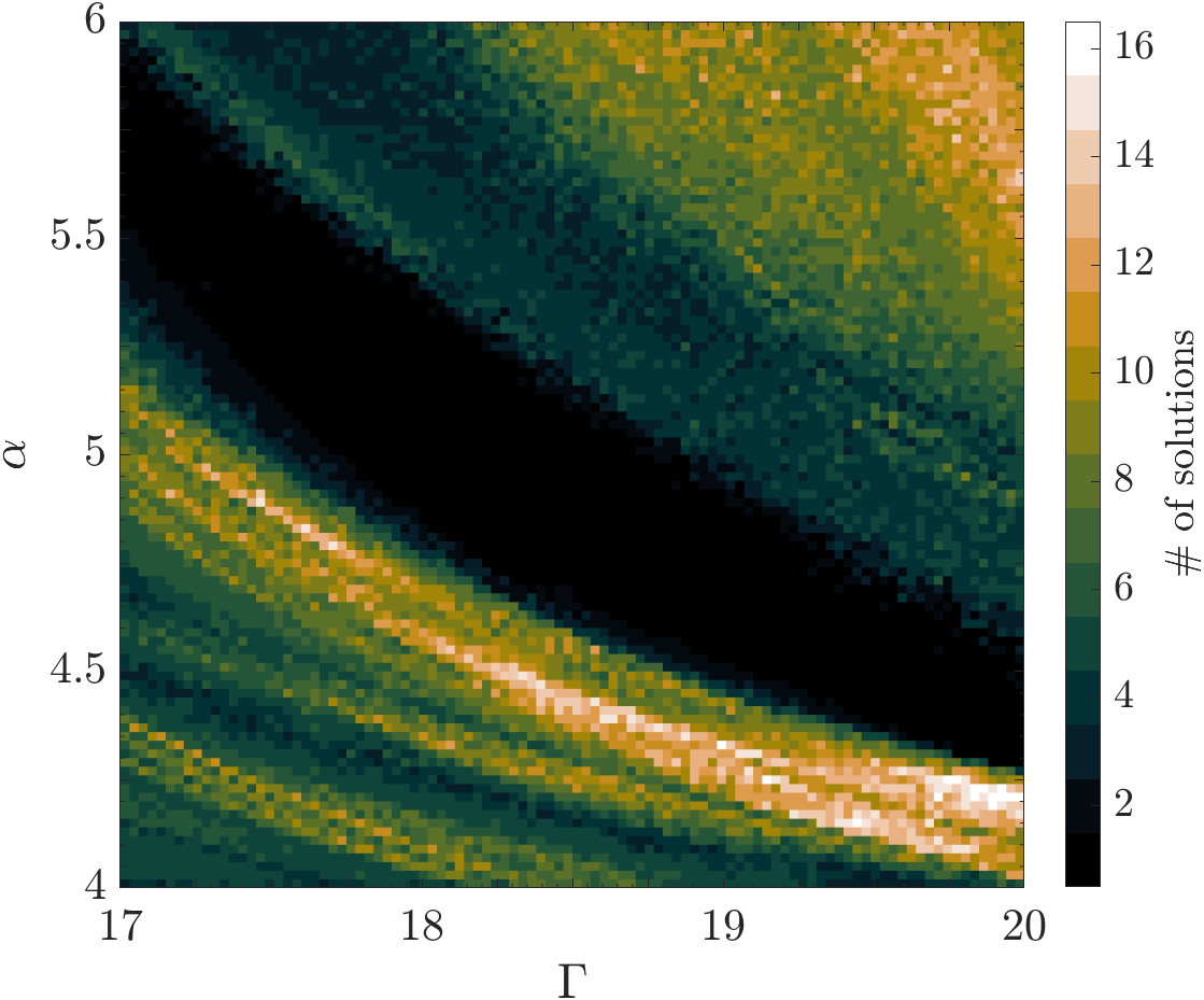
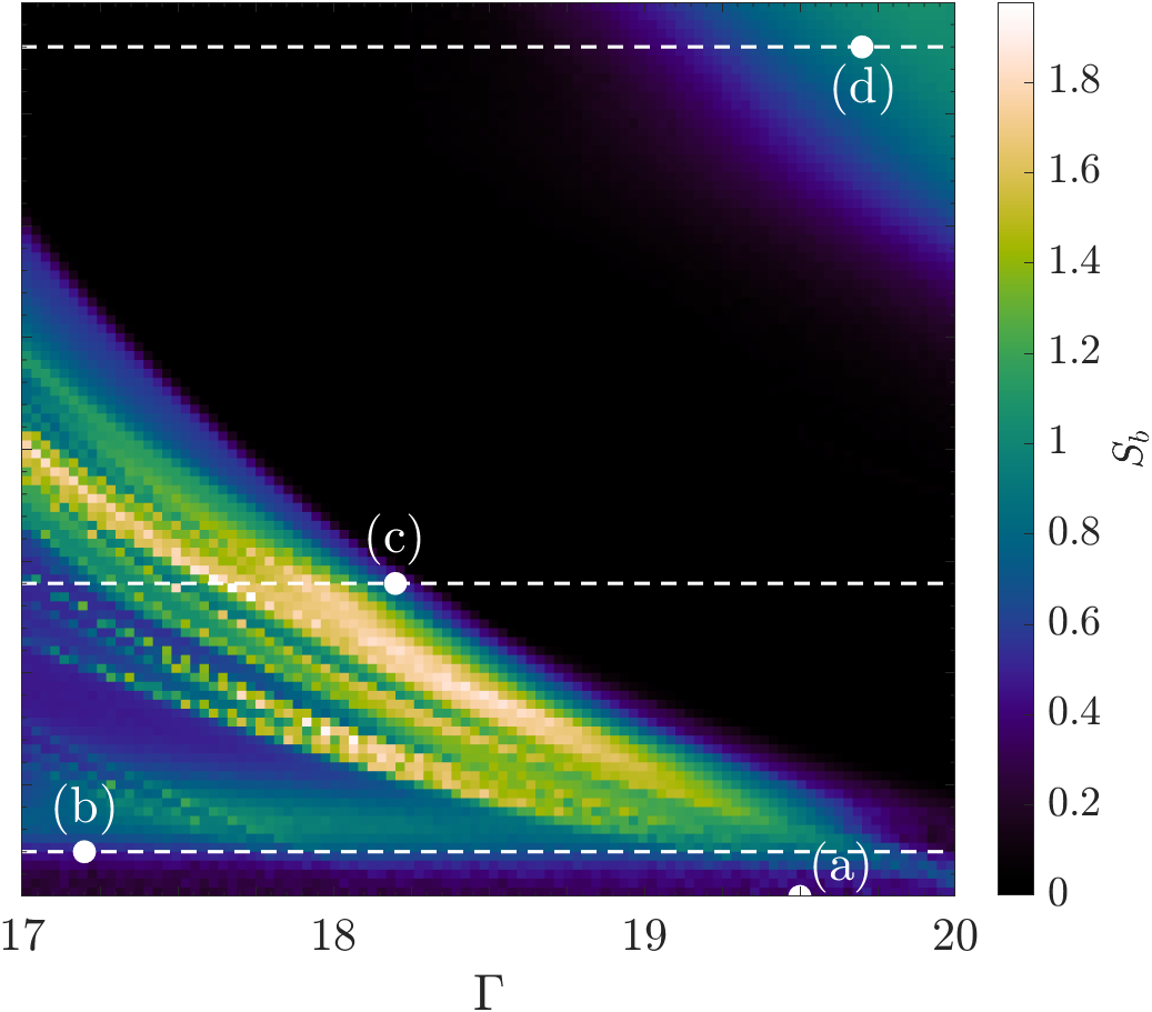
Figure 4: Multistability in the parameter space of the system. Panels (a) and (c) show the number of distinct attractors for each point in the parameter space while panels (b) and (d) show its corresponding basin entropy. For each point in the parameter space $10^{5}$ initial conditions were sampled randomly from a uniform distribution between $0$ and $2$ evenly distributed between $100$ boxes. Then, solutions were matched through its period, its number of maxima per period and the ordering of those maxima in order to obtain the number of different attractors. White points correspond to the cross-sections in Fig. 3 while dashed lines correspond to the diagrams of Fig. 5.

VI Relationship between basin entropy and basin fraction

To better understand the structure of basins of attraction in Fig. 5, we jointly show the fraction of basins and the entropy of basins along sections of parameter space of constant $\Gamma$ or $\alpha$. We can observe that as the parameters change, different attractors emerge and others disappear and their basin fraction and basin entropy also varies. We can also notice that changes in the basin entropy do not necessarily correlate with changes in the basin fraction. The reason for that is that even though the basins of attraction may occupy a larger or smaller fraction their basin boundaries may or may not become more or less riddled.

Figure 5(d) reveals why the basin entropy is low in the bottom right corner of Fig 4(d) even though there is very high number of coexisting attractors in the bottom right corner of Fig. 4(c). Most attractors in this region of the parameters space have very low basin fraction compared to the strange attractor meaning they occupy a small region of the state space and thus their contribution to the basin entropy is negligible. So even though there is a very high attractor count in this region the strange attractor dominates the state space rendering basin entropy almost zero.

As we can see in some regions of Fig. 5 the basin entropy remains constant but the attractors measured change (different colors in the basin fraction diagrams) even though there is no change in the basin fraction. In other instances there is a spike in basin entropy where the attractor becomes a new one. The fact that basin entropy and basin fraction remain constant even when changing attractor is an indication of an immutability of the basins of attraction in those regions even though the attractors themselves are experiencing some mutations. Moreover, the spikes in the basin entropy indicate that for those parameters not only the attractors mutate but their basins of attraction get more intermixed. This results could be hinting at bifurcations in the system and could be further studied using attractor continuation as in Ref. Datseris, Luiz Rossi, and Wagemakers, 2023 to assess if the difference when the basin entropy remains constant are just continuations of the old ones or if they are actually new attractors.

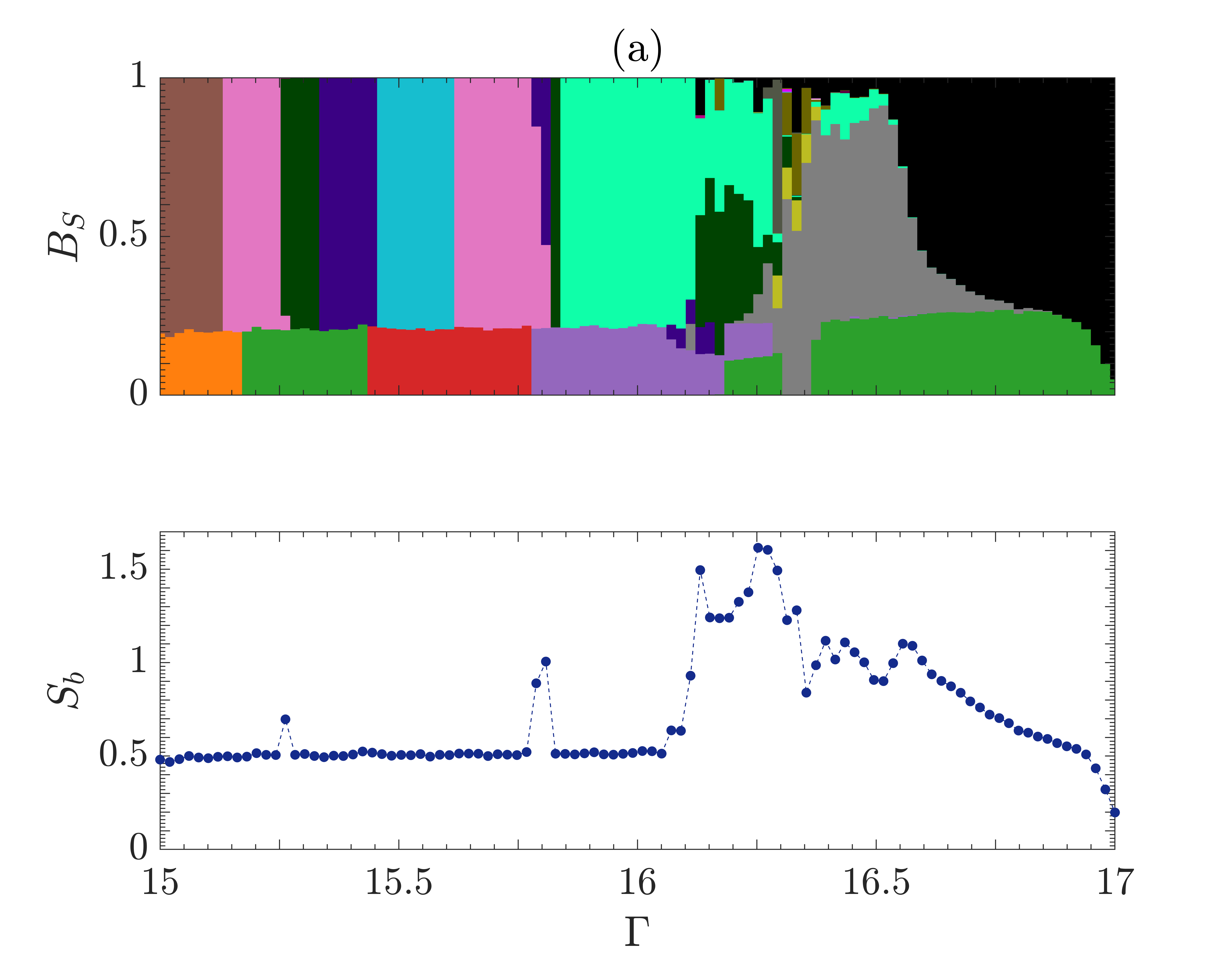
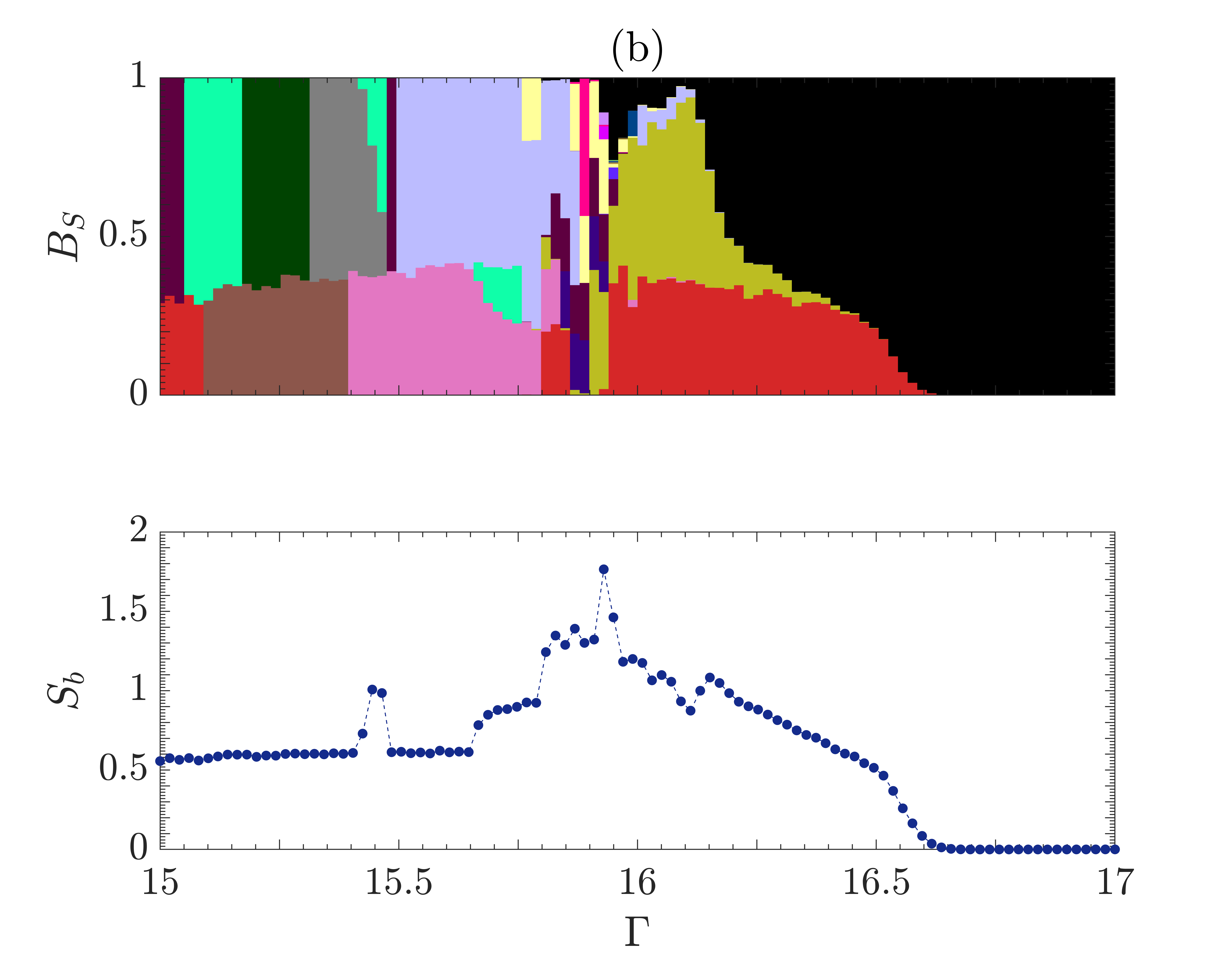
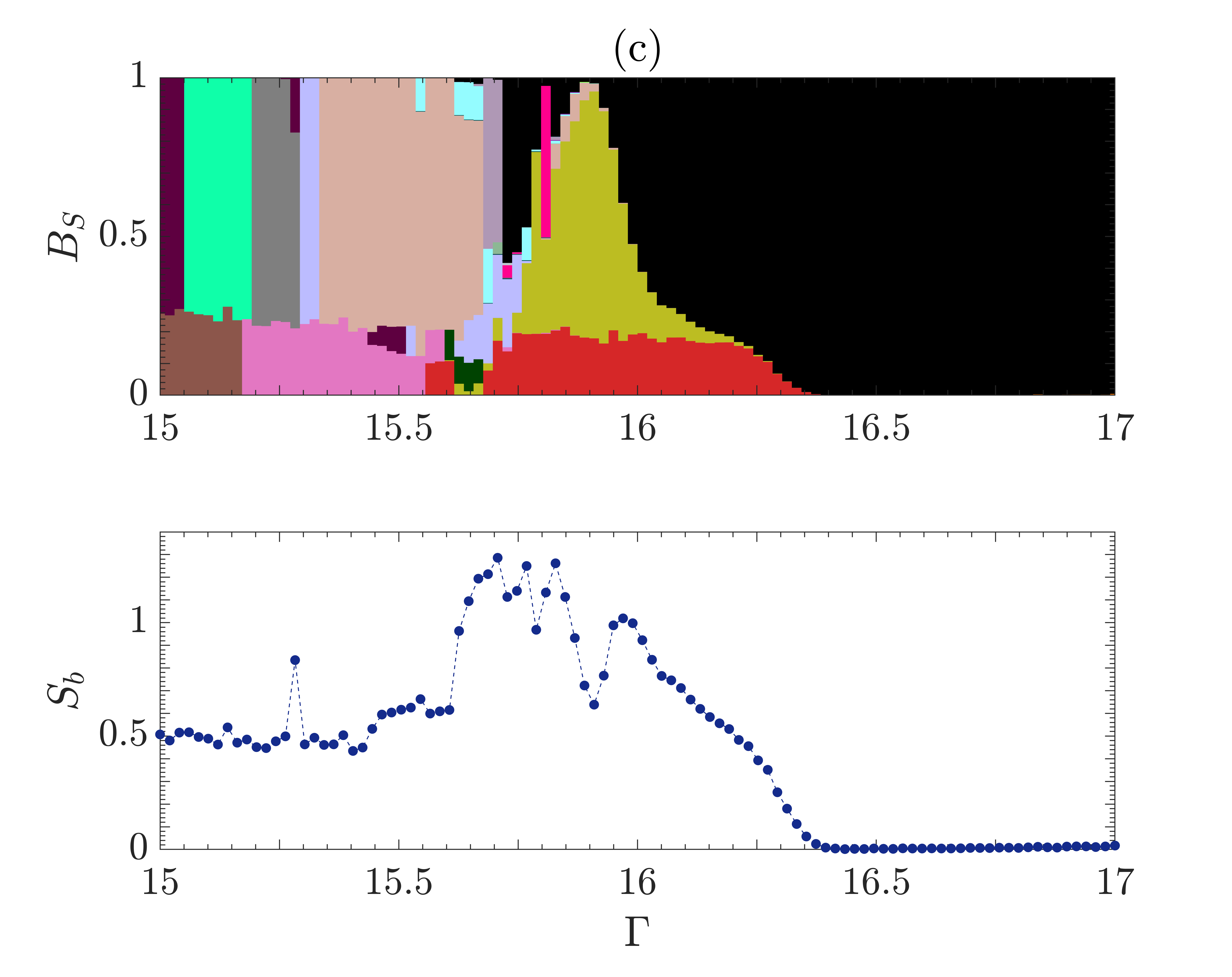
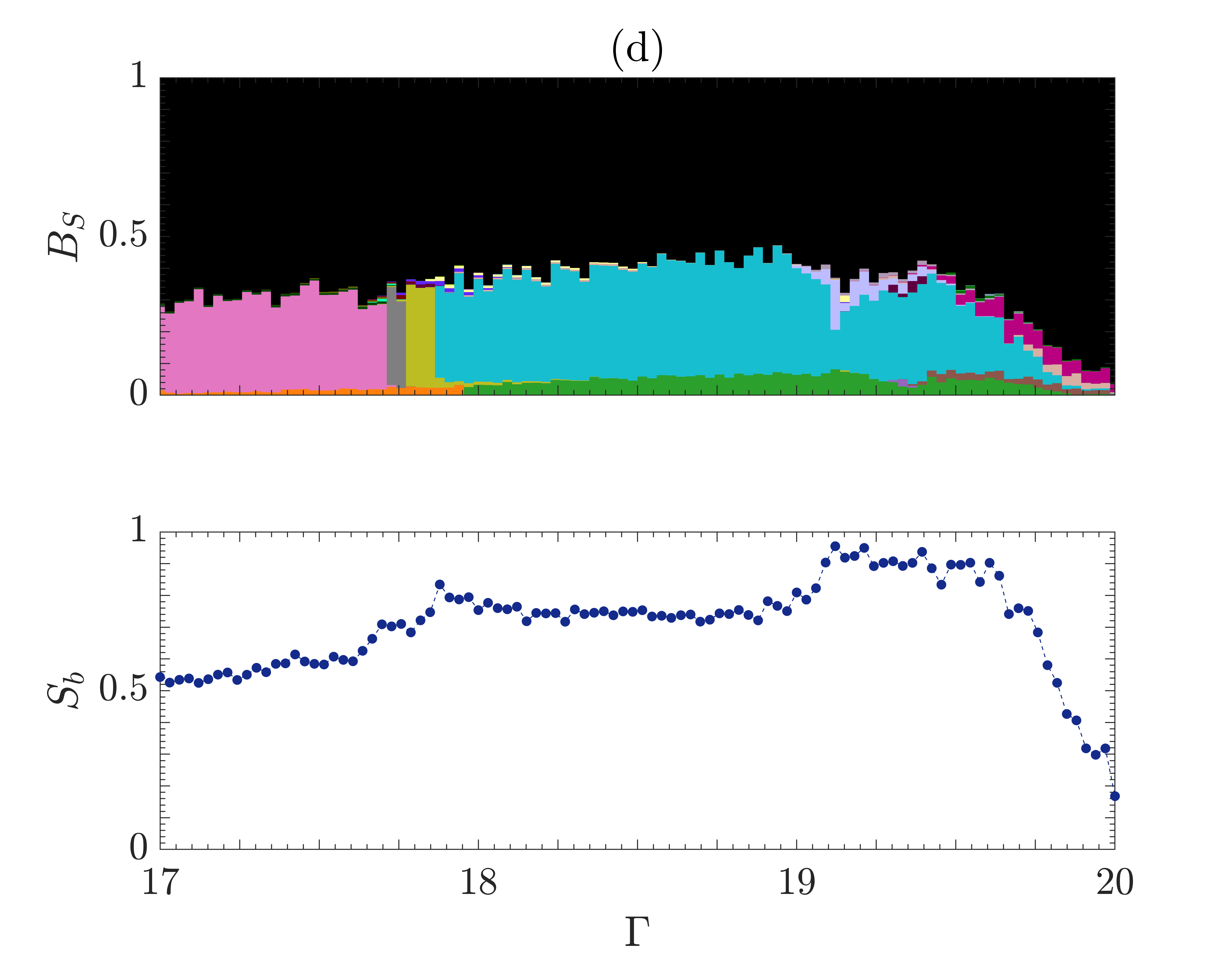
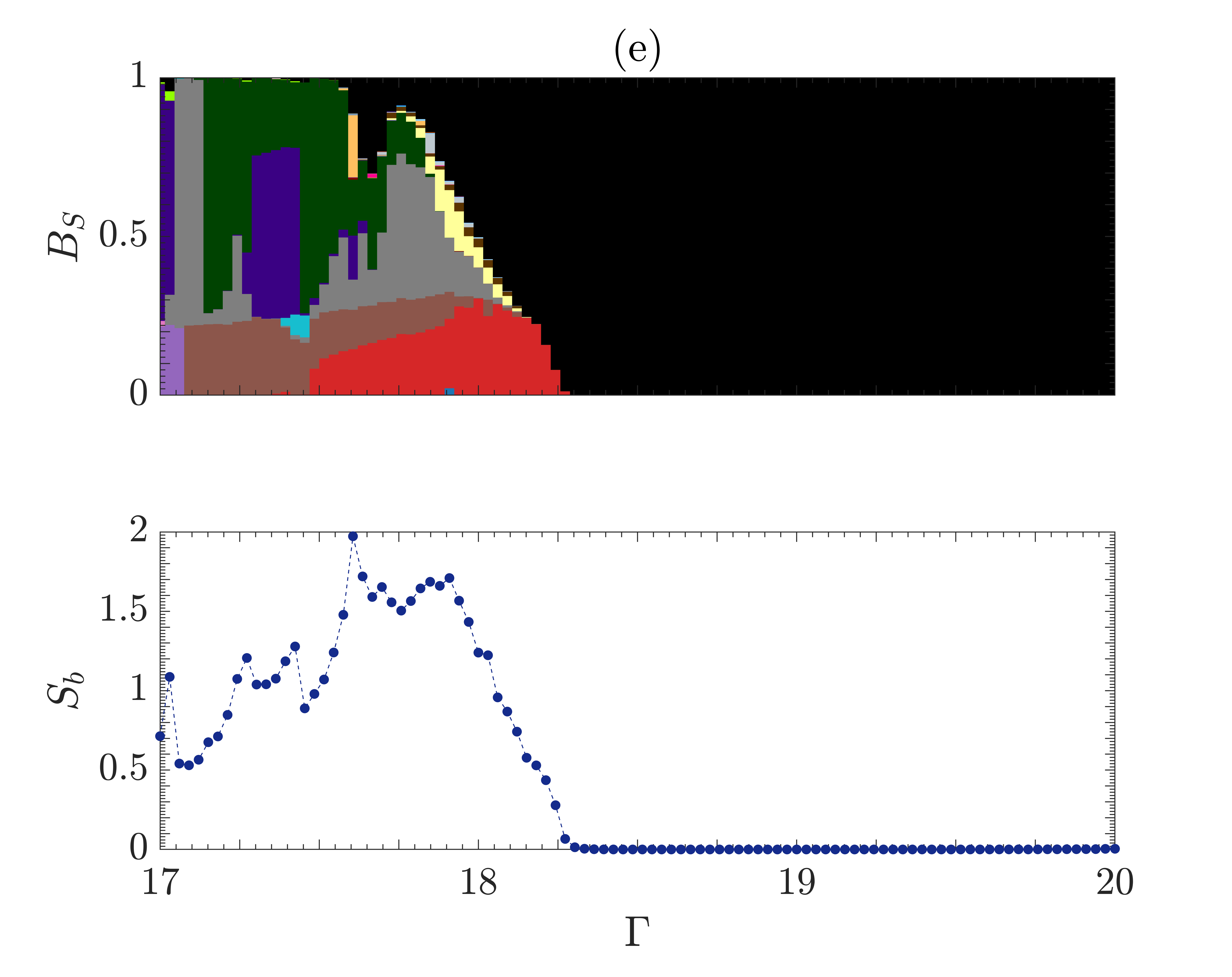
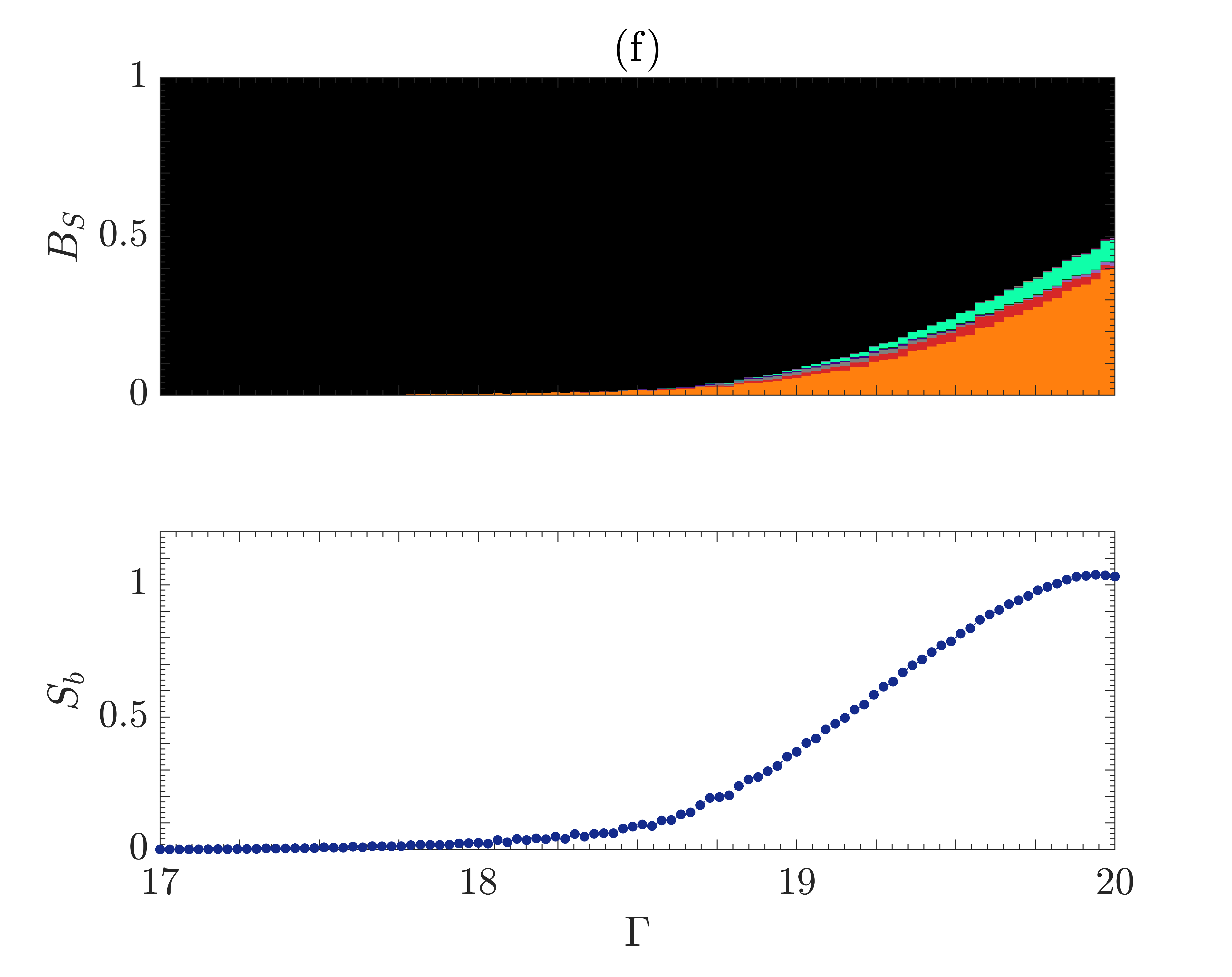
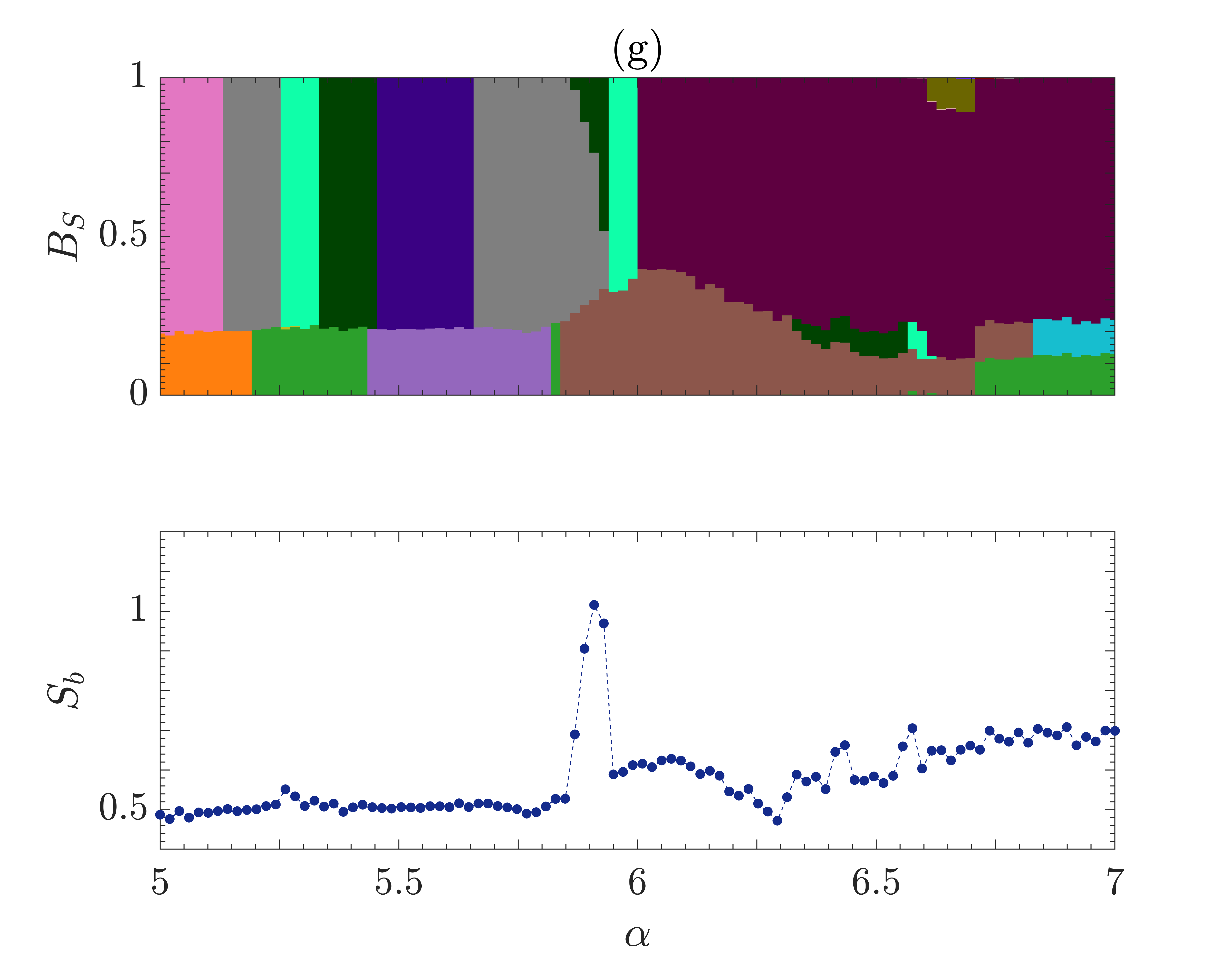
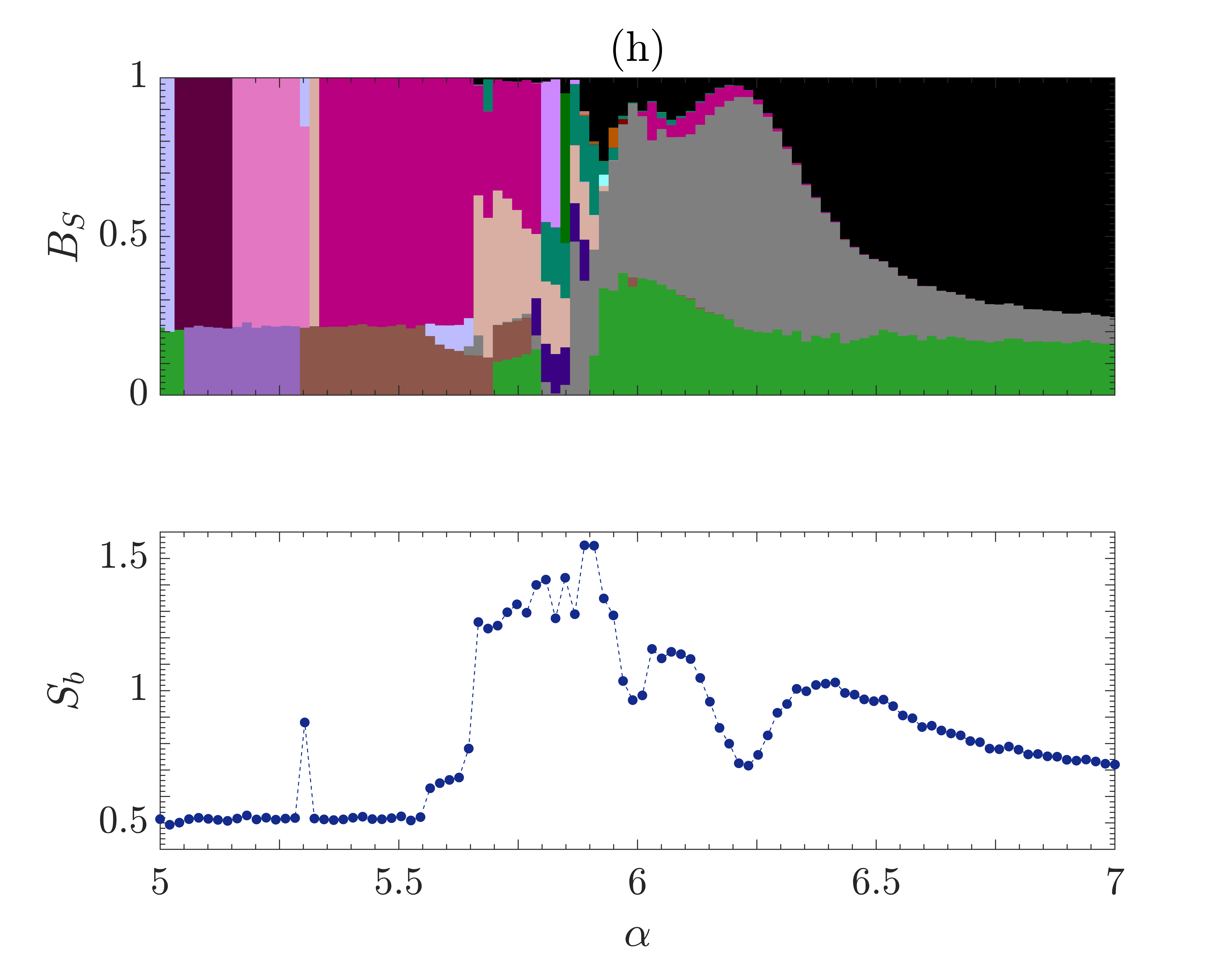
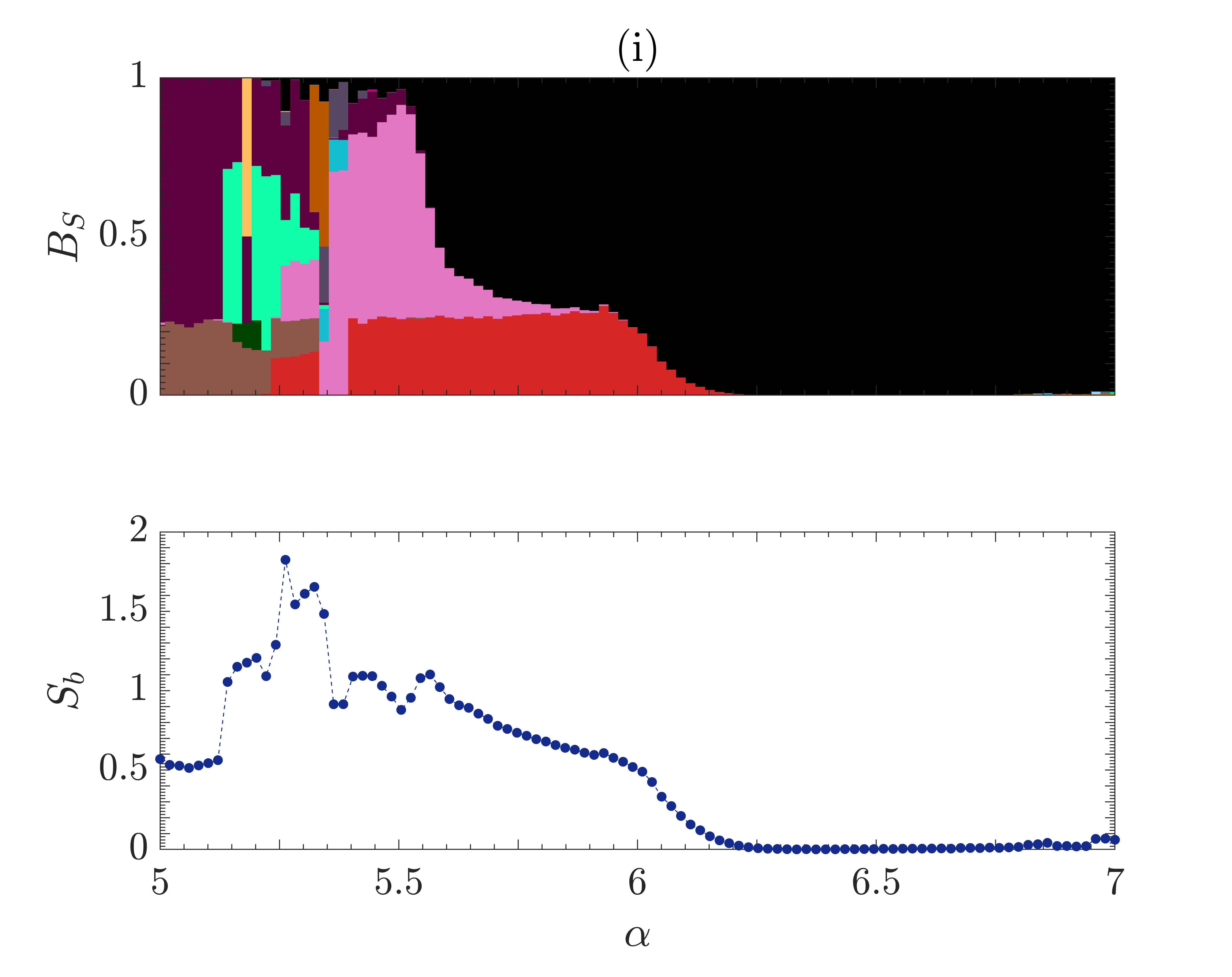
Figure 5: Basin fraction (top) and basin entropy (bottom) for 9 lines in the parameter space. Black corresponds to chaotic behavior while color indicates a limit cycle attractor. (a), (b) and (c) correspond to $\Gamma\in[15,17]$ and $\alpha=5.5$, $\alpha=6$ and $\alpha=6.5$ respectively, (d), (e) and (f) correspond to $\Gamma\in[17,20]$ and $\alpha=4.1$, $\alpha=4.7$ and $\alpha=5.9$ respectively and (g), (h) and (i) correspond to $\alpha\in[5,7]$ and $\Gamma=15.5$, $\Gamma=16$ and $\Gamma=16.5$ respectively.

VII Conclusions

In this work, we investigated the structure of the infinite-dimensional initial condition space of the Mackey-Glass system using complementary techniques. We generalized the concept of basin entropy by randomly sampling the points where we centered the boxes defining set of initial conditions and showed that this method converges rapidly to the basin entropy calculated taking regular lattices. This generalization allowed us to obtain representative samples of the infinite-dimensional space and gain a global understanding of how the basins of attraction are distributed. This method was complemented by counting the number of distinct basins and determining the fraction of volume occupied by each one.

We tested this new method in a discretization of the Mackey-Glass delayed model previously validated with experimental results and numerical methods. and found that, combined with the basin fraction, it can help to understand the composition of the basins of attraction in the state state of high-dimensional systems. We also found that the unpredictability of the system due to its multistability is not only determined by the number of distinct coexisting attractors but also by the relative volume of their corresponding basins of attraction and the morphology of their basin boundaries. Using the basin entropy and basin fraction methods we were able to study these characteristics of the system and give quantitative results of its predictability which would be difficult otherwise due to the high-dimensionality of the system. We also found that this discretization of the Mackey-Glass model presents a maximum of entropy near the extinction of the limit-cycle solutions, hinting at a bifurcation in the system. The application of these techniques to other high-dimensional dynamical systems could provide deeper insights into their multistability and predictability, potentially unveiling new connections between basin structure, system behavior, and underlying bifurcations.