On-the-Fly Ab Initio Hagedorn Wavepacket Dynamics: Single Vibronic Level Fluorescence Spectra of Difluorocarbene
Abstract
Hagedorn wavepackets have been used with local harmonic approximation to partially capture the anharmonic effects on single vibronic level (SVL) spectra in model potentials. To make the Hagedorn approach practical for realistic anharmonic polyatomic molecules, here we combine local harmonic Hagedorn wavepacket dynamics with on-the-fly ab initio dynamics. We then test this method by computing the SVL fluorescence spectra of difluorocarbene, a small, floppy molecule with a very anharmonic potential energy surface. Our time-dependent approach obtains the emission spectra of all initial vibrational levels from a single anharmonic semiclassical wavepacket trajectory without the need to fit individual anharmonic vibrational wavefunctions and to calculate the Franck–Condon factors for all vibronic transitions. We show that, whereas global harmonic models are inadequate for CF2, the spectra computed with the on-the-fly local harmonic Hagedorn wavepacket dynamics agree well with experimental data, especially for low initial excitations.
In the single vibronic level (SVL) fluorescence experiment, a molecule is first excited by a precise light source to a specific vibrational level in the electronic excited state, and its emission from that level is then measured. This emission spectrum provides information on the excited-state relaxation processes and on the higher vibrational levels of the ground electronic state [1, 2, 3, 4, 5, 6].
Following Tapavicza’s generating function approach [7] and our derivation of algebraic expressions for the overlaps between any two Hagedorn functions [8], we recently developed a simple, time-dependent method for computing SVL spectra with Hagedorn wavepacket dynamics [9, 10, 11]. In this method, instead of individually evaluating the Franck–Condon overlaps for all vibronic transitions, the final spectrum is computed from the autocorrelation function between the initial wavepacket and the wavepacket propagated on the final electronic surface. This approach avoids the need to preselect the relevant transitions and can account for mode-mixing (Duschinsky rotation) and anharmonic effects more efficiently, avoiding the calculations of peaks that are not resolved in the experimental spectra. In addition, the Hagedorn approach has the advantage that a single Gaussian wavepacket trajectory is sufficient to compute the SVL emission spectra from any initial vibronic level.
Our approach was validated in harmonic model potentials [9], where the Hagedorn wavepackets are exact solutions to the time-dependent Schrödinger equation, and it was successfully applied to anthracene using a global harmonic model constructed from density functional theory calculations [10]. To investigate whether the Hagedorn method can capture moderate anharmonicity, we combined it with the local harmonic approximation (LHA) and, in a proof-of-principle study, demonstrated an improvement over global harmonic models in Morse systems for which exact quantum calculations were possible [11].
To make the method practical for real polyatomic molecules, here we build on these preliminary results by combining the local harmonic Hagedorn wavepacket approach with on-the-fly ab initio semiclassical [12] dynamics [13, 14, 15, 16, 17, 18, 19]. Similar to the thawed Gaussian approximation [20, 21] used to evaluate ground-level emission and absorption spectra [22, 23, 24, 25, 26], the trajectory-based Hagedorn wavepacket dynamics avoids the need for a full precomputed anharmonic potential energy surface and instead relies on potential energy information evaluated locally during propagation. To test the on-the-fly Hagedorn approach in a realistic system, we compute the SVL spectra of difluorocarbene (CF2), for which experimental results are available from the ground level up to the sixth excitation in the bending mode [27]. By extending the LHA to Hagedorn wavepacket dynamics, we aim to compute the emission from higher vibrational levels and simultaneously include the anharmonic effects without the need for variational or perturbative correction schemes.
In the Hagedorn wavepacket approach to SVL spectroscopy [9], the initial state with vibrational quantum numbers in the electronic excited state is represented in the excited-state normal-mode coordinates by the Hagedorn function [28, 29],
| (1) |
constructed from a -dimensional, normalized, complex-valued Gaussian wavepacket (representing the ground vibrational wavefunction),
| (2) |
by applying the Hagedorn raising operator [30, 31],
| (3) |
In Eq. (1), , and , where is the -th component of the raising operator . In Eq. (2), is the shifted position, and the Gaussian wavepacket is parametrized by its “classical” position and momentum , two complex-valued -dimensional matrices and (such that is the complex symmetric width matrix), and the classical action . Matrices and , related to the position and momentum covariances of the Gaussian [32], satisfy the symplecticity conditions [33, 31],
| (4) | ||||
| (5) |
This parametrization, originally proposed by Hagedorn [34, 35], facilitates the construction of Hagedorn functions (1) from Eqs. (2) and (3). These functions have the form of a Gaussian multiplied by polynomial [30, 31] and are related to the generalized coherent states [36, 37, 38, 39, 40].
By propagating the initial vibrational wavepacket on the electronic ground-state surface , we obtain the autocorrelation function
| (6) |
whose Fourier transform [41, 42, 7]
| (7) |
gives the rate of spontaneous emission from the vibrational level in the excited electronic state to the ground electronic state as a function of frequency . In Eqs. (6) and (7), is the ground-state Hamiltonian, is the (constant) transition dipole moment within the Condon approximation, and is the vibronic energy of the initial state.
In the local harmonic approximation, the ground-state potential is expanded at each time around the current center of the wavepacket as
| (8) |
Remarkably, Hagedorn wavepackets remain exact solutions to the time-dependent Schrödinger equation under this local harmonic potential , with a set of particularly simple, classical-like equations,
| (9) | ||||||
where is the mass matrix and is the Lagrangian [33, 35, 31, 32]. These equations of motion are identical to those in the thawed Gaussian approximation, and the local harmonic propagation of the Hagedorn functions depends simply on the evolution of the Gaussian. Therefore, the SVL spectra from all vibrational levels may be computed “for free” from the same trajectory of the five parameters , needed already to evaluate the ground-level emission. The overlaps between the two Hagedorn wavepackets in the autocorrelation function (6) can be computed from the recurrence relations derived in Ref. 8. The cost of these overlaps is negligible compared with the cost of ab initio calculations required to propagate the guiding Gaussian.
We assume that the initial wavepacket is a vibrationally excited state of a harmonic potential, which can be represented either by a single Hagedorn function (1) with a diagonal matrix or, equivalently, by the product
| (10) |
of a Gaussian and univariate Hermite polynomials [31, 9]. Here, we used the mass-weighted normal-mode coordinates of the initial, excited electronic surface, and is the angular frequency of the -th vibrational mode with a common mass . In general, however, Hagedorn functions are not simple products of one-dimensional Hermite functions [38, 43]. Under the effect of Duschinsky rotation, the excited-state vibrational eigenfunction will not remain separable if it is propagated with the ground-state potential. Yet, with the local harmonic Hagedorn wavepacket dynamics, the multi-index of each Hagedorn function remains constant during the propagation of the parameters of the associated Gaussian.
To assess the accuracy of the local harmonic Hagedorn wavepacket dynamics in a realistic system, we computed the emission spectra from the vibrational ground () level and the first six excited vibrational levels ( to ) in the bending mode () of difluorocarbene (CF2) and compared them to the experiments [27].
Difluorocarbene is an important intermediate in organic synthesis and is used to incorporate fluorocarbon units into medicinal and agricultural compounds [44, 45, 46]. This radical is also generated during the fluorocarbon plasma etching process [47, 48, 49] and during the decomposition of chlorofluorocarbons [50, 51], for example, in the atmosphere under sunlight [52, 53]. With only three vibrational degrees of freedom, it also serves as a simple yet realistic model to test methods for simulating spectra beyond the global harmonic approximation.
Chau et al. [54] simulated the SVL spectra of CF2 by fitting the potential energy function in a special form, variationally determining the anharmonic vibrational wavefunctions as a product of one-dimensional harmonic oscillator eigenfunctions, and subsequently iteratively computing the Franck–Condon factors for each transition using the time-independent sum-over-states expression of vibronic spectroscopy.
In our time-dependent method, the local harmonic SVL spectra were evaluated from a single anharmonic on-the-fly wavepacket trajectory, obtained by evaluating the potential energy , gradient , and Hessian locally at each time step and propagating the wavepacket according to Eqs. (9). All electronic structure calculations were performed with Gaussian 16 [55] at the PBE0/aug-cc-pVTZ level of theory [56, 57]. See the Supplemental Material for the optimized geometries and frequencies of CF2 in the ground and first excited singlet states compared to the experimental data.
To investigate the importance of anharmonicity, we simulated the and spectra also using Hagedorn dynamics combined with one of two global harmonic approximations [9, 10]. The adiabatic harmonic model employs the expansion
| (11) |
of the potential around the optimized ground-state equilibrium geometry , whereas the vertical harmonic model employs the expansion
| (12) |
of the potential around the Franck–Condon point, that is, the optimized excited-state equilibrium geometry .
In both the local and global harmonic simulations, the parameters of the Gaussian were propagated for a total time of (387 fs) with a time step of 8 a.u. The autocorrelation functions between the Hagedorn wavepackets were computed every two steps for each initial vibrational level using the algebraic algorithm from Ref. 8. A Gaussian damping function was applied to the autocorrelation functions such that the spectral peaks were broadened by a Gaussian with a half-width at half-maximum of .
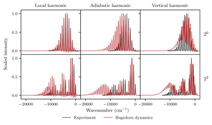
Figure 1 compares the emission spectra from vibrational levels and computed using the local and global harmonic models with the experimental spectra. To facilitate the comparison, we scaled both the computed and experimental spectra by setting the intensity of the highest peak in each spectrum to unity and shifted the wavenumbers of all spectra such that the transition to the vibrational ground level was at .
In the ground-level spectrum (, first row), the adiabatic harmonic model describes the higher-frequency peaks reasonably well and provides the correct spacing between the peaks. However, it significantly overestimates the intensity of the peaks in the lower-frequency () region. The vertical harmonic model captures the overall envelope of the spectra quite well but yields a poorly resolved spectrum at lower wavenumbers.
The delocalization of the wavepacket increases with the initial vibrational excitation and amplifies the effects of anharmonicity. Although the adiabatic model qualitatively captures the splitting of the envelope in the spectrum (second row), the splitting positions and the intensity patterns are incorrect. The spectrum of the vertical harmonic model also exhibits splitting of the envelope and arguably captures it better than the adiabatic model, but the resolution remains poor at lower wavenumbers.
In contrast to the global harmonic models, the local harmonic dynamics (first column of Fig. 1) reproduces remarkably well the experimental results both in terms of intensity patterns and peak positions and in both and spectra. Despite overestimating the lower-frequency peaks, the local harmonic spectrum predicts correctly the splitting locations of the envelope. The significant improvement observed with the local harmonic Hagedorn wavepacket dynamics highlights the importance of including anharmonic effects in the SVL spectra of small, floppy molecules, particularly with a higher initial excitation, even when the ground-level spectrum computed with global harmonic models is satisfactory.
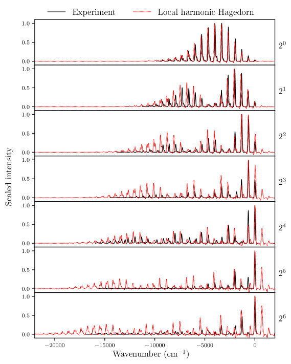
Next, we employed the same on-the-fly ab initio trajectory that we had used for the and spectra to compute the emission spectra also from levels and . To facilitate the comparison of the computed and experimental spectra in Fig. 2, we applied artificial broadening to the experimental values (from Table I in Ref. 27) of the wavelengths and spectral intensities of the emission peaks from to levels.
In Fig. 2, the local harmonic spectra deviate more from the experimental ones as the initial vibrational excitation increases. However, the local harmonic dynamics still captures the correct splitting pattern due to the vibrational excitation of the initial state and yields reasonable peak spacing and intensities in higher-frequency regions.
The poorer performance of our approach for spectra with higher initial excitations can be explained by the more pronounced effects of anharmonicity in both the ground and excited states. On one hand, the wavepacket becomes more delocalized, and the local harmonic trajectory does not fully capture the anharmonicity of the ground-state potential energy surface. On the other hand, the assumption of a harmonic excited-state surface, which justifies representing the initial wavepacket by a single Hagedorn function, may break down as the initial vibrational excitation increases.
Nonetheless, the local harmonic Hagedorn wavepacket approach is suitable for evaluating SVL spectra with relatively low excitations, and its on-the-fly implementation is very efficient. The emission spectra from all vibrational levels are obtained from a single trajectory without the need to rerun expensive electronic structure calculations for different initial states. This advantage becomes even more important in larger systems containing more atoms and electrons.
In conclusion, we successfully combined the local harmonic Hagedorn wavepacket approach with on-the-fly ab initio molecular dynamics to simulate the SVL fluorescence spectra of polyatomic molecules. Using a single semiclassical wavepacket trajectory, we were able to evaluate SVL emission spectra from different initial vibronic levels of the small and flexible CF2 molecule. Whereas the global harmonic models proved to be inadequate for CF2, the local harmonic Hagedorn method resulted in good agreement with the experimental data, at least for lower initial vibrational excitations. Propagation with the local harmonic approximation requires potential energy surface information evaluated only at a single molecular geometry at each time step, and obtaining SVL emission spectra from arbitrary initial vibrational levels incurs minimal additional computational expenses with Hagedorn dynamics. Thus, our efficient method can be applied to larger molecules, similar to how the thawed Gaussian approximation has been used for emission and absorption spectra from the ground vibrational level [23, 58, 59]. Finally, the on-the-fly local harmonic Hagedorn wavepacket approach should be applicable to other vibronic spectroscopy techniques involving excited vibrational states [60, 61, 62, 63, 64, 65] and to more situations with non-Gaussian initial states [66, 67], such as the computation of Herzberg–Teller spectra [68, 69, 70, 71] and internal conversion rates [72].
Acknowledgements.
The authors acknowledge financial support from the EPFL.References
- Schlag and v. Weyssenhoff [1969] E. W. Schlag and H. v. Weyssenhoff, J. Chem. Phys. 51, 2508 (1969).
- Parmenter and Schuyler [1970] C. Parmenter and M. Schuyler, in Transitions non radiatives dans les molécules : 20e réunion de la Société de chimie physique, Paris, 27 au 30 mai 1969 (Société de chimie physique, 1970) p. 92.
- Felker and Zewail [1985] P. M. Felker and A. H. Zewail, J. Chem. Phys. 82, 2975 (1985).
- Quack and Stockburger [1972] M. Quack and M. Stockburger, J. Mol. Spec. 43, 87 (1972).
- Smith et al. [2022] T. C. Smith, M. Gharaibeh, and D. J. Clouthier, J. Chem. Phys. 157, 204306 (2022).
- Suzuki et al. [2024] R. Suzuki, K. Chiba, S. Tanaka, and K. Okuyama, J. Chem. Phys. 160, 024301 (2024).
- Tapavicza [2019] E. Tapavicza, J. Phys. Chem. Lett. 10, 6003 (2019).
- Vaníček and Zhang [2024] J. J. L. Vaníček and Z. T. Zhang, On Hagedorn wavepackets associated with different Gaussians (2024), arXiv:2405.07880 [quant-ph].
- Zhang and Vaníček [ress] Z. T. Zhang and J. J. L. Vaníček, J. Chem. Phys. doi:10.1063/5.0219005 (in press), arXiv:2403.00577 [physics.chem-ph].
- Zhang and Vaníček [2024] Z. T. Zhang and J. J. L. Vaníček, Ab initio simulation of single vibronic level fluorescence spectra of anthracene using Hagedorn wavepackets (2024), arXiv:2403.00702 [physics.chem-ph].
- Zhang et al. [2024] Z. T. Zhang, M. Visegrádi, and J. J. L. Vaníček, Capturing anharmonic effects in single vibronic level fluorescence spectra using local harmonic Hagedorn wavepacket dynamics (2024), arXiv:2408.11991 [physics.chem-ph].
- Miller [2001] W. H. Miller, J. Phys. Chem. A 105, 2942 (2001).
- Tatchen and Pollak [2009] J. Tatchen and E. Pollak, J. Chem. Phys. 130, 041103 (2009).
- Ceotto et al. [2009] M. Ceotto, S. Atahan, S. Shim, G. F. Tantardini, and A. Aspuru-Guzik, Phys. Chem. Chem. Phys. 11, 3861 (2009).
- Wong et al. [2011] S. Y. Y. Wong, D. M. Benoit, M. Lewerenz, A. Brown, and P.-N. Roy, J. Chem. Phys. 134, 094110 (2011).
- Saita and Shalashilin [2012] K. Saita and D. V. Shalashilin, J. Chem. Phys. 137, 22A506 (2012).
- Ceotto et al. [2017] M. Ceotto, G. Di Liberto, and R. Conte, Phys. Rev. Lett. 119, 010401 (2017).
- Di Liberto et al. [2018] G. Di Liberto, R. Conte, and M. Ceotto, J. Chem. Phys. 148, 104302 (2018).
- Pios et al. [2024] S. V. Pios, M. F. Gelin, L. Vasquez, J. Hauer, and L. Chen, J. Phys. Chem. Lett. 15, 8728 (2024).
- Heller [1975] E. J. Heller, J. Chem. Phys. 62, 1544 (1975).
- Heller [2018] E. J. Heller, The Semiclassical Way to Dynamics and Spectroscopy (Princeton University Press, Princeton, NJ, 2018).
- Wehrle et al. [2014] M. Wehrle, M. Šulc, and J. Vaníček, J. Chem. Phys. 140, 244114 (2014).
- Wehrle et al. [2015] M. Wehrle, S. Oberli, and J. Vaníček, J. Phys. Chem. A 119, 5685 (2015).
- Begušić et al. [2022] T. Begušić, E. Tapavicza, and J. Vaníček, J. Chem. Theory Comput. 18, 3065 (2022).
- Klētnieks et al. [2023] E. Klētnieks, Y. C. Alonso, and J. J. L. Vaníček, J. Phys. Chem. A 127, 8117 (2023).
- Gherib et al. [2024] R. Gherib, I. G. Ryabinkin, and S. N. Genin, Thawed Gaussian wavepacket dynamics with -machine learned potentials (2024), arXiv:2405.00193 [physics.chem-ph].
- King et al. [1979] D. S. King, P. K. Schenck, and J. C. Stephenson, J. Mol. Spec. 78, 1 (1979).
- Hagedorn [1981] G. A. Hagedorn, Ann. Phys. (NY) 135, 58 (1981).
- Hagedorn [1985] G. A. Hagedorn, Ann. Henri Poincaré 42, 363 (1985).
- Hagedorn [1998] G. A. Hagedorn, Ann. Phys. (NY) 269, 77 (1998).
- Lasser and Lubich [2020] C. Lasser and C. Lubich, Acta Numerica 29, 229 (2020).
- Vaníček [2023] J. J. L. Vaníček, J. Chem. Phys. 159, 014114 (2023).
- Lubich [2008] C. Lubich, From Quantum to Classical Molecular Dynamics: Reduced Models and Numerical Analysis (European Mathematical Society, Zürich, 2008).
- Hagedorn [1980] G. A. Hagedorn, Commun. Math. Phys. 71, 77 (1980).
- Faou et al. [2009] E. Faou, V. Gradinaru, and C. Lubich, SIAM J. Sci. Comp. 31, 3027 (2009).
- Combescure [1992] M. Combescure, J. Math. Phys. 33, 3870 (1992).
- Combescure and Robert [2012] M. Combescure and D. Robert, Coherent States and Applications in Mathematical Physics, Theoretical and Mathematical Physics Ser. (Springer Netherlands, Dordrecht, 2012).
- Lasser and Troppmann [2014] C. Lasser and S. Troppmann, J. Fourier Anal. Appl. 20, 679 (2014).
- Borrelli and Gelin [2016] R. Borrelli and M. F. Gelin, Chem. Phys. 481, 91 (2016).
- Chen et al. [2017] L. Chen, R. Borrelli, and Y. Zhao, J. Phys. Chem. A 121, 8757–8770 (2017).
- Heller [1981] E. J. Heller, Acc. Chem. Res. 14, 368 (1981).
- Tannor [2007] D. J. Tannor, Introduction to Quantum Mechanics: A Time-Dependent Perspective (University Science Books, Sausalito, 2007).
- Ohsawa [2019] T. Ohsawa, J. Fourier Anal. Appl. 25, 1513 (2019).
- Ma et al. [2023] X. Ma, J. Su, and Q. Song, Acc. Chem. Res. 56, 592 (2023).
- Fuchibe and Ichikawa [2023] K. Fuchibe and J. Ichikawa, Chem. Commun. 59, 2532 (2023).
- Xie and Hu [2024] Q. Xie and J. Hu, Acc. Chem. Res. 57, 693 (2024).
- Bulcourt et al. [2004] N. Bulcourt, J.-P. Booth, E. A. Hudson, J. Luque, D. K. W. Mok, E. P. Lee, F.-T. Chau, and J. M. Dyke, J. Chem. Phys. 120, 9499 (2004).
- Lele et al. [2009] C. Lele, Z. Liang, X. Linda, L. Dongxia, C. Hui, and P. Tod, J. Semicond. 30, 033005 (2009).
- Cuddy and Fisher [2012] M. F. Cuddy and E. R. Fisher, ACS Appl. Mater. Interfaces 4, 1733 (2012).
- Fujita et al. [1992] I. Fujita, K. Matsuda, T. Kijima, M. Sakamoto, and M. Hatada, Int. J. Radiat. Appl. Instrum. Part A 43, 641 (1992).
- Sonoyama et al. [2002] N. Sonoyama, K. Ezaki, H. Fujii, and T. Sakata, Electrochim. Acta 47, 3847 (2002).
- Rebbert and Ausloos [1975] R. E. Rebbert and P. J. Ausloos, J. Photochem. 4, 419 (1975).
- Argüello et al. [1994] G. A. Argüello, B. Jülicher, and H. Willner, Angew. Chem. Int. Ed. 33, 1108 (1994).
- Chau et al. [2001] F.-T. Chau, J. M. Dyke, E. P. F. Lee, and D. K. W. Mok, J. Chem. Phys. 115, 5816 (2001).
- Frisch et al. [2016] M. J. Frisch, G. W. Trucks, H. B. Schlegel, G. E. Scuseria, M. A. Robb, J. R. Cheeseman, G. Scalmani, V. Barone, G. A. Petersson, H. Nakatsuji, X. Li, M. Caricato, A. V. Marenich, J. Bloino, B. G. Janesko, R. Gomperts, B. Mennucci, H. P. Hratchian, J. V. Ortiz, A. F. Izmaylov, J. L. Sonnenberg, D. Williams-Young, F. Ding, F. Lipparini, F. Egidi, J. Goings, B. Peng, A. Petrone, T. Henderson, D. Ranasinghe, V. G. Zakrzewski, J. Gao, N. Rega, G. Zheng, W. Liang, M. Hada, M. Ehara, K. Toyota, R. Fukuda, J. Hasegawa, M. Ishida, T. Nakajima, Y. Honda, O. Kitao, H. Nakai, T. Vreven, K. Throssell, J. A. Montgomery, Jr., J. E. Peralta, F. Ogliaro, M. J. Bearpark, J. J. Heyd, E. N. Brothers, K. N. Kudin, V. N. Staroverov, T. A. Keith, R. Kobayashi, J. Normand, K. Raghavachari, A. P. Rendell, J. C. Burant, S. S. Iyengar, J. Tomasi, M. Cossi, J. M. Millam, M. Klene, C. Adamo, R. Cammi, J. W. Ochterski, R. L. Martin, K. Morokuma, O. Farkas, J. B. Foresman, and D. J. Fox, Gaussian 16 Revision C.01 (2016), Gaussian Inc. Wallingford CT.
- Adamo and Barone [1999] C. Adamo and V. Barone, J. Chem. Phys. 110, 6158 (1999).
- Kendall et al. [1992] R. A. Kendall, T. H. Dunning, and R. J. Harrison, J. Chem. Phys. 96, 6796 (1992).
- Begušić et al. [2019] T. Begušić, M. Cordova, and J. Vaníček, J. Chem. Phys. 150, 154117 (2019).
- Begušić and Vaníček [2020] T. Begušić and J. Vaníček, J. Chem. Phys. 153, 024105 (2020).
- van Wilderen et al. [2014] L. J. G. W. van Wilderen, A. T. Messmer, and J. Bredenbeck, Angew. Chem. Int. Ed. 53, 2667 (2014).
- Yu et al. [2014] H. Yu, N. L. Evans, A. S. Chatterley, G. M. Roberts, V. G. Stavros, and S. Ullrich, J. Phys. Chem. A 118, 9438 (2014).
- Baiardi et al. [2014] A. Baiardi, J. Bloino, and V. Barone, J. Chem. Phys. 141, 114108 (2014).
- Whaley-Mayda et al. [2021] L. Whaley-Mayda, A. Guha, S. B. Penwell, and A. Tokmakoff, J. Am. Chem. Soc. 143, 3060 (2021).
- Lau et al. [2023] J. A. Lau, M. DeWitt, M. A. Boyer, M. C. Babin, T. Solomis, M. Grellmann, K. R. Asmis, A. B. McCoy, and D. M. Neumark, J. Phys. Chem. A 127, 3133 (2023).
- Horz et al. [2023] M. Horz, H. M. A. Masood, H. Brunst, J. Cerezo, D. Picconi, H. Vormann, M. S. Niraghatam, L. J. G. W. Van Wilderen, J. Bredenbeck, F. Santoro, and I. Burghardt, J. Chem. Phys. 158, 064201 (2023).
- Lee and Heller [1982] S.-Y. Lee and E. J. Heller, J. Chem. Phys. 76, 3035 (1982).
- Tannor and Heller [1982] D. J. Tannor and E. J. Heller, J. Chem. Phys. 77, 202 (1982).
- Baiardi et al. [2013] A. Baiardi, J. Bloino, and V. Barone, J. Chem. Theory Comput. 9, 4097 (2013).
- Bonfanti et al. [2018] M. Bonfanti, J. Petersen, P. Eisenbrandt, I. Burghardt, and E. Pollak, J. Chem. Theory Comput. 14, 5310 (2018).
- Patoz et al. [2018] A. Patoz, T. Begušić, and J. Vaníček, J. Phys. Chem. Lett. 9, 2367 (2018).
- Kundu et al. [2022] S. Kundu, P. P. Roy, G. R. Fleming, and N. Makri, J. Phys. Chem. B 126, 2899 (2022).
- Wenzel and Mitric [2023] M. Wenzel and R. Mitric, J. Chem. Phys. 158, 034105 (2023).