COOCK project Smart Port 2025 D3.2
“Variability in Twinning Architectures”
Abstract.
This document is a result of the COOCK project “Smart Port 2025: improving and accelerating the operational efficiency of a harbour eco-system through the application of intelligent technologies”. The project is mainly aimed at SMEs, but also at large corporations. Together, they form the value-chain of the harbour. The digital maturity of these actors will be increased by model and data-driven digitization. The project brings together both technology users and providers/integrators. In this report, the broad spectrum of model and data-based digitization approaches is structured, under the unifying umbrella of “Digital Twins”. During the (currently quite ad-hoc) digitization process and in particular, the creations of Digital Twins, a variety of choices have an impact on the ultimately realised system. This document identifies three stages during which this “variability” appears: the Problem Space Goal Construction Stage, the (Conceptual) Architecture Design Stage and the Deployment Stage. To illustrate the workflow, two simple use-cases are used: one of a ship moving in 1 dimension and, at a different scale and level of detail, a macroscopic model of the Port of Antwerp.
1. Introduction
A Digital Twins (DTs) are increasingly seen as a key enabler and backbone for digitization of complex Cyber-Physical Systems (CPSs). The “Twinning Paradigm” combines a System under Study (SuS – also called an Actual Object (AO)) with a corresponding Twin Object (TO), i.e., a model of that system. The Twin Object may be symbolic in nature, or data based.
The concept of “twinning” is not new. Sand tables, for example, have been used since antiquity as “twins” of battlefields, which allowed generals to evaluate and plan troop movements. During the Apollo missions (Ferguson, 2020), NASA used a mirrored training capsule on earth to mimic and, when needed, diagnose anomalies occurring in their deployed spacecraft. While the “twin” is these historical examples is not “digital” (as it exist within physical space), they cover the same twinning concepts as modern-day DTs.
The core idea behind twinning is that the TOs are not just simulation models or data sets, but are continually kept “in sync” with their corresponding AO. The TO is fed the same sensor input as the AO receives. This allows for useful functionality such as “anomaly detection”: significant deviation between AO measurements and TO predictions is an indication that the SuS is not functioning as intended.
Commonly, twins are built to satisfy a specific set of goals pertaining to Properties of Interest (PoIs). These goals are also referred to as the purpose of a twin (Dalibor et al., 2022). An example goal is “anomaly detection”, with for example “energy efficiency” as a Property of Interest. (Qamar and Paredis, 2012) defines a “property” as the “descriptor of an artifact”. Hence, it is a specific concern of that artifact (i.e., a system), which is either logical Some of these properties can be computed (or derived from other, related artifacts), or specified (by a user). Goals consider the specific system PoIs that are of concern to certain stakeholders.
For many products, multiple variants exist. Each of these variants have common parts, aspects, components, …, but varies in others. This is also the case for DTs. For instance, multiple ships of the same type might have different sails, different engines, different control software, …These differences are called features. One may see each variant as a separate configuration of the product. The set of all variants forms a product family. Feature trees/models are often used to describe the elements of a product family.
Figure 1 illustrates a high-level workflow for constructing twinning systems. Firstly, a set of goals (pertaining to PoIs) are identified for which the twin must be created. There can be multiple goals which the twin needs to satisfy. Section 4 goes deeper into this topic.
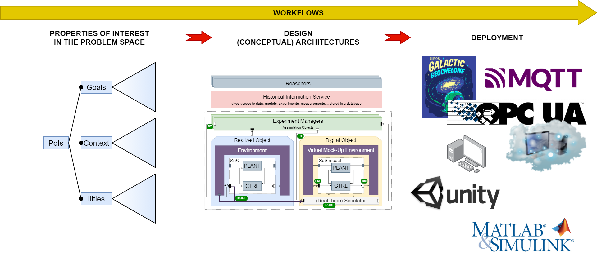
Secondly, based on the chosen goals/PoIs, a conceptual architecture will be chosen. Some components of this a architecture will be present/absent depending on the choices made in the previous stage. The figure illustrates this by including a reference architecture from (Paredis and Vangheluwe, 2022) that has a set of “toggles” or “presence conditions” (i.e., parts that can be enabled/disabled). This is further described in section 5.
Finally, there is the deployment stage in which appropriate technologies are chosen/used to realise this twin. This details the communication protocols, server hardware and operating system, modelling formalism (and toolbox/simulator) etc. Section 6 discusses this topic in more detail.
These three stages are all part of a set of workflows that allows the creation of a twin that implements the desired (and specified) behaviour.
In terms of execution, we will focus on the notion of experiments. An experiment is an intentional set of (hierarchical) activities, carried out on a specific SuS in order to accomplish a specific (set of) goal(s). Each experiment should have a recorded explicit description, setup and workflow, such that becomes is repeatable.
2. Background
Ever since the conceptualization of Digital Twins (DTs) in (Grieves and Vickers, 2017) and its introduction to Industry 4.0 as described in (Boss et al., 2020), a plethora of (reference) architectures have sprouted up. Yet, most of these architectures remain conceptual, or highly abstract to actually translate into a running DT system.
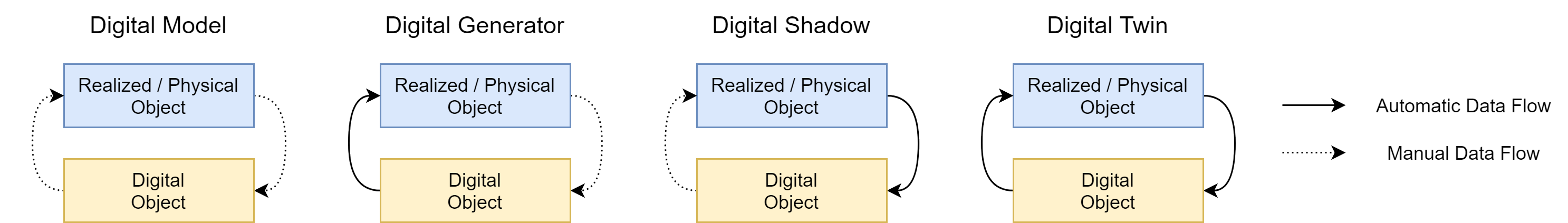
Some architectures focus on the difference in connectivity between the AO and TO. For instance, (Kritzinger et al., 2018) introduces the notion of a Digital Model (DM – when the AO and TO are only connected to each other via a bidirectional manual connection), and a Digital Shadow (DS – when the connection from the AO to the TO is automated). The paper states that a DT only appears if the bidirectional communication has no manual components. (Tekinerdogan and Verdouw, 2020) expands on this notion by introducing a Digital Generator (DG – the dual of the DS, i.e., when the connection from the TO to the AO is automated). This is illustrated in figure 2.
(Tao and Zhang, 2017) leaves the communication aspect be and focuses on the individual parts and components required in a DT. As shown in figure 3, they arrive at the so-called 5D architecture (Van Den Brand et al., 2021), where five components are highlighted: (1) the “Phyiscal Shop-Floor” (i.e., the AO), (2) the “Virtual Shop-Floor” (i.e., the TO), (3) “Shop-Floor Digital Twin Data” (in essence some sort of communication point or data lake), (4) “Shop-Floor Service System (a set of processes that use the data from the AO and the TO – this is commonly called a set of Services), and (5) all the communication between these components.
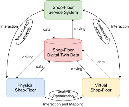
Note that both figures 2 and 3 implicitly incorporate a specific set of design and deployment choices. (Kritzinger et al., 2018) focuses on the communication channel between the AO and the TO. Yet, when considering twinning, this level of communication is the result of a specific design choice of the system, based on which goal and which corresponding PoI it tries to solve, as well as the technologies that are available. (Tao and Zhang, 2017) focuses on a specific domain of a shop-floor, but DTs also exist in a multitude of other domains (Dalibor et al., 2022). Furthermore, the communication point/data lake is clearly already a deployment choice, subtly hinting at OPC-UA like technologies. Additionally, the indication of a “physical” AO and a “virtual” TO already shows a specific choice for the implementation of the DT.
3. Running Examples
We will discuss two running examples to show the presented approach.
3.1. Simple Port Simulation
We present a simplified model of the Port of Antwerp-Bruges (PoAB) in which vessels travel from the North Sea, over the Scheldt river, through canals and locks toward docks, and back. These locks and docks have a finite capacity.
Figure 4 shows a map of the Scheldt through the city of Antwerp. For the sake of simplicity, we highlight the equivalence to road traffic. In the figure, circles indicate junctions where multiple trajectories merge/diverge. The three large squares are the locks and the small diamonds are the docks. The red, dotted lines identify sections of sailing routes on the river. Generally, these are two-way connections, except for the connection from the “loodskotter” source (identified with “K”) and to the sea endpoint (identified with “S”). Canals are represented with full red lines. Next to all river sections and all canals, their distance is denoted.
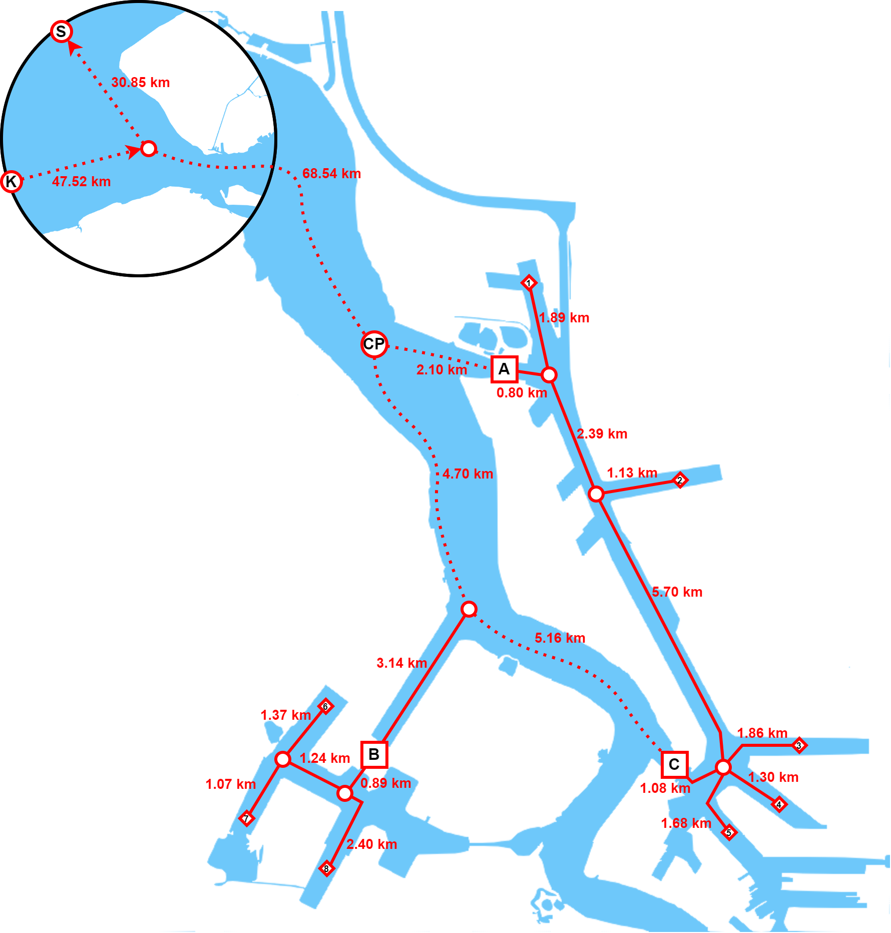
Ships that arrive from “K” are given a target dock to sail to, where they will stay for some time, before departing towards “S”. Each ship type is given its own unique velocity distribution, based on real-world information. The docks can hold at most 50 vessels and the locks are area-constrained (i.e., we will ignore that the top area of a ship is solid). Additionally, ships cannot overtake each other on canals.
The full specification of this PoAB example is found on http://msdl.uantwerpen.be/people/hv/teaching/MoSIS/202223/assignments/DEVS.
This system is clearly an abstraction of the real-world scenario. To make this more interesting and fit within the context of twinning, we will use another simulation of this very same system, with slightly different parameters. This second simulation will be considered the AO and the “source of truth” that we want the TO to conform to.
3.2. 1D Yacht
Another example is a 1-dimensional yacht on water. This is based on an assignment given to Master-level students at the University of Antwerp, thus highlighting the simplicity of this use-case.
Let’s say there exists a yacht that only sails in a single direction (i.e., turning is not incorporated in this example). Furthermore, we will assume that it is not being influenced by sea currents. We would like to construct a Digital Shadow for this yacht, such that we can visualize the differences from the expected behaviour in a simple dashboard. We expect that the yacht follows a specific (repeating) velocity profile (which may be provided by some port authority). This can be modelled using the following Ordinary Differential Equations (ODEs):
Where is the density of sea water (, assuming the temperature is ), is the submerged surface area of the vessel w.r.t. the direction of movement (approximately , based on previous experiments), is the friction value, is Reynolds number, is the length of the yacht (), the dry mass equals , and is the resistance force the yacht experiences when sailing at velocity .
A PID controller, minimizing the error between and the velocity profile () provides a traction force , such that the total force exerted on this yacht equals .
4. Goal Feature Modeling
A DT is almost always built with a specific goal in mind. This is the DT’s purpose (Dalibor et al., 2022). There exist many different kinds of goals for DTs. While they may commonly focus on the services that must be created, the selection of certain goals will also influence specific other aspects of the architecture.
The most accepted way to model variability is by using Feature Modeling (Kang et al., 1990). A Feature Tree (also known as a Feature Model or Feature Diagram) is a tree-like diagram that depicts all features of a product in groups of increasing levels of detail. At each level, the Feature Tree indicates which features are mandatory and which are optional. It can also identify causality between features of the same or a different group (i.e., “if feature A is present, feature B must also be present”). When constructing a specific product in a product family, one simply has to traverse the Feature Tree downwards, starting from the root. In each group, a set of features is selected from where new traversal is possible. This results in a specific configuration (or feature selection) that uniquely identifies the product.
The variability of DTs has been discussed in the past (Dalibor et al., 2022; Paredis et al., 2021; Van der Valk et al., 2020; Jones et al., 2020). While not always on the level of Feature Trees, the research can commonly easily be transformed to such a tree. In essence, in order for a DT to be built, a multitude of large choices are required. Yet, in most reference architectures, all concepts of variability pertaining the DTs purpose is bundled in the “services” component of many architectures.
In reality, a user conceives an experiment that includes some sort of collaboration between the AO and the TO. This experiment’s logic is described in a manner that an experiment manager (or orchestrator) can use it to viably setup, steer and tear down the full experiment.
4.1. Goal Variability
(Paredis et al., 2024) and (Dalibor et al., 2022) identified the following twinning goals/purposes:
-
•
Architectural Connection: general system kind, e.g., w.r.t. figure 2.
-
•
Design: whether or not it is used for designing a SuS.
-
•
Operation: considers the execution of the system.
-
–
Data Allocation: how data is collected and stored.
-
–
Data Processing/Analysis: which insights can be attained from the data.
-
–
Observe: what needs to be monitored.
-
–
Modify: what needs to be adapted.
-
–
-
•
Visualization: how the twin is visualized.
-
–
Console/Dashboard: if a user interface is used.
-
–
Animation: if there is 2D/3D visualization focusing on the system state.
-
–
-
•
Maintenance: how the system deteriorates.
-
–
Predictive Maintenance: predicts when components will fail.
-
–
Fatigue Testing: life verification of wear and tear.
-
–
Lifecycle Management: how the system evolves.
-
–
-
•
Quality Assurance: verifies the quality of the system.
-
–
Consistency: focuses on equivalence and differences between AO and TO.
-
–
Data Link: are there delays allowed on the connections.
-
–
Timing: how fast runs the system.
-
–
Ilities: properties manifested after the system is in use.
-
–
Safety: security, safety, possibility and what is allowed.
-
–
-
•
Usage Context: verifies when the system is used.
-
–
Sustainability: how green/ecological is the system.
-
–
Execution: is the system live, or is it based on historical data.
-
–
User: who uses the system.
-
–
Education: can the system be used to learn/teach/train.
-
–
PLM Stage: when is the twin used.
-
–
Reuse: can we repeat/replicate/reproduce/reuse/recondition the experiments.
-
–
4.2. Goals for Running Examples
When considering the running example, there are some goals we need to select, as summarised in section 4.1. Table 1 shows which goals were selected for the port example.
| dimension | Properties of Interest | |||
|---|---|---|---|---|
| Connection | Digital Model | |||
| PLM Stage | As-Operated | |||
| Operation |
|
|||
| Visualization | Animation | |||
| Timing | Real-Time | |||
| Execution | Live | |||
| Quality Assurance | Consistency | |||
| Ilities | Reliability | |||
| Safety |
|
|||
| Reuse | Reproducibility |
In terms of operation for this Digital Model, we would like to monitor the current (and past) states, also enforcing data allocation. This way we can visualize the behaviour of the ships, which is animated during a real-time, live execution. When looking at this visualization, we can deduce the consistency and reliability of the constructed twin. Furthermore we can see if (1) the velocity of the ships stay within legal bounds (legal safety), (2) their engines can produce enough torque for the desired velocities (physical laws), and (3) passengers do not constantly fall down due to fast changing speeds (human safety). Note that these goals might be valid by default, if the model has been calibrated well enough. Finally, we may want to reproduce these experiments for a completely different port.
As for the 1D yacht example, table 2 shows the selected goals. This is almost identical to the previous table.
| dimension | Properties of Interest | |||
|---|---|---|---|---|
| Connection | Digital Shadow | |||
| PLM Stage | As-Operated | |||
| Operation |
|
|||
| Visualization | Plot | |||
| Timing | Real-Time | |||
| Execution | Live | |||
| Quality Assurance | Consistency | |||
| Ilities | Reliability | |||
| Safety |
|
|||
| Reuse | Reproducibility |
In terms of operation for this Digital Shadow, we would like to monitor the current (and past) velocity/position, also enforcing data allocation. This way we can visualize the behaviour of the yacht, which is plotted during a real-time, live execution. Other goals follow the same reasoning as mentioned before.
5. (Conceptual) Reference Architecture
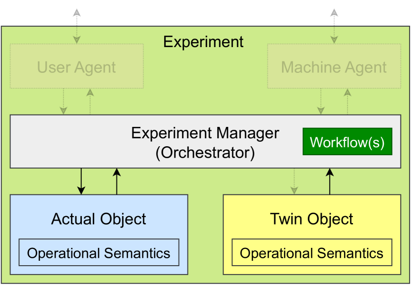
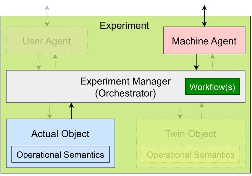
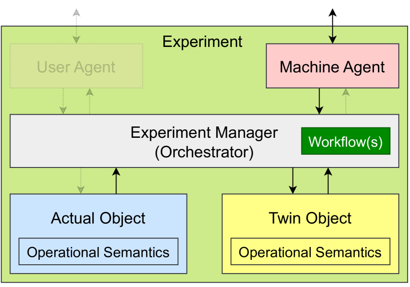
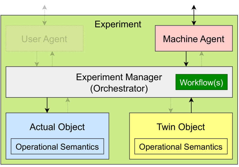
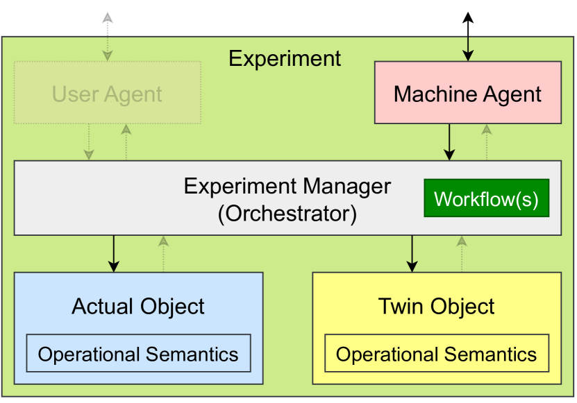
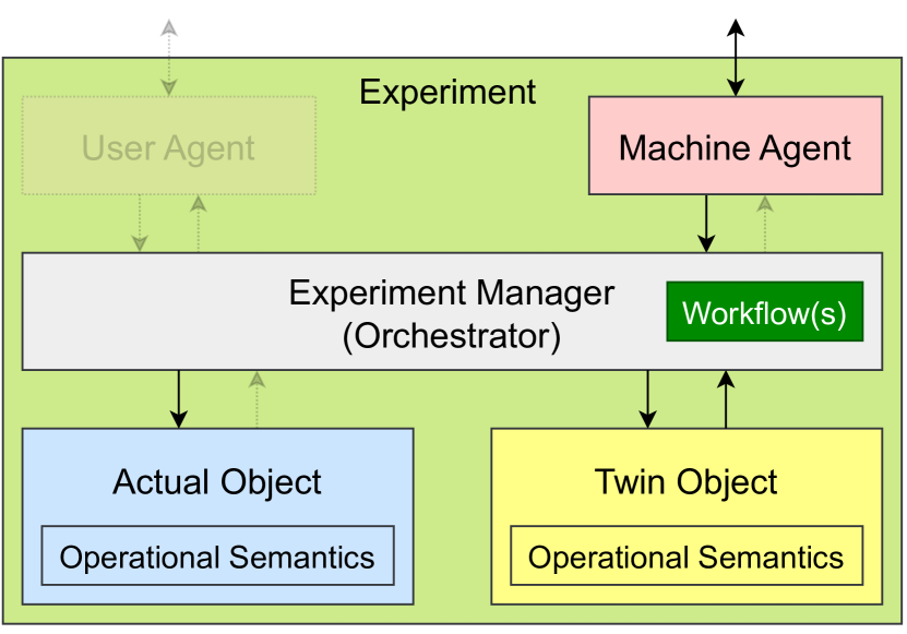
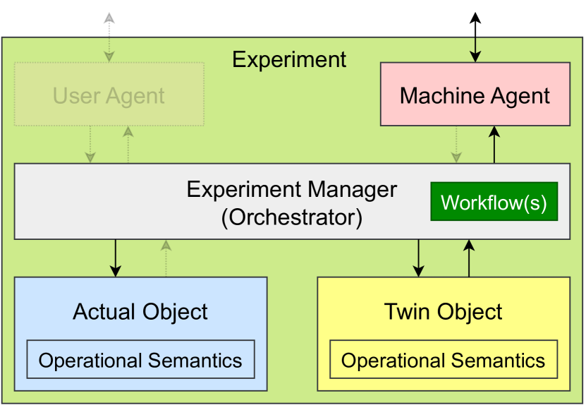
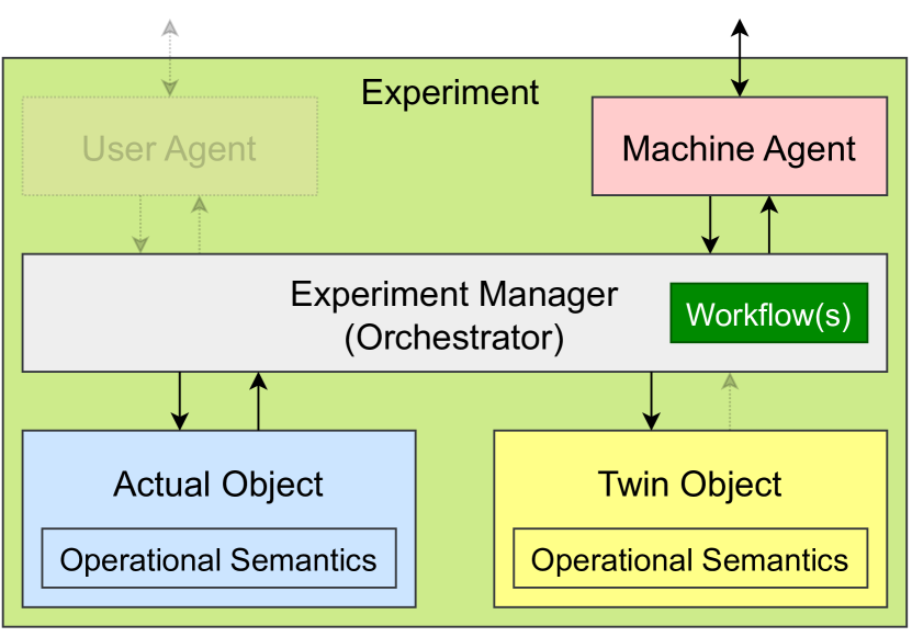
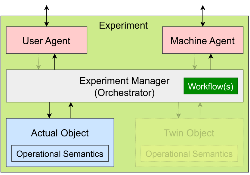
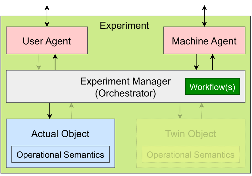
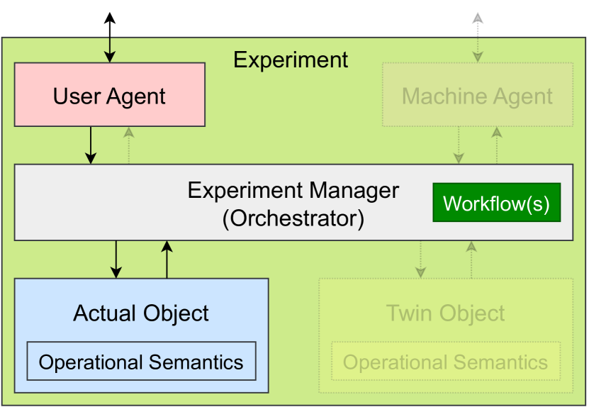
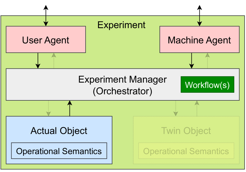
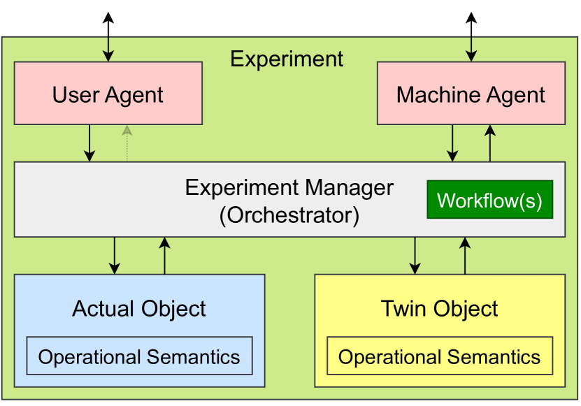
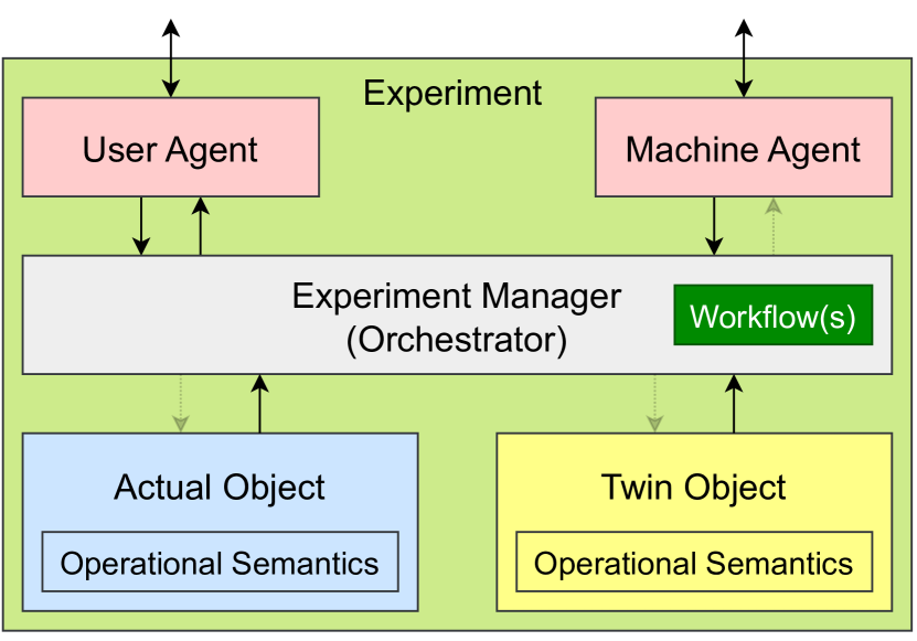
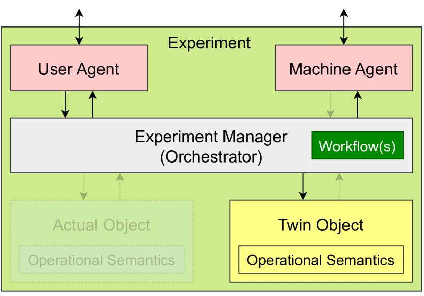
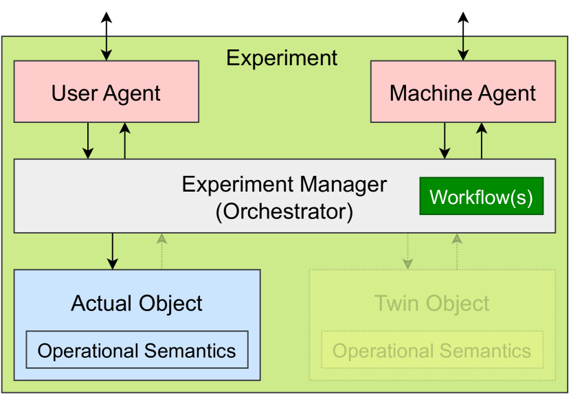
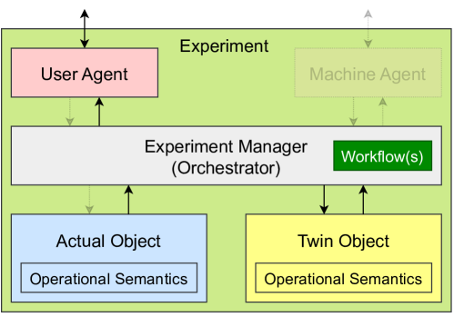
Figure 5 illustrates the basic architecture to which a multitude of existing twinning experiments conform. Notice that it is high-level and abstract, allowing users to decide on a high level which components to include in their system.
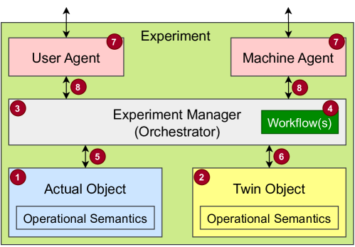
To further explain the figure, each component has been annotated with a number. The AO and TO are given a behaviour via its operational semantics. This can be a neural network, the execution of code, real-world behaviour, etc. It is important to denote that is an abstraction of a specific view of the actual world (and environment) in which the AO is active. is a so-called “Experiment Manger” (or “Orchestrator”) which contains a set of workflows that indicate how the experiment is to be executed. Because the experiment is created for a specific set of goals, this logic should also be contained in . For instance, if we only want to have a dashboard that visualizes the current state, the collection of this state is to be done by the Experiment Manager. If instead we want some anomaly detection, the Experiment Manager needs to compute some distance metric.
and indicate the communication between the Experiment Manager and the AO or TO, respectively. Note that the downwards communication may be interpreted in a really broad manner. It may consider the intructions that need to be sent to the objects, to launch or halt their individual executions. Alternatively, it may also send data to update the objects (for a DG, DS or DT). The upwards communication can be considered the set of data that the sensors in this AO have captured.
The Orchestrator can communicate with some User Agent or Machine Agent , which identifies an access point for a user or another system to obtain information about this experiment. This could be a dashboard, or an API. The communication between the Agents and the Orchestrator can be bidirectional when can also steer the twin, but it might likely be one-directional when discussing a DM or a DS.
The AO and the TO themselves (including their operational semantics) can be separated into more specific architectures, based on the desired goals w.r.t. their PoIs. This is illustrated in figure 6.
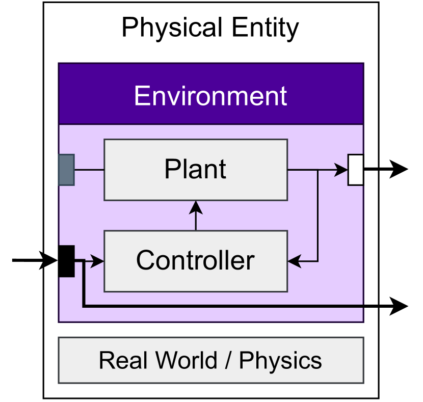
Commonly in a DT, the AO is a physical entity, which implies that it is a SuS that is active in the real, physical world. One possible architecture for such a real-world system, focusing on a plant-controller feedback loop is given in figure 6(a). This system is active in a (subset of) the real-world environment, which implies that this should also be incorporated in the entity. Additionally, there may be environmental influences we did not account for. For instance: a really sunny day might yield a sensor to produce invalid results. The operational semantics of this entity equates to its behaviour in the real-world (i.e., physics).
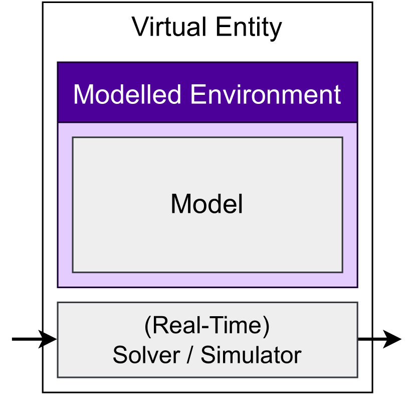
A DT has its TO in the virtual world, which is identified as a “virtual entity” in figure 6(b). Here, a model in some formalism is given operational semantics by executing a solver (or a simulator). This may potentially be a real-time simulator, or an as-fast-as-possible simulator, depending on the chosen goals.
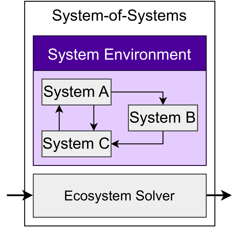
Figure 6(c) shows a system-of-systems setup. For instance, collaboration of multiple machines in a factory. If this is virtual, this will likely be solved using co-simulation. If it is in the real-world, its behaviour is the union of the sub-system behaviour, including the communications.
Hence, there is no requirement that the AO is a physical entity and the TO is a virtual entity. A plethora of other options exist (Paredis et al., 2024). It might as well be the case that the AO can itself be a virtual entity (Heithoff et al., 2023; Angjeliu et al., 2020), a biochemical entity (David et al., 2023; Howard et al., 2021; Tekinerdogan and Verdouw, 2020; Silber et al., 2023; Knibbe et al., 2022), a social entity (Graessler and Poehler, 2018; Traoré, 2023), an electromechanical entity (Barosan et al., 2020; Mandolla et al., 2019; Walravens et al., 2022), a solid entity (Dalibor et al., 2022), a system-of-systems (Biesinger et al., 2018), or a business process (Rambow-Hoeschele et al., 2018). Similarly, the TO also has the option to be a biochemical entity (Topuzoglu et al., 2019), a social entity, an electromechanical entity (Ferguson, 2020), or a solid entity (e.g., a sand table, or the Apollo training capsules).
For the AO, the incoming and outgoing arrows in figures 6(a), 6(b) and 6(c) relate to in figure 5. Similarly, for the TO, the incoming and outgoing arrows represent .
5.1. Common Architecture Variations
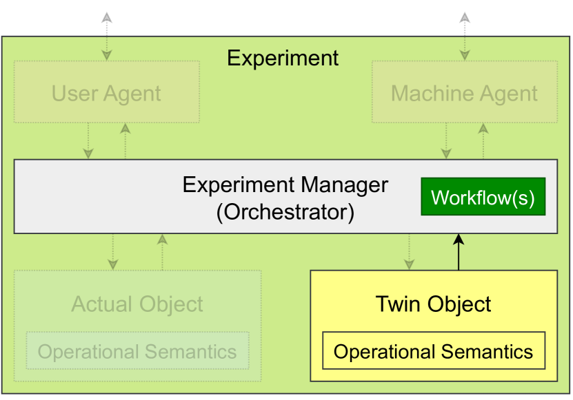
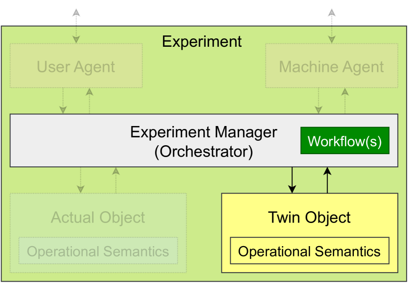
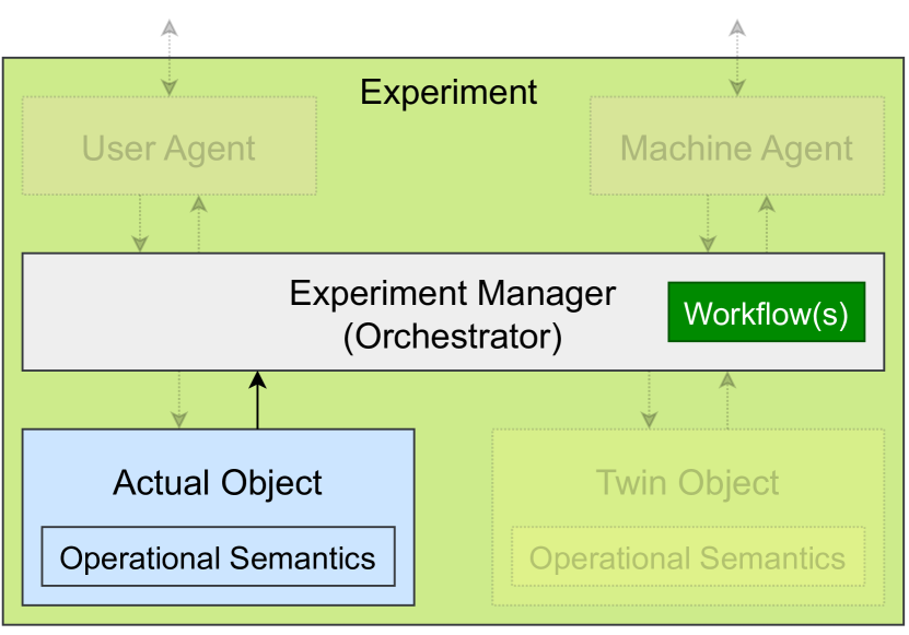
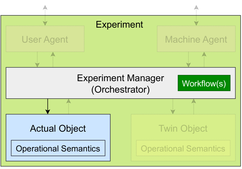
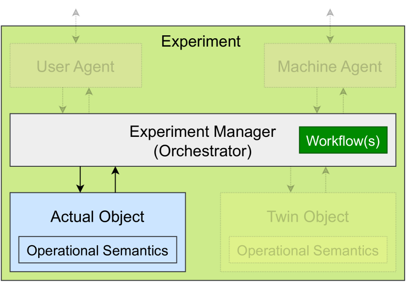
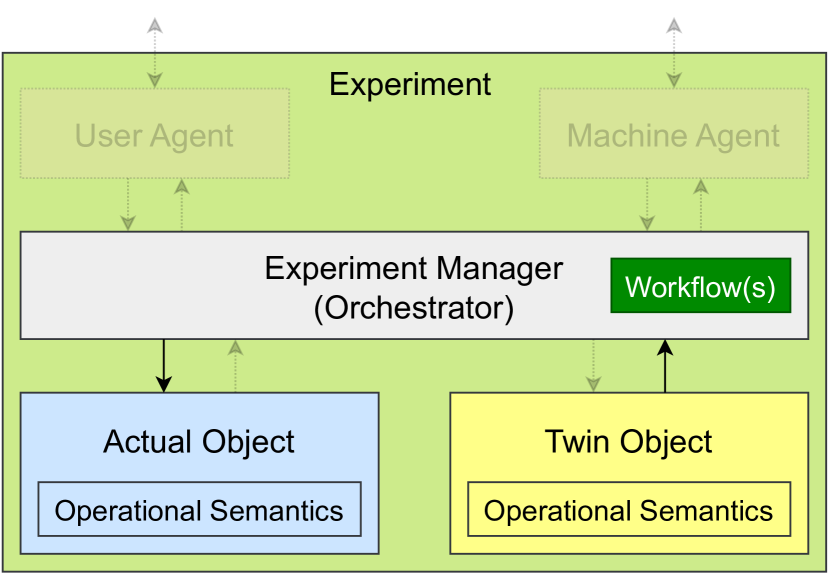
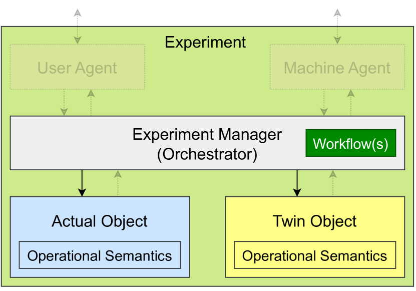
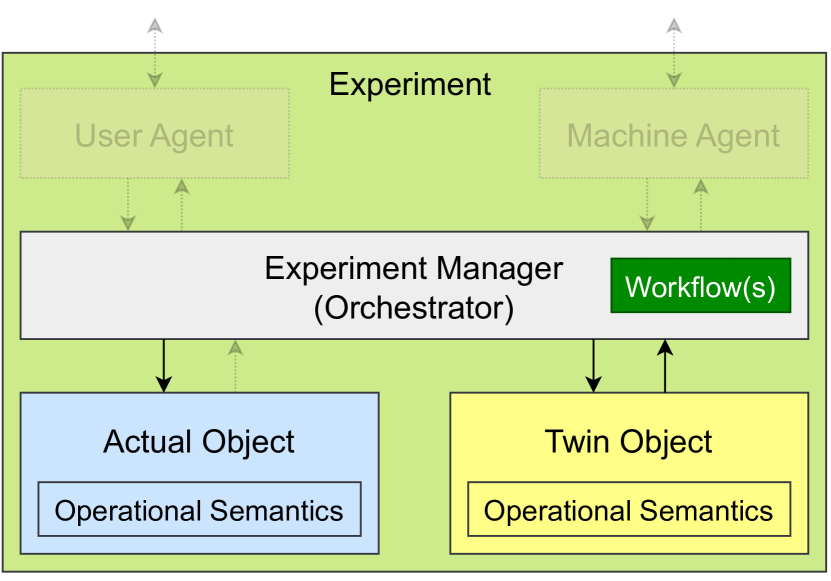
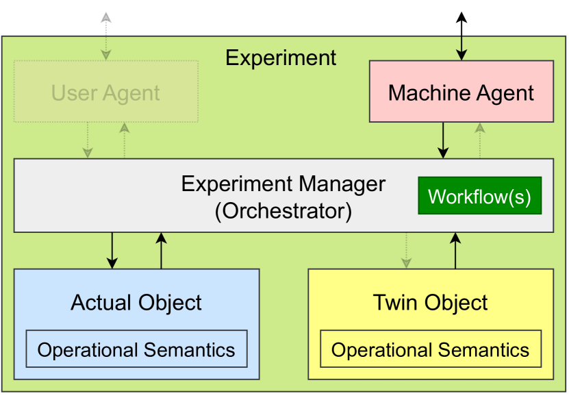
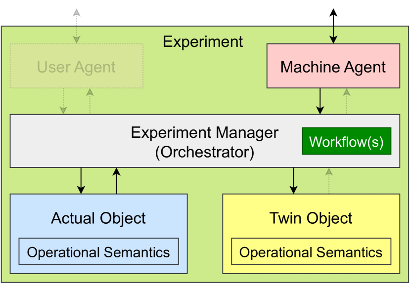
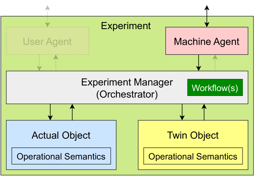
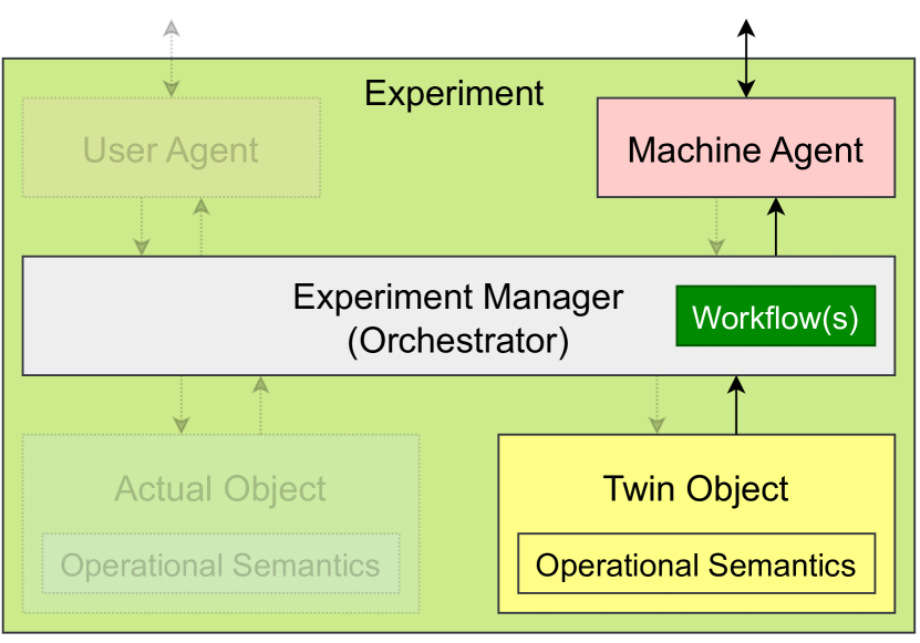
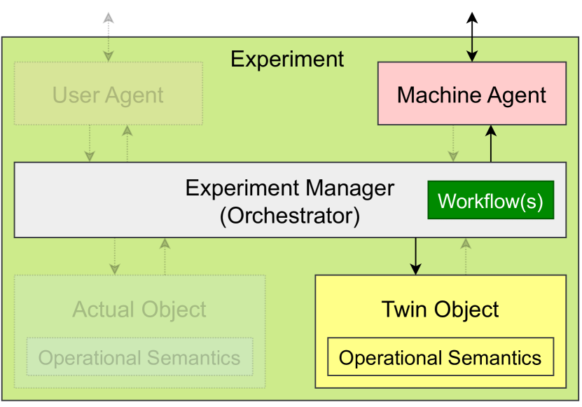
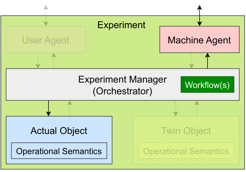
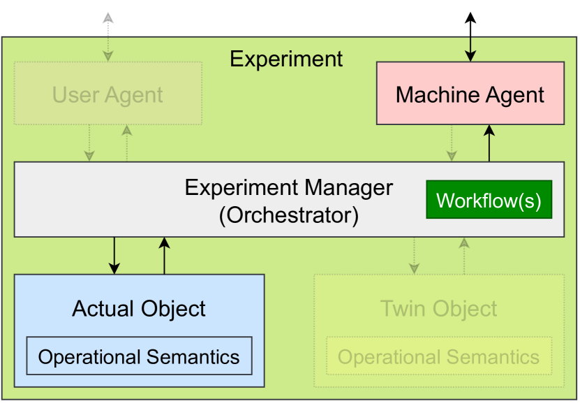
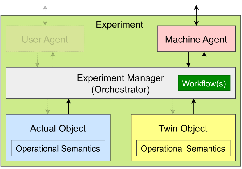
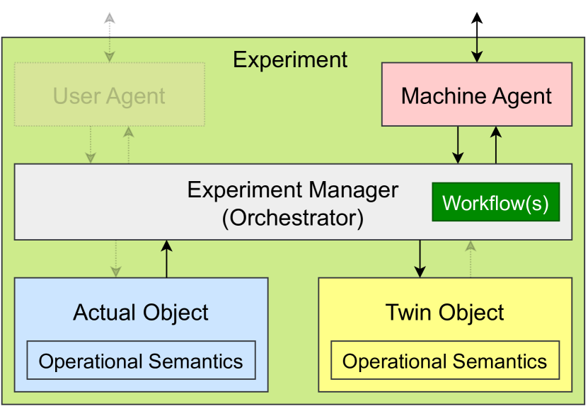
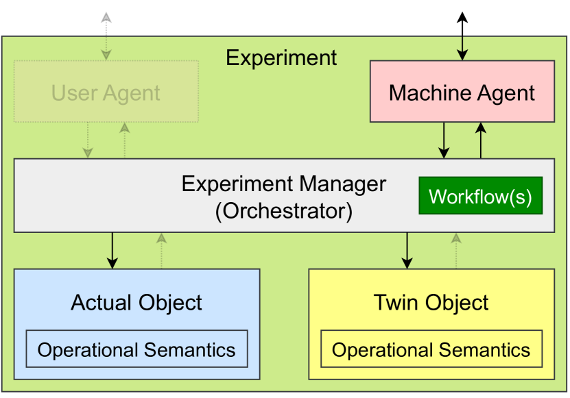
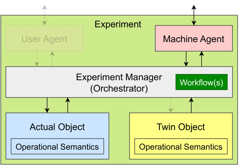
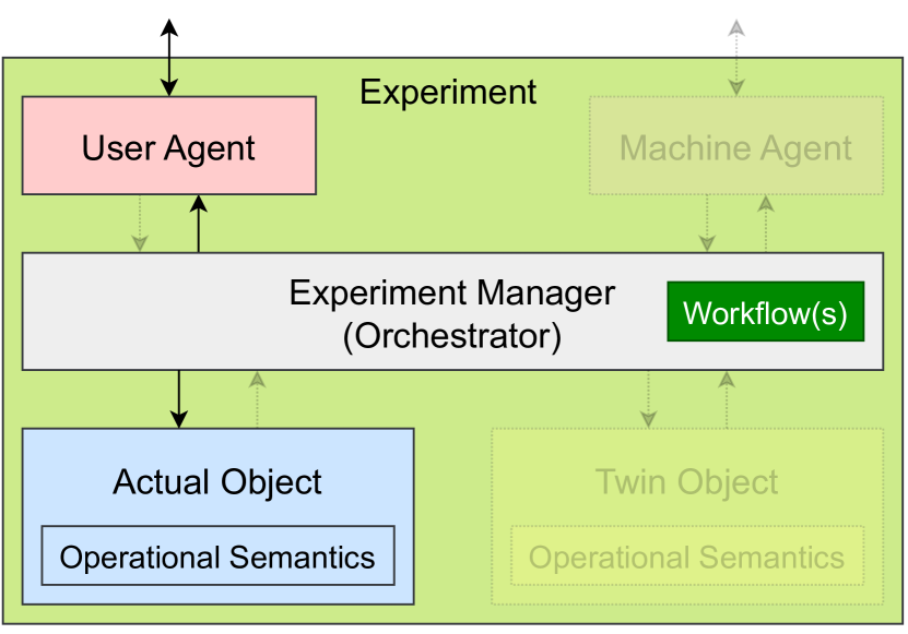
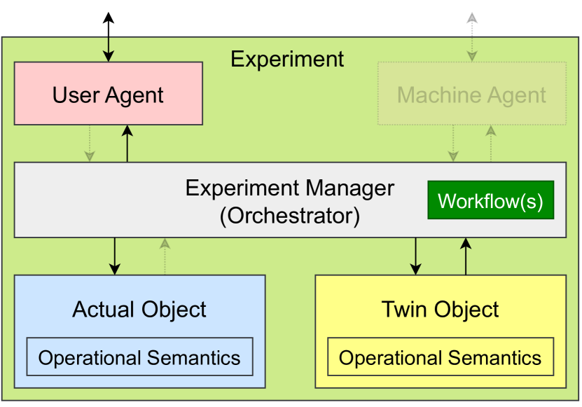
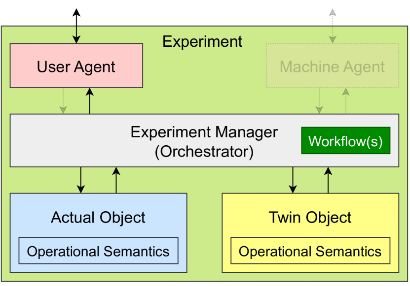
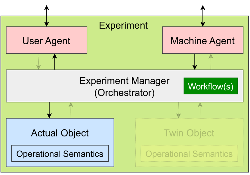
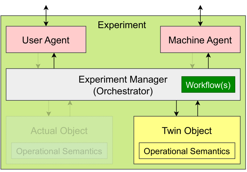
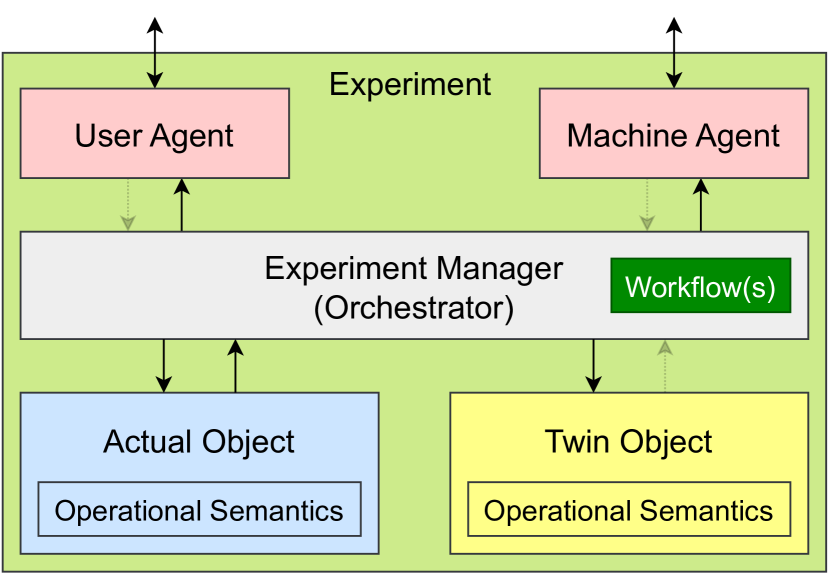
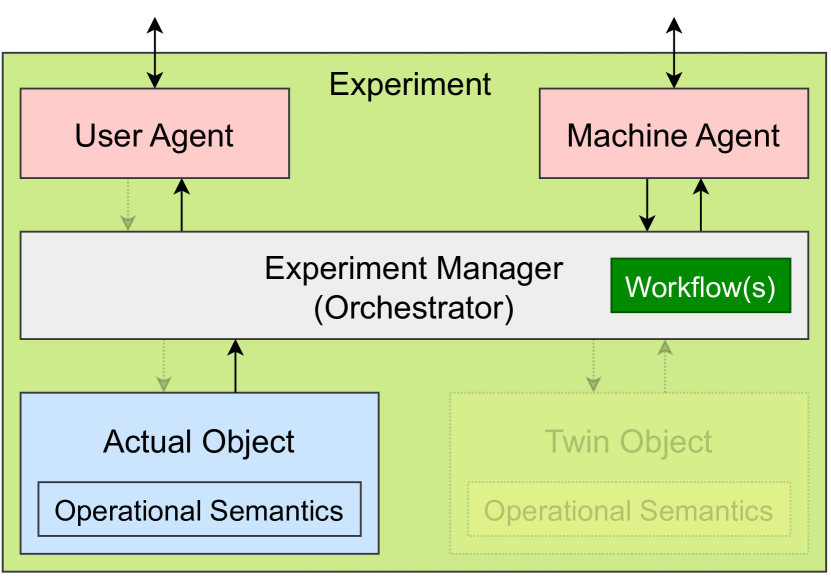
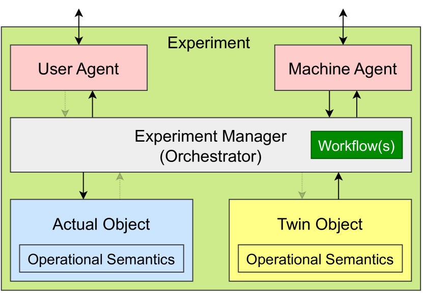
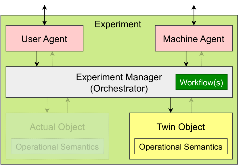
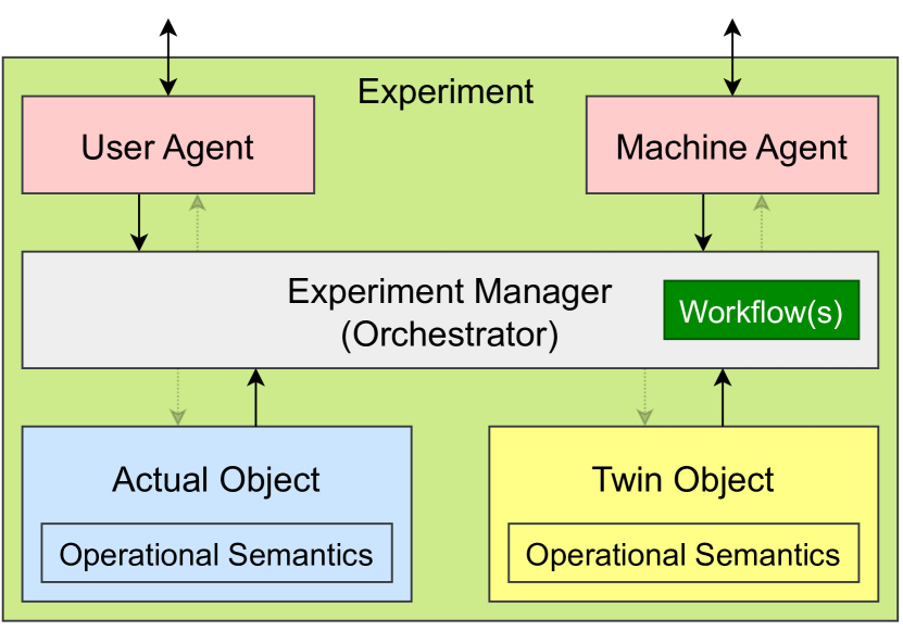
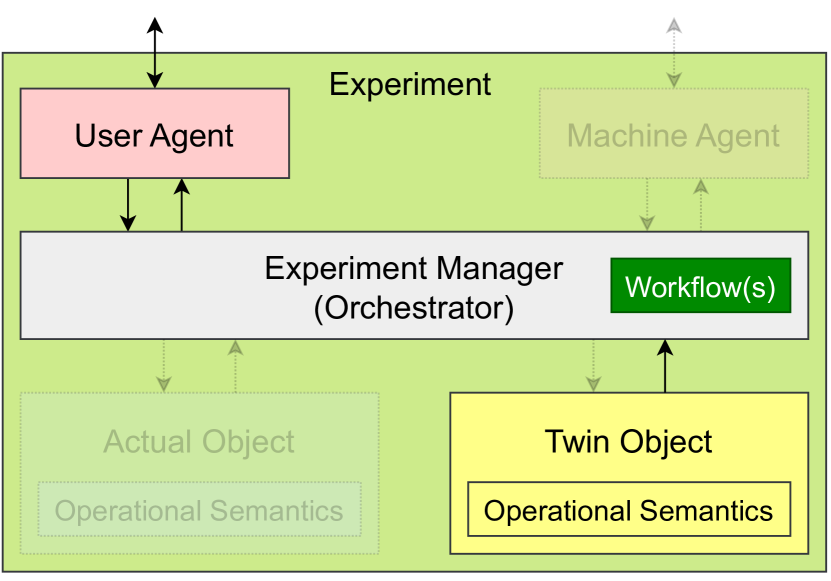
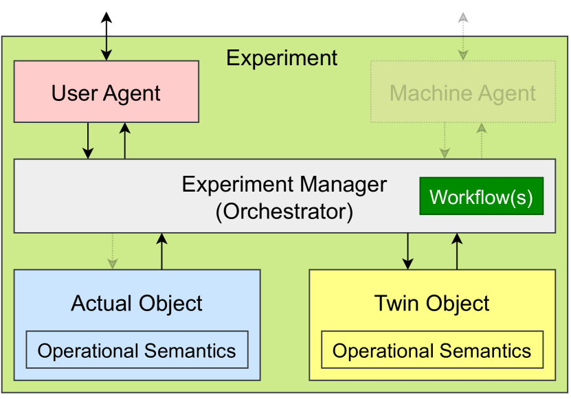
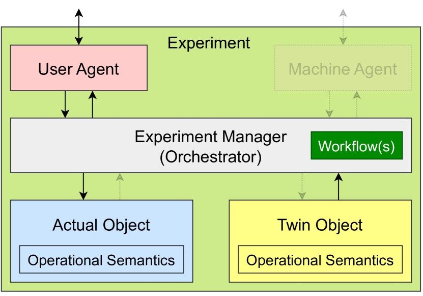
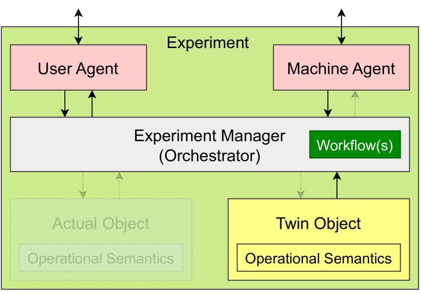
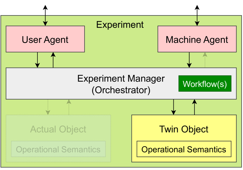
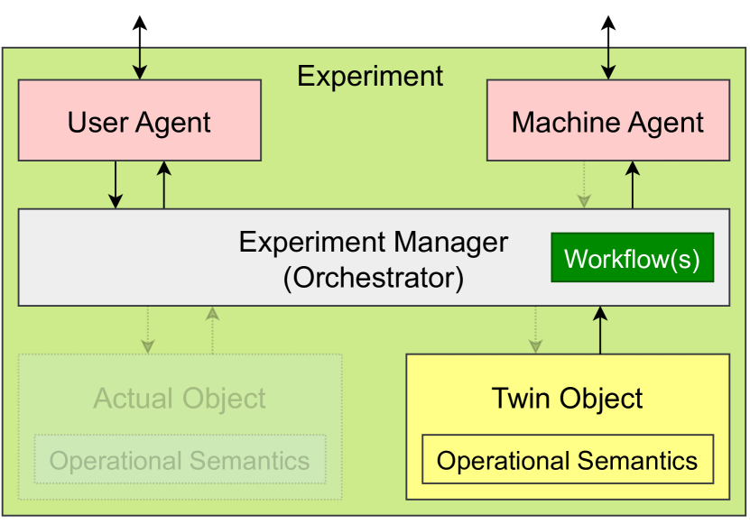
Appendix A shows all possible variations of the architecture shown in figure 5. Notice that at least an AO or a TO needs to be present and that all arrows need to be connected.
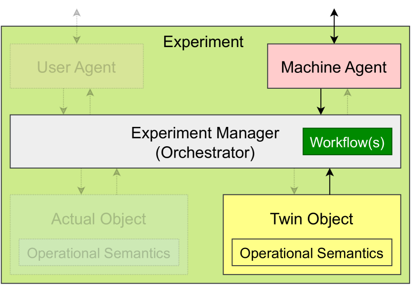
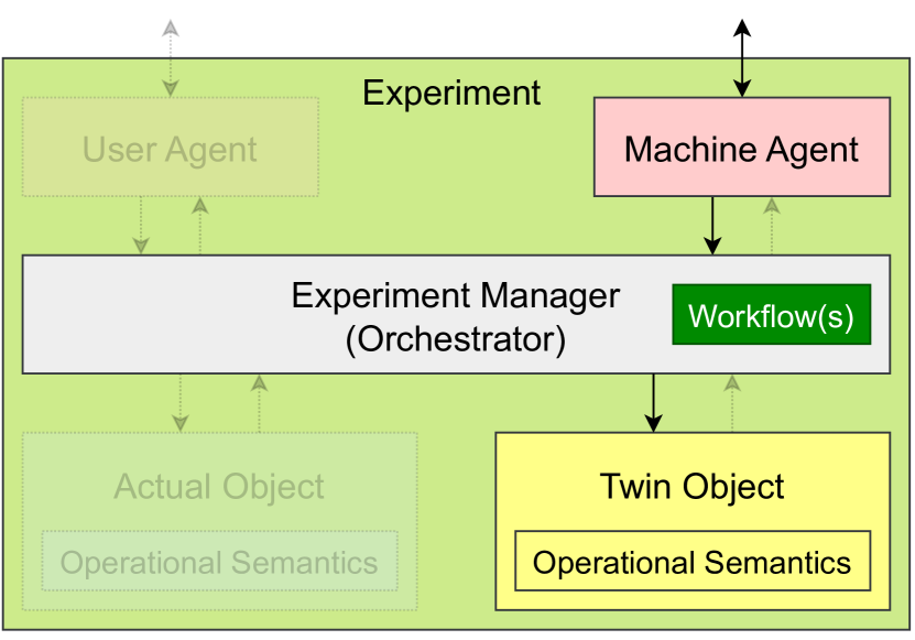
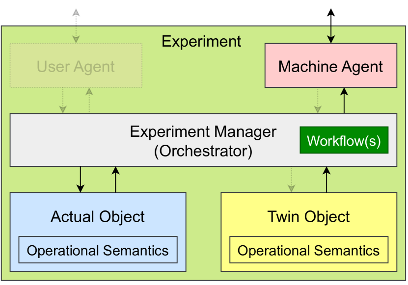
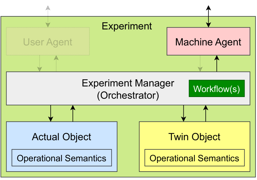
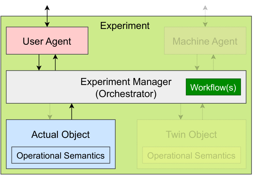
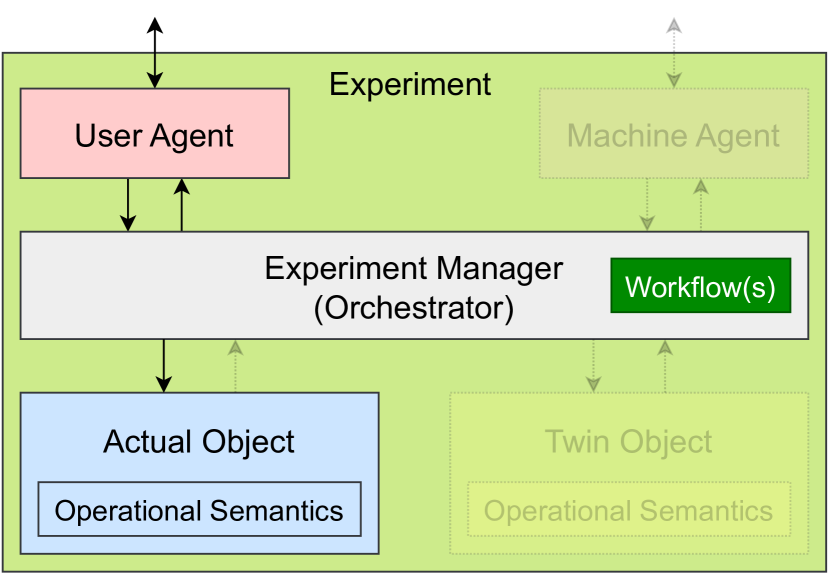
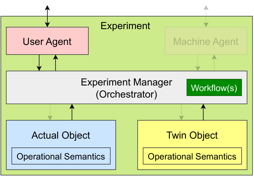
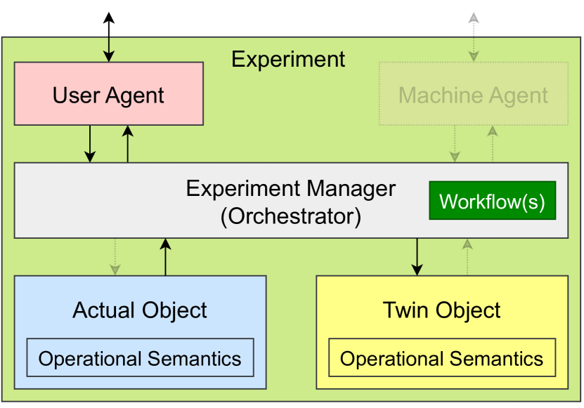
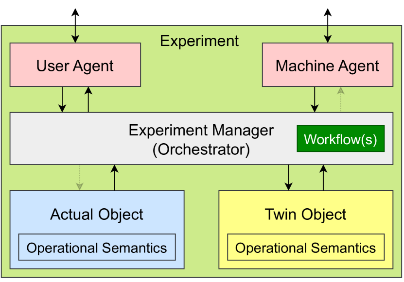
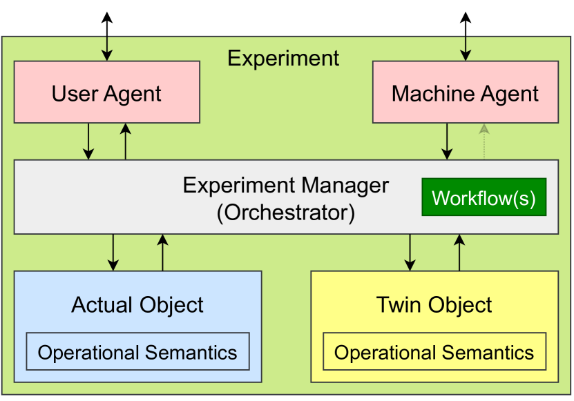
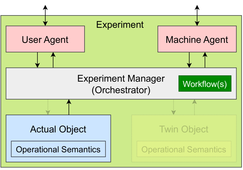
Commonly, a Machine Agent or a User Agent should be present. This only makes sense when the communication between the Machine/User Agent and the Orchestrator goes in the same direction as the communication between the Orchestrator and the AO and/or TO. For instance, figure 31 does not make sense, as the Machine Agent influences the Orchestrator, but the latter does not use this to update the TO. For the sake of readability, we will ignore the Machine Agent and User Agent in the further description (and thus only look at the first 15 variants).
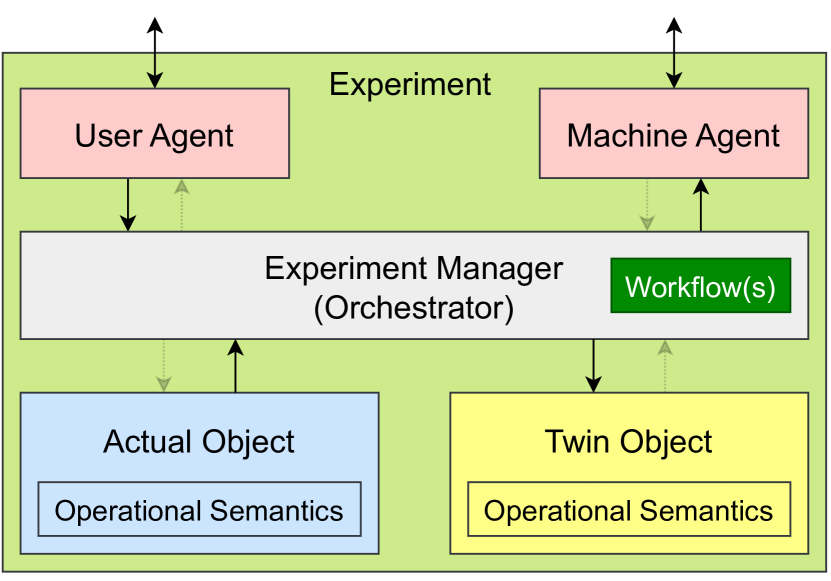
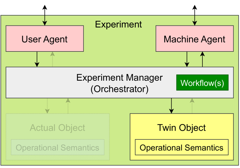
Figure 19, figure 19 and figure 19 show a simple simulation that can either be autonomous, instructed or both. Figure 19, figure 19 and figure 19 show the same for a running SuS.
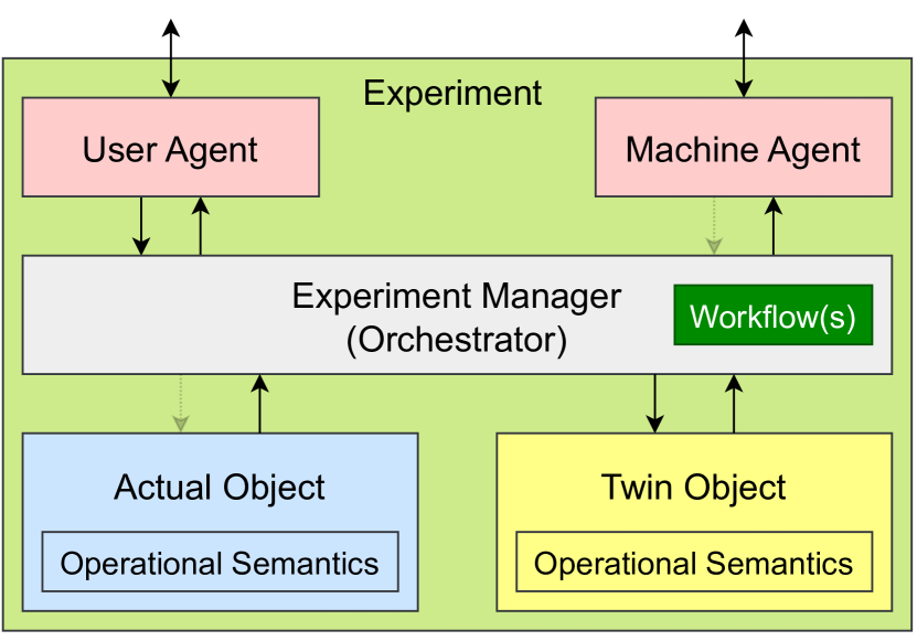
If we assume that all arrows represent data transfer (and not control information), we can identify an example of a Digital Model (as per (Kritzinger et al., 2018)) in figure 19. Figure 19 then shows a Digital Shadow and figure 31 is indicative of a Digital Generator (Tekinerdogan and Verdouw, 2020). Figure 31 is the minimal setup when we consider the Digital twin from (Kritzinger et al., 2018). Note that for the Digital Shadow, figure 19 makes more sense, given that the Orchestrator will also use information from the TO. The same can be said for the Digital Generator and figure 31.
5.2. Choices for Running Examples
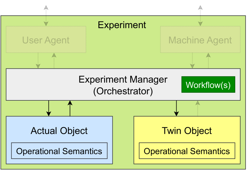
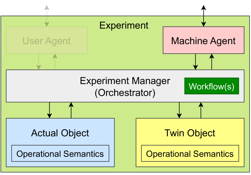
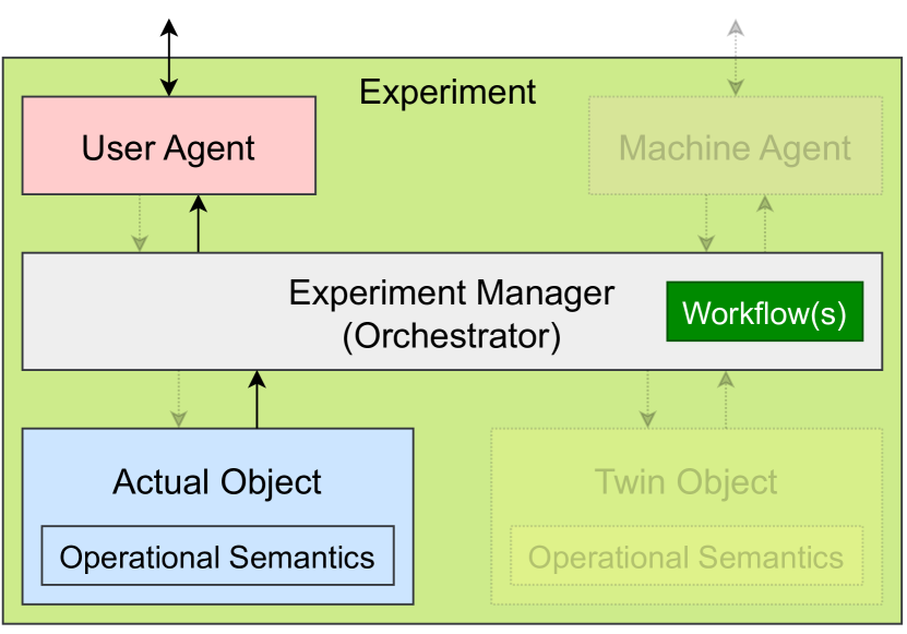
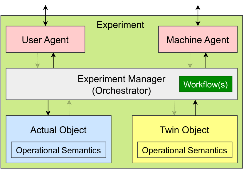
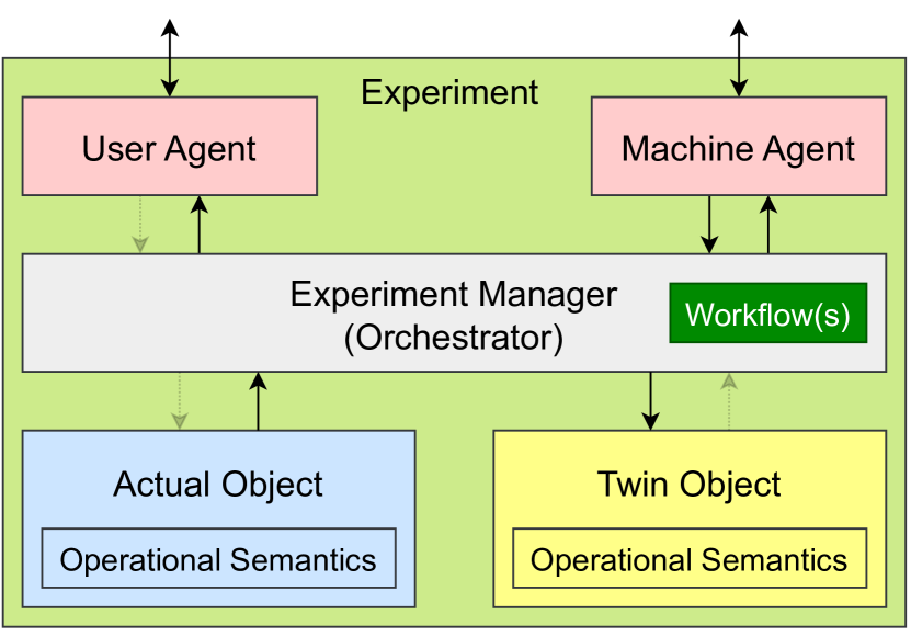
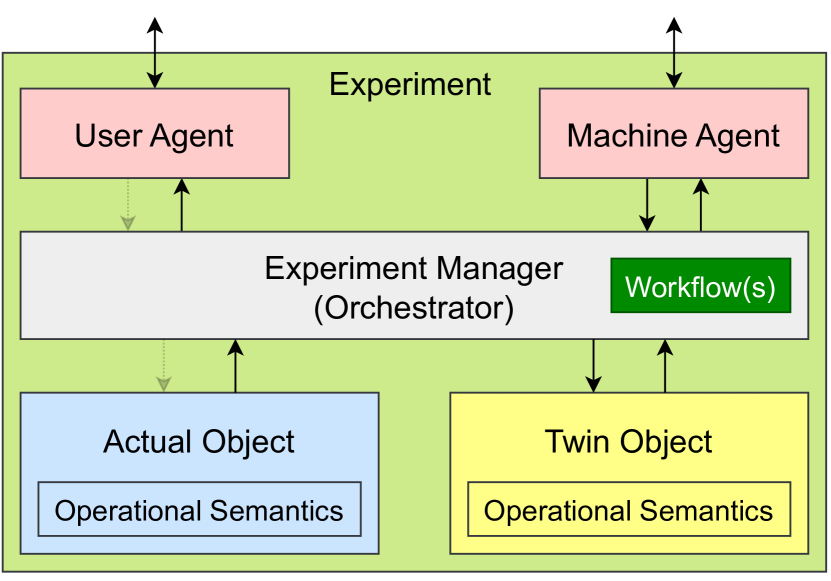
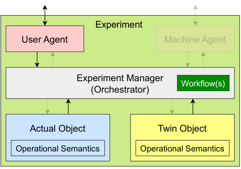
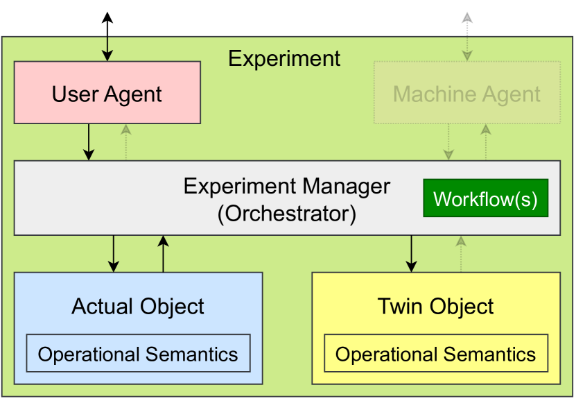
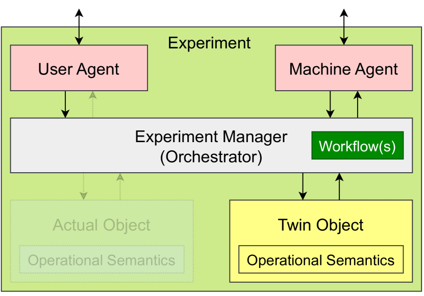
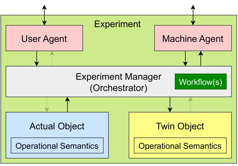
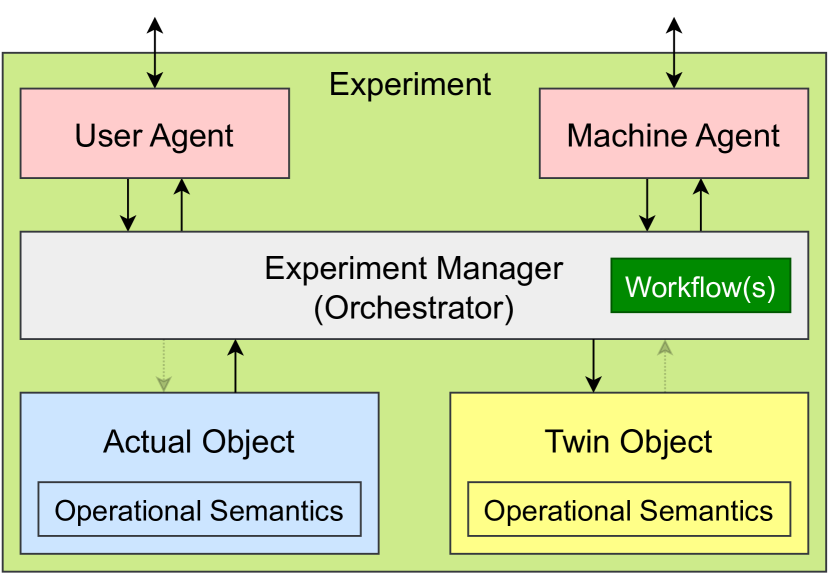
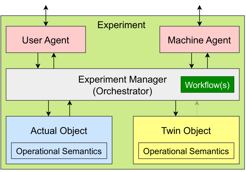
Based on the goal choices, made in table 1 and table 2, we can deduce that (for the use-cases), the architecture from figure 5 is to be altered to figure 7 and figure 8 (respectively).
The port example is a simple Digital Model, which implies data gathering from both the AO and the TO (via the Orchestrator). Additionally, the Orchestrator may also steer (i.e., setup, launch, progress, pause, halt, teardown,…) the TO. The real-time animation is made possible via the User Agent.

The port use-case is a very simple example, based on real-world information. For both the AO and the TO, figure 6(b) will be used.
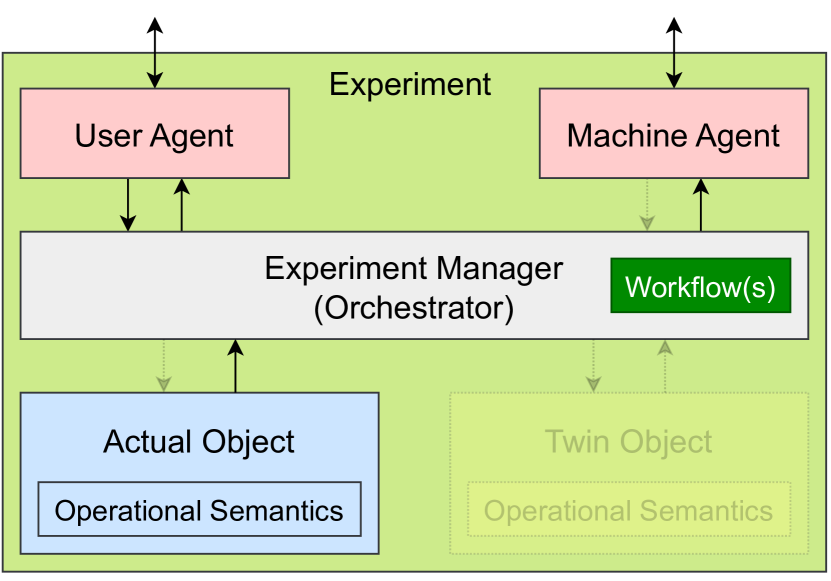
The yacht example is a Digital Shadow, which implies that besides data gathering, there is also data transfer between the AO and the TO. Whereas the AO will exist in the physical space, it is a simplification of reality, resulting in figure 6(b) for both the AO and the TO. Inside the model, however, a plant-controller loop is constructed, to mimic the behaviour shown in figure 6(a).
Within the COOCK project, PoAB provided access to data from their APICS system, yielding a data lake with information for all activities of tugboats in 2022. This data contains a real-world execution trace and can hence be used as AO (i.e., a representation of reality) if desired.
6. Deployment
In order to deploy the ship experiment, we will use the architecture from figure 7 as a basis to know which components to construct. Yet, there are still some technological decisions to be made. Besides the selection of the modelling languages, tools, simulators, formalisms and exact implementation of the models, we still need to decide the Operating System (OS) on which we will deploy the components and the exact communication protocols.
Common OS choices are Windows, Apple, or Linux, but all their versions and flavours can also be considered. This choice is less important when tools are platform-independent, but this is definitely not always the case. Specific devices might have a very small OS with limited memory, disabling the possibility of memory-intensive computations (such as most geometric mathematics) that might be required to accomplish a specific goal. When the AO and/or TO is not in the virtual space, we need to consider the real-world location where it is situated. A twin that focuses on the very specific light intensity of a sensor might be massively influenced by the amount of sunshine during the experiment.
For communication protocols, common standards for twinning are DDS (https://www.rti.com/products/dds-standard), MQTT (https://mqtt.org/) and OPC-UA (https://opcfoundation.org/about/opc-technologies/opc-ua/). When components are present on the same device, maybe the communication might happen via shared memory. Alternatively, classic distributed computing protocols (like client-server and Peer to Peer (P2P)) might also be an option, likely implemented over HTTP, TCP/IP or UDP. When working with robots, the industrial standard is ROS (https://www.ros.org/), which is a DDS-based technology. In the real world it is possible to use indicator lights, displays, Morse code, flag semaphores, speech,…in order to convey information. Each of these technologies has its own advantages and downsides, making selecting “the right one” for your goal(s) an important question.
6.1. Choices for Running Examples
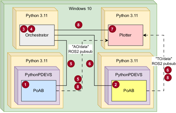
For the port, we decided on using DEVS to model the PoAB system, such that we can implement it in PythonPDEVS (Van Tendeloo and Vangheluwe, 2015), which allows real-time execution of the simulation. A mapping tool called geoplotlib is used to do the visualization of the port. All communication happens via ROS2 (galactic geochelone). A deployment diagram is shown in figure 9, following the same numbering annotations as figure 5.
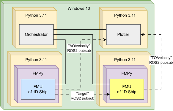
The yacht example uses ODEs that can be modelled using Modelica. We will use this to model both the AO and the TO, following a standard plant-controller pattern. Next, these models are converted to FMUs, which can easily be co-simulated. A user-agent written in Python can visualize certain system states via the FMU interface. As a communication protocol, we will use ROS2 (galactic geochelone) for all communications. A deployment diagram is shown in figure 10.
7. Conclusions and Future Work
Nowadays, industry is heavily focused on Industry 4.0 and DTs. This twinning paradigm can be applied in any domain to answer specific research questions. Hence, a vast product family of twinning experiments appears. This paper highlights three high-level phases on which variability may appear: Problem Space Goal Construction, Designing Architectures and Deployment.
We can construct a large feature tree based on existing sets of goals (Dalibor et al., 2022; Paredis et al., 2024). Based on these choices, a lot of implementation details are already made explicit.
A lot of conceptual architectures already exist. Some focus on the connectivity (Kritzinger et al., 2018), others emphasise on the system flow (Eramo et al., 2021), whereas others mainly focus on the internal components of the TO itself (Bolender et al., 2021). This paper focuses on the variability that exists between the most common architectural descriptions. Next, this architecture is deployed as a running system, making even more choices on the used formalisms and technologies.
The use-case described in this paper entails a simplistic “toy” scenario. In the future, more complicated (and real-world) use-cases may be used to show and verify the validity of the provided architecture. Furthermore, we can take a look at the architecture within the context of twinning ecosystems. Finally, we are planning on showing the equivalence between the architecture and the previously mentioned conceptual architectures that also have appeared in literature.
Acknowledgements.
We would like to thank the Port of Antwerp-Bruges for their explanations of the internal workings of the nautical chain.References
- (1)
- Angjeliu et al. (2020) Grigor Angjeliu, Dario Coronelli, and Giuliana Cardani. 2020. Development of the simulation model for Digital Twin applications in historical masonry buildings: The integration between numerical and experimental reality. Computers & Structures 238 (2020), 106282. https://doi.org/10.1016/j.compstruc.2020.106282
- Barosan et al. (2020) Ion Barosan, Arash Arjmandi Basmenj, Sudhanshu GR Chouhan, and David Manrique. 2020. Development of a Virtual Simulation Environment and a Digital Twin of an Autonomous Driving Truck for a Distribution Center. In European Conference on Software Architecture. Springer, 542–557.
- Biesinger et al. (2018) Florian Biesinger, Davis Meike, Benedikt Kraß, and Michael Weyrich. 2018. A Case Study for a Digital Twin of Body-in-White Production Systems General Concept for Automated Updating of Planning Projects in the Digital Factory. In 2018 IEEE 23rd International Conference on Emerging Technologies and Factory Automation (ETFA) (Torino, Italy). IEEE Press, 19–26. https://doi.org/10.1109/ETFA.2018.8502467
- Bolender et al. (2021) Tim Bolender, Gereon Bürvenich, Manuela Dalibor, Bernhard Rumpe, and Andreas Wortmann. 2021. Self-adaptive manufacturing with digital twins. In 2021 International Symposium on Software Engineering for Adaptive and Self-Managing Systems (SEAMS). IEEE, 156–166.
- Boss et al. (2020) B Boss, S Malakuti, SW Lin, T Usländer, E Clauer, M Hoffmeister, and L Stojanovic. 2020. Digital twin and asset administration shell concepts and application in the industrial internet and industrie 4.0. Industrial Internet Consortium: Boston, MA, USA (2020).
- Dalibor et al. (2022) Manuela Dalibor, Nico Jansen, Bernhard Rumpe, David Schmalzing, Louis Wachtmeister, Manuel Wimmer, and Andreas Wortmann. 2022. A Cross-Domain Systematic Mapping Study on Software Engineering for Digital Twins. Journal of Systems and Software 193 (2022), 111361. https://doi.org/10.1016/j.jss.2022.111361
- David et al. (2023) Istvan David, Pascal Archambault, Quentin Wolak, Cong Vinh Vu, Timothé Lalonde, Kashif Riaz, Eugene Syriani, and Houari Sahraoui. 2023. Digital Twins for Cyber-Biophysical Systems: Challenges and Lessons Learned. In ACM/IEEE 26th International Conference on Model-Driven Engineering Languages and Systems (MODELS). IEEE.
- Eramo et al. (2021) Romina Eramo, Francis Bordeleau, Benoit Combemale, Mark van Den Brand, Manuel Wimmer, and Andreas Wortmann. 2021. Conceptualizing digital twins. IEEE Software (2021).
- Ferguson (2020) Stephen Ferguson. 2020. Apollo 13: The First Digital Twin. https://blogs.sw.siemens.com/simcenter/apollo-13-the-first-digital-twin/ Accessed: February 7th 2024.
- Graessler and Poehler (2018) Iris Graessler and Alexander Poehler. 2018. Intelligent control of an assembly station by integration of a digital twin for employees into the decentralized control system. Procedia Manufacturing 24 (2018), 185–189. https://doi.org/10.1016/j.promfg.2018.06.041 4th International Conference on System-Integrated Intelligence: Intelligent, Flexible and Connected Systems in Products and Production.
- Grieves and Vickers (2017) Michael Grieves and John Vickers. 2017. Digital twin: Mitigating unpredictable, undesirable emergent behavior in complex systems. In Transdisciplinary perspectives on complex systems. Springer, 85–113.
- Heithoff et al. (2023) Malte Heithoff, Alexander Hellwig, Judith Michael, and Bernhard Rumpe. 2023. Digital Twins for Sustainable Software Systems. In Int. Workshop on Green and Sustainable Software (GREENS 2023). IEEE.
- Howard et al. (2021) Daniel Anthony Howard, Zheng Ma, Christian Veje, Anders Clausen, Jesper Mazanti Aaslyng, and Bo Nørregaard Jørgensen. 2021. Greenhouse industry 4.0–digital twin technology for commercial greenhouses. Energy Informatics 4, 2 (2021), 1–13.
- Jones et al. (2020) David Jones, Chris Snider, Aydin Nassehi, Jason Yon, and Ben Hicks. 2020. Characterising the Digital Twin: A systematic literature review. CIRP Journal of Manufacturing Science and Technology 29 (2020), 36–52. https://doi.org/10.1016/j.cirpj.2020.02.002
- Kang et al. (1990) Kyo C. Kang, Sholom G. Cohen, James A. Hess, William E. Novak, and A. Spencer Peterson. 1990. Feature-oriented domain analysis (FODA) feasibility study. Technical Report. Carnegie Mellon University.
- Knibbe et al. (2022) Willem Jan Knibbe, Lydia Afman, Sjoerd Boersma, Marc-Jeroen Bogaardt, Jochem Evers, Frits van Evert, Jene van der Heide, Idse Hoving, Simon van Mourik, Dick de Ridder, and Allard de Wit. 2022. Digital twins in the green life sciences. NJAS: Impact in Agricultural and Life Sciences 94, 1 (2022), 249–279. https://doi.org/10.1080/27685241.2022.2150571 arXiv:https://doi.org/10.1080/27685241.2022.2150571
- Kritzinger et al. (2018) Werner Kritzinger, Matthias Karner, Georg Traar, Jan Henjes, and Wilfried Sihn. 2018. Digital Twin in Manufacturing: A Categorical Literature Review and Classification. IFAC-PapersOnLine 51, 11 (2018), 1016–1022.
- Mandolla et al. (2019) Claudio Mandolla, Antonio Messeni Petruzzelli, Gianluca Percoco, and Andrea Urbinati. 2019. Building a digital twin for additive manufacturing through the exploitation of blockchain: A case analysis of the aircraft industry. Computers in Industry 109 (2019), 134–152.
- Paredis et al. (2021) Randy Paredis, Cláudio Gomes, and Hans Vangheluwe. 2021. Towards a Family of Digital Model / Shadow / Twin Workflows and Architectures. In Proceedings of the 2nd International Conference on Innovative Intelligent Industrial Production and Logistics (IN4PL 2021). SCITEPRESS – Science and Technology Publications, Lda., 174–182.
- Paredis and Vangheluwe (2022) Randy Paredis and Hans Vangheluwe. 2022. Towards a Digital Z Framework Based on a Family of Architectures and a Virtual Knowledge Graph. In Proceedings of the 25th International Conference on Model Driven Engineering Languages and Systems (MODELS).
- Paredis et al. (2024) Randy Paredis, Hans Vangheluwe, and Pamela Adelino Ramos Albertins. 2024. COOCK project Smart Port 2025 D3.1: ”To Twin Or Not To Twin”. Technical Report. University of Antwerp. arXiv:2401.12747 [eess.SY]
- Qamar and Paredis (2012) Ahsan Qamar and Christiaan Paredis. 2012. Dependency Modeling And Model Management In Mechatronic Design, In Proceedings of the ASME Design Engineering Technical Conference. Proceedings of the ASME Design Engineering Technical Conference 2. https://doi.org/10.1115/DETC2012-70272
- Rambow-Hoeschele et al. (2018) Kira Rambow-Hoeschele, Anna Nagl, David K. Harrison, Bruce M. Wood, Karlheinz Bozem, Kevin Braun, and Peter Hoch. 2018. Creation of a Digital Business Model Builder. 2018 IEEE International Conference on Engineering, Technology and Innovation (ICE/ITMC) (2018), 1–7. https://api.semanticscholar.org/CorpusID:52018061
- Silber et al. (2023) Klara Silber, Peter Sagmeister, Christine Schiller, Jason D Williams, Christopher A Hone, and C Oliver Kappe. 2023. Accelerating reaction modeling using dynamic flow experiments, part 2: development of a digital twin. Reaction Chemistry & Engineering 8, 11 (2023), 2849–2855.
- Tao and Zhang (2017) Fei Tao and Meng Zhang. 2017. Digital twin shop-floor: a new shop-floor paradigm towards smart manufacturing. Ieee Access 5 (2017), 20418–20427.
- Tekinerdogan and Verdouw (2020) Bedir Tekinerdogan and Cor Verdouw. 2020. Systems architecture design pattern catalog for developing digital twins. Sensors 20, 18 (2020), 5103.
- Topuzoglu et al. (2019) Tayfun Topuzoglu, Gülden Köktürk, Didem Akyol Altun, Aylin Sendemir, Ozge Andic Cakır, Ayca Tokuc, and Feyzal Avci Ozkaban. 2019. Finding the Shortest Paths in Izmir Map by Using Slime Molds Images. In 2019 International Conference on Control, Artificial Intelligence, Robotics & Optimization (ICCAIRO). IEEE, 202–206.
- Traoré (2023) Mamadou Kaba Traoré. 2023. High-Level Architecture for Interoperable Digital Twins. Preprints (October 2023). https://doi.org/10.20944/preprints202310.0659.v1
- Van Den Brand et al. (2021) Mark Van Den Brand, Loek Cleophas, Raghavendran Gunasekaran, Boudewijn Haverkort, David A Manrique Negrin, and Hossain Muhammad Muctadir. 2021. Models Meet Data: Challenges to Create Virtual Entities for Digital Twins. In 2021 ACM/IEEE International Conference on Model Driven Engineering Languages and Systems Companion (MODELS-C). IEEE, 225–228.
- Van der Valk et al. (2020) Hendrik Van der Valk, Hendrik Haße, Frederik Möller, Michael Arbter, Jan-Luca Henning, and Boris Otto. 2020. A Taxonomy of Digital Twins. In AMCIS.
- Van Tendeloo and Vangheluwe (2015) Yentl Van Tendeloo and Hans Vangheluwe. 2015. PythonPDEVS: a Distributed Parallel DEVS simulator. In Proceedings of the 2015 Spring Simulation Multiconference (12-15 April 2015). Alexandria, VA, USA, 844–851.
- Walravens et al. (2022) Gijs Walravens, Hossain Muhammad Muctadir, and Loek Cleophas. 2022. Virtual Soccer Champions: A Case Study on Artifact Reuse in Soccer Robot Digital Twin Construction. In Proceedings of the 25th International Conference on Model Driven Engineering Languages and Systems: Companion Proceedings (Montreal, Quebec, Canada) (MODELS ’22). ACM, 463–467. https://doi.org/10.1145/3550356.3561586
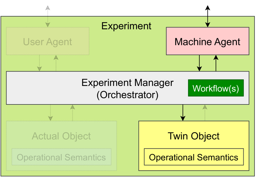
Appendix A Architectural Variability
List of all architectural variations for the given image. Removed components are faded out.