Well-Balanced Hydrodynamics for the Piecewise Parabolic Method with Characteristic Tracing

Michael Zingale Department of Physics and Astronomy, Stony Brook University, Stony Brook, NY 11794-3800, USA Michael Zingale michael.zingale@stonybrook.edu
Abstract

Well-balanced reconstruction techniques have been developed for stellar hydrodynamics to address the challenges of maintaining hydrostatic equilibrium during evolution. I show how to adapt a simple well-balanced method to the piecewise parabolic method for hydrodynamics. A python implementation of the method is provided.

hydrodynamics—methods: numerical
software: matplotlib (Hunter, 2007), numpy (van der Walt et al., 2011)

1 Introduction

The piecewise parabolic method (PPM) (Colella & Woodward, 1984) is widely used in astrophysical hydrodynamic simulation codes due to its low numerical viscosity. PPM reconstructs data on a grid as parabolas and integrates under them to accumulate the information that can make it to an interface over a timestep—this procedure is called characteristic tracing. This is then used to compute the fluxes through the zones and update the state in time. An alternative to characteristic tracing is a method-of-lines discretization, where the parabolic reconstruction is only used to find the value on the interface, and the time integration is treated as a system of ordinary differential equations.

A common problem with stellar hydrodynamics is maintaining hydrostatic equilibrium (HSE)—this requires the exact cancellation of the pressure gradient and the gravitational source, otherwise an acceleration will be generated. Well-balanced methods take the hydrostatic profile into account when doing the reconstruction. Recent techniques (Käppeli & Mishra, 2016; Käppeli, 2022) have shown how to achieve HSE to machine precision, but these focus piecewise linear reconstruction and method-of-lines integration. Here I demonstrate how to apply the same ideas to the original characteristic tracing formulation of PPM.

2 Well-Balanced PPM

PPM reconstruction works with the primitive variable formulation of the Euler equations:

$${\bf q}_{t}+{\bf A}({\bf q}){\bf q}_{x}+{\bf H}$$ (1)

where ${\bf q}=(\rho,u,p)^{\intercal}$ (density, velocity, and pressure), ${\bf H}=(0,g,0)^{\intercal}$ is the gravitational source term, ${\bf A}$ is

$${\bf A}=\left(\begin{array}[]{ccc}u&\rho&0\\ 0&u&1/\rho\\ 0&\Gamma_{1}p&u\end{array}\right)$$ (2)

and $\Gamma_{1}$ is the adiabatic index. The goal is to predict the values of ${\bf q}$ on each side of each interface separating the zones and then compute the flux through the zones by solving a Riemann problem. This interface state prediction, described in Colella & Woodward (1984), proceeds as:

  1. 1.

    Use a conservative cubic interpolant to find the interface values ${\bf q}$. I’ll write this as ${\bf q}_{i+1/2}=f({\bf q}_{i-1},{\bf q}_{i},{\bf q}_{i+1},{\bf q}_{i+2})$

  2. 2.

    For zone $i$, define the left and right edges of a parabolic reconstruction, ${\bf q}_{-,i}$ and ${\bf q}_{+,i}$:

    $${\bf q}_{-,i}={\bf q}_{i-1/2}\,;\quad{\bf q}_{+,i}={\bf q}_{i+1/2}$$ (3)

    These values are then limited according to the procedure in Colella & Woodward (1984), resulting in a parabola for zone $i$ that I’ll denote ${\bf q}(x)$.

  3. 3.

    For each of the characteristic waves, $\lambda^{(\nu)}=\{u-c,u,u+c\}$ (I’ll label these as $-$, 00, and $+$, respectively), define the integral under the parabola from each edge, covering the domain the wave sees in a timestep $\Delta t$:

    $$\mathcal{I}_{+}^{(\nu)}({\bf q}_{i})=\frac{1}{\sigma_{i}^{(\nu)}\Delta x}\int_{x_{i+1/2}-\sigma_{i}^{(\nu)}\Delta x}^{x_{i+1/2}}{\bf q}(x)\,dx$$ (4)

    and

    $$\mathcal{I}_{-}^{(\nu)}({\bf q}_{i})=\frac{1}{\sigma_{i}^{(\nu)}\Delta x}\int_{x_{i-1/2}}^{x_{i-1/2}+\sigma_{i}^{(\nu)}\Delta x}{\bf q}(x)\,dx$$ (5)

    where $\sigma_{i}^{(\nu)}$ is the effective Courant number of characteristic wave $\nu$, $\sigma_{i}^{(\nu)}={\lambda_{i}^{(\nu)}\Delta t}/{\Delta x}$.

  4. 4.

    The final states on each interface seen by zone $i$ are constructed by projecting the jumps carried by each wave into characteristic variables using the left and right eigenvectors of ${\bf A}$, ${\bf l}^{\nu}$ and ${\bf r}^{\nu}$, and summing these contributions. This is done with respect to a reference state—$\mathcal{I}({\bf q})$ of the fastest wave moving toward the interface:

    $\displaystyle{\bf q}_{i+1/2,L}^{n+1/2}$ $\displaystyle=\mathcal{I}_{+}^{(+)}({\bf q}_{i})-\sum_{\nu;\lambda^{(\nu)}\geq 0}{\bf l}_{i}^{(\nu)}\cdot\left(\mathcal{I}_{+}^{(+)}({\bf q}_{i})-\mathcal{I}_{+}^{(\nu)}({\bf q}_{i})-\frac{\Delta t}{2}\mathcal{I}_{+}^{(\nu)}({\bf H}_{i})\right){\bf r}_{i}^{(\nu)}$ (6)
    $\displaystyle{\bf q}_{i-1/2,R}^{n+1/2}$ $\displaystyle=\mathcal{I}_{-}^{(-)}({\bf q}_{i})-\sum_{\nu;\lambda^{(\nu)}\leq 0}{\bf l}_{i}^{(\nu)}\cdot\left(\mathcal{I}_{-}^{(-)}({\bf q}_{i})-\mathcal{I}_{-}^{(\nu)}({\bf q}_{i})-\frac{\Delta t}{2}\mathcal{I}_{-}^{(\nu)}({\bf H}_{i})\right){\bf r}_{i}^{(\nu)}$ (7)

    Note that this prescription includes the effects of the source, ${\bf H}$ over $\Delta t$.

The final interface state is found by solving the Riemann problem,

$${\bf q}_{i+1/2}^{n+1/2}=\mathcal{R}({\bf q}_{i+1/2,L}^{n+1/2},{\bf q}_{i+1/2,R}^{n+1/2})$$ (8)

and in the conservative update, HSE will appear as:

$$\frac{p_{i+1/2}^{n+1/2}-p_{i-1/2}^{n+1/2}}{\Delta x}=\frac{1}{2}(\rho_{i}^{n}+\rho_{i}^{n+1})g\enskip.$$ (9)

In the standard PPM method, these do not cancel for an HSE atmosphere due to truncation error.

Käppeli & Mishra (2016) showed that one can subtract the reconstructed HSE pressure from the pressure before doing slope limiting in a piecewise linear method. As long as the HSE reconstruction method matches the discretization with which the initial model was prepared, this will preserve HSE to roundoff level during evolution. That prescription worked with method-of-lines integration. Here I show how to use the same ideas with PPM and characteristic tracing. Our approach differs from the PPM reconstruction in Zingale et al. (2002)—there $(\rho g)$ was reconstructed in each zone as a parabola and used to modify the pressure.

Working on zone $i$ and building the interface states it influences, the modifications to the PPM reconstruction are:

  • Define the perturbational pressure, $p^{\prime}$, in the surrounding zones, by subtracting off the hydrostatic pressure:

    $\displaystyle p^{\prime}_{i}$ $\displaystyle=0$ (10)
    $\displaystyle p^{\prime}_{i\pm 1}$ $\displaystyle=p_{i\pm 1}-\int_{x_{i}}^{x_{i\pm 1}}\rho gdx$ (11)
    $\displaystyle p^{\prime}_{i\pm 2}$ $\displaystyle=p_{i\pm 2}-\int_{x_{i}}^{x_{i\pm 2}}\rho gdx$ (12)

    where, following Käppeli & Mishra (2016), I use a piecewise constant profile for $\rho$ and $g$ in each zone.

  • Do the parabolic reconstruction on $p^{\prime}$. For zone $i$, this means that the initial left and right interface states need to be computed with the same HSE state:

    $\displaystyle p^{\prime}_{-,i}=p^{\prime}_{i-1/2}$ $\displaystyle=f(p^{\prime}_{i-2},p^{\prime}_{i-1},p^{\prime}_{i},p^{\prime}_{i+1})$ (13)
    $\displaystyle p^{\prime}_{+,i}=p^{\prime}_{i+1/2}$ $\displaystyle=f(p^{\prime}_{i-1},p^{\prime}_{i},p^{\prime}_{i+1},p^{\prime}_{i+2})$ (14)

    and then use these to define the parabola, $p^{\prime}(x)$, and define the hydrostatic pressure on edges:

    $\displaystyle p^{\mathrm{HSE}}_{-,i}$ $\displaystyle=p_{i}-\frac{\Delta x}{2}\rho_{i}g_{i}$ (15)
    $\displaystyle p^{\mathrm{HSE}}_{+,i}$ $\displaystyle=p_{i}+\frac{\Delta x}{2}\rho_{i}g_{i}$ (16)
  • Perform the characteristic tracing with $p^{\prime}$ and do not include the velocity source terms in the tracing (consistent with Zingale et al. 2002). After the tracing, the hydrostatic pressure needs to be added to the traced perturbational pressure. This gives:

    $\displaystyle\left(\begin{array}[]{c}\rho_{i+1/2,L}^{n+1/2}\\ u_{i+1/2,L}^{n+1/2}\\ p_{i+1/2,L}^{n+1/2}\end{array}\right)$ $\displaystyle=\left(\begin{array}[]{c}\mathcal{I}_{+}^{(+)}(\rho_{i})\\ \mathcal{I}_{+}^{(+)}(u_{i})\\ p^{\mathrm{HSE}}_{+,i}+\mathcal{I}_{+}^{(+)}(p^{\prime}_{i})\\ \end{array}\right)-\sum_{\nu;\lambda^{(\nu)}\geq 0}{\bf l}_{i}^{(\nu)}\cdot\left(\begin{array}[]{c}\mathcal{I}_{+}^{(+)}({\rho}_{i})-\mathcal{I}_{+}^{(\nu)}({\rho}_{i})\\ \mathcal{I}_{+}^{(+)}({u}_{i})-\mathcal{I}_{+}^{(\nu)}({u}_{i})\\ \mathcal{I}_{+}^{(+)}(p^{\prime}_{i})-\mathcal{I}_{+}^{(\nu)}(p^{\prime}_{i})\end{array}\right){\bf r}_{i}^{(\nu)}$ (26)
    $\displaystyle\left(\begin{array}[]{c}\rho_{i-1/2,R}^{n+1/2}\\ u_{i-1/2,R}^{n+1/2}\\ p_{i-1/2,R}^{n+1/2}\end{array}\right)$ $\displaystyle=\left(\begin{array}[]{c}\mathcal{I}_{-}^{(-)}(\rho_{i})\\ \mathcal{I}_{-}^{(-)}(u_{i})\\ p^{\mathrm{HSE}}_{-,i}+\mathcal{I}_{-}^{(-)}(p^{\prime}_{i})\\ \end{array}\right)-\sum_{\nu;\lambda^{(\nu)}\leq 0}{\bf l}_{i}^{(\nu)}\cdot\left(\begin{array}[]{c}\mathcal{I}_{-}^{(-)}({\rho}_{i})-\mathcal{I}_{-}^{(\nu)}({\rho}_{i})\\ \mathcal{I}_{-}^{(-)}({u}_{i})-\mathcal{I}_{-}^{(\nu)}({u}_{i})\\ \mathcal{I}_{-}^{(-)}(p^{\prime}_{i})-\mathcal{I}_{-}^{(\nu)}(p^{\prime}_{i})\end{array}\right){\bf r}_{i}^{(\nu)}$ (36)

    Colella & Woodward (1984) evaluate ${\bf l}^{(\nu)}$ and ${\bf r}^{(\nu)}$ using the reference states, so the HSE pressure would need to be added back first for that evaluation.

I provide an implementation of this method in a simple 1D PPM hydrodynamics code, PPMpy111https://github.com/python-hydro/ppmpy (Zingale, 2024). This method is also being made available in Castro (Almgren et al., 2020).

Refer to captionRefer to caption

Figure 1: Density, change in density over evolution, and final velocity for the standard PPM reconstruction (left) and this well-balanced method (right).

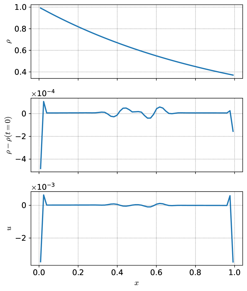
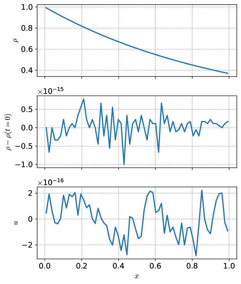
To test the method, I explore an isothermal hydrostatic atmosphere, with base density of $1$, pressure of $1$, and $g=-1$ in a domain $[0,1]$ (in code units). The initial atmosphere is constructed by first integrating from the lower boundary to the first cell center, and then differencing HSE as:

$$p_{i+1}=p_{i}+\frac{1}{2}\Delta x(\rho_{i}+\rho_{i+1})g$$ (37)

with an isothermal ideal gas. This is run for a time of 0.5 using PPMpy, with reflecting boundaries, which work well when the reconstruction is done with the perturbational pressure. Figure 1 shows the atmosphere with both the standard PPM reconstruction and this well-balanced method and demonstrates that with the well-balanced approach, the velocity is roundoff-level throughout the atmosphere.

The work at Stony Brook was supported by DOE/Office of Nuclear Physics grant DE-FG02-87ER40317.

References

  • Almgren et al. (2020) Almgren, A., Sazo, M. B., Bell, J., et al. 2020, Journal of Open Source Software, 5, 2513, doi: 10.21105/joss.02513
  • Colella & Woodward (1984) Colella, P., & Woodward, P. R. 1984, J. Comput. Phys., 54, 174, doi: 10.1016/0021-9991(84)90143-8
  • Hunter (2007) Hunter, J. D. 2007, Comput. Sci. Eng., 9, 90, doi: 10.1109/mcse.2007.55
  • Käppeli (2022) Käppeli, R. 2022, Living Reviews in Computational Astrophysics, 8, 2, doi: 10.1007/s41115-022-00014-6
  • Käppeli & Mishra (2016) Käppeli, R., & Mishra, S. 2016, A&A, 587, A94, doi: 10.1051/0004-6361/201527815
  • van der Walt et al. (2011) van der Walt, S., Colbert, S. C., & Varoquaux, G. 2011, Comput. Sci. Eng., 13, 22, doi: 10.1109/mcse.2011.37
  • Zingale (2024) Zingale, M. 2024, python-hydro/ppmpy: PPMpy 1.0.2, 1.0.2, Zenodo, doi: 10.5281/zenodo.13367094
  • Zingale et al. (2002) Zingale, M., Dursi, L. J., ZuHone, J., et al. 2002, Astrophysical Journal Supplement Series, The, 143, 539, doi: 10.1086/342754