Aspects of holographic Langevin diffusion in the presence of anisotropic magnetic field
Abstract
We revisit the holographic Langevin diffusion coefficients of a heavy quark, when travelling through a strongly coupled anisotropic plasma in the presence of magnetic field . The Langevin diffusion coefficients are calculated within the membrane paradigm in the magnetic branes model which has been extensively studied to investigate the magnetic effects on various observables in strongly coupled QCD scenarios by holography. In addition to confirming some conventional conclusions, we also find several new interesting features among the five Langevin diffusion coefficients in the magnetic anisotropic plasma. It is observed that the transverse Langevin diffusion coefficients depend more on the direction of motion rather than the directions of momentum diffusion at the ultra-fast limit, while one would find an opposite conclusion when the moving speed is sufficiently low. For the Longitudinal Langevin diffusion coefficient, we find that motion perpendicular to affects the Langevin coefficients stronger at any fixed velocity. We should also emphasize that all five Langevin coefficients are becoming larger with increasing velocity. We find that the universal relation in the isotropic background, is broken in a different new case that a quark moving paralleled to . This is one more particular example where the violation of the universal relation occurs for the anisotropic background. Further, we find the critical velocity of the violation will become larger with increasing .
I Introduction
A strong magnetic field is produced in heavy ion collisions (HICs) experiments at the Relativistic Heavy Ion Collider (RHIC) around and the Large Hadron Collider (LHC) up to Skokov et al. (2009); Deng and Huang (2012); Bloczynski et al. (2013); Tuchin (2013); Bali et al. (2012), which has attracted much attention to study the influences on properties of the quark gluon plasma (QGP) from the magnetic field. It’s also known the existence of even stronger magnetic fields in the interior of the dense neutron stars Duncan and Thompson (1992) and early stages of the Universe Vachaspati (1991); Grasso and Rubinstein (2001). In weakly coupled quantum chromodynamics (QCD) theory, the influences from the strong magnetic field to dynamic heavy quark has been studied at the Lowest-Landau-Level approximation, which for a thermal medium suggests the regime Fukushima et al. (2016); Kurian et al. (2019); Sadofyev and Yin (2016); Zhang et al. (2021); Bandyopadhyay et al. (2022).
The AdS/CFT correspondence Maldacena (1998); Witten (1998a); Gubser et al. (1998) is one of the very promising approaches to deal with these problems in QCD at strong couple scenario where can’t be perturbatively handled properly Witten (1998b); Aharony et al. (2000). On gravity side, the heavy quark diffusion in a strong coupled plasma can be understood as the fluctuation correlations of the trailing string. The studying of the stochastic nature of a heavy quark in a holography was proposed by Gubser (2008); Casalderrey-Solana and Teaney (2007). Soon the stochastic motion is formulated as a Langevin process de Boer et al. (2009); Son and Teaney (2009). Since the heavy quarks in HICs experiments are relativistic in many cases, the relativistic Langevin evolution are studied in Giecold et al. (2009) and in non-conformal frameworks in Gursoy et al. (2010); Kiritsis et al. (2012) for the multiple scales of QCD. The effect of the magnetic field directly on the heavy quark moving was studied in Matsuo et al. (2006); Kiritsis and Pavlopoulos (2012), which ignores the effect of the magnetic field on the plasma. It is studied that the heavy quark moving in magnetized plasma with ( is Lorentz factor and is heavy quark mass), at strong magnetic field limit Mamo (2016); Li et al. (2016). Other aspects of influences from magnetic field to heavy quark with holography Zhu et al. (2022); Zhang and Ma (2018); Zhang et al. (2018); Zhang (2019); Zhu et al. (2019, 2020); Zhou et al. (2020); Chen et al. (2018); He et al. (2013); Dudal and Mertens (2018); Giataganas (2018); Iwasaki et al. (2021); Chakrabortty et al. (2014); Rougemont (2020); Fischler et al. (2014); Rougemont et al. (2015); Bu et al. (2022); Bu and Zhang (2021).
An universal inequality relation, , has been found in the generic isotropic background with AdS/CFT correspondence Gursoy et al. (2010); Pourhassan et al. (2017). A way to violate this relation is to consider the Brownian motion in anisotropic background. And the fact that the transverse LGV-coefficient may be larger than a specific longitudinal LGV-coefficient, is found in both JW and MT spatial anisotropic background in Giataganas and Soltanpanahi (2014a). Due to the rapid expansion along the beam direction, the QGP experiences an anisotropic phase both in momentum and coordinate space before the system reaches the isotropic phase in a short period of time. And the strong magnetic field is another important source of anisotropy, and it is interesting to study its influence on heavy quark diffusion at HICs. To be specific we want to investigate how the anisotropy induced by an uniform magnetic field affects the both longitudinal and transverse LGV-coefficients.
In this work, we will study LGV-coefficients with the magnetic branes model to present our findings. Besides the confirmation of some conventional conclusions found before, we will conduct an in-depth investigation about heavy quark diffusion with LGV-coefficients in the presence of a uniform magnetic field with holography. We also want to study the heavy quark diffusion in an anisotropic background with a uniform magnetic field . The relations between LGV-coefficients in an anisotropic background also is an important motivation for this work. Also, we hope our study could shed light on to transport and hydrodynamic Monte Carlo simulation of HICs.
This paper is organized as follows. In the next section section II, we will review the magnetic branes model and also the main procedures to deduce LGV-coefficients within the membrane paradigm. We discuss all five LGV-coefficients and study the influences to relativistic LGV-coefficients from a uniform magnetic field at the different setups in section III. In section IV, we give parameterized expressions to all five LGV-coefficients in the case of a strong magnetic field limit . The last part V is devoted to a short summary.
II The setups
The top-down magnetic branes model is dual to a deformed strong coupled SYM theory with a constant magnetic field. The bulk action is a uniform Maxwell field coupled to 5 dimension Einstein gravity with a negative cosmological constant D’Hoker and Kraus (2009),
| (1) |
where is the 5 dimension gravitational constant and stands for the Maxwell field strength 2-form, the radius of the spacetime is set to unity for the rest of the paper. contains the Chern-Simons terms, Gibbons-Hawking terms and other contributions necessary for a well posed variational principle. There is no sense of confinement for the nonexistence of dilaton field.
Following the general ansatz in D’Hoker and Kraus (2009), the anisotropic magnetic branes background with a uniform magnetic field is given as
| (2) |
for metric. And for field strength , one has
| (3) |
with constant for the magnetic field strength along axis- direction. The horizon is located at and the boundary is located at . The three functions , , and are obtained by solving the equations of motion.
Maxwell’s equations following from (1) are automatically satisfied by the ansatz (2), while the set of linearly independent components read
| (4) |
| (5) |
| (6) |
| (7) |
A charged system will undergo a dimensional reduction in the presence of strong fields due to the projection towards the lowest Landau level Shovkovy (2013); Gusynin et al. (1996). The magnetic branes solution must satisfy two sets of boundary conditions, which corresponds to a holographic renormalization group flow interpolating between a near horizon solution and a near boundary asymptotic solution at . On the one hand, the geometry (2) in IR should reduce to a black hole Banados et al. (1992) times a two dimensional torus in the spatial directions transverse to the magnetic field. The exact analytical solution near the horizon () was found as
| (8) |
with and refers to the the black hole radius. On the other hand, there should be a near boundary asymptotic solution at ,
| (9) |
for one we must recover the dynamics of SYM without the influence of the magnetic field at UV.
Following the procedure mentioned in D’Hoker and Kraus (2009), here one constructs a numerical solution that interpolates between the near horizon and asymptotic in the boundary. To fix the horizon at , one use rescaled coordinates so that also give
| (10) |
With a rescaled , one take
| (11) |
which sets the temperature to a fixed value and leave as the free parameter. Further one take
| (12) |
with the help of rescaled , , .
With these conditions, (4) and (6) give us the initial data
| (13) |
where stands for the value of the magnetic field in the rescaled coordinates.
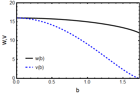
Integrating the ODE out from to a large value of , one find geometry will have the asymptotic behavior at ,
| (14) |
where and are parameters which can be determined numerically. We plot two key coefficients and in Fig.(1) as a function of , which is match to Fig.(1) in Critelli et al. (2014).
Since the solution should have an asymptotic at the UV, one can introduce coordinate
| (15) |
then he full bulk metric (2) after these rescalings reads
| (16) |
One can obtain the thermodynamics of the gauge theory from (16). And the rescaled magnetic field is related to the bulk magnetic field by
| (17) |
Since the geometry has to be asymptotic at UV, the first equation in (13) imply . The physically observable magnetic field at the boundary , as argued in D’Hoker and Kraus (2009) by comparing the Chern-Simons term in (2) with the SYM chiral anomaly. By using the fact that any physical quantity in this model should depend on the dimensionless quantity, ratio , one fixs the temperature at thus compute
| (18) |
Next, we compute the LGV-coefficients of a heavy quark in a uniform magnetic field induced anisotropy medium by following the author of Gursoy et al. (2010); Giataganas and Soltanpanahi (2014a); Finazzo et al. (2016). We consider a general diagonal metric in radial coordinates,
| (19) |
where the boundary is . For simplicity, one set similar to magnetic branes geometry (2). Here, we consider a quark moving at direction and transverse to direction , and calculate the LGV-coefficients transverse to direction and along direction respectively.
Holographically, the moving heavy quark of infinite mass on the boundary CFT correspond to the endpoint of the trailing string. The string dynamics are captured by the Nambu-Goto action
| (20) |
where is the induced metric, and and are the branes metric and target space coordinates.
A moving heavy quark with a constant velocity has the usual parametrization
| (21) |
where is the profile of the string in the bulk. Then it’s is deduced the world-sheet metric
| (22) |
One can find the critical point from , which means we find by solve the
| (23) |
proportional to radial conjugate momentum.
One find the effective temperature of the world-sheet horizon by diagonal world-sheet metric.
| (24) |
Further is the diagonal induced world-sheet metric given
| (25) | |||
Following the usual procedure, the effective temperature reads
| (26) | ||||
Considering the fluctuation in classical trailing string, one has
| (27) |
where the fluctuation of the form along longitudinal and transverse direction of . The action capture fluctuations around the trailing string reads
| (28) |
Taking advantage of the membrane paradigm Iqbal and Liu (2009), one can directly reads LGV-coefficients without solving motion equation,
| (29) |
and
| (30) |
In the case of magnetic black branes, one can directly reads from the metric (16) as
| (31) | |||
| (32) | |||
| (33) | |||
| (34) |
When the quark moving along , one have a longitudinal LGV-coefficients and one transverse LGV-coefficient . Inserting (33) into (26), one have effective temperature
| (35) |
With and , one the expressions into (30) and (29), then get
| (36) |
When the quark moving transverse to , one also have a longitudinal LGV-coefficients but two transverse LGV-coefficient and , for the anisotropy in plane transverse to motion. We denote as the transverse LGV-coefficient when quark moving perpendicular to the direction of and diffusion paralleled to the direction of motion. We also denote as the transverse LGV-coefficient when moving and diffusion direction perpendicular to the direction of . Inserting (32) into (26), we have effective temperature
| (37) |
With and , one inserts the expressions into (30) and (29), then get
| (38) |
With and , one the inserts expressions into (29), then get
| (39) |
III Numeric Results
III.1 Directions dependence
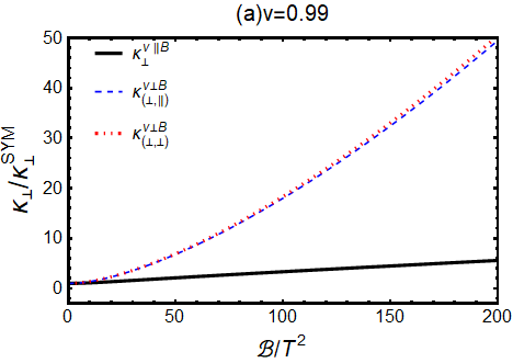
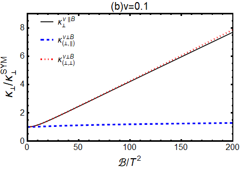
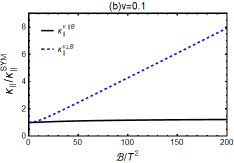
Initially, in this subsection, we will examine two extreme cases to study the relations between different LGV-coefficients in all scale with , for which is the only dimensionless parameter in this model. The numerical results of transverse LGV-coefficients and longitudinal LGV-coefficients as a function of magnetic field are displayed in Fig. 2 and Fig.3, normalized by the conform limit given in (40). Fig. 2 show transverse LGV-coefficients , and , while Fig. 3 show longitudinal LGV-coefficients and .
When moving at the ultra fast limit, as shown in plot (a) in Fig. 2, the transverse LGV-coefficients of quark has a relation reads , which means the transverse LGV-coefficients of quark mostly depending on the direction of moving but not the direction of transverse momentum diffusion when the moving velocity approaching to light speed. It also means that the anisotropy in plane contributes little to the strength of transverse LGV-coefficients when moving in ultra-fast limit. But when the moving velocity is sufficiently small, is taken for example, one will find an opposite conclusion that the transverse LGV-coefficients of quark depend more on the direction of transverse momentum diffusion rather than the direction of moving.
As for the longitudinal LGV-coefficients shown in Fig. 3, we find that at both ultra fast limit and a fixed sufficiently small speed. And moving perpendicular to direction affects the longitudinal LGV-coefficients stronger compared to motion along direction. So we conclude that the transverse LGV-coefficients may be more sensitive to the anisotropic magnetic background rather than the Longitudinal LGV-coefficients .
By comparing transverse LGV-coefficients in Fig. 2 and the longitudinal LGV-coefficients in Fig. 3, we find that the transverse LGV-coefficients may be more sensitive to the anisotropic magnetic background rather than the Longitudinal LGV-coefficients. Finally, the LGV-coefficient always enhances with increasing magnetic field in all cases for both transverse and longitudinal LGV-coefficients.
III.2 Dynamic properties
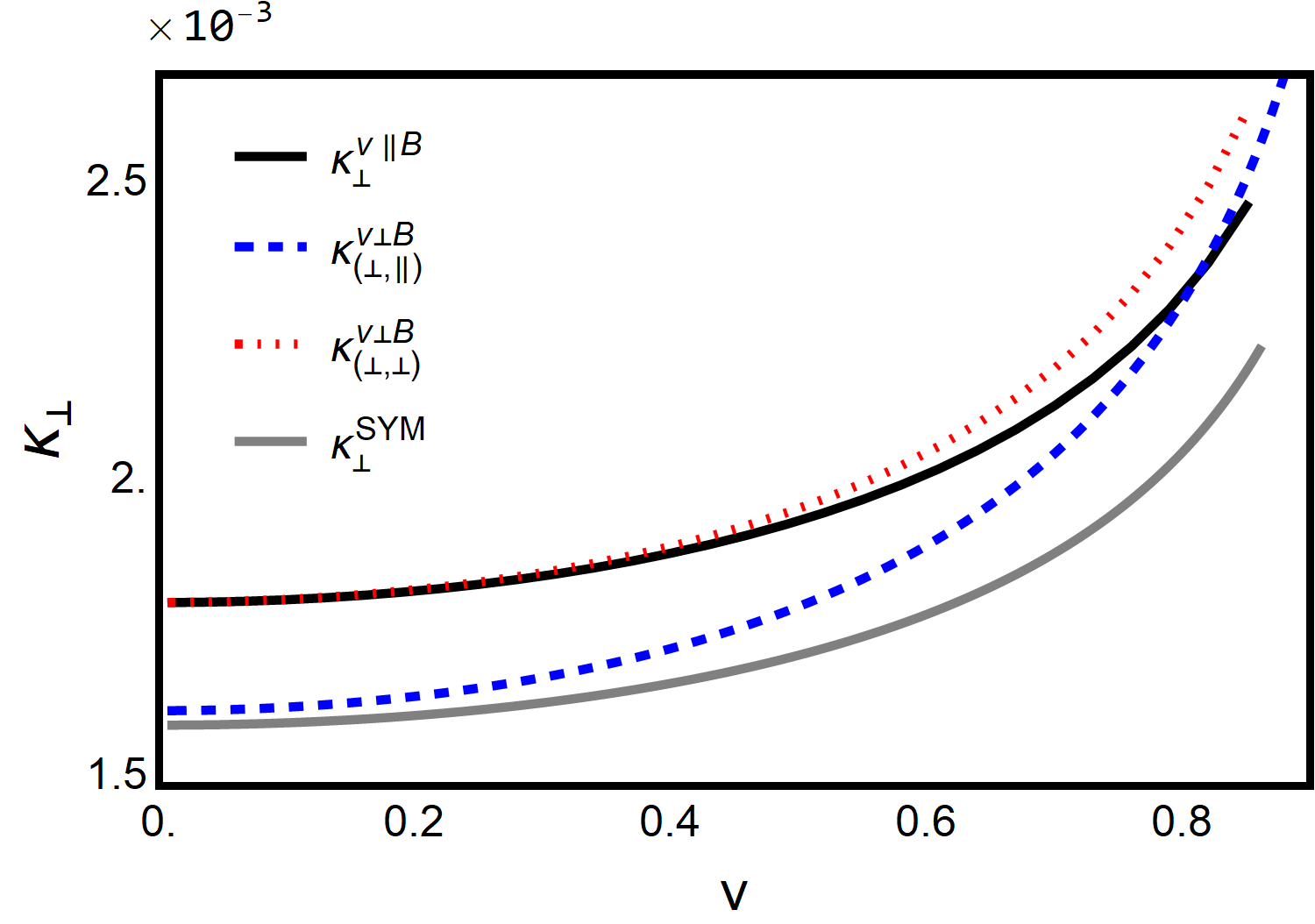
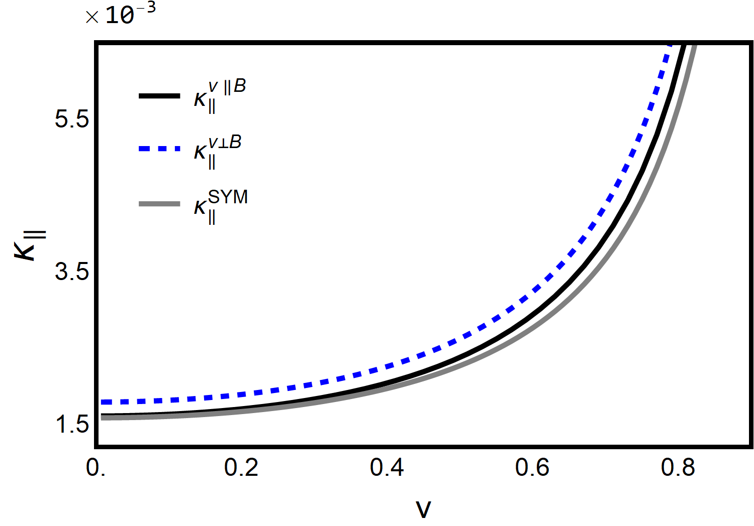
We further examine the impact of moving velocity on both transverse and longitudinal LGV-coefficients. In Fig. 4, we plot the LGV-coefficients as a function of quark moving velocity , accompanied by the corresponding results in conformal limit at (40). It demonstrates that the increasing moving velocity enhances the LGV-coefficients in all cases we mentioned in this anisotropic magnetic background, which is very similar to the results in the conformal limit. This conclusion is also similar to the outcomes in spatial anisotropic case in Giataganas and Soltanpanahi (2014b).
Unlike the two extreme cases with fixed speeds in III.1, we can study the same question with varying moving speeds. It is found that, at a sufficiently small moving speed, the momentum broadening of a heavy quark depends more on the direction of momentum diffusion rather than the direction of moving with both in the upper panel and in the lower panel of Fig. (4).
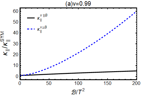
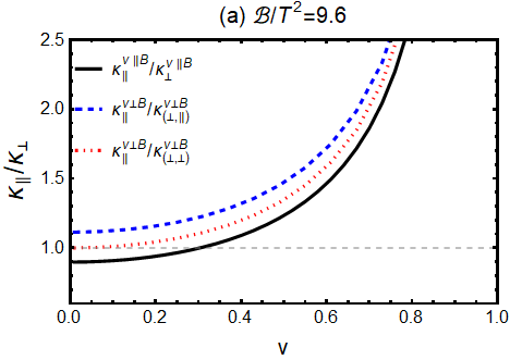
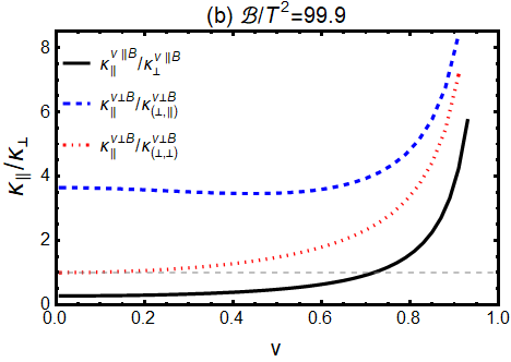
III.3 Violations of the longitudinal to transverse LGV-coefficient ratios
With both transverse and longitudinal LGV-coefficients, it is possible to take an investigation into the universal equation Gursoy et al. (2010) in this top-down magnetic branes model, where anisotropy is introduced by a uniform constant magnetic field. Fig. 5 presents numerical results of the ratios of longitudinal over transverse LGV-coefficients, , as a function of quark moving velocity . One can find that at sufficient low speed, which violate the universal equation found in isotropic background. In our study, the violation occurs at a sufficiently low speed only when moving parallel to the direction of a magnetic field. This is one more particular example where the violation of the universal relation compared to the spatial anisotropic background found in Giataganas and Soltanpanahi (2014a).
By comparing plot (a) and plot (b) in Fig. 5, one can further take an investigation the influences on the violation from increasing magnetic field strength . We find the critical velocity of violation become larger with increasing magnetic strength , then we can conclude that the relationship, , will eventually be violated as long as the magnetic field is strong enough in this magnetic anisotropic plasma. Even more one can conclude from our numeric results that this violation should exist in the diffusion of heavy quark jets, where a strong magnetic field is created at HICs.
IV Near horizons analytical limit
One has a special geometry in the case of the strong magnetic field , which is a product of 3 dimension and trivial flat 2 dimension as mentioned in section II. The exact solution near the horizon (), which denotes the product of a black hole times a two dimensional torus , was found as
| (41) |
with and referring to the the black hole radius. The horizon is located at and the boundary located at . The Hawking temperature of the black hole .
One has
| (42) |
By repeating the procedure in section II, one has critical point when a heavy quark moving paralleled to magnetic field , as
| (43) |
The effective temperature of 2 dimensional black hole of a quark feel denoted as when quark moving along and transverse to magnetic field ,
| (44) |
Asserting (42) to (26), (30) and (29), one get longitudinal and perpendicular LGV-coefficients as
| (45) |
and
| (46) |
Similar to the parallel case, computations of the LGV-coefficients for a quark moving perpendicular to a magnetic field can be done. The critical point is at
| (47) |
The effective temperature temperature reads
| (48) |
The perpendicular and longitudinal LGV-coefficients reads
| (49) |
and
| (50) |
and
| (51) |
It should be mentioned that the perpendicular LGV-coefficients (46), (50) and (51) have been calculated to compute jet quenching parameters in Li et al. (2016). In present study, we recompute these quantities including the two additional longitudinal LGV-coefficients (45) and (49) for completeness. In the case of the strong magnetic fie , the final results of (49), (50) and (51) have ignore the in our calculation. We recommend Li et al. (2016) for discussion about . The longitudinal LGV-coefficients is independent of and similar to weak coupling results of introduced in Fukushima et al. (2016). However, it’s demonstrated from (51) that depends on as at leading order.
V Conclusion
The study of jet quenching properties as functions of parameters such as the temperature, chemical potential, anisotropy or magnetic field strength are all of great relevance for the characterization and understanding of the QGP. In the present work, we take an investigation on relativistic heavy quark diffusion in strongly coupled anisotropic plasma with uniform magnetic field. It should be noticed that we present several new dynamic properties on Langevin diffusion of a heavy quark in this work.
With the membrane paradigm approach, we calculate five LGV-coefficients in a top-down magnetic branes model. With increasing magnetic field , it is observed that all LGV-coefficients become larger with increasing anisotropic magnetic field which also has been observed in magnetized gravity-dilaton system Rougemont et al. (2015). We also find all the LGV-coefficients becoming larger with increasing speed, which is similar to the behaviors in the case of both pure SYM theory Gubser (2008); Casalderrey-Solana and Teaney (2007) and axion-driven anisotropy theroy Giataganas and Soltanpanahi (2014b).
Comparing LGV-coefficients when quark motions in different direction, we find several new interesting features. It is observed that the transverse LGV-coefficients depend more on the direction of motion than the direction of diffusion at the ultra-fast limit, while one would find an opposite conclusion when it comes to a lower moving speed. For Longitudinal LGV-coefficients, we find that motion perpendicular to affects the LGV-coefficients stronger at a fixed velocity.
In isotropic case, a universal relation has been found. It is also found the universal property proved are broken in the anisotropic case. We find that the universal relation is broken in a new case that a quark moving paralleled to , which is different from the fraction found in spatial anisotropy case Giataganas and Soltanpanahi (2014a). We also find the critical velocity of the violation will become larger with increasing .
We also calculate all five LGV-coefficients for completeness in BTZ background corresponding to strong magnetic field limit .
ACKNOWLEDGMENTS
This research is supported by the Guangdong Major Project of Basic and Applied Basic Research No. 2020B0301030008, and Natural Science Foundation of China with Project Nos. 11935007.
References
- Skokov et al. (2009) V. Skokov, A. Y. Illarionov, and V. Toneev, Int. J. Mod. Phys. A 24, 5925 (2009), arXiv:0907.1396 [nucl-th] .
- Deng and Huang (2012) W.-T. Deng and X.-G. Huang, Phys. Rev. C 85, 044907 (2012), arXiv:1201.5108 [nucl-th] .
- Bloczynski et al. (2013) J. Bloczynski, X.-G. Huang, X. Zhang, and J. Liao, Phys. Lett. B 718, 1529 (2013), arXiv:1209.6594 [nucl-th] .
- Tuchin (2013) K. Tuchin, Adv. High Energy Phys. 2013, 490495 (2013), arXiv:1301.0099 [hep-ph] .
- Bali et al. (2012) G. S. Bali, F. Bruckmann, G. Endrodi, Z. Fodor, S. D. Katz, S. Krieg, A. Schafer, and K. K. Szabo, JHEP 02, 044 (2012), arXiv:1111.4956 [hep-lat] .
- Duncan and Thompson (1992) R. C. Duncan and C. Thompson, Astrophys. J. Lett. 392, L9 (1992).
- Vachaspati (1991) T. Vachaspati, Phys. Lett. B 265, 258 (1991).
- Grasso and Rubinstein (2001) D. Grasso and H. R. Rubinstein, Phys. Rept. 348, 163 (2001), arXiv:astro-ph/0009061 .
- Fukushima et al. (2016) K. Fukushima, K. Hattori, H.-U. Yee, and Y. Yin, Phys. Rev. D 93, 074028 (2016), arXiv:1512.03689 [hep-ph] .
- Kurian et al. (2019) M. Kurian, S. K. Das, and V. Chandra, Phys. Rev. D 100, 074003 (2019), arXiv:1907.09556 [nucl-th] .
- Sadofyev and Yin (2016) A. V. Sadofyev and Y. Yin, Phys. Rev. D 93, 125026 (2016), arXiv:1511.08794 [hep-th] .
- Zhang et al. (2021) H.-X. Zhang, J.-W. Kang, and B.-W. Zhang, Eur. Phys. J. C 81, 623 (2021), arXiv:2004.08767 [hep-ph] .
- Bandyopadhyay et al. (2022) A. Bandyopadhyay, J. Liao, and H. Xing, Phys. Rev. D 105, 114049 (2022), arXiv:2105.02167 [hep-ph] .
- Maldacena (1998) J. M. Maldacena, Adv. Theor. Math. Phys. 2, 231 (1998), arXiv:hep-th/9711200 .
- Witten (1998a) E. Witten, Adv. Theor. Math. Phys. 2, 253 (1998a), arXiv:hep-th/9802150 .
- Gubser et al. (1998) S. S. Gubser, I. R. Klebanov, and A. M. Polyakov, Phys. Lett. B 428, 105 (1998), arXiv:hep-th/9802109 .
- Witten (1998b) E. Witten, Adv. Theor. Math. Phys. 2, 505 (1998b), arXiv:hep-th/9803131 .
- Aharony et al. (2000) O. Aharony, S. S. Gubser, J. M. Maldacena, H. Ooguri, and Y. Oz, Phys. Rept. 323, 183 (2000), arXiv:hep-th/9905111 .
- Gubser (2008) S. S. Gubser, Nucl. Phys. B 790, 175 (2008), arXiv:hep-th/0612143 .
- Casalderrey-Solana and Teaney (2007) J. Casalderrey-Solana and D. Teaney, JHEP 04, 039 (2007), arXiv:hep-th/0701123 .
- de Boer et al. (2009) J. de Boer, V. E. Hubeny, M. Rangamani, and M. Shigemori, JHEP 07, 094 (2009), arXiv:0812.5112 [hep-th] .
- Son and Teaney (2009) D. T. Son and D. Teaney, JHEP 07, 021 (2009), arXiv:0901.2338 [hep-th] .
- Giecold et al. (2009) G. C. Giecold, E. Iancu, and A. H. Mueller, JHEP 07, 033 (2009), arXiv:0903.1840 [hep-th] .
- Gursoy et al. (2010) U. Gursoy, E. Kiritsis, L. Mazzanti, and F. Nitti, JHEP 12, 088 (2010), arXiv:1006.3261 [hep-th] .
- Kiritsis et al. (2012) E. Kiritsis, L. Mazzanti, and F. Nitti, J. Phys. G 39, 054003 (2012), arXiv:1111.1008 [hep-th] .
- Matsuo et al. (2006) T. Matsuo, D. Tomino, and W.-Y. Wen, JHEP 10, 055 (2006), arXiv:hep-th/0607178 .
- Kiritsis and Pavlopoulos (2012) E. Kiritsis and G. Pavlopoulos, JHEP 04, 096 (2012), arXiv:1111.0314 [hep-th] .
- Mamo (2016) K. A. Mamo, Phys. Rev. D 94, 041901 (2016), arXiv:1606.01598 [hep-th] .
- Li et al. (2016) S. Li, K. A. Mamo, and H.-U. Yee, Phys. Rev. D 94, 085016 (2016), arXiv:1605.00188 [hep-ph] .
- Zhu et al. (2022) Z.-R. Zhu, J. Chen, and D. Hou, Eur. Phys. J. A 58, 104 (2022), arXiv:2109.09933 [hep-ph] .
- Zhang and Ma (2018) Z.-q. Zhang and K. Ma, Eur. Phys. J. C 78, 532 (2018).
- Zhang et al. (2018) Z.-q. Zhang, K. Ma, and D.-f. Hou, J. Phys. G 45, 025003 (2018), arXiv:1802.01912 [hep-th] .
- Zhang (2019) Z.-q. Zhang, Phys. Lett. B 793, 308 (2019).
- Zhu et al. (2019) Z.-R. Zhu, S.-Q. Feng, Y.-F. Shi, and Y. Zhong, Phys. Rev. D 99, 126001 (2019), arXiv:1901.09304 [hep-ph] .
- Zhu et al. (2020) Z.-R. Zhu, D.-f. Hou, and X. Chen, Eur. Phys. J. C 80, 550 (2020), arXiv:1912.05806 [hep-ph] .
- Zhou et al. (2020) J. Zhou, X. Chen, Y.-Q. Zhao, and J. Ping, Phys. Rev. D 102, 086020 (2020), arXiv:2006.09062 [hep-ph] .
- Chen et al. (2018) X. Chen, S.-Q. Feng, Y.-F. Shi, and Y. Zhong, Phys. Rev. D 97, 066015 (2018), arXiv:1710.00465 [hep-ph] .
- He et al. (2013) S. He, S.-Y. Wu, Y. Yang, and P.-H. Yuan, JHEP 04, 093 (2013), arXiv:1301.0385 [hep-th] .
- Dudal and Mertens (2018) D. Dudal and T. G. Mertens, Phys. Rev. D 97, 054035 (2018), arXiv:1802.02805 [hep-th] .
- Giataganas (2018) D. Giataganas, PoS CORFU2017, 032 (2018), arXiv:1805.09011 [hep-th] .
- Iwasaki et al. (2021) S. Iwasaki, M. Oka, and K. Suzuki, Eur. Phys. J. A 57, 222 (2021), arXiv:2104.13990 [hep-ph] .
- Chakrabortty et al. (2014) S. Chakrabortty, S. Chakraborty, and N. Haque, Phys. Rev. D 89, 066013 (2014), arXiv:1311.5023 [hep-th] .
- Rougemont (2020) R. Rougemont, Phys. Rev. D 102, 034009 (2020), arXiv:2002.06725 [hep-ph] .
- Fischler et al. (2014) W. Fischler, P. H. Nguyen, J. F. Pedraza, and W. Tangarife, JHEP 08, 028 (2014), arXiv:1404.0347 [hep-th] .
- Rougemont et al. (2015) R. Rougemont, R. Critelli, and J. Noronha, Phys. Rev. D 91, 066001 (2015), arXiv:1409.0556 [hep-th] .
- Bu et al. (2022) Y. Bu, B. Zhang, and J. Zhang, Phys. Rev. D 106, 086014 (2022), arXiv:2210.02274 [hep-th] .
- Bu and Zhang (2021) Y. Bu and B. Zhang, Phys. Rev. D 104, 086002 (2021), arXiv:2108.10060 [hep-th] .
- Pourhassan et al. (2017) B. Pourhassan, M. Karimi, and S. Mojarrad, Acta Phys. Polon. B 48, 1507 (2017), arXiv:1709.06846 [hep-th] .
- Giataganas and Soltanpanahi (2014a) D. Giataganas and H. Soltanpanahi, Phys. Rev. D 89, 026011 (2014a), arXiv:1310.6725 [hep-th] .
- D’Hoker and Kraus (2009) E. D’Hoker and P. Kraus, JHEP 10, 088 (2009), arXiv:0908.3875 [hep-th] .
- Shovkovy (2013) I. A. Shovkovy, Lect. Notes Phys. 871, 13 (2013), arXiv:1207.5081 [hep-ph] .
- Gusynin et al. (1996) V. P. Gusynin, V. A. Miransky, and I. A. Shovkovy, Nucl. Phys. B 462, 249 (1996), arXiv:hep-ph/9509320 .
- Banados et al. (1992) M. Banados, C. Teitelboim, and J. Zanelli, Phys. Rev. Lett. 69, 1849 (1992), arXiv:hep-th/9204099 .
- Critelli et al. (2014) R. Critelli, S. I. Finazzo, M. Zaniboni, and J. Noronha, Phys. Rev. D 90, 066006 (2014), arXiv:1406.6019 [hep-th] .
- Finazzo et al. (2016) S. I. Finazzo, R. Critelli, R. Rougemont, and J. Noronha, Phys. Rev. D 94, 054020 (2016), [Erratum: Phys.Rev.D 96, 019903 (2017)], arXiv:1605.06061 [hep-ph] .
- Iqbal and Liu (2009) N. Iqbal and H. Liu, Phys. Rev. D 79, 025023 (2009), arXiv:0809.3808 [hep-th] .
- Giataganas and Soltanpanahi (2014b) D. Giataganas and H. Soltanpanahi, JHEP 06, 047 (2014b), arXiv:1312.7474 [hep-th] .