Nonlinear Modified PageRank Problem for Local Graph Partitioning

Abstract

A nonlinear generalisation of the PageRank problem involving the Moore-Penrose inverse of the incidence matrix is developed for local graph partitioning purposes. The Levenberg-Marquardt method with a full rank Jacobian variant provides a strategy for obtaining a numerical solution to the generalised problem. Sets of vertices are formed according to the ranking supplied by the solution, and a conductance criterion decides upon the set that best represents the cluster around a starting vertex. Experiments on both synthetic and real-world inspired graphs demonstrate the capability of the approach to not only produce low conductance sets, but to also recover local clusters with an accuracy that consistently surpasses state-of-the-art algorithms.

05C50, 65K05, 90C35, 90C90

1 Introduction

Graphs are a particularly convenient apparatus for representing associations and their value between objects. It is the very abstraction inherent in the definition of a graph that makes them so widely applicable. Vertices can be any kind of object (images [10], geographical locations [28], etc.), and this has no bearing on the graph at all. Furthermore, no restrictions are put on the number of edges, that is, associations, between any one vertex and the others.

A graph may well exhibit a granular structure. Vertices that share a common property can be uncovered by a process called clustering. The resulting distinct groupings of vertices are referred to as communities or clusters. For example, if all associations are equally valuable, then it may be that communities are distinguished by the relatively high number of intra-community edges compared to the inter-community number of edges.

Spectral clustering is a prominent algorithm that casts clustering as a graph partitioning problem. Clusters are determined through an analysis of the combinatorial Laplacian matrix eigenvectors [24, 36]. A generalisation of spectral clustering utilising the $p$-Laplacian [1, 35] was pursued in [5]. Improved clustering assignments were demonstrated in the bi-partitioning case. Recursive extension was, however, used for obtaining a greater number of clusters. Direct multiway approaches include approximating the $p$-orthogonality constraint [22, 27], the effective $p$-resistance [33], and exploiting concepts from total variation used commonly in image processing [4].

When only a single cluster around a vertex or vertices is of interest, then an alternative strategy can be employed. Local clustering, as the name suggests, seeks to leverage local structure and information to identify a cluster. This has the potential to improve algorithmic run-time by avoiding computations over the entirety of a graph.

Treatment of clustering as a partitioning problem carries over into local clustering. A cut can be found using a variation of the PageRank problem [2]. Since a PageRank vector provides a ranking of vertices (refer to [19] for information on functional rankings), sets of vertices can then be assembled according to their order and interrogated to reveal a cut. Just as with spectral clustering, the $p$-norm has found its way into local clustering algorithms. There is the nonlinear $p$-norm cut algorithm [21], and an algorithm based on the idea of diffusion with $p$-norm network flow [11].

This work takes the system of linear equations that forms the PageRank problem as the starting point in the construction of a local clustering algorithm. Only clusters around a single vertex are considered. A modification to the PageRank problem is studied in Section 3. This is followed with the theoretical motivation for a nonlinear generalisation (that is, of the modified PageRank problem) involving the $p$-norm in Section 4. The Moore-Penrose inverse of the incidence matrix plays a very important role in the generalisation. It is shown in Section 4 that the generalisation can reduce to a system of linear equations closely resembling the modified PageRank problem. However, this is dependent on a number of conditions, with a major one being that the number of vertices approaches infinity. Additionally, an insight into the effect of the generalised problem on the cluster criterion based on an infinitesimal perturbation argument can be found in Section 4. The Levenberg-Marquardt method with a full rank Jacobian variant is presented in Section 5 for obtaining a numerical solution to the generalised problem.

The next section is a short compendium of theories required for the development of the generalised problem and the identification of a cluster. Section 6 highlights the capability of the proposed algorithm on a number of synthetic and real-world inspired graphs. The algorithm performs strongly on a consistent basis, achieving results better than state-of-the-art algorithms.

2 Preliminaries

2.1 Notions of graph theory

A graph $\mathcal{G}=(\mathcal{V},\mathcal{E})$ consists of a finite set $\mathcal{V}$ of vertices and a set of unordered non-repeated pairs of distinct elements of $\mathcal{V}$ called edges, $\mathcal{E}\subseteq\mathcal{V}\times\mathcal{V}$. Any two vertices $u,v\in\mathcal{V}$ are said to be adjacent or neighbours if they form an edge $e=\{u,v\}$ of $\mathcal{E}$. Their relationship is indicated by $u\sim v$. By definition, there can be no loops, i.e., $\{v,v\}\notin\mathcal{E}$, and only one edge can ever join two vertices. Such a graph is often described as being simple.

If a path exists between every pair of vertices $u$ and $v$ in $\mathcal{G}$, that is, a sequence of vertices $u=u_{1},u_{2},\ldots,u_{n},u_{n+1}=v$ with $e_{i}=\{u_{i},u_{i+1}\}\in\mathcal{E}$ for $i=1,2,\ldots,n$, then the graph is referred to as connected.

A graph $\mathcal{F}=(\dot{\mathcal{V}},\dot{\mathcal{E}})$ with $\dot{\mathcal{V}}\subseteq\mathcal{V}$ and $\dot{\mathcal{E}}\subseteq\mathcal{E}$ is said to be a subgraph of $\mathcal{G}$. Meanwhile, $\mathcal{G}$ becomes a host graph of $\mathcal{F}$. If $\mathcal{F}\neq\mathcal{G}$, then the subgraph is called proper. For $\mathcal{F}$ to be an induced subgraph, $\dot{\mathcal{E}}$ must contain all the edges of $\mathcal{E}$ required to maintain the adjacency relationships in host graph $\mathcal{G}$ between the vertices of $\dot{\mathcal{V}}$.

A weighted graph is a graph $\mathcal{G}=(\mathcal{V},\mathcal{E})$ with an associated weight function $w:\mathcal{V}\times\mathcal{V}\to[0,\infty)$, commonly expressed as the triple $\mathcal{G}=(\mathcal{V},\mathcal{E},w)$, satisfying $w(v,v)=0$ if $v\in\mathcal{V}$, $w(u,v)=w(v,u)$ if $u\sim v$, and $w(u,v)=0$ if and only if $u\not\sim v$. Furthermore, $w(u,v)>0$ for all $\{u,v\}\in\mathcal{E}$. Hereafter, only simple, connected and weighted graphs will be considered. A graph $\mathcal{G}$ should be read in this context.

Remark 2.1.

A weight function $w(u,v)=1$ for all $\{u,v\}\in\mathcal{E}$ represents the non-weighted graph equivalent.

Let $\mathcal{H}(\mathcal{V})$ denote the Hilbert space of real-valued functions defined on the vertices of a graph $\mathcal{G}$. Elements of $\mathcal{H}(\mathcal{V})$ assign a real-value, say $x(v)$, to each vertex $v\in\mathcal{V}$. The standard inner product $\langle x,y\rangle=\sum_{v\in V}x(v)y(v)$, where $x,y\in\mathcal{H}(\mathcal{V})$, will be assumed. For $x\in\mathcal{H}(\mathcal{V})$, the norm is then given by $\lVert x\rVert=\sqrt{\langle x,x\rangle}$. $x$ can be treated as the column vector $x=\left(x(v_{1}),x(v_{2}),\ldots,x(v_{|\mathcal{V}|})\right)^{\top}$ in $\mathbb{R}^{|\mathcal{V}|}$.

2.2 Conductance and sweep-cut

For a subset $\mathcal{S}$ of the vertices in a graph $\mathcal{G}$, i.e., $\mathcal{S}\subseteq\mathcal{V}$, the volume of $\mathcal{S}$ has the form

$$\text{vol}\,(\mathcal{S})=\sum_{v\in\mathcal{S}}d(v),$$

in which $d(v)$ stands for the (weighted) degree of vertex $v\in\mathcal{V}$:

$$d(v)=\sum_{u\sim v}w(u,v).$$

The complement of $\mathcal{S}$ is $\bar{\mathcal{S}}=\mathcal{V}\setminus\mathcal{S}$. An edge boundary $\partial(\mathcal{S})$ of $\mathcal{S}$ collects the edges with one vertex in $\mathcal{S}$ and the other in $\bar{\mathcal{S}}$, that is,

$$\partial(\mathcal{S})=\left\{\{u,v\}\in\mathcal{E}\mid u\in\mathcal{S}\mbox{ and }v\in\bar{\mathcal{S}}\right\}.$$

Conductance (or the Cheeger ratio) of $\mathcal{S}$ is defined to be

$$\Phi(\mathcal{S})=\frac{w\left(\partial(\mathcal{S})\right)}{\min\left(\text{vol}\,(\mathcal{S}),\text{vol}\,(\bar{\mathcal{S}})\right)},$$

where $w\left(\partial(\mathcal{S})\right)=\sum_{e\in\partial(\mathcal{S})}w(e)$.

A graph can be partitioned into two based on the conductance. This can be accomplished through a sweep over a vector $x\in\mathcal{H}(\mathcal{V})$ for cut (edges), $\partial(\mathcal{S})$, discovery. Suppose $v_{1},\ldots,v_{|\mathcal{V}|}$ is an ordering of vertices such that $x(v_{i})\geq x(v_{i+1})$ for $i=1,\ldots,|\mathcal{V}|-1$. What are known as sweep sets $\mathcal{S}_{j}=\{v_{1},\ldots,v_{j}\}$ for all $j\in\mathcal{N}=\{1,\ldots,|\mathcal{V}|-1\}$ can then be formed. It is the smallest conductance

$$\Phi(\mathcal{S}_{*})=\arg\,\min_{j\in\mathcal{N}}\,\Phi(\mathcal{S}_{j})$$

which provides the partition.

2.3 Matrix representation of graphs

Structural information of a graph $\mathcal{G}$ can be encoded in matrix form. Let $n=|\mathcal{V}|$ and $m=|\mathcal{E}|$. Connectivity between vertices is captured in the $n\times n$ symmetric adjacency matrix $A$, which has the entries

$$a_{ij}=\begin{cases}w\left(v_{i},v_{j}\right),&\mbox{ if }v_{i}\sim v_{j},\\ 0,&\mbox{ otherwise}.\end{cases}$$

The degree matrix $D$ is the diagonal matrix with $d_{ii}=\sum_{j=1}^{n}a_{ij}=d(v_{i})$ for $i=1,2,\ldots,n$ and $v_{i}\in V$. A (random walk) transition probability matrix can then be defined as $P=D^{-1}A$.

Edge-vertex connectivity features in the $m\times n$ incidence matrix $B$. For the sole purpose of the definition, an orientation on the graph is required. This entails the specification of an arbitrary but fixed order to the vertices of every edge in $\mathcal{E}$. An edge with ordered vertices is written $\bar{e}=[u,v]$, in which $u=o(\bar{e})$ is the origin vertex and $v=t(\bar{e})$ the terminus vertex. Entries of the incidence matrix are then

$$b_{ij}=\begin{cases}1,&\mbox{ if $v_{j}$ is the terminus vertex of $\bar{e}_{i}$, i.e., $v_{j}=t(\bar{e}_{i})$},\\ -1,&\mbox{ if $v_{j}$ is the origin vertex of $\bar{e}_{i}$, i.e., $v_{j}=o(\bar{e}_{i})$},\\ 0,&\mbox{ otherwise}.\end{cases}$$

As long as the graph is simple and connected, there are no all-zero columns and exactly two non-zero entries in every row.

Proposition 2.2.

For a connected graph with $n$ vertices, $\text{rank}\,(B)=n-1$.

Proof 2.3.

The following are a result of there being only two non-zero entries, namely $-1$ and $1$, in every row of $B$.

1. As each row of $B$ sums to zero, the sum of the columns of $B$ is equal to $0$. Therefore, the columns of $B$ are linearly dependent, and $\text{rank}\,(B)<n$. As such, $\text{rank}\,(B)\leq n-1$.

2. Consider $Bx=0$. The entries of $x$ must all be the same. Therefore, $\text{rank}\,(B)$ is at least $n-1$.

This leads to the conclusion that $\text{rank}\,(B)=n-1$.

An $m\times m$ matrix $C$ with edge weights on the diagonal, i.e., $C=\text{diag}\left(w(e_{1}),w(e_{2}),\ldots,w(e_{m})\right)$, is often a necessary accompaniment to the incidence matrix.

The combinatorial Laplacian matrix can be defined either in terms of the incidence matrix or the adjacency matrix by

$$L=B^{\top}CB=D-A.$$

Note that the Laplacian matrix is symmetric in nature.

Remark 2.4.

Even though the incidence matrix figures in the computation, the Laplacian matrix is independent of orientation.

Proposition 2.5.

For a connected graph with $n$ vertices, $\text{rank}\,(L)=n-1$.

Proof 2.6.

Observe that

$$\text{rank}\,(B)=\text{rank}\,(C^{-1}CB)\leq\text{rank}\,(CB)\leq\text{rank}\,(B).$$

It is thus sufficient to consider the rank of $B^{\top}B$, which is equal to the rank of $B$.

2.4 Moore-Penrose inverse

Moore in 1920 [9] (at the fourteenth western meeting of the American Mathematical Society) presented an extension to the notion of a nonsingular square matrix inverse that covers (finite-dimensional) rectangular matrices. Even though this extension featured in [23], not much attention seems to have been paid to it. This could possibly be due to the rather unfortunate notation usage [3, 6]. It was not until 1955 that Penrose [30] was to put forward an equivalent theory [6]. Let $Y$ be an $m\times n$ matrix. Following Penrose’s approach, what has become known as the Moore-Penrose inverse is the unique $n\times m$ matrix $Y^{\dagger}$ that satisfies

(1) $$YY^{\dagger}Y =Y,$$

(2) $$Y^{\dagger}YY^{\dagger} =Y^{\dagger},$$

(3) $$\left(YY^{\dagger}\right)^{*} =YY^{\dagger},$$

(4) $$\left(Y^{\dagger}Y\right)^{*} =Y^{\dagger}Y,$$

where $Y^{*}$ represents the conjugate transpose of $Y$. When $Y$ is real, so is $Y^{\dagger}$, due to the uniqueness of the solution. If $Y$ is nonsingular, then $Y^{\dagger}$ reduces to the familiar inverse of a square matrix, i.e., $Y^{-1}$.

An explicit formula for the Moore-Penrose inverse of $Y$ with full (column) rank can be obtained from [29, Corollary 1 on p. 674] by setting $Y=YI$, in which $I$ is the standard identity matrix:

$$Y^{\dagger}=\left(Y^{*}Y\right)^{-1}Y^{*},$$

or $Y^{\dagger}=\left(Y^{\top}Y\right)^{-1}Y^{\top}$, if $Y$ is real.

2.5 Notation

• $q,Q$ represent an all-ones vector and matrix, respectively.

• $Y\geqslant 0$ denotes a matrix with non-negative entries and that $Y\neq 0$.

• The Hadamard product of $m\times n$ real matrices $Y$ and $Z$ is the entry-wise product matrix $Y\odot Z=\left(y_{ij}z_{ij}\right)$ of the same size.

• The Hadamard power of an $m\times n$ real matrix $Y$ with respect to a positive integer $p\in\mathbb{Z}_{>0}$ is of the form $Y^{\circ p}=\left(y_{ij}^{p}\right)$. An extension involving $p\in\mathbb{R}$ requires $Y$ having only positive entries.

• For $x\in\mathcal{H}(\mathcal{V})$ and $\mathcal{S}\subseteq\mathcal{V}$, $x[\mathcal{S}]=\sum_{v\in\mathcal{S}}x(v)$.

3 PageRank problem

Consider $\mathcal{G}=(\mathcal{V},\mathcal{E},w)$ with $\mathcal{E}\neq\emptyset$. Let $n=|\mathcal{V}|$ and $m=|\mathcal{E}|$. Assume a probability vector $r\in\mathcal{H}(\mathcal{V})$, known as the teleportation vector, in which there will be only a single non-zero entry for a starting vertex $s\in\mathcal{V}$, i.e., $r(s)=1$ and $r(v)=0$ for all $v\in\mathcal{V}\setminus\{s\}$. Given a damping factor $\alpha\in(0,1)$, the PageRank vector $x\in\mathcal{H}(\mathcal{V})$ is the solution of the eigenvector problem

(5) $$Ux=x\mbox{ with }q^{\top}x=1,$$

where $U=\alpha P^{\top}+(1-\alpha)rq^{\top}$. Since $U$ is a stochastic matrix, it follows that the largest eigenvalue is equal to $1$. The PageRank vector, thus, corresponds to the dominant eigenvalue. Moreover, the PageRank vector is a probability vector. This is supported by the normalisation $q^{\top}x=1$.

An equivalent formulation of problem (5) can be written in terms of the system of linear equations

$$\left(I-\alpha P^{\top}\right)x=(1-\alpha)r.$$

Introduction of the transition probability matrix definition along with $A=D-L$ yields

$$\left(\beta D+L\right)D^{-1}x=\beta r,$$

where $\beta=(1-\alpha)\big{/}\alpha$.

Proposition 3.1.

Let $T=\beta D+D^{-1}L$ with $\beta\in(0,1)$. $T^{\text{-1}}$ exists, and $T^{\text{-1}}\geqslant 0$.

Proof 3.2.

Even though the normalised Laplacian matrix is singular in nature (see Proposition 2.5), addition with the scaled degree matrix produces the strictly diagonally dominant matrix $T$, that is,

$$|t_{ii}|>\sum_{j=1,j\neq i}^{n}|t_{ij}|$$

for $i=1,2,\ldots,n$. Thus, $T$ is nonsingular [13, Corollary 5.6.17], and $T^{\text{-1}}$ exists.

Since $T$ is strictly diagonally dominant with entries $t_{ij}\leq 0$ whenever $i\neq j$ and $t_{ii}>0$ for $1\leq i,j\leq n$, $T$ can be classified as an $M$-matrix according to [32, Property 1.20 on p. 30]. A notable characteristic (among many, refer to [31]) of a nonsingular $M$-matrix is that the entries of the inverse are all non-negative. Subsequently, $T^{\text{-1}}\geqslant 0$.

Attention is now focused on the the system of linear equations

(6) $$Tx=\beta r.$$

A perspective of $T:\mathcal{H}(\mathcal{V})\to\mathcal{H}(\mathcal{V})$ as an operator can be taken which satisfies

$$\left(Tx\right)(v)=\left(\beta d(v)+1\right)x(v)-\frac{1}{d(v)}\sum_{u\sim v}w(u,v)x(u)$$

for $v\in\mathcal{V}$. Define

$$\tilde{x}(v)=\begin{cases}\left(\beta d(v)+1\right)x(v),&\mbox{if $v\in\mathcal{V}\setminus\{s\}$},\\ \left(\beta d(v)+1\right)x(v)-\beta,&\mbox{if $v=s$}.\end{cases}$$

Then, for all $v\in\mathcal{V}$,

(7) $$\tilde{x}(v)=\frac{1}{d(v)}\sum_{u\sim v}w(u,v)x(u).$$

That is to say, $\tilde{x}(v)$ for every $v\in\mathcal{V}$ is simply the weighted average of the values at the neighbouring vertices.

Proposition 3.3.

Let $\beta\in(0,1)$. Given $\left(Tx\right)(v)=\beta r(v)$ for all $v\in\mathcal{V}$, a maximum value of $x$ can only occur at $s\in\mathcal{V}$ and $x(s)<\frac{1}{d(s)}$.

Proof 3.4.

There are two important implications of (7). A constant $x$ is not feasible, as $x(v)=\tilde{x}(v)\big{/}\left(\beta d(v)+1\right)$ for all $v\in\mathcal{V}\setminus\{s\}$ and

$$x(s)=\frac{\tilde{x}(s)}{\beta d(s)+1}+\frac{\beta}{\beta d(s)+1}$$

for $s\in\mathcal{V}$. Secondly, a maximum value at any $v\in\mathcal{V}\setminus\{s\}$ cannot be realised. Note that $x(v)\geq 0$ for all $v\in\mathcal{V}$, which is due to $T^{\text{-1}}\geqslant 0$ (see Proposition 3.1) and the non-negative entries of $r$. The maximum value of $x$ can, therefore, only be located at the starting vertex $s\in\mathcal{V}$. Say $x(u)=x(s)$ for all $u\sim s$. Then

$$\left(\beta d(s)+1\right)x(s)-\beta<\frac{1}{d(s)}\sum_{u\sim s}w(u,s)x(s)=x(s).$$

Clearly, $x(s)<\frac{1}{d(s)}$.

Proposition 3.5.

Assume $d(v)\geq 1$ for all $v\in\mathcal{V}$. For a proper subset $\mathcal{C}$ of $\mathcal{V}$ with $s\in\mathcal{C}$,

$$x[\bar{\mathcal{C}}]<\frac{1}{\beta}w\left(\partial(\mathcal{C})\right).$$

Proof 3.6.

A summation of $x(v)$ over all $v\in\bar{\mathcal{C}}$ equates to

$$x[\bar{\mathcal{C}}]=\sum_{v\in\bar{\mathcal{C}}}\frac{1}{\left(\beta d(v)+1\right)d(v)}\sum_{u\sim v}w(u,v)x(u).$$

Since $d(v)\geq 1$ for all $v\in\mathcal{V}$, it follows that

$$x[\bar{\mathcal{C}}] \leq\frac{1}{\beta+1}\sum_{v\in\bar{\mathcal{C}}}\sum_{u\sim v}w(u,v)x(u)$$

$$=\frac{1}{\beta+1}\left(\sum_{\begin{subarray}{c}u\sim v\\ u,v\in\bar{\mathcal{C}}\end{subarray}}w(u,v)\left(x(u)+x(v)\right)+\sum_{\begin{subarray}{c}u\sim v\\ u\in\mathcal{C},v\in\bar{\mathcal{C}}\end{subarray}}w(u,v)x(u)\right).$$

Substitution of the first summation term on the right-hand side with $x[\bar{\mathcal{C}}]$ yields

$$x[\bar{\mathcal{C}}]\leq\frac{1}{\beta}\sum_{\begin{subarray}{c}u\sim v\\ u\in\mathcal{C},v\in\bar{\mathcal{C}}\end{subarray}}w(u,v)x(u).$$

By virtue of Proposition 3.3 and $d(s)\geq 1$,

$$x[\bar{\mathcal{C}}]<\frac{1}{\beta}w\left(\partial(\mathcal{C})\right).$$

4 Nonlinear Modified PageRank problem

A modification involving the replacement of $x$ with $f(x)$ in the system of linear equations (6), i.e.,

$$Tf(x)=\beta r,$$

is proposed for local graph partitioning purposes. $f$ is required to be continuous and have at least continuous first-order partial derivatives with respect to the entries of $x$. This begs the question as to what form should $f$ take.

Proposition 4.1.

Let $p\in[1,\infty)$. If $\frac{\partial}{\partial x}\left(\lVert Bx\rVert_{p}^{p}\right)=0$, then

(8) $$B^{\top}\left(|Bx|^{\circ(p-2)}\odot Bx\right)=0.$$

Proof 4.2.

Suppose $z=Bx$. All that is required is

$$\frac{\partial}{\partial x_{j}}\left(\lVert Bx\rVert_{p}^{p}\right) =\frac{\partial}{\partial z_{i}}\left(\lVert z\rVert_{p}^{p}\right)\frac{\partial z_{i}}{\partial x_{j}}$$

$$=\left(\sum_{k=1}^{m}\frac{\partial}{\partial z_{i}}|z_{k}|^{p}\right)\frac{\partial z_{i}}{\partial x_{j}}$$

$$=\left(\sum_{k=1}^{m}p|z_{k}|^{p-1}\frac{\partial}{\partial z_{i}}|z_{k}|\right)b_{ij}$$

$$=p|z_{i}|^{p-2}z_{i}b_{ij},$$

for $j=1,2,\ldots,n$.

Notice that the introduction of $BB^{\dagger}$ in the left-hand side of (8) as follows:

$$B^{\top}BB^{\dagger}\left(|Bx|^{\circ(p-2)}\odot Bx\right),$$

returns the correct form at $p=2$ for a non-weighted graph, i.e.,

$$B^{\top}BB^{\dagger}Bx=B^{\top}Bx=Lx.$$

This motivates the choice of

$$f(x)=B^{\dagger}\left(\left((Bx)^{\circ 2}+\zeta q\right)^{\circ\frac{1}{2}\left(p-2\right)}\odot Bx\right),$$

in which $\zeta\in\mathbb{R}_{>0}$ represents a small value. What will be referred to as the Nonlinear Modified PageRank problem can now be written in full as

$$TB^{\dagger}\left(\left((Bx)^{\circ 2}+\zeta q\right)^{\circ\frac{1}{2}\left(p-2\right)}\odot Bx\right)=\beta r,$$

where $\beta\in(0,1)$ and $p\in(1,2]$.

Remark 4.3.

The reader is strongly encouraged to review article [16] in order to help elucidate the mechanics of $f(x)$.

The Nonlinear Modified PageRank problem can reduce to the system of linear equations (6), that is, with a somewhat modified main diagonal at $p=2$. Before this can be shown, the ensuing proposition is necessary.

Proposition 4.4.

For a connected graph with $n$ vertices, $I-B^{\dagger}B=\frac{1}{n}Q$.

Proof 4.5.

Based on [16, Theorem 1 on p. 829]. It follows from (1) that

(9) $$B\left(I-B^{\dagger}B\right)=0.$$

Since each row of $B$ has only two non-zero entries, those being $-1$ and $1$, the entries in each column of $\left(I-B^{\dagger}B\right)$ have to be equal for (9) to hold.

Note that $\left(I-B^{\dagger}B\right)$ fulfils the conditions of an orthogonal projection matrix, namely symmetry and idempotency. Symmetry is possible because of (4) and is the reason why all the entries of $\left(I-B^{\dagger}B\right)$ are equal. Because of the idempotent property, i.e.,

$$\left(I-B^{\dagger}B\right)^{2}=I-2B^{\dagger}B+\left(B^{\dagger}BB^{\dagger}\right)B=I-2B^{\dagger}B+B^{\dagger}B=I-B^{\dagger}B,$$

the entries of $\left(I-B^{\dagger}B\right)$ are all equal to $1\big{/}n$. Otherwise, $\left(I-B^{\dagger}B\right)^{2}\neq I-B^{\dagger}B$.

Proposition 4.6.

Let $\mathcal{F}=(\dot{\mathcal{V}},\dot{\mathcal{E}})$ be a connected and induced proper subgraph of $\mathcal{G}=(\mathcal{V},\mathcal{E},w)$, in which $\mathcal{E}\neq\emptyset$. Assume $s\in\dot{\mathcal{V}}$ and that all adjacent vertices to $s$ are contained in $\dot{\mathcal{V}}$. Take $n=|\mathcal{V}|$, $d(v)=1\big{/}n$ with an equal contribution from the connected edges for all $v\in\mathcal{V}\setminus\dot{\mathcal{V}}$, and the number of adjacent vertices for any $v\in\mathcal{V}$ to be finite. Suppose that $\lim_{n\to\infty}\,\left(1\big{/}n\right)DQ=0$. For $p=2$, the Nonlinear Modified PageRank problem defined on $\mathcal{G}$ has the form

$$T^{\infty}x=\beta r,$$

where $T^{\infty}$ is a nonsingular $M$-matrix, as $n\to\infty$.

Proof 4.7.

The Nonlinear Modified PageRank problem defined on any graph $\mathcal{G}$ with $x\in\mathcal{H}(\mathcal{V})$ at $p=2$ becomes

$$Tf(x)=\left(\beta D+D^{-1}L\right)f(x)=\left(\beta D+D^{-1}L\right)B^{\dagger}Bx=\left(\beta DB^{\dagger}B+D^{-1}L\right)x=\beta r.$$

By Proposition 4.4,

$$\left(\beta DB^{\dagger}B+D^{-1}L\right)x=\left(\beta D\left(I-\frac{1}{n}Q\right)+D^{-1}L\right)x.$$

Note that $\left(1\big{/}n\right)DQ=\left(\frac{1}{\sqrt{n}}Dq\right)\left(\frac{1}{\sqrt{n}}q\right)^{\top}$. As $n\to\infty$,

$$T^{\infty}x=\left(\beta D^{\infty}+D^{-1}L\right)x=\beta r.$$

The superscript is to distinguish this special case. $D^{\infty}$ takes on the entries of $D$ with those on the main diagonal corresponding to $v\in\mathcal{V}\setminus\dot{\mathcal{V}}$ set equal to zero. $T^{\infty}$ is then irreducibly diagonally dominant and, therefore, nonsingular [13, Corollary 6.2.27]. It follows from [13, Corollary 6.2.27] that every eigenvalue of $T^{\infty}$ has a positive real part, owing to the real and positive entries on the main diagonal. This qualifies $T^{\infty}$ to be a nonsingular $M$-matrix [31].

Corollary 4.8.

Given $\left(T^{\infty}x\right)(v)=\beta r(v)$ for all $v\in\mathcal{V}$, a maximum value of $x$ can only occur at $s\in\mathcal{V}$ and $x(s)<1\big{/}d(s)$.

Proof 4.9.

Define

$$\tilde{x}(v)=\begin{cases}x(v),&\mbox{if $v\in\mathcal{V}\setminus\dot{\mathcal{V}}$},\\ \left(\beta d(v)+1\right)x(v),&\mbox{if $v\in\dot{\mathcal{V}}\setminus\{s\}$},\\ \left(\beta d(v)+1\right)x(v)-\beta,&\mbox{if $v=s$}.\end{cases}$$

It is clear from (7) that a maximum value cannot be sustained at any $v\in\mathcal{V}\setminus\dot{\mathcal{V}}$. Then the arguments in the proof of Proposition 3.3 are what is required, but will not be repeated.

In order to gain an insight into the behaviour with regard to the conductance, a perturbation argument is employed.

Proposition 4.10.

Further to that specified in Proposition 4.6, assume $d(v)\geq 1\big{/}\left(1-\zeta\right)^{1/2}$ for all $v\in\dot{\mathcal{V}}$. For $p=2-\epsilon$, the Nonlinear Modified PageRank problem defined on $\mathcal{\mathcal{G}}$ has the form

(10) $$\beta r=TB^{\dagger}\left(\left((Bx)^{\circ 2}+\zeta q\right)^{\circ-\frac{\epsilon}{2}}\odot Bx\right)\approx TB^{\dagger}\left(h\odot Bx\right),$$

where $h=(1+\sigma)q+\delta$, as $n\to\infty$ and $\epsilon\to 0$. $\epsilon,\sigma\in\mathbb{R}_{\geq 0}$ along with $\delta_{i}\in\mathbb{R}$ for $i=1,2,\ldots,m$ are all small values. $\sigma$ represents an average, and $\delta$ a deviation.

Proof 4.11.

At $\epsilon=0$, the solution of problem (10) is that of the system of linear equations $T^{\infty}x=\beta r$. Note that $x$ only has non-negative entries, courtesy of $T^{\infty}$ being a nonsingular $M$-matrix and $r$ possessing only non-negative entries. Since $x(v)<1/d(s)$ for all $v\in\mathcal{V}$, entries of vector $\left((Bx)^{\circ 2}+\zeta q\right)^{\circ(1/2)}$ must be less than $1$. Consequently, as $\epsilon\to 0$, it is possible to write $h=(1+\sigma)q+\delta$.

Proposition 4.12.

Further to that specified in Proposition 4.6, take the subgraph $\mathcal{F}$ to be non-weighted, i.e., $w(u,v)=1$ for all $\{u,v\}\in\dot{\mathcal{E}}$, and $d(v)\geq 2$ for all $v\in\dot{\mathcal{V}}$. Assume (i) there is a proper subset $\mathcal{C}$ of $\dot{\mathcal{V}}$ with $s\in\mathcal{C}$, and (ii) that $\partial(\mathcal{C})$ contains the maximum number of edges possible for any proper subset of $\dot{\mathcal{V}}$ whilst maintaining $\text{vol}\,(\mathcal{C})\leq\text{vol}\,(\mathcal{V}\setminus\mathcal{C})$. Suppose a proper subset $\mathcal{S}_{*}$ of $\dot{\mathcal{V}}$ is the sweep set based on the Nonlinear Modified PageRank problem solution at $p=2-\epsilon$, as $n\to\infty$ and $\epsilon\to 0$, which returns the smallest conductance. Proposition 4.10 provides the relevant perturbed form of the problem. The volume of subsets $\mathcal{C}$ and $\mathcal{S}_{*}$ are to be related by $\text{vol}\,(\mathcal{C})=\tau\text{vol}\,(\mathcal{S}_{*})$, in which $\tau\in\mathbb{R}_{>0}$. Let $\zeta=\left(1+\sigma\right)^{2}\tau^{2}$. If $\delta\approx 0$, $\left(\left(1\big{/}d(s)\right)^{2}+\zeta\right)^{1/2}\leq 1$ and $\text{vol}\,(\mathcal{S}_{*})\leq\text{vol}\,(\mathcal{V}\setminus\mathcal{S}_{*})$, then

$$\Phi(\mathcal{S}_{*})<\left(\frac{1}{1+\sigma}\right)\Phi(\mathcal{C}).$$

Remark 4.13.

$\mathcal{S}_{*}$ as a proper subset of $\dot{\mathcal{V}}$ is justifiable. Take, for example, the case where $x(v)\leq\arg\,\min_{u\in\dot{\mathcal{V}}}x(u)$ for all $v\in\mathcal{V}\setminus\dot{\mathcal{V}}$. This could potentially be accounted for in the design of the graph. Given that $d(v)=1\big{/}n$ for all $v\in\mathcal{V}\setminus\dot{\mathcal{V}}$ and $n\to\infty$, there will be no effect on the conductance if an edge formed by a vertex $u\in\mathcal{V}$ and a vertex $v\in\mathcal{V}\setminus\dot{\mathcal{V}}$ is part of the edge boundary $\partial(\mathcal{S}_{*})$.

Proof 4.14.

In the event that $\delta\approx 0$, (10) can be written as

$$T^{\infty}y=\beta r,$$

where $y=\left(1+\sigma\right)x$ and approximation errors are disregraded.

The cornerstone of the argument rests upon $\sum_{\{u,v\}\in\partial(\mathcal{S}_{*})}\left(\left(y(u)-y(v)\right)^{2}+\zeta\right)^{\frac{1}{2}}$. Recalling Corollary 4.8 prompts

$$\sum_{\{u,v\}\in\partial(\mathcal{S}_{*})}\left(\left(x(u)-x(v)\right)^{2}+\frac{\zeta}{\left(1+\sigma\right)^{2}}\right)^{\frac{1}{2}}<\left(\frac{1}{1+\sigma}\right)|\partial(\mathcal{C})|.$$

Since $x(u)-x(v)=0$ cannot be discounted for any $v\sim u$ with $u,v\in\mathcal{V}\setminus\{s\}$, it follows that

$$\sum_{\{u,v\}\in\partial(\mathcal{S}_{*})}\left(\left(x(u)-x(v)\right)^{2}+\frac{\zeta}{\left(1+\sigma\right)^{2}}\right)^{\frac{1}{2}}\geq\tau|\partial(\mathcal{S}_{*})|.$$

This leads to

$$\tau|\partial(\mathcal{S}_{*})|<\left(\frac{1}{1+\sigma}\right)|\partial(\mathcal{C})|.$$

A greater value of $\epsilon$ has the effect of increasing the value of $\sigma$, which in turn produces a tighter bound. It is worth keeping in mind that this result only applies in a perturbation context.

5 Numerical methodology

Consider $\mathcal{G}=(\mathcal{V},\mathcal{E},w)$ with $\mathcal{E}\neq\emptyset$. Again, $n=|\mathcal{V}|$ and $m=|\mathcal{E}|$. Let $g(x)=\beta r-Tf(x)$. For the purpose of obtaining a numerical solution, the Nonlinear Modified PageRank problem is re-expressed as follows: Given $g:\mathbb{R}^{n}\to\mathbb{R}^{n}$, find $x\in\mathbb{R}^{n}$ that satisfies

(11) $$g(x)=0.$$

A solution or root of the system of nonlinear equations is denoted by $x^{*}$. If a real-valued function has the form

$$\psi(x)=\frac{1}{2}g(x)^{\top}g(x)=\frac{1}{2}\left\lVert g(x)\right\rVert_{2}^{2},$$

then $\psi(x^{*})=0$. Clearly, $x^{*}$ is at least a local minimiser of $\psi$, that is,

$$\psi(x^{*})\leq\psi(x)\text{ for all $x$ near $x^{*}$},$$

as $\psi(x)\geq 0$ for all $x\in\mathbb{R}^{n}$. It follows that the optimisation problem

(12) $$\min_{x\in\mathbb{R}^{n}}\psi(x)$$

solves for $x^{*}$. $\psi(x)$ is referred to as a (least-squares) merit function.

Remark 5.1.

Even though a local minimiser of $\psi$ need not be a solution of (11), the merit function $\psi$ has nonetheless been used successfully in practice [26, Chapter 11.2].

An approach involving the Levenberg-Marquardt method with a full rank Jacobian variant applied to problem (12) is now presented.

5.1 Levenberg-Marquardt method

Optimisation algorithms proceed from an initial iterate $x_{0}$ and generate a finite sequence of iterates $\{x_{k}\}_{k>0}$ that either converge towards a sufficiently accurate approximation of the solution $x^{*}$, or represent the failed attempt to do so. What distinguishes one algorithm from another is the transition from a current iterate $x_{c}$ to the next iterate $x_{+}$.

In the Levenberg-Marquardt method, a local quadratic model

$$\theta_{c}(x)=\psi(x_{c})+(x-x_{c})^{\top}\nabla\psi(x_{c})+\frac{1}{2}(x-x_{c})^{\top}H_{c}(x-x_{c}),$$

is constructed at $x_{c}$. Here, the gradient of $\psi$ equates to

$$\nabla\psi(x_{c})=J(x_{c})^{\top}g(x_{c}),$$

and the model Hessian is given by

$$H_{c}=H(x_{c})=J(x_{c})^{\top}J(x_{c})+\lambda_{c}I,$$

in which $\lambda_{c}\in\mathbb{R}_{\geq 0}$ acts as a regularisation parameter. Both the gradient and Hessian feature the $n\times n$ Jacobian matrix $J=\partial g/\partial x$.

Proposition 5.2.

Let $\beta\in(0,1)$ and $p\in(1,2]$. For $g(x)=\beta r-Tf(x)$ and $f(x)=B^{\dagger}\left(\left((Bx)^{\circ 2}+\zeta q\right)^{\circ\frac{1}{2}(p-2)}\odot Bx\right)$, the Jacobian has the form

$$J=-TB^{\dagger}KB,$$

where

$$K=\text{diag}\left(\left(z_{1}^{2}+\zeta\right)^{\frac{1}{2}(p-2)}+(p-2)z_{1}^{2}\left(z_{1}^{2}+\zeta\right)^{\frac{1}{2}(p-4)},\ldots,\left(z_{m}^{2}+\zeta\right)^{\frac{1}{2}(p-2)}\right.\\ \left.+(p-2)z_{m}^{2}\left(z_{m}^{2}+\zeta\right)^{\frac{1}{2}(p-4)}\right)$$

and $z=Bx$.

Proof 5.3.

By definition,

$$J=\frac{\partial g}{\partial x}=-T\frac{\partial}{\partial x}f(x).$$

Let $z=Bx$. Then

$$\frac{\partial f_{k}}{\partial x_{j}} =\frac{\partial f_{k}}{\partial z_{i}}\frac{\partial z_{i}}{\partial x_{j}}$$

$$=b_{ki}^{\dagger}\left(\left(z_{i}^{2}+\zeta\right)^{\frac{1}{2}(p-2)}+(p-2)z_{i}^{2}\left(z_{i}^{2}+\zeta\right)^{\frac{1}{2}(p-4)}\right)b_{ij}$$

for $j,k=1,2,\ldots,n$. Summation is implied over the repeated index.

Corollary 5.4.

The Jacobian $J$ is Lipschitz continuous.

Proof 5.5.

Let $y\in\mathbb{R}^{n}$ and $\mu\in\mathbb{R}$. Define $a=y+\mu(x-y)$. Then

$$\frac{\partial}{\partial\mu}J(y+\mu(x-y))=\frac{\partial J}{\partial a}\frac{\partial a}{\partial\mu}=J^{\prime}(y+\mu(x-y))\cdot(x-y).$$

By the fundamental theorem of calculus,

$$J(x)-J(y)=\int_{0}^{1}\,J^{\prime}(y+\mu(x-y))\cdot(x-y)\,d\mu.$$

Take $\mathtt{\mathbf{J}}$ to be a matricization of the third-order tensor $J^{\prime}(y+\mu(x-y))$. Note that

$$\lVert J^{\prime}(y+\mu(x-y))\cdot(x-y)\rVert_{2}\leq\lVert J^{\prime}(y+\mu(x-y))\cdot(x-y)\rVert_{\text{F}}=\lVert\mathtt{\mathbf{J}}(x-y)\rVert_{2}$$

and $\lVert\mathtt{\mathbf{J}}(x-y)\rVert_{2}\leq\lVert\mathtt{\mathbf{J}}\rVert_{\text{F}}\lVert x-y\rVert_{2}=\lVert J^{\prime}(y+\mu(x-y))\rVert_{\text{F}}\lVert x-y\rVert_{2}$. Subsequently,

$$\left\lVert J(x)-J(y)\right\rVert_{2} =\left\lVert\int_{0}^{1}\,J^{\prime}(y+\mu(x-y))\cdot(x-y)\,d\mu\right\rVert_{2}$$

$$\leq\int_{0}^{1}\,\left\lVert J^{\prime}(y+\mu(x-y))\right\rVert_{\text{F}}\left\lVert x-y\right\rVert_{2}\,d\mu$$

$$\leq\xi\left\lVert x-y\right\rVert_{2},$$

where $\xi=\max_{b\in[x,y]}\lVert J^{\prime}(b)\rVert_{\text{F}}$. This satisfies the Lipschitz condition.

Corollary 5.6.

$\text{ker}\,(J)=\text{ker}\,(B)$, and $\text{rank}\,(J)=n-1$.

Proof 5.7.

First, observe that $K$ is nonsingular, as the diagonal entries of $K$ are all non-zero and positive. Each diagonal entry has the form

$$\left(z_{i}^{2}+\zeta\right)^{\frac{1}{2}(p-2)}+(p-2)z_{i}^{2}\left(z_{i}^{2}+\zeta\right)^{\frac{1}{2}(p-4)}$$

for $i=1,\ldots,m$. Let $\eta=\left(z_{i}^{2}+\zeta\right)^{\frac{1}{2}}$ for any $i\in\{1,\ldots,m\}$. Since $\eta>0$ and $p\in(1,2]$, it follows that

$$\eta^{p-2}+(p-2)(\eta^{2}-\zeta)\eta^{p-4}=\eta^{p-2}+(p-2)\eta^{p-2}-(p-2)\zeta\eta^{p-4}=(p-1)\eta^{p-2}-(p-2)\zeta\eta^{p-4}>0.$$

Next, $\text{ker}\,(B)=\text{ker}\,(B^{\dagger}KB)$ is tackled. If $x\in\text{ker}\,(B)$, then $Bx=0$. Thus, $B^{\dagger}KBx=0$, and $x\in\text{ker}\,(B^{\dagger}KB)$. Conversely, if $x\in\text{ker}\,(B^{\dagger}KB)$, then $B^{\dagger}KBx=0$. The null space of $B^{\dagger}$ coincides with that of $B^{\top}$. It therefore suffices to consider $B^{\top}KBx=0$. Take $\kappa$ to be the smallest of all the (positive) diagonal entries of $K$. Subsequently, $\kappa(Bx)^{\top}(Bx)\leq(Bx)^{\top}K(Bx)=0$. Thus, $Bx=0$, and $x\in\text{ker}\,(B)$.

Finally, $\text{ker}\,(B)=\text{ker}\,(TB^{\dagger}KB)$ can be shown. If $x\in\text{ker}\,(B)$, then $Bx=0$. Thus, $TB^{\dagger}KBx=0$, and $x\in\text{ker}\,(TB^{\dagger}KB)$. Conversely, if $x\in\text{ker}\,(TB^{\dagger}KB)$, then $TB^{\dagger}KBx=0$. But $T^{-1}TB^{\dagger}KBx=B^{\dagger}KBx=0$. This gives $Bx=0$, and $x\in\text{ker}\,(B)$. By Proposition 2.2, the Jacobian is of rank $n-1$.

Proposition 5.8.

The Hessian $H$ is (i) symmetric and (ii) positive definite when $\lambda>0$.

Proof 5.9.

1. $H^{T}=\left(J^{\top}J+\lambda I\right)^{\top}=J^{\top}J+\lambda I=H$.

2. Given $y\in\mathbb{R}^{n}\setminus{\{0\}}$,

   $$y^{\top}J^{\top}Jy=\left(Jy\right)^{\top}Jy\geq 0\text{ and }\lambda\left(y^{\top}Iy\right)>0.$$

   Thus, $y^{\top}Hy>0$.

A necessary condition (refer to [26, Theorem 2.2] and [18, Theorem 1.3.1]) for a local minimiser $x_{t}$ of $\theta_{c}$ is

$$0=\nabla\theta_{c}(x_{t})=\nabla\psi(x_{c})+H_{c}(x_{t}-x_{c}).$$

For $\lambda_{c}>0$, it follows from Proposition 5.8 (and the nonsingular nature of a positive definite matrix) that the minimiser is the unique solution

(13) $$x_{t}=x_{c}-\left(J(x_{c})^{\top}J(x_{c})+\lambda_{c}I\right)^{-1}J(x_{c})^{\top}g(x_{c}).$$

$x_{t}$ is treated as a trial solution that could be the next iterate $x_{+}$ depending on how well the quadratic model approximates $\psi$. This is gauged through a comparison of the actual reduction

$$ared=\psi(x_{c})-\psi(x_{t})$$

with the predicted reduction

$$pred =\theta_{c}(x_{c})-\theta_{c}(x_{t})$$

$$=-(x_{t}-x_{c})^{\top}J(x_{c})^{\top}g(x_{c})-\frac{1}{2}(x_{t}-x_{c})^{\top}\left(J(x_{c})^{\top}J(x_{c})+\lambda_{c}I\right)(x_{t}-x_{c})$$

$$=-(x_{t}-x_{c})^{\top}J(x_{c})^{\top}g(x_{c})+\frac{1}{2}(x_{t}-x_{c})^{\top}J(x_{c})^{\top}g(x_{c})=-\frac{1}{2}(x_{t}-x_{c})^{\top}\nabla\psi(x_{c}),$$

which is captured in the ratio

$$\varrho=\frac{ared}{pred}=-2\frac{\psi(x_{c})-\psi(x_{t})}{(x_{t}-x_{c})^{\top}\nabla\psi(x_{c})}.$$

If $\varrho=1$, then the quadratic model faithfully reproduces the behaviour of $\psi(x)$ around $x_{c}$. The trial solution is accepted for a value of $\varrho$ sufficiently greater than zero, and $\lambda_{c}$ is possibly decreased. Otherwise, $\lambda_{c}$ is increased and a new trial solution is computed. An algorithm detailing the steps in each iteration of the Levenberg-Marquardt method can be found in [18, Algorithm 3.3.5]. Quadratic convergence can be experienced [18, Theorem 3.3.4]. However, this is contingent on the sequence $\{x_{k}\}$ having the limit $x^{*}$ and $J(x^{*})$ being full rank.

Remark 5.10.

Notice that the form of $T$ has no bearing on the preceding analysis. It is thus possible to adapt $T$ without impacting the methodology as long as $T$ remains nonsingular and constant, e.g. $T=\beta I+D^{-1}L$.

5.2 Rank deficiency and the Jacobian

Ipsen et al. looked into the issue of a rank-deficient Jacobian in nonlinear least-squares problems [17] but for small $\psi(x^{*})$. They recommend subset selection applied to the Jacobian over the truncated singular value decomposition. This involves the formation of a full rank variant, say $\widetilde{J}$, comprised solely of linearly independent columns from $J$. Instead of relying on (13), the system of linear equations

$$\left(\widetilde{J}(x_{c})^{\top}\widetilde{J}(x_{c})+\lambda_{c}I\right)\left(\widetilde{x}_{t}-\widetilde{x}_{c}\right)=-\widetilde{J}(x_{c})^{\top}g(x_{c})$$

can be solved for $\left(\widetilde{x}_{t}-\widetilde{x}_{c}\right)$. Entries of $x$ corresponding to the columns of $J$ not present in $\widetilde{J}$ would be fixed to nominal values, and not included in $\widetilde{x}_{c}$ and $\widetilde{x}_{t}$. Let $\widetilde{H}_{c}=\widetilde{J}(x_{c})^{\top}\widetilde{J}(x_{c})+\lambda_{c}I$. Recovery of the solution in the standard methodology most suited to a dense and not so large (reduced) Hessian matrix starts with a Cholesky factorisation of $\widetilde{H}_{c}$, and is followed by two triangular system solves.

There is the outstanding question though of how to discover the linearly independent columns of the Jacobian in the first place. A rank revealing algorithm could be employed for this task, but there is no need. After all, the underlying graph-based nature of the Nonlinear Modified PageRank problem can be leveraged to determine the column in the Jacobian (see Corollary 5.6) that will play no part in the full rank variant. Since the problem solution figures in the graph partitioning process, it seems most prudent to fix the value of $x(v)$ for $v\in\mathcal{V}$ that is the furthest (minimum weighted) distance from the starting vertex $s\in\mathcal{V}$. Clearly, the relevant column in the Jacobian would then be the one omitted from $\widetilde{J}$.

Remark 5.11.

An alternative strategy could be to exclude the column in the Jacobian corresponding to the smallest entry of the minimal least squares solution to the Nonlinear Modified PageRank problem at $p=2$, i.e.,

$$x=\beta Y^{\dagger}r,$$

where $Y=TB^{\dagger}B$.

6 Experiments

Once a solution to the Nonlinear Modified PageRank problem is available, graph partitioning can take place as outlined in Section 2.2. Results pertaining to the local cluster quality on both synthetic and real-world inspired graphs are now reported.

6.1 Set-up

An implementation consisting of the Nonlinear Modified PageRank problem numerical solution and sweep-cut was made in MATLAB R2022b. immoptibox [25] was adopted for the featured Levenberg-Marquardt method. However, adjustments to the routine were required in order to accommodate the full rank Jacobian variant. Dijkstra’s algorithm [8] was called on for determining the furthest distance vertex from the starting vertex $s\in\mathcal{V}$. The source code can be found at https://github.com/DmsPas/Nonlinear_modified_PageRank.

For the problem solution, $\beta=0.01$ except where stated otherwise. The value at the vertex judged to be the furthest was $10^{-12}$. $\zeta$ was either $10^{-6}$ for graphs with $n\geq 10^{4}$, or $10^{-11}$. Termination criteria in the form of a gradient (maximum) norm and a relative change in the potential solution were set to $10^{-7}$.

It is the local cluster with the smallest conductance at any value of $p$ that is of interest. Accordingly, the Nonlinear Modified PageRank problem defined on a graph $\mathcal{G}$ was tackled for $p=1.95$, $1.9$, $1.8$, $1.7$, $1.6$, $1.5$, and $1.45$ sequentially (these values were selected based on experiment). Each solution served as the initial iterate $x_{0}$ for the next optimisation problem with the exception obviously being $p=1.95$. The initial iterate for $p=1.95$ was the minimal least squares solution to the Nonlinear Modified PageRank problem at $p=2$. $\lambda_{0}$ was taken to be the product of $10^{-3}$ and the largest entry in the main diagonal of $\widetilde{J}(x_{0})^{\top}\widetilde{J}(x_{0})$.

Local clusters based on the Nonlinear Modified PageRank, which is abbreviated to NPR, problem solution were compared to those from sweep-cuts of solutions resulting from the following:

• Approximate Personalised PageRank (APPR) [12]. An efficient algorithm for computing accurate approximations of the PageRank problem (5). Even though the algorithm was designed with web graphs in mind, usage here was primarily for validation purposes.

• Nonlinear Power Diffusion (NPD) [15]. A graph diffusion model, in which the Laplacian matrix acts on an (element-wise) power function, is solved by way of the Euler method that is derived from the forward finite difference approximation of the time derivative.

• $p$-Laplacian Diffusion ($p$-DIFF) [15]. A graph diffusion model, in which the $p$-Laplacian takes the place of the Laplacian matrix term, is solved in exactly the same manner as NPD.

Source code for the competing methodologies is in the public domain. Suggested operating parameter settings were unchanged. For all graphs, a starting vertex was selected at random, unless otherwise specified, and then the conductance with respect to $p$ was investigated. This was repeated a total of 50 times for every synthetic graph, and 10 times for the real-world inspired graphs.

Vertices in every graph, bar none, were assigned a binary ground truth label, making it possible to easily identify those that constitute a local cluster. The labels supported quality assessment of discovered clusters through a measure called (balanced) $Fscore\in[0,1]$, which is defined as

$$Fscore=2\,\frac{precision\cdot recall}{precision+recall},$$

where $precision=TP/(TP+FP)$ and $recall=TP/(TP+FN)$. $TP$ represents the number of true positives, i.e., vertices correctly classified in the local cluster. $FP$ is the number of false positives, i.e., vertices incorrectly classified in the local cluster. $FN$ stands for the number of false negatives, i.e., vertices that should have been part of the local cluster but were not. A value of $Fscore=1$ indicates perfect recovery of a local cluster. Mean and standard deviation of both the conductance and related $Fscore$ were recorded as standard, that is, where relevant.

(a)

(b)

Figure 1: (a) Conductance and the related (b) $Fscore$ of local clusters for an increasing number of inter-community edges in LFR graphs.

6.2 Synthetic graphs

6.2.1 Communities benchmark

The Lancichinetti–Fortunato–Radicchi (LFR) model [20] produces non-weighted graphs with communities. Vertex degree and community size distributions in the graphs correspond to power laws. A mixing parameter $\gamma$ in the model is responsible for inter-community edges. The greater the value of $\gamma$, the more difficult it is to distinguish independent communities.

For the purpose of graph generation, the number of vertices was 1,000. The average vertex degree was 10 and the maximum was 50. With regard to the community size, the minimum was 20 vertices and the maximum was 100. The power law exponents for the vertex degree distribution and community size distribution were two and one, respectively. Values of $\gamma$ were allowed to range from 0.1 to 0.4.

It can be observed in Figure 1(b) that NPR leads to local clusters with the highest mean $Fscore$ for all values of $\gamma$, and the smallest overall mean standard deviation. Conductance-wise, NPR returns the best mean result for $\gamma<0.28$, as can be seen in Figure 1(a). However, $p$-Diff takes the place of NPR when $\gamma\geq 0.28$. Again, the overall mean standard deviation is the smallest with NPR.

(a) $p=1.95$

(b) $p=1.8$

(c) $p=1.6$

Figure 2: Levenberg-Marquardt method for the NPR problem defined on an LFR graph with $\gamma=0.3$ at (a) $p=1.95$, (b) $p=1.8$, and (c) $p=1.6$.

Plots in Figure 2 demonstrate the performance of the Levenberg-Marquardt method for solution of the NPR problem defined on a graph with $\gamma=0.3$ at $p=1.95,1.8$ and $1.6$. It can be seen that the number of iterations to achieve convergence increases slightly as $p$ goes to $1.6$. Note the decrease in mean conductance from $0.404$ to $0.359$, and the increase in mean $Fscore$ from $0.78$ to $0.83$.

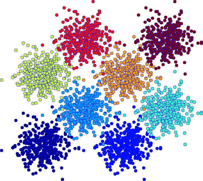
(a)

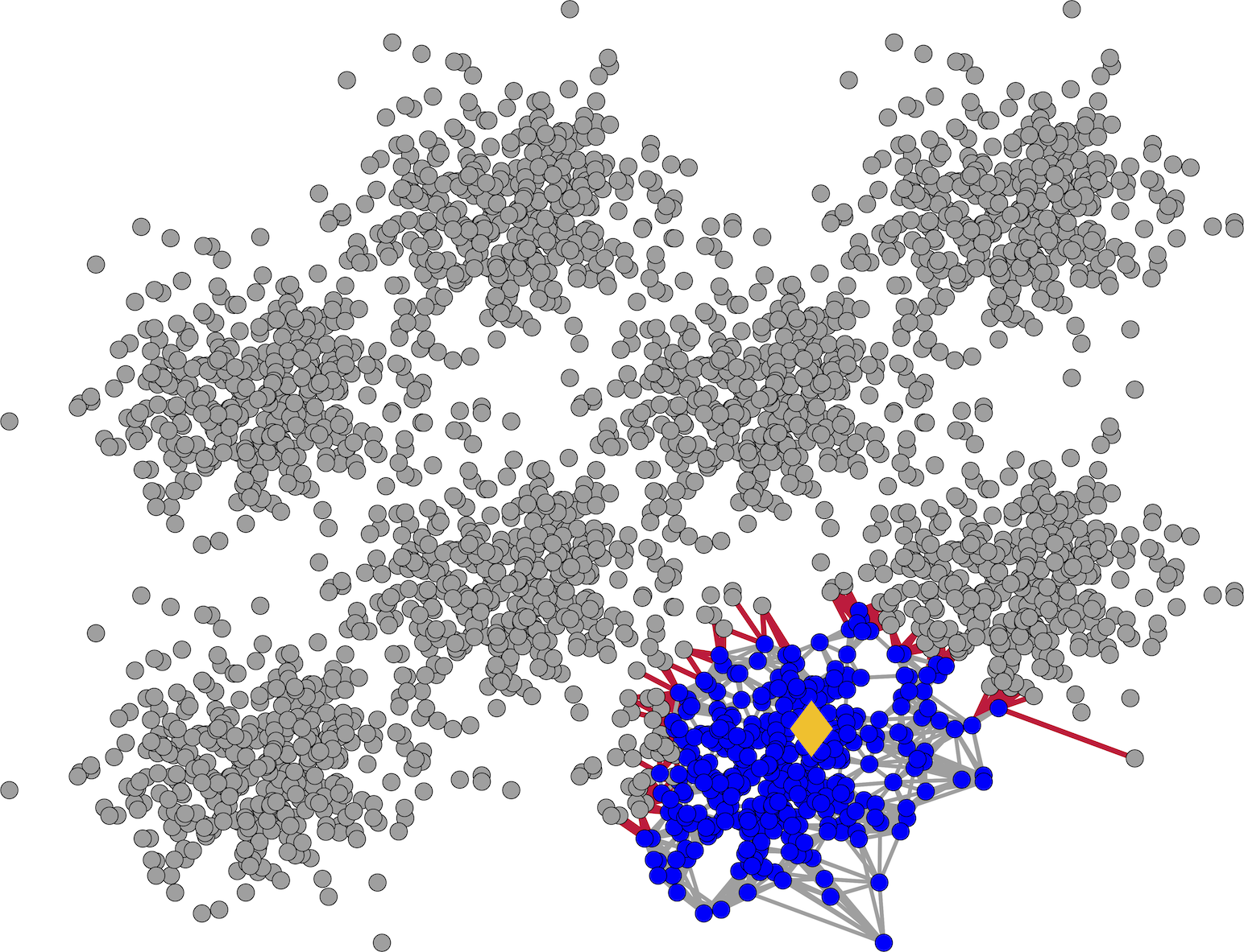
(b)

(c)

(d)

Figure 3: (a) Example of eight groupings. (b) Local cluster based on the NPR problem solution. The starting vertex is shown as a yellow diamond, and the edges comprising the boundary are in red. (c) Conductance and the related (d) $Fscore$ of local clusters for an increasing number of groupings.

6.2.2 Gaussian datasets

Groupings comprised of 400 points in $\mathbb{R}^{2}$ randomly sampled (in each dimension) from a normal distribution with a variance of 0.055 were generated. Their centres were located equidistantly on a square grid. Connectivity between points was established by a nearest neighbour search set to 10 points, i.e., the 10 closest (distance-wise) points to every point were considered connected to that point.

Graphs representing 2, 5, 8, 13, 18, 25, 32, and 41 groupings were constructed. While points are the geometric manifestation or realisation of vertices, edges correspond to the connections between points. The number of edges in each graph was 4,902, 12,153, 19,319, 31,204, 43,013, 59,644, 76,044, and 97,112. Let points be denoted by $y$. For every graph $\mathcal{G}$ and all $\{u,v\}\in\mathcal{E}$, the weight was given by

$$w(u,v)=\exp\left(-4\frac{\lVert y(u)-y(v)\rVert_{2}^{2}}{\nu^{2}}\right),$$

where $\nu$ is the greater distance between $y(u)$ or $y(v)$ and their respective tenth nearest neighbour.

Figure 3(a) depicts an instance of eight groupings as identified by their colour. A local cluster based on the NPR problem solution is highlighted along with the relevant random starting vertex and edge boundary in Figure 3(b). The NPR problem was solved with $\beta=0.0001$ for the 2 and 5 groupings, $\beta=0.001$ for the 8 and 13 groupings, and $\beta=0.005$ for the 18 and more groupings. It can be clearly seen from Figure 3(d) that NPR has the highest mean $Fscore$ for any number of groupings. In comparison, the accuracy of both APPR and $p$-DIFF deteriorates significantly as the number of groupings increases. NPD does not perform badly, but this is at the expense of a greater number of iterations (ten times that suggested in [15]) involved in the solution methodology. With regard to conductance, $p$-DIFF returns the lowest mean values for more than eight groupings, which is visible in Figure 3(c).

(a) $p=1.95$

(b) $p=1.80$

(c) $p=1.60$

Figure 4: Levenberg-Marquardt method for the NPR problem defined on a graph with eight groupings at (a) $p=1.95$, (b) $p=1.8$, and (c) $p=1.6$.

Plots in Figure 4 demonstrate the performance of the Levenberg-Marquardt method for solution of the NPR problem defined on a graph accounting for eight groupings at $p=1.95,1.8$, and $1.6$. As opposed to before, the number of iterations to achieve convergence actually decreases a little as $p$ goes to $1.6$. Note the decrease in mean conductance from $0.014$ to $0.012$, and the increase in mean $Fscore$ from $0.82$ to $0.87$.

6.3 Real-word inspired graphs

6.3.1 Image databases

There is quite the number of image databases that have been developed in order to facilitate research in pattern recognition and machine learning. The MNIST database [7] of handwritten digits from zero to nine has been used extensively. A test set of 10,000 $28\times 28$ grayscale images is provided as part of the database. Similarly, the USPS database [14] contains 11,000 handwritten digit $16\times 16$ grayscale images that were scanned from envelopes in a working post office (by the U.S. Postal Service). Fashion-MNIST [37] is a database that is intended to pose a more significant challenge than the handwritten digits in MNIST. The database offers a test set of 10,000 $28\times 28$ grayscale images from (online retailer) Zalando’s website. Each image is categorised into one of ten classes: t-shirt/top, trouser, pullover, dress, coat, sandals, shirt, sneaker, bag, and ankle boots.

Table 1: Mean conductance and the related mean $Fscore$ of local clusters representing subsets of images in the following databases: MNIST, Fashion-MNIST, and USPS.

		MNIST			Fashion-MNIST			USPS
	$\Phi$		$Fscore$	$\Phi$		$Fscore$	$\Phi$		$Fscore$
NPR	$\mathbf{0.061}\scriptstyle{\pm 1\cdot 10^{-2}}$		$\mathbf{0.710}\scriptstyle{\pm 2\cdot 10^{-1}}$	$\mathbf{0.026}\scriptstyle{\pm 1\cdot 10^{-2}}$		$\mathbf{0.586}\scriptstyle{\pm 2\cdot 10^{-1}}$	$0.094\scriptstyle{\pm 3\cdot 10^{-2}}$		$\mathbf{0.519}\scriptstyle{\pm 1\cdot 10^{-1}}$
APPR	$0.282\scriptstyle{\pm 5\cdot 10^{-2}}$		$0.317\scriptstyle{\pm 1\cdot 10^{-1}}$	$0.234\scriptstyle{\pm 4\cdot 10^{-2}}$		$0.279\scriptstyle{\pm 2\cdot 10^{-1}}$	$\mathbf{0.071}\scriptstyle{\pm 1\cdot 10^{-2}}$		$0.211\scriptstyle{\pm 2\cdot 10^{-2}}$
NPD	$0.135\scriptstyle{\pm 1\cdot 10^{-2}}$		$0.550\scriptstyle{\pm 2\cdot 10^{-1}}$	$0.119\scriptstyle{\pm 4\cdot 10^{-2}}$		$0.451\scriptstyle{\pm 2\cdot 10^{-1}}$	$0.144\scriptstyle{\pm 2\cdot 10^{-2}}$		$0.403\scriptstyle{\pm 2\cdot 10^{-1}}$
$p$-DIFF	$0.111\scriptstyle{\pm 3\cdot 10^{-2}}$		$0.336\scriptstyle{\pm 1\cdot 10^{-1}}$	$0.043\scriptstyle{\pm 1\cdot 10^{-2}}$		$0.317\scriptstyle{\pm 9\cdot 10^{-2}}$	$0.116\scriptstyle{\pm 2\cdot 10^{-2}}$		$0.312\scriptstyle{\pm 2\cdot 10^{-2}}$

Images can be treated as points in Euclidean space of dimension equal to their resolution (i.e., the total number of pixels). Subsequently, graphs were constructed for the aforementioned databases as was done previously. Table 1 presents the mean conductance and related mean $Fscore$ associated with local clusters. Those based on the NPR problem solution have the highest mean $Fscore$ and the lowest conductance in all but one case, which is the USPS database.

Distance (km)

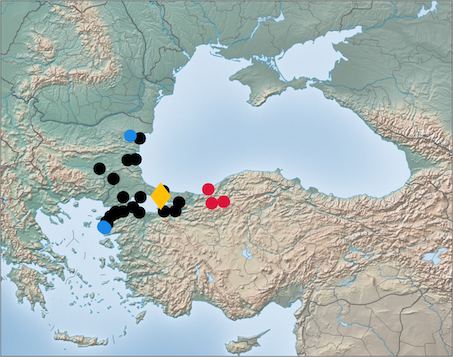
(d) $Fscore=0.875$

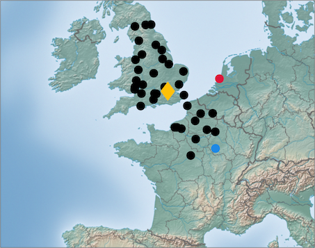
(e) $Fscore=0.974$

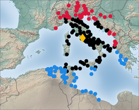
(f) $Fscore=0.709$

Duration (days)

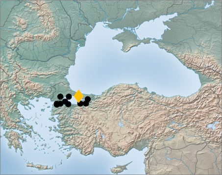
(g) $Fscore=1$

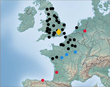
(h) $Fscore=0.929$

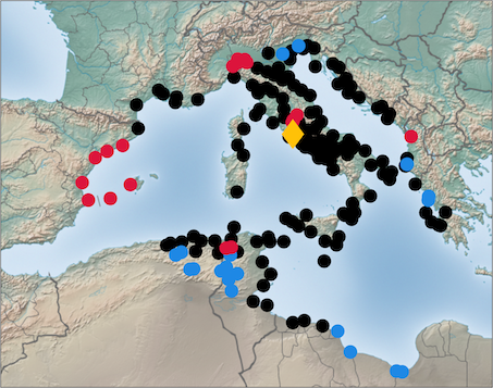
(i) $Fscore=0.885$

Financial cost (denarii)

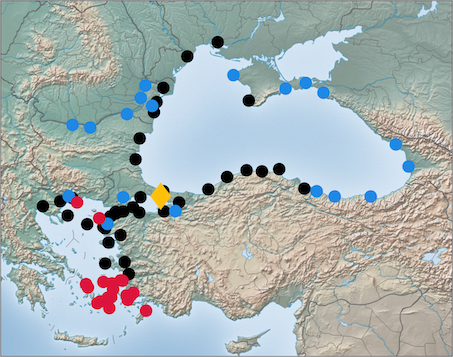
(j) $Fscore=0.672$

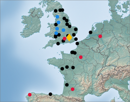
(k) $Fscore=0.848$

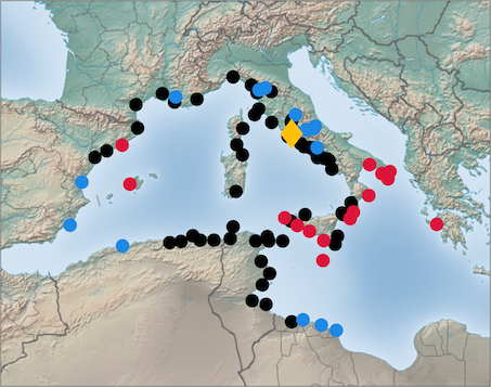
(l) $Fscore=0.803$

Figure 5: Local clusters based on the NPR problem solution in black and blue, and their ground truth equivalent with the same number of vertices in black and red. The number of vertices belonging to a local cluster is (a) 24, (b) 38, (c) 151, (d) 12, (e) 42, (f) 165, (g) 58, (h) 33, and (i) 76. Yellow diamonds represent Constantinopolis (a,d,g), Londinium (b,e,h), and Roma (c,f,i). Clusters are related to the distance (a,b,c), duration (d,e,f), and financial cost (g,h,i) between sites.

6.3.2 Roman world communication network circa 200 AD

ORBIS: The Stanford Geospatial Network Model of the Roman World [34] provides the distance, time and financial cost associated with travel circa 200 AD. The model encompasses a large number of settlements, roads, navigable rivers, and sea lanes that framed movement across the Roman Empire at the time. A disclaimer is in order at this point. There is no intention here whatsoever to make any historically relevant claims. It is only desired to demonstrate the generality of application.

Three graphs were constructed, each with 677 vertices and 1104 edges representing sites and travel routes, respectively. They differed only in weight function definition. For every graph $\mathcal{G}$ and all $\{u,v\}\in\mathcal{E}$, the weight was given by

$$w(u,v)=\exp\left(-2\frac{\chi^{2}}{\iota^{2}}\right),$$

where $\chi$ is the distance, duration, or financial cost between the sites represented by vertices $u$ and $v$. The raw data from ORBIS can have a value for one direction between vertices $u$ and $v$, and another for the opposition direction. An average was, therefore, taken between two values in all cases. $\iota$ is the mean value of the distance, duration, or travel cost between $u$ and adjacent vertices.

A NPR problem solution was obtained for every graph and starting vertex, of which there was three, representing the cities of Constantinopolis (modern day Istanbul, Turkey), Londinium (modern day London, England), and Roma (modern day Rome, Italy). Local clusters were then formed. In order to have a baseline, Dijkstra’s algorithm was utilised to discover the shortest paths (be it distance, time, or financial cost related) from a starting vertex. This provided the rationale for supposed ground truth local clusters. The number of vertices in these clusters was taken to be the same as those in the local clusters based on the NPR problem solution.

Figure 5 visualises the local clusters and their ground truth counterparts. Starting vertices are illustrated by yellow diamonds. Sites coloured black are those that are part of both clusters. While blue sites are those that were not part of the ground truth cluster, the red sites are those that were only part of the ground truth cluster. Other than for two cases, the clusters based on the NPR problem solution were in very good to excellent agreement with the ground truth clusters. Even for those two cases, performance was still respectable with an $Fscore=0.709$ and $Fscore=0.672$. An $Fscore=1$ was registered for the graph with the travel duration edge weight and the starting vertex of Constantinopolis.

References

- [1] S. Amghibech, Eigenvalues of the discrete p-Laplacian for graphs, Ars Combinatoria, 67 (2003), pp. 283–302.
- [2] R. Andersen, F. Chung, and K. Lang, Local graph partitioning using PageRank vectors, in 2006 47th Annual IEEE Symposium on Foundations of Computer Science (FOCS’06), 2006, pp. 475–486, https://doi.org/10.1109/FOCS.2006.44.
- [3] A. Ben-Israel, Generalized inverses of matrices: a perspective of the work of Penrose, Mathematical Proceedings of the Cambridge Philosophical Society, 100 (1986), p. 407–425, https://doi.org/10.1017/S0305004100066172.
- [4] X. Bresson, T. Laurent, D. Uminsky, and J. H. von Brecht, Multiclass total variation clustering, in Proceedings of the 26th International Conference on Neural Information Processing Systems - Volume 1, NIPS’13, 2013, pp. 1421–1429.
- [5] T. Bühler and M. Hein, Spectral clustering based on the graph p-Laplacian, in Proceedings of the 26th Annual International Conference on Machine Learning, ICML ’09, 2009, pp. 81–88, https://doi.org/10.1145/1553374.1553385.
- [6] S. L. Campbell and C. D. Meyer, Generalized Inverses of Linear Transformations, Society for Industrial and Applied Mathematics, 2009, https://doi.org/10.1137/1.9780898719048.
- [7] L. Deng, The MNIST database of handwritten digit images for machine learning research [best of THE WEB], IEEE Signal Processing Magazine, 29 (2012), pp. 141–142, https://doi.org/10.1109/MSP.2012.2211477.
- [8] E. W. DIJKSTRA, A note on two problems in connexion with graphs., Numerische Mathematik, 1 (1959), pp. 269–271, https://doi.org/10.1007/BF01386390.
- [9] A. Dresden, The fourteenth western meeting of the American Mathematical Society, Bulletin of the American Mathematical Society, 26 (1920), pp. 385–396, https://doi.org/10.1090/S0002-9904-1920-03322-7.
- [10] D. Floros, T. Liu, N. Pitsianis, and X. Sun, Fast graph algorithms for superpixel segmentation, in 2022 IEEE High Performance Extreme Computing Conference (HPEC), 2022, pp. 1–8, https://doi.org/10.1109/HPEC55821.2022.9926359.
- [11] K. Fountoulakis, D. Wang, and S. Yang, p-norm flow diffusion for local graph clustering, in Proceedings of the 37th International Conference on Machine Learning, ICML’20, 2020, pp. 3222–3232.
- [12] D. Gleich and M. Polito, Approximating personalized PageRank with minimal use of web graph data, Internet Mathematics, 3 (2006), pp. 257 – 294, https://doi.org/10.1080/15427951.2006.10129128.
- [13] R. A. Horn and C. R. Johnson, Matrix Analysis, Cambridge University Press, 2 ed., 2012.
- [14] J. J. Hull, A database for handwritten text recognition research, IEEE Transactions on Pattern Analysis and Machine Intelligence, 16 (1994), pp. 550–554, https://doi.org/10.1109/34.291440.
- [15] R. Ibrahim and D. Gleich, Nonlinear diffusion for community detection and semi-supervised learning, in The World Wide Web Conference, 2019, pp. 739–750, https://doi.org/10.1145/3308558.3313483.
- [16] Y. Ijiri, On the generalized inverse of an incidence matrix, Journal of the Society for Industrial and Applied Mathematics, 13 (1965), pp. 827–836, https://doi.org/10.1137/0113053.
- [17] I. C. F. Ipsen, C. T. Kelley, and S. R. Pope, Rank-deficient nonlinear least squares problems and subset selection, SIAM Journal on Numerical Analysis, 49 (2011), pp. 1244–1266, https://doi.org/10.1137/090780882.
- [18] C. T. Kelley, Iterative Methods for Optimization, Society for Industrial and Applied Mathematics, 1999, https://doi.org/10.1137/1.9781611970920.
- [19] G. Kollias, E. Gallopoulos, and A. Grama, Surfing the network for ranking by multidamping, IEEE Transactions on Knowledge and Data Engineering, 26 (2014), pp. 2323–2336, https://doi.org/10.1109/TKDE.2013.15.
- [20] A. Lancichinetti, S. Fortunato, and F. Radicchi, Benchmark graphs for testing community detection algorithms, Phys. Rev. E, 78 (2008), p. 046110, https://doi.org/10.1103/PhysRevE.78.046110.
- [21] M. Liu and D. F. Gleich, Strongly local p-norm-cut algorithms for semi-supervised learning and local graph clustering, in Proceedings of the 34th International Conference on Neural Information Processing Systems, NIPS ’20, 2020, pp. 5023–5035.
- [22] D. Luo, H. Huang, C. Ding, and F. Nie, On the eigenvectors of p-Laplacian, Machine Learning, 81 (2010), pp. 37–51, https://doi.org/10.1007/s10994-010-5201-z.
- [23] E. H. Moore, General Analysis, Part I, The American Philosophical Society, Philadelphia, 1935.
- [24] A. Y. Ng, M. I. Jordan, and Y. Weiss, On spectral clustering: Analysis and an algorithm, in Proceedings of the 14th International Conference on Neural Information Processing Systems: Natural and Synthetic, NIPS’01, 2001, pp. 849–856.
- [25] H. Nielsen and C. Völcker, IMMOPTIBOX: A matlab toolbox for optimization and data fitting, 2010.
- [26] J. Nocedal and S. J. Wright, Numerical Optimization, Springer, 1999.
- [27] D. Pasadakis, C. L. Alappat, O. Schenk, and G. Wellein, Multiway p-spectral graph cuts on Grassmann manifolds, Machine Learning, 111 (2022), pp. 791–829, https://doi.org/10.1007/s10994-021-06108-1.
- [28] D. Pasadakis, M. Bollhöfer, and O. Schenk, Sparse quadratic approximation for graph learning, IEEE Transactions on Pattern Analysis and Machine Intelligence, 45 (2023), pp. 11256–11269, https://doi.org/10.1109/TPAMI.2023.3263969.
- [29] M. H. Pearl, On generalized inverses of matrices, Mathematical Proceedings of the Cambridge Philosophical Society, 62 (1966), pp. 673–677, https://doi.org/10.1017/S0305004100040329.
- [30] R. Penrose, A generalized inverse for matrices, Mathematical Proceedings of the Cambridge Philosophical Society, 51 (1955), p. 406–413, https://doi.org/10.1017/S0305004100030401.
- [31] R. J. Plemmons, -matrix characterizations.I—nonsingular -matrices, Linear Algebra and its Applications, 18 (1977), pp. 175–188, https://doi.org/10.1016/0024-3795(77)90073-8.
- [32] A. Quarteroni, R. Sacco, and F. Saleri, Numerical Mathematics, Springer Berlin Heidelberg, 2006, https://doi.org/10.1007/b98885.
- [33] S. Saito and M. Herbster, Multi-class graph clustering via approximated effective p-resistance, in Proceedings of the 40th International Conference on Machine Learning, ICML’23, 2023, pp. 29697–29733.
- [34] W. Scheidel, ORBIS: The Stanford geospatial network model of the Roman world, Princeton/Stanford Working Papers in Classics, (2015), https://doi.org/10.2139/ssrn.2609654.
- [35] F. Tudisco and M. Hein, A nodal domain theorem and a higher-order Cheeger inequality for the graph p-Laplacian, Journal of Spectral Theory, 8 (2018), pp. 883–908, https://doi.org/10.4171/JST/216.
- [36] U. von Luxburg, A tutorial on spectral clustering, Statistics and computing, 17 (2007), pp. 395–416, https://doi.org/10.1007/s11222-007-9033-z.
- [37] H. Xiao, K. Rasul, and R. Vollgraf, Fashion-MNIST: A novel image dataset for benchmarking machine learning algorithms, Sept. 2017, https://arxiv.org/abs/1708.07747.