When Does Visual Prompting Outperform Linear Probing for Vision-Language Models? A Likelihood Perspective

Abstract

Adapting pre-trained models to new tasks can exhibit varying effectiveness across datasets. Visual prompting, a state-of-the-art parameter-efficient transfer learning method, can significantly improve the performance of out-of-distribution tasks. On the other hand, linear probing, a standard transfer learning method, can sometimes become the best approach. We propose a log-likelihood ratio (LLR) approach to analyze the comparative benefits of visual prompting and linear probing. By employing the LLR score alongside resource-efficient visual prompts approximations, our cost-effective measure attains up to a 100-fold reduction in run time compared to full training, while achieving prediction accuracies up to 91%. The source code is available at VP-LLR.

1 Introduction

When applying transfer learning to downstream tasks, specific modifications to the pre-trained model are required. For instance, linear probing (LP) involves adjusting the linear layer in the model’s penultimate layer, while full fine-tuning involves modifying all parameters in the model. However, in the emerging field of fine-tuning for transfer learning, visual prompting (VP) Chen (2024); Bahng et al. (2022) offers a method that does not necessitate changes to the pre-trained model.

Specifically, studies such as CLIP-VP Bahng et al. (2022) and AutoVP Tsao et al. (2024) indicate that visual prompting is particularly suitable for out-of-distribution (OOD) datasets. In AutoVP, the authors observed that datasets with lower confidence scores, indicative of being more OOD, tend to achieve greater accuracy gains (i.e., the performance difference between VP and LP).

In this paper, we conduct an in-depth analysis of the effects of visual prompts on both OOD and in-distribution (ID) datasets. In Fig. 1, we compute the Pearson correlation coefficient (PCC) Cohen et al. (2009); Zhang et al. (2020) of model embeddings. The PCC is computed from embeddings generated by inputting the entire prompted image versus the image or prompt separately. The result (prompts or images) with a higher PCC score indicates greater similarity to the embedding obtained from the full input (i.e., the prompted image), indicating that it provides the dominant feature. The results show that in OOD datasets, prompts achieve a PCC of 0.9 in shallow layers, while in ID datasets, the output logits of clean images reach a PCC of 0.91. This implies that OOD datasets are better suited for training with VP, while ID datasets, to avoid interference with the inherent features of the image, are more appropriate for training with LP.

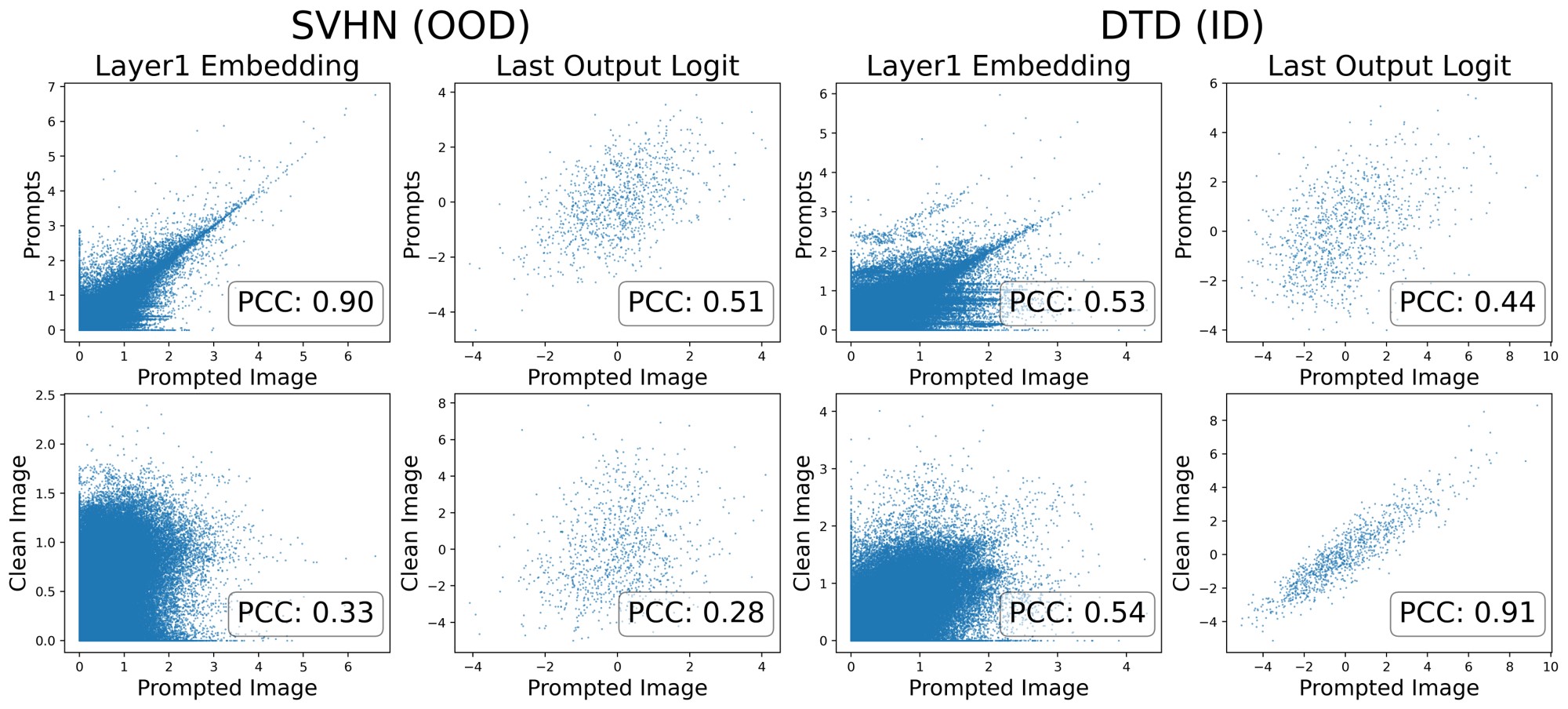
Figure 1: The PCC of Embeddings in ResNet18. The $PCC_{X,Y}$ is calculated by embeddings $X$ and $Y$. Here, $X$ is obtained by inputting the entire prompted image, while $Y$ is obtained by inputting either (1) the visual prompts or (2) the clean image.

Since there is no one-fits-all method, selecting an applicable transfer learning method for downstream datasets remains critical. Some training-free approaches can serve as reliable references for estimating models’ adaptability to downstream datasets, thereby preventing the need to explore the large space of the training configurations. Several studies have focused on pre-trained model selection Nguyen et al. (2020); Tran et al. (2019); You et al. (2021). Building on this idea, we extend LogME You et al. (2021) to the selection of methods, VP or LP, providing a log-likelihood ratio (LLR) method as described in Section 3.1. Table 1 presents the execution time across various methods, with an overall speedup of 100 times compared to linear probing (LP).

We summarize the main contributions as follows:

• We propose a cost-effective log-likelihood ratio (LLR) method to estimate whether VP or LP offers greater advantages on a given dataset.

• The LLR scores effectively reflect the proportions of ID/OOD data in the dataset and align well with the accuracy differences between VP and LP.

• The comprehensive results on 12 datasets (Section 4.2) using LLR scores outperform OOD detection baselines.

2 Background and Related Work

2.1 Visual Prompting

Visual prompting (VP), also known as model reprogramming Elsayed et al. (2019), can be used to adapt a pre-trained model to new tasks. The VP framework, as shown in Fig. 2, consists of three components: input transformation, pre-trained models, and output transformation. In the input transformation, a trainable visual prompt is added, typically in the form of a frame padded around the image. The pre-trained model serves as a feature extractor and remains frozen during VP training. The output transformation then maps the pre-trained model’s source labels to the target labels of the downstream task. Previous studies have investigated various VP designs and usage scenarios, including exploration of optimal prompt sizes Bahng et al. (2022); Tsao et al. (2024), visual prompt tuning in vision transformers Jia et al. (2022), black-box VP training Tsai et al. (2020), and iterative approaches to learning output mappings Chen et al. (2023). These studies have demonstrated the capability and computational efficiency of VP.

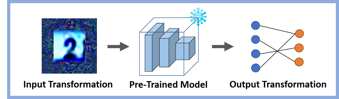
Figure 2: The Visual Prompting Framework.

2.2 LogME for Model Selection

Before performing model finetuning, maximum likelihood estimation methods can be used to select the most suitable pre-trained model for training. LogME You et al. (2021) employs evidence (i.e. marginalized likelihood) to assess the predictive capability of a model. The evidence is described as follows:

$$p(y|F,\alpha,\beta)=\int_{w}p(w|\alpha)p(y|F,w,\beta)dw$$ (1)

where $y$ is the target label, $w$ follows an isotropic multivariate Gaussian distribution, representing the parameter of the linear layer added on top of the pre-trained model. $F=\{f_{i}\in\mathbb{R}^{D}\}_{i=1}^{n}$ is the feature matrix of dimension $D$ obtained from the model’s last layer, and $\alpha^{-1}$ and $\beta^{-1}$ are the variances of $w$ and the prediction $y$, respectively. The log-likelihood can be further derived as follows You et al. (2021); Bishop and Nasrabadi (2006), where $A=\alpha I+\beta F^{T}F$ and $m=\beta A^{-1}F^{T}y$:

$$\begin{split}\log(p(y|F,\alpha,\beta))&=\frac{D}{2}log(\alpha)+\frac{n}{2}log(\beta)-\frac{n}{2}log(2\pi)\\ &-\frac{\alpha}{2}m^{T}m-\frac{\beta}{2}{||Fm-y||}^{2}-\frac{1}{2}log(|A|)\\ \end{split}$$ (2)

Following, the maximized value in Equation 2 with optimized variances $\alpha^{*}$ and $\beta^{*}$ is the LogME score.

3 Methodology

3.1 Log-Likelihood Ratio

To evaluate the comparative performance of the linear probing (LP) model $\theta$ and the visual prompting (VP) model $\theta_{p}$ with the given dataset, we utilize the log-likelihood ratio (LLR) method described in Equation 3. The terms $p_{\theta}$ and $p_{\theta_{p}}$ denote the maximum likelihoods of LP and VP, respectively. By decomposing the input $x$ into components $x_{ID}$ and $x_{OOD}$, we can analyze the distinct impacts of visual prompts on ID and OOD inputs. As discussed in Section 1, in ID datasets, prompts may disrupt the dominant features from the clean images, resulting in an LLR score below 0 (LLR: Dominant ID Features). Conversely, for OOD datasets, prompts enhance the model’s recognition ability by providing crucial features, yielding an LLR score above 0 (LLR: Dominant OOD Features).

$$\begin{split}&LLR(x):=\log\frac{p_{\theta_{p}}(x)}{p_{\theta}(x)}=\log\text{ }p_{\theta_{p}}(x)-log\text{ }p_{\theta}(x)\\ &:=\log(p_{\theta_{p}}(x_{ID})p_{\theta_{p}}(x_{OOD}))-\log(p_{\theta}(x_{ID})p_{\theta}(x_{OOD}))\end{split}$$ (3)

$$\begin{split}&LLR(x)\sim\log\text{ }p_{\theta_{p}}(x_{ID})-\log\text{ }p_{\theta}(x_{ID})<0\end{split}$$ (LLR: Dominant ID Features)

$$\begin{split}&LLR(x)\sim\log\text{ }p_{\theta_{p}}(x_{OOD})-\log\text{ }p_{\theta}(x_{OOD})>0\end{split}$$ (LLR: Dominant OOD Features)

3.2 LogME Evidence and Visual Prompting Evidence

To obtain the maximum log-likelihood $\log p_{\theta}$, we follow the method in LogME You et al. (2021), as described in Section 2.2. When considering the VP model, the impact of visual prompts is reflected in the feature matrix as $F(\delta)$. Therefore, $\log p_{\theta_{p}}$ can be obtained from equation LogME-VP , which involves computing the expectation value of the evidence with respect to the visual prompt $\delta$.

$$\begin{split}p(y|F,\alpha,\beta)&=\int_{w}p(w|\alpha){\color[rgb]{0,0,0}\int_{\delta}p(\delta)}p(y|{\color[rgb]{0,0,0}F(\delta)},w,\beta,{\color[rgb]{0,0,0}\delta}){\color[rgb]{0,0,0}d\delta}dw\\ &={\color[rgb]{0,0,0}\int_{\delta}p(\delta)}\underbrace{\int_{w}p(w|\alpha)p(y|{\color[rgb]{0,0,0}F(\delta)},w,\beta,{\color[rgb]{0,0,0}\delta})dw}_{\text{Evidence}}{\color[rgb]{0,0,0}d\delta}\\ &=\mathbb{E}_{\delta}[\text{Evidence}({\color[rgb]{0,0,0}\delta})];\\ \log(p(y|F,\alpha,\beta))&=\mathbb{E}_{\delta}[\log\big{(}\text{Evidence}({\color[rgb]{0,0,0}\delta})\big{)}]\end{split}$$ (LogME-VP)

At this stage, once $\log p_{\theta{p}}$ and $\log p_{\theta}$ are calculated, subtracting the two provides the LLR scores in Equation 3.

3.3 Visual Prompt Approximation

Table 1: Comparison of Linear Probing (LP), Full Fine-Tuning (FF), and the LLR Score with Simulated Visual Prompts. Using the EuroSAT dataset and CLIP as the pre-trained model, the table presents execution time, trainable parameter size, and training dataset size for each method.

Experimental Info.	LP	FF	LLR (a) Gaussian	LLR (b) Gradient	LLR (c) Mini-FT	LLR (d) Mini-FT-5R
Execution Time (second)	2370	3081	22	27	23	33
Trainable Parameter Size (Million)	0.005	151.28	0	0	0.15	0.15
Training Dataset Size	13,500	13,500	0	$\sim$1,000	$\sim$1,000	$\sim$1,000

Given the vastness of the $\mathbb{R}^{3\times N\times N}$ prompt space for images, exhaustively exploring all visual prompts to compute the expectation value in LogME-VP is impractical. Hence, we explore different methods for simulating prompt distributions. These methods can be categorized into two approaches: the training-free approach and the mini-finetuning approach.

(i) Training-Free Approach: We employ two distributions to model visual prompts. The first one is an isotropic multivariate Gaussian distribution, which simulates prompts $\delta\sim N(0,\gamma I)$ with standard deviation $\gamma$. The second method is the gradient approximation approach, where prompts’ gradients are computed from a small subset ($\sim$1k) of samples $\{x_{i}\}^{n}_{i=1}$ Krishnamachari et al. (2023) and the loss function $E$ is minimized via Taylor expansion approximation Tang et al. (2024); Hsiung et al. (2023) (see Equation 4).

$$\begin{split}&E(x+\delta)\approx E(x)+\delta^{T}\bigtriangledown E(x)\\ &{\nabla E(x)}_{i}=g_{i}\text{, the gradient respected to pixel $i$}.\\ &\text{minimize: }\delta^{T}\nabla E(x)=\delta^{T}\textbf{g}=\sum\delta_{i}g_{i}\\ &\Rightarrow\left\{\begin{aligned} &g_{i}\geq 0\rightarrow\delta_{i}=0\\ &g_{i}<0\rightarrow\delta_{i}=1\text{, for pixel value $\delta_{i}$}\in[0,1].\end{aligned}\right.\end{split}$$ (4)

(ii) Mini-Finetuning: We select a small subset of samples and exclusively update the prompts. This process is conducted under two configurations: 1&5-epoch tuning.

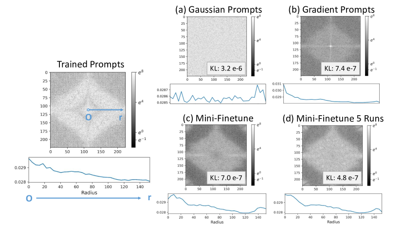
Figure 3: The Similarity of Visual Prompts on CLIP (ViT/B-32). Various types of prompts are presented in the frequency domain, along with line plots of the average values with radii. The similarity between simulated and trained visual prompts is evaluated using KL divergence Kullback and Leibler (1951).

Fig. 3 (a) to (d) shows the distribution of the four simulated prompts in the frequency domain. From method (a) to (b) and referring to Table 1, there is an increase in data utilization, moving from a data-free approach to a limited-data setting. Subsequently, from (c) to (d), the computation increases fivefold for the tuning process. This demonstrates that with increased resources, whether data or computation, the simulated prompts can approximate the trained ones more closely, validated by the decrease in KL divergence between their distributions.

4 Experimental Results

Table 2: LLR Sorting Results. The evaluated metrics include Kendall’s $\tau$ in green, Spearman’s $\rho$ in red, and LLR-Acc (%) in blue. The highest score is underlined (excluding scores from trained prompts). The baseline methods (see Appendix E) include the confidence score Hendrycks and Gimpel (2017), the ODIN confidence score Liang et al. (2018), and AUROC with Mahalanobis Distance Lee et al. (2018).

	Trained Prompts	Without Prompts	Gaussian	Gradient	Mini-Finetune	Mini-Finetune 5 Rounds	Confidence Score	ODIN Confidence	Mahalanobis Distance AUROC
ResNet18	0.61 0.77 75.0	0.67 0.83 41.7	0.48 0.65 58.3	0.52 0.71 58.3	0.42 0.62 58.3	0.45 0.61 58.3	0.27 0.41	0.21 0.31	0.52 0.69
ResNext-IG	0.58 0.78 83.3	0.18 0.24 50.0	0.61 0.73 66.7	0.64 0.80 83.3	0.33 0.48 58.3	0.27 0.38 58.3	0.52 0.70	0.33 0.47	0.38 0.60
ViT-B-16	0.61 0.81 66.7	0.42 0.66 75.0	0.58 0.77 91.7	0.64 0.82 91.7	0.48 0.63 91.7	0.48 0.64 91.7	0.18 0.18	-0.18 -0.31	0.61 0.77
Swin-T	0.58 0.80 91.7	0.39 0.56 50.0	0.42 0.67 83.3	0.42 0.63 83.3	0.48 0.69 83.3	0.70 0.81 91.7	0.48 0.73	0.39 0.59	0.52 0.73
CLIP(VIT/B-32)	0.64 0.84 83.3	0.27 0.38 50.0	0.55 0.73 66.7	0.55 0.69 66.7	0.61 0.79 66.7	0.52 0.71 75.0	0.39 0.62	0.15 0.15	0.45 0.61

In this section, we will demonstrate the efficacy of the proposed LLR scores and simulated prompts. These techniques will be utilized to rank datasets according to the accuracy gains achieved by VP compared to LP.

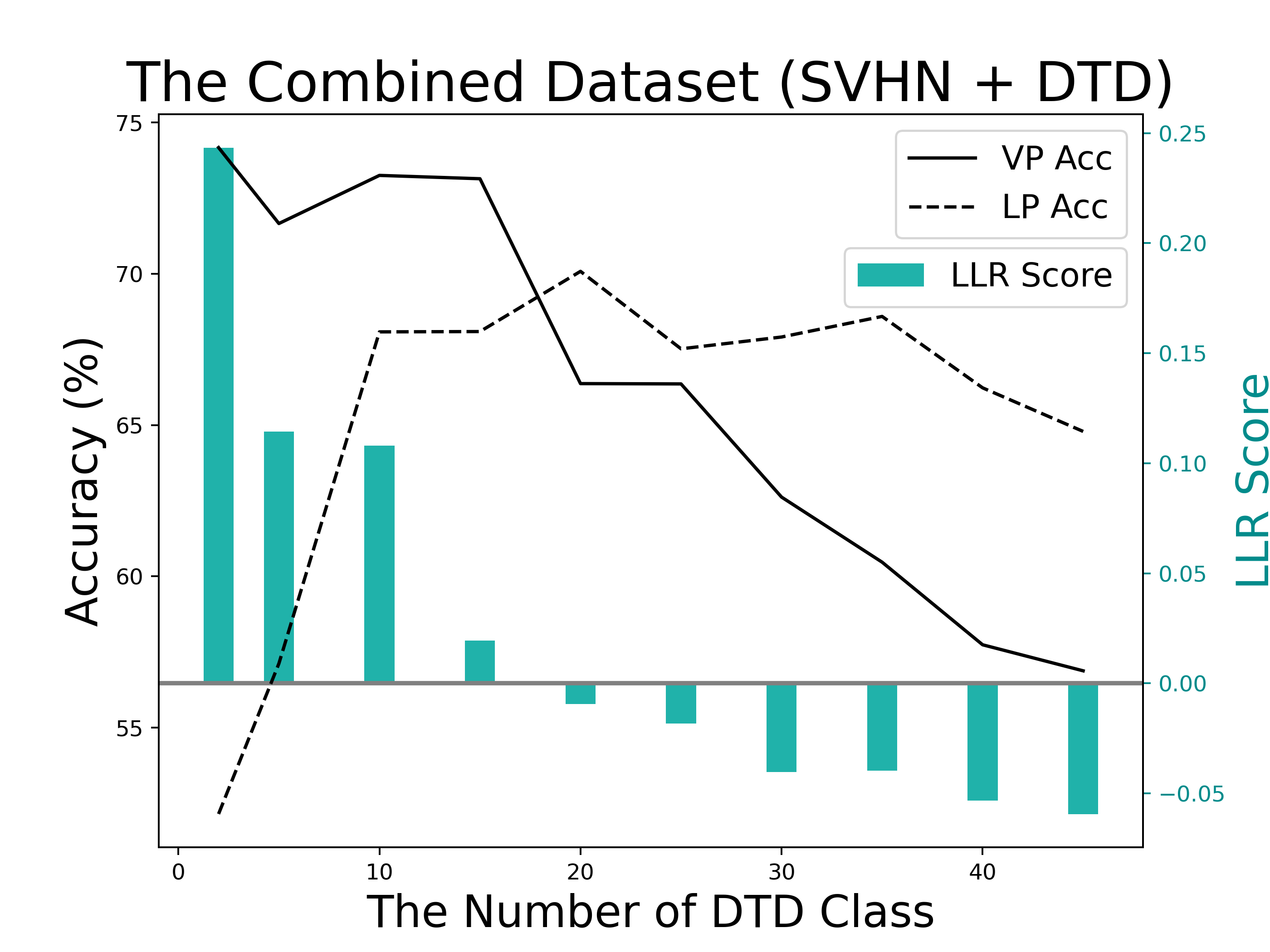
Figure 4: Accuracy and LLR on the Combined Datasets Using CLIP (ViT-B/32). SVHN is considered more OOD, while DTD tends to be ID. There are 10 classes in SVHN, and we gradually increase the number of classes in DTD from 2 to 45 to obtain different ID/OOD proportions.

4.1 The Effectiveness of LLR and Simulated Prompts

LLR scores in Section 3.1 are utilized to differentiate the impact of visual prompts on ID/OOD datasets. In Fig. 4, using a mixed dataset as an example, we observe a close correlation between LLR scores and actual accuracy gains, indicating the method effectively identifies whether VP or LP provides an advantage. A positive LLR score suggests that datasets (leaning towards OOD) benefit more from VP training, while a negative LLR score indicates that datasets (leaning towards ID) are more suitable for LP training.

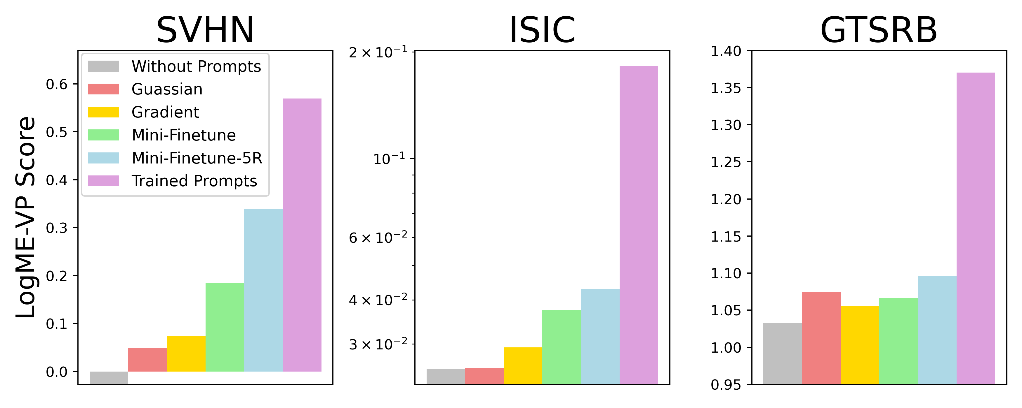
Figure 5: The LogME-VP Scores with Prompts. The plot shows the LogME-VP scores obtained from CLIP (ViT-B/32) with various input prompts, including without prompts, Gaussian prompts, gradient prompts, mini-finetuning prompts, and well-trained prompts.

Furthermore, we have validated the efficacy of the simulation methods proposed in Section 3.3. From two aspects – the distributional fidelity indicated by decreasing KL divergence (Fig. 3) and increasing LogME-VP scores (Fig. 5)—show that the simulated prompts progressively converge towards those obtained from the trained prompts.

4.2 The Sorting Results with Diverse Datasets

We applied the proposed LLR method to 12 downstream datasets and 5 pre-trained models (see Appendix A). To evaluate the performance of the LLR scores, we used ranking coefficients such as Kendall’s $\tau$ Kendall (1938) and Spearman’s $\rho$ Spearman (1904) to assess the alignment between LLR scores and accuracy gains. Additionally, $\text{LLR-Acc}=\frac{\textbf{TP}+\textbf{FN}}{n}$ measures the proportion of datasets that remain in the correct quadrant, with TP representing true positives (positive gains with positive LLR scores) and FN representing false negatives (negative gains with negative LLR scores). The performance gains are obtained from Bahng et al. (2022) for LP and from AutoVP Tsao et al. (2024) for VP.

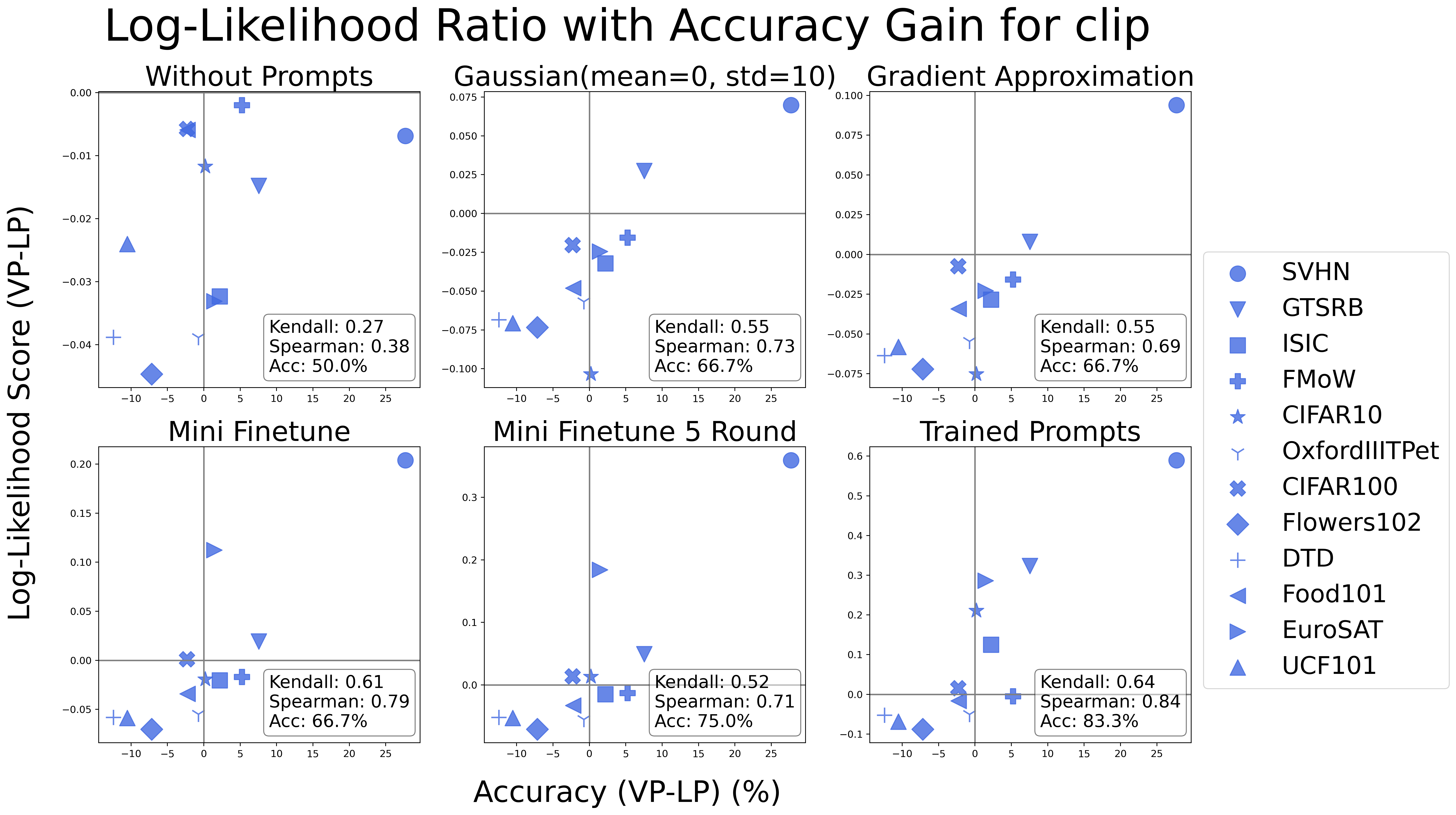
Figure 6: The Sorting Results with Simulated Prompts. The accuracy gains obtained from CLIP (ViT-B/32) are sorted by the LLR scores.

The visualization of the sorting results with CLIP is presented in Fig. 6. It is clear that the inclusion of simulated prompts significantly enhances both the ranking scores and LLR-Acc compared to the scenario without prompts. Additionally, the overall performance are detailed in Table 2. Our LLR method outperforms all baseline methods for OOD detection, offering a more accurate estimation of accuracy gains. This enhanced performance is attributed to precise likelihood calculations and the incorporation of prompt approximations that closely align with the design of visual prompting. Based on these results, utilizing LLR scores facilitates a more accurate determination of the appropriate training approach. Specifically, datasets with higher LLR scores are more suitable for visual prompting, while lower LLR scores indicate a better fit for linear probing.

5 Conclusion

This paper proposes an LLR score using visual prompt approximation methods to evaluate the advantage of VP over LP. The LLR scores demonstrate improved ranking with actual accuracy gains and reliable performance prediction, effectively correlating with the proportion of OOD data in the dataset. Consequently, this approach serves as a valuable precursor for training in transfer learning, significantly reducing the time for exploring different fine-tuning methods.

Appendix

Appendix A Datasets and Pre-Trained Models

We employed 12 datasets for LLR sorting in Section 4.2. Detailed information is provided in Table 3. We utilized five pre-trained models: the convolutional-based models (ResNet18 He et al. (2016) and ResNext-IG Mahajan et al. (2018)), vision transformers (ViT-B-16 Dosovitskiy et al. (2020) and Swin-T Liu et al. (2021)), and the multi-modal model (CLIP Radford et al. (2021)). ResNext-IG is pre-trained on billions of Instagram images with 1000 classes. CLIP is trained using image-text pairs as input, enabling zero-shot prediction without a fixed predicted class number. The remaining models are pre-trained on ImageNet-1K Russakovsky et al. (2015), which includes 1000 distinct labels.

Table 3: Dataset Information. The table shows the number of classes for each dataset and the respective LP Bahng et al. (2022) and VP Tsao et al. (2024) accuracy (%) with CLIP.

Dataset	Class Number	LP Accuracy	VP Accuracy
SVHN Netzer et al. (2011)	10	65.4	93.1
EuroSAT Helber et al. (2019)	10	95.3	96.8
Flowers102 Nilsback and Zisserman (2008)	102	96.9	89.7
CIFAR100 Krizhevsky and Hinton (2009)	100	80.0	77.7
UCF101 Soomro et al. (2012)	101	83.3	72.8
DTD Cimpoi et al. (2014)	47	74.6	62.2
FMoW Christie et al. (2018)	62	36.3	41.5
GTSRB Houben et al. (2013)	43	85.8	93.4
CIFAR10 Krizhevsky and Hinton (2009)	10	95.0	95.2
Food101 Bossard et al. (2014)	101	84.6	82.4
OxfordIIITPet Parkhi et al. (2012)	37	89.2	88.4
ISIC Codella et al. (2019); Tschandl et al. (2018)	7	71.9	74.1

Appendix B VP and LP Performance

The performance gains are obtained from the accuracy difference between VP and LP. Therefore, we use the LP accuracy from Bahng et al. (2022), and VP accuracy from AutoVP Tsao et al. (2024). For pre-trained models not included in these works, we trained them ourselves using the same settings. In VP, the output mapping is FullyMap (as described in AutoVP Section 3), with prompt frame sizes of 48 for SVHN and 16 for the other datasets.

Appendix C Feature Extraction for Evidence Score Calculation

When calculating the LogME scores, the feature $F$ is derived from the output of the pre-trained model, which serves as a feature extractor. Due to the differences in the frameworks of VP and LP, the features extracted for computing the evidence scores vary. Details can be found in Fig. 7. For LP, the pre-trained model’s linear classifier is adjusted for adaptation, so the feature $F$ is extracted from the output of the pre-trained model. However, since the VP model retains the pre-trained output classifier and obtains a mapping (e.g., FullyMap), the $F(\delta)$ is extracted from the model’s linear classifier (i.e. FC in Fig. 7). Additionally, the dimensions of $F$ vary depending on the extraction point. Table 4 show the dimensions of $F$ under different frameworks.

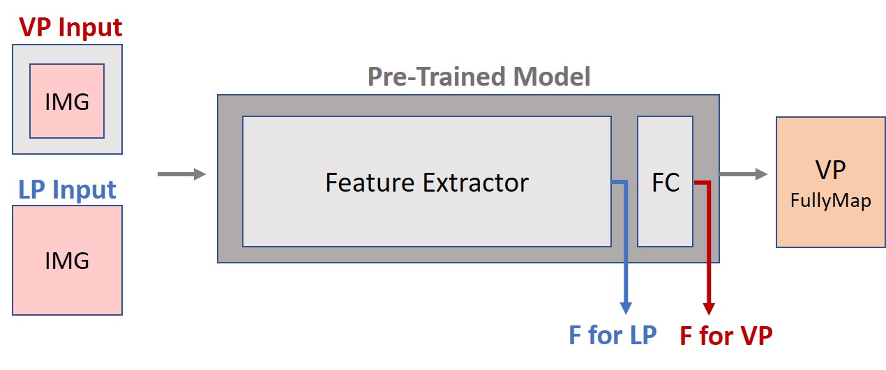
Figure 7: Feature Extraction for VP and LP. The symbols marked in blue and red represent the features used for computing the evidence score for LP and VP, respectively, and are extracted from different layers of the pre-trained model.

Table 4: Feature Dimension of VP and LP. $N$ represents the input sample size. In CLIP, 81 is the number of text templates used, and $Cls\_Num$ denotes the number of classes in the dataset.

Framework	ResNet18	IG	ViT-B	Swin-T	CLIP-VIT/B-32
VP Feature Dimension	(N,1000)	(N,1000)	(N,1000)	(N,1000)	(N,81*$Cls\_Num$)
LP Feature Dimension	(N,512)	(N,2048)	(N,768)	(N,768)	(N,512)

Appendix D Sorting Metrics

In Section4.2, we introduce three metrics to evaluate the performance of the LLR sorting results. The ranking metrics, Kendall’s $\tau$ coefficient and Spearman’s $\rho$ coefficient, range from -1 to 1, where 1 indicates a perfectly correct ranking, and -1 indicates a completely reversed ranking. Kendall’s $\tau$ serves as a more rigorous metric, necessitating verification of the correct ordering for each pair of items, whereas Spearman’s correlation is comparatively less stringent, derived from the summation of the squared differences of the ranks.

$$\tau(\textbf{X},\textbf{Y})=\frac{2}{n(n-1)}\sum_{i<j}sgn(x_{i}-x_{j})sgn(y_{i}-y_{j}) \tau$$ (Kendall’s coefficient)

$$\rho(\textbf{X},\textbf{Y})=1-\frac{6\sum_{i}d_{i}^{2}}{n(n^{2}-1)}\text{, where }d_{i}=Rank(x_{i})-Rank(y_{i}) \rho$$ (Spearman’s coefficient)

The final metric, as shown in Equation LLR-Accuracy, calculates the ratio of true positives (TP) and false negatives (FN) to the total data point $n$. When the LLR score is accurately estimated, positive LLR correspond to positive accuracy gains (TP points), while negative LLR correspond to negative accuracy gains (FN points).

$$Acc(\textbf{X},\textbf{Y})=\frac{\textbf{TP}+\textbf{FN}}{n}$$ (LLR-Accuracy)

Appendix E OOD Detection Baselines

In Section 1, we assert that data tending to be OOD may exhibit larger accuracy gains, while data tending to be ID may show smaller or even negative accuracy gains. Therefore, in Section 4.2, we utilize several OOD detection techniques as baseline methods for comparison with our LLR scores. The OOD detection baselines as detailed below:

• Confidence score Hendrycks and Gimpel (2017), defined as the maximum class probability from a softmax classifier, is represented as $p(\hat{y}|x)=max_{c}\text{ }p(y=c|x)$, where label $c$ is from $1\sim N$ and $x$ is the input samples. Higher scores indicate ID data, while lower scores indicate OOD data.

• ODIN confidence Liang et al. (2018) employs techniques such as temperature scaling and adding small perturbations to the input better to separate confidence scores of ID and OOD samples.

• Mahalanobis distance Lee et al. (2018), $M_{\ell}=min_{c}(f_{\ell}(x)-\mu_{\ell,c})^{T}\Sigma_{\ell}^{-1}(f_{\ell}(x)-\mu_{\ell,c})$, computes the closest Gaussian distance from the training classes $c$ by using the features of layer $\ell$ in pre-trained models. We use the output AUROC scores for sorting; higher AUROC indicates more OOD.

For methods using confidence scores and ODIN confidence, we add a negative sign before sorting, as higher scores indicate ID data, which is the opposite trend to our LLR perspective.

Appendix F LogME For Visual Prompting Model Ranking

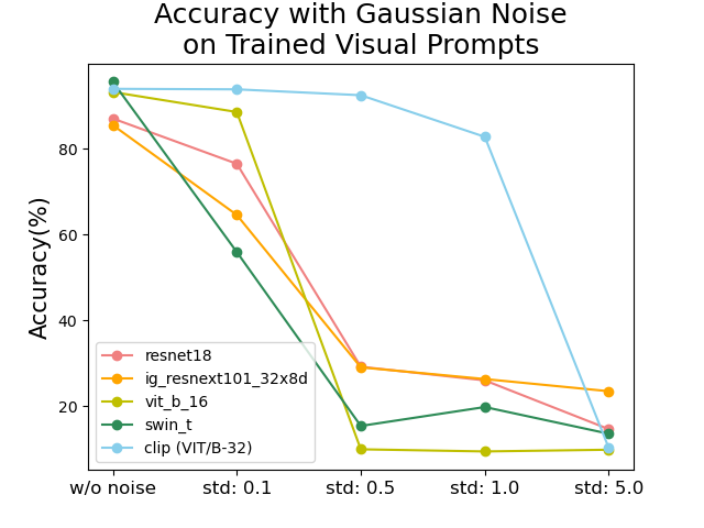
Figure 8: Accuracy Decline with Gaussian Noise. The figure illustrates the accuracy of SVHN across different models with varying levels of Gaussian noise (with a standard deviation ranging from 0.1 to 5.0) are added to the trained visual prompts.

In LogME You et al. (2021), the evidence score is used to rank the transfer performance of pre-trained models. However, this ranking may fail for the visual prompting framework because different models exhibit varying sensitivities to prompts. Fig. 8 illustrates the accuracy decline of different pre-trained models under various levels of Gaussian noise. As shown, when the noise standard deviation increases to 0.5, the accuracy of ViT-B-16 and Swin-t decreases sharply. This indicates that these models are highly sensitive to prompts and require accurate prompts for correct predictions. This result is also reflected in Fig.9, where ViT-B-16 and Swin-T fail to improve their evidence scores effectively with different simulated prompts. Consequently, their scores fall behind those of other models, making model ranking less effective. Therefore, within the visual prompting framework, we do not rank pre-trained models based on the given dataset. Instead, we compare VP and LP with the same pre-trained model for consistency. (see Section 3.1).

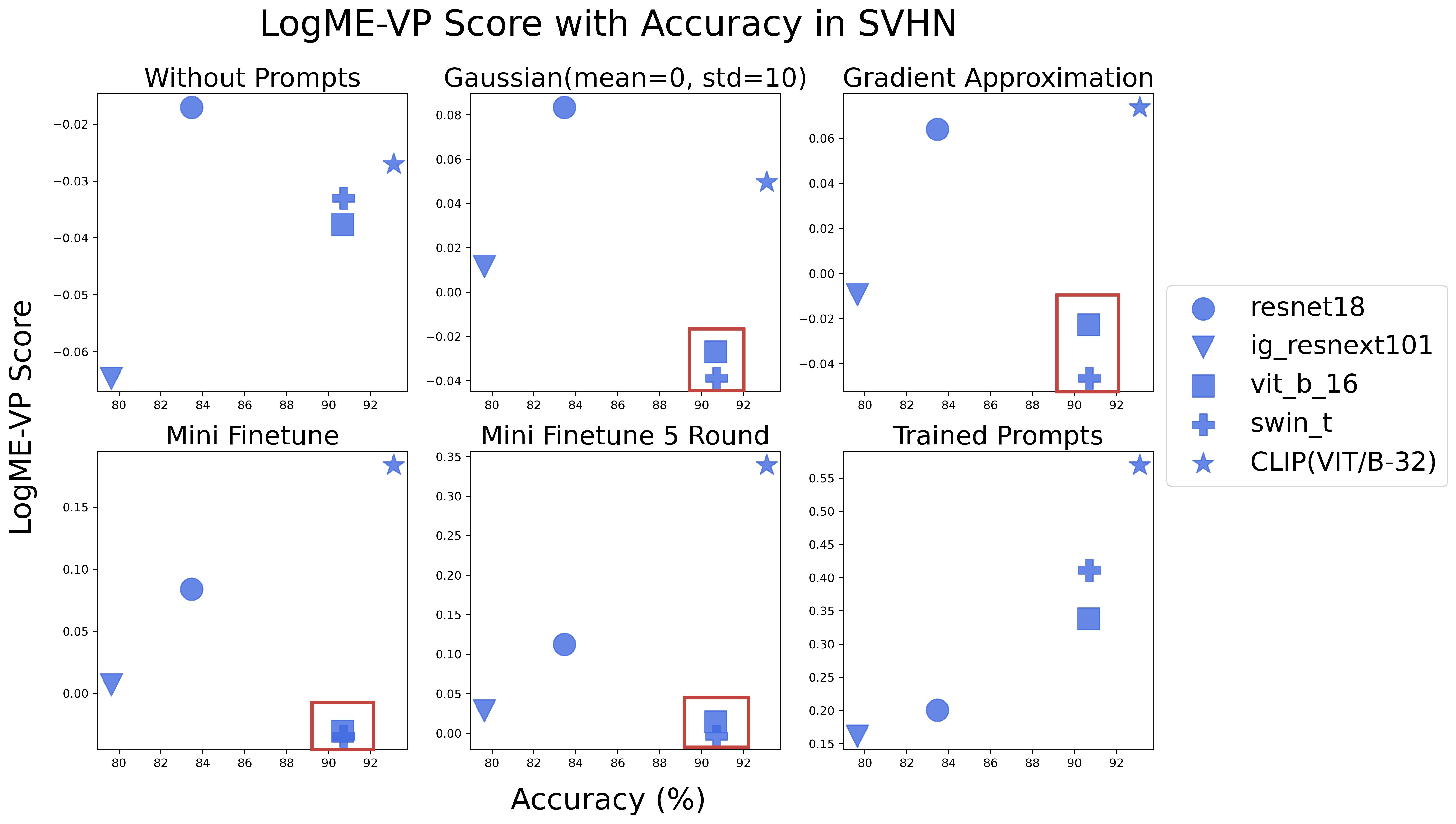
Figure 9: LogME-VP Score and Model Performance for SVHN. The LogME-VP score is computed across several visual prompt settings. The points enclosed in red frames highlight the pre-trained models that fall behind the overall trend.

References

- Bahng et al. (2022) Hyojin Bahng, Ali Jahanian, Swami Sankaranarayanan, and Phillip Isola. Exploring visual prompts for adapting large-scale models. arXiv preprint arXiv:2203.17274, 2022.
- Bishop and Nasrabadi (2006) Christopher M Bishop and Nasser M Nasrabadi. Pattern Recognition and Machine Learning (Information Science and Statistics). Springer-Verlag, Berlin, Heidelberg, 2006. ISBN 0387310738.
- Bossard et al. (2014) Lukas Bossard, Matthieu Guillaumin, and Luc Van Gool. Food-101 – mining discriminative components with random forests. In European Conference on Computer Vision, 2014.
- Chen et al. (2023) Aochuan Chen, Yuguang Yao, Pin-Yu Chen, Yihua Zhang, and Sijia Liu. Understanding and improving visual prompting: A label-mapping perspective. In Proceedings of the IEEE/CVF Conference on Computer Vision and Pattern Recognition, pages 19133–19143, 2023.
- Chen (2024) Pin-Yu Chen. Model reprogramming: Resource-efficient cross-domain machine learning. Proceedings of the AAAI Conference on Artificial Intelligence, 38(20):22584–22591, 2024.
- Christie et al. (2018) Gordon Christie, Neil Fendley, James Wilson, and Ryan Mukherjee. Functional map of the world. In Proceedings of the IEEE Conference on Computer Vision and Pattern Recognition, 2018.
- Cimpoi et al. (2014) M. Cimpoi, S. Maji, I. Kokkinos, S. Mohamed, , and A. Vedaldi. Describing textures in the wild. In Proceedings of the IEEE Conf. on Computer Vision and Pattern Recognition (CVPR), 2014.
- Codella et al. (2019) Noel Codella, Veronica Rotemberg, Philipp Tschandl, M Emre Celebi, Stephen Dusza, David Gutman, Brian Helba, Aadi Kalloo, Konstantinos Liopyris, Michael Marchetti, et al. Skin lesion analysis toward melanoma detection 2018: A challenge hosted by the international skin imaging collaboration (isic). arXiv preprint arXiv:1902.03368, 2019.
- Cohen et al. (2009) Israel Cohen, Yiteng Huang, Jingdong Chen, Jacob Benesty, Jacob Benesty, Jingdong Chen, Yiteng Huang, and Israel Cohen. Pearson correlation coefficient. Noise reduction in speech processing, pages 1–4, 2009.
- Dosovitskiy et al. (2020) Alexey Dosovitskiy, Lucas Beyer, Alexander Kolesnikov, Dirk Weissenborn, Xiaohua Zhai, Thomas Unterthiner, Mostafa Dehghani, Matthias Minderer, Georg Heigold, Sylvain Gelly, et al. An image is worth 16x16 words: Transformers for image recognition at scale. arXiv preprint arXiv:2010.11929, 2020.
- Elsayed et al. (2019) Gamaleldin F. Elsayed, Ian Goodfellow, and Jascha Sohl-Dickstein. Adversarial reprogramming of neural networks. In International Conference on Learning Representations, 2019. URL https://openreview.net/forum?id=Syx_Ss05tm.
- He et al. (2016) Kaiming He, Xiangyu Zhang, Shaoqing Ren, and Jian Sun. Deep residual learning for image recognition. In Proceedings of the IEEE conference on computer vision and pattern recognition, pages 770–778, 2016.
- Helber et al. (2019) Patrick Helber, Benjamin Bischke, Andreas Dengel, and Damian Borth. Eurosat: A novel dataset and deep learning benchmark for land use and land cover classification. IEEE Journal of Selected Topics in Applied Earth Observations and Remote Sensing, 2019.
- Hendrycks and Gimpel (2017) Dan Hendrycks and Kevin Gimpel. A baseline for detecting misclassified and out-of-distribution examples in neural networks. In International Conference on Learning Representations, 2017. URL https://openreview.net/forum?id=Hkg4TI9xl.
- Houben et al. (2013) Sebastian Houben, Johannes Stallkamp, Jan Salmen, Marc Schlipsing, and Christian Igel. Detection of traffic signs in real-world images: The german traffic sign detection benchmark. In The 2013 International Joint Conference on Neural Networks (IJCNN), pages 1–8, 2013.
- Hsiung et al. (2023) Lei Hsiung, Yung-Chen Tang, Pin-Yu Chen, and Tsung-Yi Ho. NCTV: Neural Clamping Toolkit and Visualization for Neural Network Calibration. In Proceedings of the Thirty-Seventh AAAI Conference on Artificial Intelligence. Association for the Advancement of Artificial Intelligence, February 2023.
- Jia et al. (2022) Menglin Jia, Luming Tang, Bor-Chun Chen, Claire Cardie, Serge Belongie, Bharath Hariharan, and Ser-Nam Lim. Visual prompt tuning. In European Conference on Computer Vision, pages 709–727. Springer, 2022.
- Kendall (1938) Maurice G Kendall. A new measure of rank correlation. Biometrika, 30(1-2):81–93, 1938.
- Krishnamachari et al. (2023) Kiran Krishnamachari, See-Kiong Ng, and Chuan-Sheng Foo. Fourier sensitivity and regularization of computer vision models. arXiv preprint arXiv:2301.13514, 2023.
- Krizhevsky and Hinton (2009) Alex Krizhevsky and Geoffrey Hinton. Learning multiple layers of features from tiny images. Technical report, University of Toronto, Toronto, Ontario, 2009.
- Kullback and Leibler (1951) Solomon Kullback and Richard A Leibler. On information and sufficiency. The annals of mathematical statistics, 22(1):79–86, 1951.
- Lee et al. (2018) Kimin Lee, Kibok Lee, Honglak Lee, and Jinwoo Shin. A simple unified framework for detecting out-of-distribution samples and adversarial attacks. Advances in neural information processing systems, 31, 2018.
- Liang et al. (2018) Shiyu Liang, Yixuan Li, and Rayadurgam Srikant. Enhancing the reliability of out-of-distribution image detection in neural networks. In International Conference on Learning Representations, 2018. URL https://openreview.net/forum?id=H1VGkIxRZ.
- Liu et al. (2021) Ze Liu, Yutong Lin, Yue Cao, Han Hu, Yixuan Wei, Zheng Zhang, Stephen Lin, and Baining Guo. Swin transformer: Hierarchical vision transformer using shifted windows. In Proceedings of the IEEE/CVF international conference on computer vision, pages 10012–10022, 2021.
- Mahajan et al. (2018) Dhruv Mahajan, Ross Girshick, Vignesh Ramanathan, Kaiming He, Manohar Paluri, Yixuan Li, Ashwin Bharambe, and Laurens Van Der Maaten. Exploring the limits of weakly supervised pretraining. In Proceedings of the European conference on computer vision (ECCV), pages 181–196, 2018.
- Netzer et al. (2011) Yuval Netzer, Tao Wang, Adam Coates, Alessandro Bissacco, Bo Wu, and Andrew Y Ng. Reading digits in natural images with unsupervised feature learning. NIPS Workshop on Deep Learning and Unsupervised Feature Learning, 2011.
- Nguyen et al. (2020) Cuong Nguyen, Tal Hassner, Matthias Seeger, and Cedric Archambeau. Leep: A new measure to evaluate transferability of learned representations. In International Conference on Machine Learning, pages 7294–7305. PMLR, 2020.
- Nilsback and Zisserman (2008) M-E. Nilsback and A. Zisserman. Automated flower classification over a large number of classes. In Proceedings of the Indian Conference on Computer Vision, Graphics and Image Processing, Dec 2008.
- Parkhi et al. (2012) Omkar M Parkhi, Andrea Vedaldi, Andrew Zisserman, and CV Jawahar. Cats and dogs. In 2012 IEEE conference on computer vision and pattern recognition, pages 3498–3505. IEEE, 2012.
- Radford et al. (2021) Alec Radford, Jong Wook Kim, Chris Hallacy, Aditya Ramesh, Gabriel Goh, Sandhini Agarwal, Girish Sastry, Amanda Askell, Pamela Mishkin, Jack Clark, et al. Learning transferable visual models from natural language supervision. In International conference on machine learning, pages 8748–8763. PMLR, 2021.
- Russakovsky et al. (2015) Olga Russakovsky, Jia Deng, Hao Su, Jonathan Krause, Sanjeev Satheesh, Sean Ma, Zhiheng Huang, Andrej Karpathy, Aditya Khosla, Michael Bernstein, Alexander C. Berg, and Li Fei-Fei. ImageNet Large Scale Visual Recognition Challenge. International Journal of Computer Vision (IJCV), 115(3):211–252, 2015.
- Soomro et al. (2012) Khurram Soomro, Amir Roshan Zamir, and Mubarak Shah. Ucf101: A dataset of 101 human actions classes from videos in the wild. arXiv preprint arXiv:1212.0402, 2012.
- Spearman (1904) C Spearman. The proof and measurement of association between two things. The American Journal of Psychology, 15(1):72–101, 1904.
- Tang et al. (2024) Yung-Chen Tang, Pin-Yu Chen, and Tsung-Yi Ho. Neural Clamping: Joint Input Perturbation and Temperature Scaling for Neural Network Calibration. Transactions on Machine Learning Research, 2024. ISSN 2835-8856. URL https://openreview.net/forum?id=qSFToMqLcq.
- Tran et al. (2019) Anh T Tran, Cuong V Nguyen, and Tal Hassner. Transferability and hardness of supervised classification tasks. In Proceedings of the IEEE/CVF International Conference on Computer Vision, pages 1395–1405, 2019.
- Tsai et al. (2020) Yun-Yun Tsai, Pin-Yu Chen, and Tsung-Yi Ho. Transfer learning without knowing: Reprogramming black-box machine learning models with scarce data and limited resources. In International Conference on Machine Learning, pages 9614–9624. PMLR, 2020.
- Tsao et al. (2024) Hsi-Ai Tsao, Lei Hsiung, Pin-Yu Chen, Sijia Liu, and Tsung-Yi Ho. AutoVP: An automated visual prompting framework and benchmark. In The Twelfth International Conference on Learning Representations, 2024. URL https://openreview.net/forum?id=wR9qVlPh0P.
- Tschandl et al. (2018) Philipp Tschandl, Cliff Rosendahl, and Harald Kittler. The ham10000 dataset, a large collection of multi-source dermatoscopic images of common pigmented skin lesions. Scientific data, 5(1):1–9, 2018.
- You et al. (2021) Kaichao You, Yong Liu, Jianmin Wang, and Mingsheng Long. Logme: Practical assessment of pre-trained models for transfer learning. In International Conference on Machine Learning, pages 12133–12143. PMLR, 2021.
- Zhang et al. (2020) Chaoning Zhang, Philipp Benz, Tooba Imtiaz, and In So Kweon. Understanding adversarial examples from the mutual influence of images and perturbations. In Proceedings of the IEEE/CVF Conference on Computer Vision and Pattern Recognition, pages 14521–14530, 2020.