Frugal RIS-aided 3D Localization with CFO under LoS and NLoS Conditions

Abstract

In this paper, we investigate 3-D localization and frequency synchronization with multiple reconfigurable intelligent surfaces in the presence of carrier frequency offset (CFO) for a stationary user equipment (UE). In line with the 6G goals of sustainability and efficiency, we focus on a frugal communication scenario with minimal spatial and spectral resources (i.e., narrowband single-input single-ouput system), considering both the presence and blockage of the line-of-sight (LoS) path between the base station (BS) and the UE. We design a generalized likelihood ratio test (GLRT)-based LoS detector, channel parameter estimation and localization algorithms, with varying complexity. To verify the efficiency of our estimators, we compare the root mean-squared error (RMSE) to the Cramér-Rao bound (CRB) of the unknown parameters. We also evaluate the sensitivity of our algorithms to the presence of uncontrolled multi-path components (MPC) and various levels of CFO. Simulation results showcase the effectiveness of the proposed algorithms under minimal hardware and spectral requirements, and a wide range of operating conditions, thereby confirming the viability of RIS-aided frugal localization in 6G scenarios.

I Introduction

Accurate positioning is a pre-requisite for many modern use-cases, finding applications in various areas such as autonomous driving, augmented reality, navigation, etc. [1]. While Global Positioning System (GPS) stands out as the ubiquitous solution for navigation, its efficacy is often compromised in scenarios where a direct line of sight to satellites is obstructed, such as in tunnels, dense urban environments and indoors. An alternative solution is to use cellular networks. Cellular networks have been used for positioning since the first generation (1G) of mobile networks [2]. In 4G networks, time-difference-of-arrival (TDoA) and angle-of-arrival (AoA)-based techniques were introduced, which rely on multiple base stations to estimate the position of a mobile device. These techniques proved to be more accurate than the previous ones, but required additional infrastructure and were not suitable for indoor environments. In 5G networks, the adoption of mmWave frequencies and beamforming techniques improved the accuracy of positioning [3, 4, 5]. In 6G networks, the use of RISs is expected to further enhance the accuracy and reliability of cellular-based localization [6, 7, 8, 9].

In advancement of wireless communications through successive generations, achieving sustainability and improving energy and spectral efficiency has always been a central objective, and the upcoming 6G is no exception [10]. As pointed out, 4G networks succeeded in improving positioning by putting a minimum requirement on hardware resources and 5G managed to progress further in positioning by accessing large chunks of bandwidth in mmWave and large antenna arrays. Therefore, the question remains whether 6G will continue this trend or if there could be another solution to achieve improved positioning without leveraging more resources. The use of RISs appears to be a key point in this regard.

RISs constitute one of the key-technology enablers for 6G [11], providing an additional, controllable path between the BS and the UE. Primarily, RISs are designed as a cost-effective and energy-efficient solution to address signal blockage challenges without the need to densify the network with more BSs. This approach is favored due to the simpler hardware requirements and lower maintenance costs associated with RIS [12], [13]. RISs consist of a large number of small elements that can be manipulated to reflect incident waves in desired directions [14]. Deploying RISs in an environment allows for the engineering of the propagation medium, enhancing signal strength and reducing interference at targeted locations [15]. This ultimately enhances communication rate and coverage [16] while providing significant gains in localization performance [17].

The use of RISs in radio localization has been extensively studied in the literature, with numerous works exploring the potential of RISs to improve UE localization thanks to the additional reflected paths. Notable contributions include [6, 18, 19], which discuss the challenges, opportunities, and research directions related to RIS-aided positioning. Since localization often comes as a by-product of cellular communication systems, it is advantageous if it is frugal with resources, such as antennas and time-frequency allocations, to avoid compromising the quality and infrastructure requirements of wireless communications—so far the primary objective of cellular networks. Along this line, RIS-based narrowband (NB) localization was discussed in [20], where a NB RIS-based multiple-input single-output (MISO) localization approach for a single-antenna UE was investigated. RIS-enabled localization with single BS and single antenna is discussed in [21, 22]. In [21], a localization and clock-synchronization approach to single-input single-output (SISO), single RIS wideband (WB) case was introduced. In [22], authors propose a method for single-antenna receiver 2-D localization and achieve centimeter-level localization accuracy with fingerprinting the RIS-phases over time. A broader perspective on frugal localization was taken in [23], which conducted an analysis on UE localization scenarios with minimal required number of BS and RISs, showing that it is possible to estimate the UE’s position with one BS and two RISs under NB communication even without a direct path from the BS to the UE.

A common weakness in the above works is that they ignore the presence of CFO between the BS and the UE. Since both CFO and the use of diverse RIS phase profiles [24] (i.e., beam sweeping for angle-of-departure (AoD) estimation from the RIS using beamspace measurements at the UE [25, 20]) over time lead to phase variations across consecutive transmissions, the impacts of CFO and RIS profile variation add up together in the time-series of phase shifts, resulting in the so-called angle-Doppler/CFO coupling effect, as noted in [26, 27]. From an experimental perspective, [23] demonstrates SISO localization of a stationary UE with one BS and two RISs in the absence of a CFO. However, this study has the impractical requirement that the BS and UE share a common oscillator to eliminate CFO issues. Moreover, the approach relies on using directional RIS beams to sweep potential locations and estimate AoDs from the RISs. This method is ineffective with random RIS phase profiles, which are commonly used in RIS-aided communications when UE locations are unknown, e.g., [28, 29, 30]. Overall, no systematic study has been conducted to address the problem of frugal localization and frequency synchronization with the help of RISs under angle/CFO coupling effect and when employing random RIS phase configurations. Therefore, in light of the existing literature, two crucial questions emerge that remain unanswered: (i) is it possible to perform joint 3-D downlink localization and frequency synchronization in the challenging SISO NB (i.e., single-carrier) scenario with multiple RISs employing random phase configurations?; and (ii) can efficient and low-complexity algorithms be developed for LoS presence detection, channel parameter/CFO estimation and localization in both the presence and absence of the direct LoS path between the BS and the UE?

In an attempt to address the identified shortcomings of existing studies on RIS-aided localization and fill the corresponding research gaps, we consider the frugal localization problem of a UE in case of NB SISO signaling via one BS and several RISs employing random phase profiles. The novel contributions of this paper can be summarized as follows.

• Frugal localization under CFO: We formalize the problem of NB RIS-aided SISO localization and frequency synchronization under the assumption of CFO between the transmitter and the receiver with parsimonious usage of resources. We develop novel low-complexity estimators of the unknowns, including the CFO and AoDs, which enable us to perform localization. Different estimation algorithms under various circumstances are designed, including one estimation algorithm in case the direct LoS between the BS and the UE is present, as well as two estimation algorithms in case of blocked LoS between the BS and UE. Our estimators achieve the theoretical bounds at moderate to high transmit power. Simulation results show the efficiency of the estimator with respect to theoretical bounds.

• LoS detection: We design a GLRT-based detector to determine if the LoS exists or not, which complements the above contribution to a full localization and synchronization algorithm. Our proposed algorithm is capable of attaining the theoretical bounds at a moderate to high transmit power.

• Sensitivity analysis: We assess the sensitivity of our algorithm to MPC, which shows that our algorithm quickly converges to the achievable bounds with Rician factor as small as $10$. We also study the sensitivity of CFO estimation on the overall performance of our algorithm by ignoring CFO as an unknown. The performance drastically deteriorates at CFO values much smaller than values typically found in UE, suggesting the importance of accurate estimation of the CFO.

• Resource Efficiency: We prove that with a minimalistic hardware/spectral configuration, including a single antenna and single subcarrier and sufficient number of RISs, it is possible to perform accurate positioning. Therefore, our approach sets a new benchmark for resource efficiency in communication systems, potentially reducing the cost and complexity of deployment, which is in accordance with 6G objectives.

The paper is structured as follows. In Sec. II, the system setup is detailed. Sec. III describes orthogonal RIS profile design to facilitate per-RIS AoD and CFO estimation. Sec. IV describes the overall flow of the algorithm, including channel parameter estimation under LoS and non-line-of-sight (NLoS), localization under LoS and NLoS, and detection of if the LoS is present or not. Channel parameter turns out to be the main challenge and low-complexity methods are derived in Sec. V: in Sec. V-A, estimation algorithms in case the direct link between the BS and UE (LoS) exists will be explained. Sec. V-B sheds light on estimation algorithms in the more challenging scenario in which the LoS path does not exist.

Notation

Vectors and matrices are shown by bold-face lower-case and bold-face upper-case letters respectively. The notations $(.)^{\mathsf{T}}$ and $(.)^{\mathsf{H}}$ indicate transpose and hermitian transpose. All one vector with size $n$ denoted by $\bm{1}_{n}$ and the identity matrix with size $n$ is represented by $\mathbf{I}_{n}$. The L2 norm of a vector is shown by $\left\lVert.\right\rVert$. The matrix $\bm{R}_{z}(\theta)$ denotes the 3-D rotation matrix by an angle $\theta$ about the z-axis. The Kronecker product and the Hadamard product are shown by $\otimes$ and $\odot$ respectively.

II System Model

In this section, we describe the proposed localization system that promotes the parsimonious use of spatial and spectral resources for joint location and frequency offset estimation of a static user.

II-A Scenario

Consider a RIS-aided downlink (DL) localization system with a single-antenna BS, $R$ identical $N$-element RISs, and a single-antenna UE, as shown in Fig. 1. The BS and the RISs are located at known positions $\bm{p}_{\text{BS}}\in\mathbb{R}^{3}$ and $\bm{p}_{{\text{RIS}},r}\in\mathbb{R}^{3}$, $r=1,\cdots,R$ (denoting the RIS centers) respectively, while the UE has an unknown position $\bm{p}\in\mathbb{R}^{3}$. The RISs are assumed to have known orientations, represented by the unitary rotation matrices $\bm{R}_{r}\in\text{SO}(3)\subset\mathbb{R}^{3\times 3}$, $r=1,\cdots,R$, that map the global frame of reference to the local coordinate systems of the RISs. The UE is considered stationary. Moreover, due to oscillator inaccuracies, the UE is not perfectly frequency-synchronized to the BS, which leads to an unknown CFO $\nu\in\mathbb{R}$ at the UE with respect to the BS [31, 32].

II-B Geometric Relations

The AoD from the ${r^{\rm{th}}}$ RIS to the UE is denoted by $\bm{\theta}_{r}=\big{[}[\bm{\theta}_{r}]_{\rm{az}},[\bm{\theta}_{r}]_{\rm{el}}\big{]}^{\mathsf{T}}\in\mathbb{R}^{2}$, where

$$[\bm{\theta}_{r}]_{\rm{az}} =\operatorname{\mathrm{atan2}}\left([\bm{r}_{r}]_{2},[\bm{r}_{r}]_{1}\right),$$ (1)

$$[\bm{\theta}_{r}]_{\rm{el}} =\arccos\left(\frac{[\bm{r}_{r}]_{3}}{\left\lVert\bm{p}-\bm{p}_{{\text{RIS}},r}\right\rVert}\right),$$ (2)

with $\bm{r}_{r}=\bm{R}_{r}(\bm{p}-\bm{p}_{{\text{RIS}},r})$ representing the vector extending from the ${r^{\rm{th}}}$ RIS to the UE in the local frame of reference of the ${r^{\rm{th}}}$ RIS.

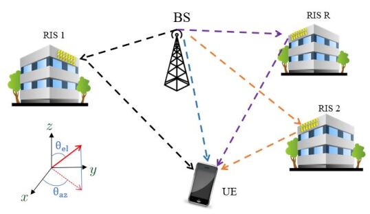
Figure 1: Frugal localization scenario involving one single-antenna BS, $R$ RISs and one single-antenna user with NB (single-carrier) communication.

II-C Signal Model

The BS transmits NB pilot symbols $\bm{s}=[s_{0}\,\cdots\,s_{M-1}]^{\mathsf{T}}\in\mathbb{C}^{M}$ over $M$ transmission instances with sampling period $T_{s}$ and a power constraint $\left\lVert\bm{s}\right\rVert^{2}=MP$. Assuming the absence of uncontrolled multipath (i.e., due to reflection or scattering off passive objects) as in [21, 28, 33, 34, 20], the received complex baseband signal at the UE associated to the ${m^{\rm{th}}}$ transmission is given by

$$y_{m}=h_{m}e^{j2\pi mT_{s}\nu}s_{m}+n_{m},$$ (3)

where $T_{s}\in\mathbb{R}$ is the symbol duration, the term $e^{j2\pi mT_{s}\nu}$ results from the CFO between the BS and the UE, $n_{m}\in\mathbb{C}$ denotes circularly symmetric complex Gaussian noise with $n_{m}\sim{\mathcal{CN}}(0,\sigma^{2})$, and $h_{m}\in\mathbb{C}$ represents the overall BS-UE channel for the ${m^{\rm{th}}}$ transmission involving both the LoS path and the NLoS paths through the RISs, i.e.,

$$h_{m}=h_{{\text{LoS}},m}+h_{{\text{RIS}},m}.$$ (4)

In (4), $h_{{\text{LoS}},m}\in\mathbb{C}$ is the LoS (i.e., direct) channel between the BS and the UE, written as

$$h_{{\text{LoS}},m}=\alpha_{0},$$ (5)

where $\alpha_{0}\in\mathbb{C}$ denotes the channel gain. As to the NLoS channel in (4), it can be defined as

$$h_{{\text{RIS}},m}=\sum_{r=1}^{R}\alpha_{r}\,\bm{a}^{\mathsf{T}}(\bm{\theta}_{r})\mathrm{diag}(\bm{\gamma}_{r,m})\bm{a}(\bm{\phi}_{r}),$$ (6)

where $\alpha_{r}\in\mathbb{C}$ is the channel gain over the BS-(${r^{\rm{th}}}$ RIS)-UE path and $\bm{\phi}_{r}\in\mathbb{R}^{2}$ denotes the known AoA from the BS at the ${r^{\rm{th}}}$ RIS (given the known positions and orientations of the BS and the RISs). In addition, $\bm{\gamma}_{r,m}\in\mathbb{C}^{N}$ represents the phase profile of the ${r^{\rm{th}}}$ RIS at time $m$ and $\bm{a}(\cdot)\in\mathbb{C}^{N}$ is the RIS steering vector, given by [21]

$$[\bm{a}(\bm{\psi})]_{n}=\exp\left(j\bm{k}^{\mathsf{T}}(\bm{\psi})\bm{q}_{n}\right),$$ (7)

for a generic $\bm{\psi}$ where $\bm{q}_{n}\in\mathbb{R}^{3}$ denotes the known position of the ${n^{\rm{th}}}$ RIS element with respect to the RIS center in the local coordinate system of the RIS, and

$$\bm{k}(\bm{\psi})=\frac{2\pi}{\lambda}$$ (8)

$$\left[\sin([\bm{\psi}]_{\rm{el}})\cos([\bm{\psi}]_{\rm{az}}),\,\sin([\bm{\psi}]_{\rm{el}})\sin([\bm{\psi}]_{\rm{az}}),\,\cos([\bm{\psi}]_{\rm{el}})\right]^{\mathsf{T}}$$

is the wavenumber vector defined for a given angle $\bm{\psi}$. Let

$$\bm{W}_{r} \triangleq[\bm{a}(\bm{\phi}_{r})\odot\bm{\gamma}_{r,0}\leavevmode\nobreak\ \cdots\leavevmode\nobreak\ \bm{a}(\bm{\phi}_{r})\odot\bm{\gamma}_{r,M-1}]\in\mathbb{C}^{N\times M},$$ (9)

$$\bm{b}(\nu) \triangleq[1\leavevmode\nobreak\ e^{j2\pi T_{s}\nu}\leavevmode\nobreak\ \cdots\leavevmode\nobreak\ e^{j2\pi(M-1)T_{s}\nu}]^{\mathsf{T}}\in\mathbb{C}^{M}.$$ (10)

Then, using (4)–(6) and (9)–(10), the aggregated observations in (3) over $M$ transmissions can be written as

$$\bm{y}=\sqrt{P}\Big{(}\alpha_{0}\,\bm{b}(\nu)+\sum_{r=1}^{R}\alpha_{r}\,\bm{x}_{r}(\bm{\theta}_{r})\odot\bm{b}(\nu)\Big{)}+\bm{n},$$ (11)

where $\bm{y}\triangleq[y_{0}\,\cdots\,y_{M-1}]^{\mathsf{T}}\in\mathbb{C}^{M}$, $\bm{x}_{r}(\bm{\theta}_{r})=\bm{W}_{r}^{\mathsf{T}}\bm{a}(\bm{\theta}_{r})$ and $\bm{n}\in\mathbb{C}^{M}$ is the noise component with $\bm{n}\sim{\mathcal{CN}}({{\bm{0}}},\sigma^{2}{\bm{\mathrm{I}}})$. In (11), we have set $s_{m}=\sqrt{P},\,\forall m$ for simplicity.

II-D Joint Localization and Frequency Synchronization Problem

The goal is to estimate the position $\bm{p}$ and the CFO $\nu$ of the UE from the observation $\bm{y}$ in (11). For this estimation problem, the unknown channel-domain parameters are given by

$$\bm{\eta}_{\rm{ch}}=[\alpha_{{\rm{R}},0}\leavevmode\nobreak\ \alpha_{{\rm{I}},0}\leavevmode\nobreak\ \cdots\leavevmode\nobreak\ \alpha_{{\rm{R}},R}\leavevmode\nobreak\ \alpha_{{\rm{I}},R}\leavevmode\nobreak\ \nu\leavevmode\nobreak\ \bm{\theta}_{1}^{\mathsf{T}}\leavevmode\nobreak\ \cdots\leavevmode\nobreak\ \bm{\theta}_{R}^{\mathsf{T}}]\in\mathbb{R}^{4R+3},$$ (12)

while the location-domain unknown parameter vector is

$$\bm{\eta}=[\alpha_{{\rm{R}},0}\leavevmode\nobreak\ \alpha_{{\rm{I}},0}\leavevmode\nobreak\ \cdots\leavevmode\nobreak\ \alpha_{{\rm{R}},R}\leavevmode\nobreak\ \alpha_{{\rm{I}},R}\leavevmode\nobreak\ \nu\leavevmode\nobreak\ \bm{p}^{\mathsf{T}}]^{\mathsf{T}}\in\mathbb{R}^{2R+6}.$$ (13)

Here, $\alpha_{{\rm{R}},r}\triangleq\Re\left\{\alpha_{r}\right\}$ and $\alpha_{{\rm{I}},r}\triangleq\Im\left\{\alpha_{r}\right\}$, $r=0,\cdots,R$. Clearly, in case no LoS exists between the UE and the BS, the channel-domain vector and the location-domain vector would change into $\bm{\eta}_{\rm{ch}}=[\alpha_{{\rm{R}},1}\leavevmode\nobreak\ \alpha_{{\rm{I}},1}\leavevmode\nobreak\ \cdots\leavevmode\nobreak\ \alpha_{{\rm{R}},R}\leavevmode\nobreak\ \alpha_{{\rm{I}},R}\leavevmode\nobreak\ \nu\leavevmode\nobreak\ \bm{\theta}_{1}^{\mathsf{T}}\leavevmode\nobreak\ \cdots\leavevmode\nobreak\ \bm{\theta}_{R}^{\mathsf{T}}]\in\mathbb{R}^{4R+1},$ and $\bm{\eta}=[\alpha_{{\rm{R}},1}\leavevmode\nobreak\ \alpha_{{\rm{I}},1}\leavevmode\nobreak\ \cdots\leavevmode\nobreak\ \alpha_{{\rm{R}},R}\leavevmode\nobreak\ \alpha_{{\rm{I}},R}\leavevmode\nobreak\ \nu\leavevmode\nobreak\ \bm{p}^{\mathsf{T}}]^{\mathsf{T}}\in\mathbb{R}^{2R+4},$ respectively.

It should be noted that the LoS path does not directly convey positional information because the UE’s position is a function of the AoDs according to (1)–(2). However, as we will see in Sec. VI, the accuracy of CFO estimation is improved if the LoS is present, and as a result, the residual error in RIS path separation decreases as discussed in Sec. III, simplifying also the AoD estimation algorithm.

III RIS Profile Design

Estimating the channel-domain parameters in (12) requires a complex high-dimensional optimization, which is cumbersome even in the case of $R=2$. To circumvent this, we leverage the controllability offered by the RIS by designing an orthogonal temporal-coding for RIS phase profiles [35]. In the absence of CFO, the contributions from $R+1$ paths in (11) can be separated and the unknowns from each RIS path can be estimated separately.

III-A Hadamard-based Design

The idea involves using the rows of the Hadamard matrix to encode the phase profiles of the RISs, followed by a simple post processing at the receiver to retrieve the contributions from each path [35].

We first divide the total transmissions into $L\geq 2^{\lceil{\log_{2}(R+1)}\rceil}$ equal-sized blocks. Choose $L$ such that it is a factor of $M$. We next define $\bm{P}_{r}\in\mathbb{C}^{N\times(M/L)}$, $r=1,\cdots,R$ as a set of base phase profiles of length $M/L$ for each RIS. These profiles may be random in case there is no prior information about the UE location, or directional in case partial information about the UE location is available.

We take $R$ rows of the Hadamard matrix of length $L$ (except for the first row, which is constant) as the coding vectors $\mathbf{c}_{r}\in\mathbb{R}^{L}$ for the ${r^{\rm{th}}}$ RIS. Then we then form the full phase profile of each RIS at transmission $m=kL+l$

$$\bm{\gamma}_{r,kL+l}=\left([\mathbf{c}_{r}]_{l}\right){\bm{P}_{r}}_{[:,k]},$$ (14)

where ${\bm{P}_{r}}_{[:,k]}$ denotes the ${k^{\rm{th}}}$ column of $\bm{P}_{r}$, $k=0,\cdots,M/L-1$ and $l=0,\cdots,L-1$.

At the receiver side, to extract the ${r^{\rm{th}}}$ RIS components from (11), it is enough to reshape the received signal $\bm{y}\in\mathbb{C}^{M}$ as

$$\mathbf{Y}=[\bm{y}_{0:L-1}|\bm{y}_{L:2L-1}|\cdots|\bm{y}_{M-L:M-1}]\in\mathbb{C}^{L\times(M/L)},$$ (15)

and then compute

$$\bm{y}_{r}=\frac{1}{L}\mathbf{Y}^{\mathsf{T}}\mathbf{c}_{r},\leavevmode\nobreak\ r=1,\cdots,R.$$ (16)

where $\bm{y}_{r}\in\mathbb{C}^{M/L}$ is the filtered signal containing the ${r^{\rm{th}}}$ RIS components. It is possible to separate the LoS component using $\bm{y}_{0}={1}/{L}\mathbf{Y}^{\mathsf{T}}\mathbf{c}_{0},$ where $\mathbf{c}_{0}=\bm{1}_{L}$.

III-B Example

As an example, we fix the number of RISs to $R=2$. Note that to separate the contributions from the three paths (LoS, RIS 1 and RIS 2), the minimum required coding length is $L=4$. We take $\mathbf{c}_{0}=[1,1,1,1]^{\mathsf{T}}$, $\mathbf{c}_{1}=[1,-1,1,-1]^{\mathsf{T}}$ and $\mathbf{c}_{2}=[1,1,-1,-1]^{\mathsf{T}}$. Then we can write the $4$ consecutive noise-free samples of $\bm{z}_{0}=\sqrt{P}\alpha_{0}\,\bm{b}(\nu)$ and $\bm{z}_{r}=\sqrt{P}\alpha_{r}\,\bm{x}_{r}(\bm{\theta}_{r})\odot\bm{b}(\nu)$, $r=1,2$ and $i=0,1,2,3$ as below

$$[\bm{z}_{0}]_{4k+i}=\sqrt{P}\alpha_{0}e^{j2\pi(4k+i)T_{s}\nu},$$ (17)

$$[\bm{z}_{1}]_{4k+i}=\sqrt{P}\alpha_{1}\left(\mathbf{c}_{r}(i)g_{1}(\bm{\phi}_{1},\bm{\theta}_{1},k)\right)e^{j2\pi(4k+i)T_{s}\nu},$$ (18)

$$[\bm{z}_{2}]_{4k+i}=\sqrt{P}\alpha_{2}\left(\mathbf{c}_{2}(i)g_{2}(\bm{\phi}_{2},\bm{\theta}_{2},k)\right)e^{j2\pi(4k+i)T_{s}\nu},$$ (19)

where $g_{r}(\bm{\phi}_{r},\bm{\theta}_{r},k)=(\bm{a}(\phi_{r})\odot{\bm{P}_{r}}_{[:,k]})^{\mathsf{T}}\bm{a}(\bm{\theta}_{r})$, $r=1,2$. Then, by applying (16) and in the case of $\nu=0$, the filtered measurements $\bm{y}_{0}$, $\bm{y}_{2}$ and $\bm{y}_{2}$ will be as follows

$$[\bm{y}_{0}]_{k}={\sqrt{P}}\alpha_{0}+[\tilde{\bm{n}}_{0}]_{k},$$ (20)

$$[\bm{y}_{1}]_{k}={\sqrt{P}}\alpha_{1}g_{1}(\bm{\phi}_{1},\bm{\theta}_{1},k)+[\tilde{\bm{n}}_{1}]_{k},$$ (21)

$$[\bm{y}_{2}]_{k}={\sqrt{P}}\alpha_{2}g_{2}(\bm{\phi}_{2},\bm{\theta}_{2},k)+[\tilde{\bm{n}}_{2}]_{k},$$ (22)

where $[\tilde{\bm{n}}_{r}]_{k}={1}/{4}\sum_{i=0}^{3}\mathbf{c}_{r}(i)[\bm{n}]_{4k+i}$ (see App. A). Therefore, $\bm{y}_{r}$, $r=1,2$ contain the contribution from the ${r^{\rm{th}}}$ RIS and $\bm{y}_{0}$ contain the LoS contribution without any interference from the other RISs. However, if $\nu\neq 0$, this coding would result in some residual inter-RIS interference and the separation cannot be done perfectly. The solution is to first estimate the CFO ($\hat{\nu}$) and remove it from the observations by $\tilde{\bm{y}}=\bm{y}\odot\bm{b}(-\hat{\nu})$, then proceed with this coding. Hence in the following sections, we proceed with estimating the CFO and cancel it out from the received signal.

IV High-level Algorithm Description

In this section, we provide a high-level description of the proposed joint localization and synchronization algorithm to tackle the problem in Sec. II-D, covering both the channel-domain parameter estimation and localization.

IV-A Channel-domain Parameter Estimation

The maximum-likelihood (ML) estimate of the channel-domain parameters from (11) can be obtained by solving the following optimization problems:

$$[\hat{\nu},\hat{\bm{\theta}}_{1},\cdots,\hat{\bm{\theta}}_{R},\hat{\alpha}_{0},\hat{\alpha}_{1},\cdots,\hat{\alpha}_{R}]=$$ (23)

$$\operatorname*{arg\,min}_{\begin{subarray}{c}\nu,\bm{\theta}_{1},\cdots,\bm{\theta}_{R},\\ \alpha_{0},\alpha_{1},\cdots,\alpha_{R}\end{subarray}}\big{\lVert}\bm{y}-\sqrt{P}\alpha_{0}\bm{b}(\nu)-\sqrt{P}\sum_{r=1}^{R}\alpha_{r}\bm{x}_{r}(\bm{\theta}_{r})\odot\bm{b}(\nu)\big{\rVert}^{2}\,,$$

if LoS exists, which we will refer to as LoS (with LoS) scenario, and

$$[\hat{\nu},\hat{\bm{\theta}}_{1},\cdots,\hat{\bm{\theta}}_{R},\hat{\alpha}_{1},\cdots,\hat{\alpha}_{R}]=$$ (24)

$$\operatorname*{arg\,min}_{\begin{subarray}{c}\nu,\bm{\theta}_{1},\cdots,\bm{\theta}_{R}\\ \alpha_{1},\cdots,\alpha_{R}\end{subarray}}\big{\lVert}\bm{y}-\sqrt{P}\sum_{r=1}^{R}\alpha_{r}\bm{x}_{r}(\bm{\theta}_{r})\odot\bm{b}(\nu)\big{\rVert}^{2}\,,$$

if LoS is blocked, which we will refer to as NLoS (no-LoS) scenario.

IV-A1 Conditional Channel Gain Estimation

The ML estimate of the path gains can be derived easily in closed-form as a function of the estimated CFO and AoDs as follows. First, we start by writing the received signal in the below form

$$\bm{y}=\bm{A}(\bm{\chi}_{\text{ch}})\bm{\alpha}+\bm{n},$$ (25)

where $\bm{\chi}_{\text{ch}}=[\nu,\bm{\theta}_{1}^{\mathsf{T}},\cdots,\bm{\theta}_{R}^{\mathsf{T}}]^{\mathsf{T}}$, $\bm{A}(\bm{\chi}_{\text{ch}})=\sqrt{P}[\bm{b}(\nu)\leavevmode\nobreak\ \leavevmode\nobreak\ \bm{x}_{1}(\bm{\theta}_{1})\odot\bm{b}(\nu)\leavevmode\nobreak\ \leavevmode\nobreak\ \cdots\leavevmode\nobreak\ \leavevmode\nobreak\ \bm{x}_{R}(\bm{\theta}_{R})\odot\bm{b}(\nu)]$ and $\bm{\alpha}=[\alpha_{0}\leavevmode\nobreak\ \alpha_{1}\leavevmode\nobreak\ \cdots\leavevmode\nobreak\ \alpha_{R}]^{\mathsf{T}},$ in case LoS exists and $\bm{A}(\bm{\chi}_{\text{ch}})=\sqrt{P}[\bm{x}_{1}(\bm{\theta}_{1})\odot\bm{b}(\nu)\leavevmode\nobreak\ \leavevmode\nobreak\ \cdots\leavevmode\nobreak\ \leavevmode\nobreak\ \bm{x}_{R}(\bm{\theta}_{R})\odot\bm{b}(\nu)]$ and $\bm{\alpha}=[\alpha_{1}\leavevmode\nobreak\ \cdots\leavevmode\nobreak\ \alpha_{R}]^{\mathsf{T}}$ in case LoS is blocked. Accordingly, the path gains can be estimated in closed-form as

$$\hat{\bm{\alpha}}(\bm{\chi}_{\text{ch}})=(\bm{A}(\bm{\chi}_{\text{ch}})^{\mathsf{H}}\bm{A}(\bm{\chi}_{\text{ch}}))^{-1}\bm{A}(\bm{\chi}_{\text{ch}})^{\mathsf{H}}\bm{y}.$$ (26)

IV-A2 Compressed Channel Parameter Estimation

We can now plug the channel gain estimates in (26) back into (23) and (24) to derive the compressed ML cost functions, reducing their dimensionality to $(2R+1)$ (which, however, still lead to very high computational complexity):

$$[\hat{\nu},\hat{\bm{\theta}}_{1},\cdots,\hat{\bm{\theta}}_{R}]=\operatorname*{arg\,min}_{\nu,\bm{\theta}_{1},\cdots,\bm{\theta}_{R}}$$ (27)

$$\big{\lVert}\bm{y}-\sqrt{P}\hat{\alpha}_{0}(\bm{\chi}_{\text{ch}})\bm{b}(\nu)-\sqrt{P}\sum_{r=1}^{R}\hat{\alpha}_{r}(\bm{\chi}_{\text{ch}})\bm{x}_{r}(\bm{\theta}_{r})\odot\bm{b}(\nu)\big{\rVert}^{2}.$$

in case LoS exists, and

$$[\hat{\nu},\hat{\bm{\theta}}_{1},\cdots,\hat{\bm{\theta}}_{R}]=$$ (28)

$$\operatorname*{arg\,min}_{\nu,\bm{\theta}_{1},\cdots,\bm{\theta}_{R}}\big{\lVert}\bm{y}-\sqrt{P}\sum_{r=1}^{R}\hat{\alpha}_{r}(\bm{\chi}_{\text{ch}})\bm{x}_{r}(\bm{\theta}_{r})\odot\bm{b}(\nu)\big{\rVert}^{2}.$$

in case LoS is bloked.

As discussed in Sec. III, it is possible to significantly simplify the optimization problems (27) and (28) with time-orthogonal RIS phase profiles, assuming a good estimate of the CFO is available. Sec. V will provide a detailed explanation of how to solve these two optimization problems with reasonable complexity, leveraging the orthogonal RIS profile design.

IV-B Localization

The direct ML approach to solve the localization and synchronization problem in in Sec. II-D is as follows:

$$[\hat{\nu},\leavevmode\nobreak\ \hat{\bm{p}}]=\operatorname*{arg\,min}_{\nu,\bm{p}}\big{\lVert}\bm{y}-$$

$$\sqrt{P}\hat{\alpha}_{0}(\bm{\chi}_{\text{p}})\bm{b}(\nu)-\sqrt{P}\sum_{r=1}^{R}\hat{\alpha}_{r}(\bm{\chi}_{\text{p}})\bm{x}_{r}(\bm{p})\odot\bm{b}(\nu)\big{\rVert}^{2},$$ (29)

in LoS scenario, and

$$[\hat{\nu},\leavevmode\nobreak\ \hat{\bm{p}}]=\operatorname*{arg\,min}_{\nu,\bm{p}}\big{\lVert}\bm{y}-\sqrt{P}\sum_{r=1}^{R}\hat{\alpha}_{r}(\bm{\chi}_{\text{p}})\bm{x}_{r}(\bm{p})\odot\bm{b}(\nu)\big{\rVert}^{2},$$ (30)

in NLoS scenario, where $\hat{\alpha}_{0}(\bm{\chi}_{\text{p}})$ and $\hat{\alpha}_{r}(\bm{\chi}_{\text{p}})$ can be found from (26) by replacing $\bm{\chi}_{\text{p}}=[\nu,\bm{p}^{\mathsf{T}}]$ with $\bm{\chi}_{\text{ch}}$ using $\bm{A}(\bm{\chi}_{\text{p}})=\sqrt{P}[\bm{b}(\nu)\leavevmode\nobreak\ \leavevmode\nobreak\ \bm{x}_{1}(\bm{\theta}_{1}(\bm{p}))\odot\bm{b}(\nu)\leavevmode\nobreak\ \leavevmode\nobreak\ \cdots\leavevmode\nobreak\ \leavevmode\nobreak\ \bm{x}_{R}(\bm{\theta}_{R}(\bm{p}))\odot\bm{b}(\nu)]$, (1) and (2).
Both problems can be solved using a gradient descent method, starting from an initial estimate of $\nu$ and $\bm{p}$. The initial estimate of $\nu$ is provided directly by the channel parameter estimator in (27) or (28), while the initial estimate of $\bm{p}$ can be obtained from the AoD estimates in (27) or (28). This coarse position estimation problem can be solved by using geometric arguments by finding the least-squares intersection of the lines extending from the $\bm{p}_{{\text{RIS}},r}$ towards the UE with estimated AoD $\hat{\bm{\theta}}_{r}$, through

$${\bm{p}}_{r}=\bm{p}_{{\text{RIS}},r}+\beta_{r}\mathbf{u}_{r},\leavevmode\nobreak\ r=1,\cdots,R,$$ (31)

where $\mathbf{u}_{r}=\bm{R}_{r}^{\mathsf{T}}\bm{k}(\hat{\bm{\theta}}_{r})/\big{\lVert}\bm{R}_{r}^{\mathsf{T}}\bm{k}(\hat{\bm{\theta}}_{r})\big{\rVert}$ is the unitary direction vector and $\beta_{r}$ is unknown.

In order to locate the UE, we need to find the closest point in the 3-D space to these lines. The least-square problem for the intersection of $R$ lines can be written as [36]

$$\hat{\bm{p}}=\operatorname*{arg\,min}_{\bm{p}}\sum_{r=1}^{R}\big{\lVert}(\bm{p}-\bm{p}_{{\text{RIS}},r})-((\bm{p}-\bm{p}_{{\text{RIS}},r})^{\mathsf{T}}\mathbf{u}_{r})\mathbf{u}_{r}\big{\rVert}^{2}\,.$$ (32)

It follows that [37]

$$\hat{\bm{p}}= \Big{(}\sum_{r=1}^{R}\big{(}\mathbf{I}-\mathbf{u}_{r}\mathbf{u}_{r}^{\mathsf{T}}\big{)}\Big{)}^{-1}\Big{(}\sum_{r=1}^{R}\big{(}\mathbf{I}-\mathbf{u}_{r}\mathbf{u}_{r}^{\mathsf{T}}\big{)}\bm{p}_{{\text{RIS}},r}\Big{)}.$$ (33)

IV-C Joint LoS Detection and Localization

In practice, the UE may not know if the LoS between itself and the BS is blocked. To address this, we will introduce a GLRT-based method to perform LoS detection. Once the presence or absence of the LoS path is known, we can choose the correct set of estimations.We formulate a hypothesis testing problem as follows:

$$\bm{y}=\begin{cases}\bm{y}_{{\rm{NLoS}}}(\bm{\zeta},\nu)+\bm{n},&\leavevmode\nobreak\ \leavevmode\nobreak\ {\rm{under\leavevmode\nobreak\ \mathcal{H}_{0}}}\\ \bm{y}_{{\rm{LoS}}}(\alpha_{0},\nu)+\bm{y}_{{\rm{NLoS}}}(\bm{\zeta},\nu)+\bm{n},&\leavevmode\nobreak\ \leavevmode\nobreak\ {\rm{under\leavevmode\nobreak\ \mathcal{H}_{1}}}\end{cases},$$ (34)

where $\bm{\zeta}=[\alpha_{{\rm{R}},1}\leavevmode\nobreak\ \alpha_{{\rm{I}},1}\leavevmode\nobreak\ \cdots\leavevmode\nobreak\ \alpha_{{\rm{R}},R}\leavevmode\nobreak\ \alpha_{{\rm{I}},R}\leavevmode\nobreak\ \bm{\theta}_{1}^{\mathsf{T}}\leavevmode\nobreak\ \cdots\leavevmode\nobreak\ \bm{\theta}_{R}^{\mathsf{T}}]^{\mathsf{T}}$. The null hypothesis ${\mathcal{H}_{0}}$ refers to the case where the LoS path is blocked in (11), while the alternate hypothesis ${\mathcal{H}_{1}}$ refers to the case in which the LoS path exists in (11). In (34),

$$\bm{y}_{{\rm{LoS}}}(\alpha_{0},\nu)\triangleq\sqrt{P}\alpha_{0}\,\bm{b}(\nu),$$ (35)

$$\bm{y}_{{\rm{NLoS}}}(\bm{\zeta},\nu)\triangleq\ \sum_{r=1}^{R}\sqrt{P}\alpha_{r}\,\bm{x}_{r}(\bm{\theta}_{r})\odot\bm{b}(\nu).$$ (36)

The GLRT for the problem in (34) can be expressed as [38]

$$\mathcal{L}(\bm{y})=\frac{\max_{\alpha_{0},\bm{\zeta},\nu}p(\bm{y}\,\lvert\,\mathcal{H}_{1};\alpha_{0},\bm{\zeta},\nu)}{\max_{\bm{\zeta},\nu}p(\bm{y}\,\lvert\,\mathcal{H}_{0};\bm{\zeta},\nu)}\underset{\mathcal{H}_{0}}{\overset{\mathcal{H}_{1}}{\gtrless}}\psi,$$ (37)

where $\psi$ is a threshold. Writing the log-likelihood ratio $\mathcal{L}^{\rm{log}}(\bm{y})\triangleq\sigma^{2}\log\mathcal{L}(\bm{y})$, we obtain

$$\mathcal{L}^{\rm{log}}(\bm{y})=\frac{1}{2}\left(\min_{\bm{\zeta},\nu}\big{\lVert}\bm{y}-\bm{y}_{{\rm{NLoS}}}(\bm{\zeta},\nu)\big{\rVert}^{2}-\right.$$

$$\left.\min_{\alpha_{0},\bm{\zeta},\nu}\big{\lVert}\bm{y}-\bm{y}_{{\rm{LoS}}}(\alpha_{0},\nu)-\bm{y}_{{\rm{NLoS}}}(\bm{\zeta},\nu)\big{\rVert}^{2}\right)$$

$$\underset{\mathcal{H}_{0}}{\overset{\mathcal{H}_{1}}{\gtrless}}\psi^{\prime}=\sigma^{2}\log{\psi}.$$ (38)

There are two separate optimization problems to tackle in (IV-C), identical to (23) and (24), which will be solved in Sec. V: under LoS in Sec. V-A and NLoS in Sec. V-B. We can plug-in the resulting estimated LoS and NLoS parameter values into (IV-C) to perform LoS detection. The algorithm is summarized in Algorithm 1.

Algorithm 1 Joint LoS Detection and Parameter Estimation Algorithm

Input: Received signal $\bm{y}\in\mathbb{C}^{M}$ in (11).
      Output: Estimates $\hat{\nu},\hat{\bm{\theta}}_{1},\cdots,\hat{\bm{\theta}}_{R}$

1:Solve under $\mathcal{H}_{0}$: Estimate $\hat{\nu}_{{\rm{NLoS}}},{\hat{\bm{\zeta}}_{\rm{NLoS}}}$ (see Section V-B)

2:Solve under $\mathcal{H}_{1}$: Estimate $\hat{\nu}_{{\rm{LoS}}},{\hat{\bm{\zeta}}_{\rm{LoS}}}$ and $\hat{\alpha}_{0}$ (see Section V-A)

3:LoS detection via (IV-C): $\mathcal{L}^{\rm{log}}(\bm{y})\underset{\mathcal{H}_{0}}{\overset{\mathcal{H}_{1}}{\gtrless}}\sigma^{2}\log{\psi}$.

4:Based on the result, choose the final set of estimates accordingly.

V Channel Parameter Estimation

In this section, we elaborate on the channel parameter estimation procedures that solve (27) and (28). First, we start under the assumption that LoS exists in Sec. V-A, tackling (27), then we continue with blocked LoS assumption in Sec. V-B, focusing on (28). The section concludes with a complexity analysis in Section V-C.

V-A Channel Parameter Estimation under LoS

In this scenario, the LoS path is the dominant path as the RIS-induced paths are usually very weak. Hence, we treat the RIS paths as noise for CFO estimation, and then recover the signal per RIS, by harnessing the orthogonal RIS profiles.

V-A1 CFO Estimation

We form the ML estimation of CFO with the assumption that the contribution from the RIS paths is negligible. Under this assumption, we can rewrite the ML problem in (27) as follows:

$$\hat{\nu}=\operatorname*{arg\,min}_{\nu}\big{\lVert}\bm{y}-\sqrt{P}\hat{\alpha}_{0}(\nu)\bm{b}(\nu)\big{\rVert}^{2}=\operatorname*{arg\,max}_{\nu}{\lvert\bm{b}^{\mathsf{H}}(\nu)\bm{y}\rvert^{2}},$$ (39)

which is a 1-D line search over the interval $-1/(2T_{s})<\nu<1/(2T_{s})$ to find coarse estimates. Then we can implement a 1-D quasi-Newton algorithm to find refined estimates of CFO.

V-A2 RIS Separation

Using the estimated CFO $\hat{\nu}$, we wipe off its effect from the original observation in (11) as

$$\tilde{\bm{y}}=\bm{y}\odot\bm{b}(-\hat{\nu}).$$ (40)

Then, assuming the residual CFO $\nu-\hat{\nu}$ is negligible, we separate each RIS path by first forming the reshaped CFO-removed signal $\tilde{\mathbf{Y}}$ using (15) and then filtering it using (16):

$$\tilde{\bm{y}}_{r}=\frac{1}{L}\tilde{\mathbf{Y}}^{\mathsf{T}}\mathbf{c}_{r},\leavevmode\nobreak\ r=1,\cdots,R.$$ (41)

The CFO-removed, filtered contribution from the ${r^{\rm{th}}}$ RIS can then be modeled explicitly as

$$\tilde{\bm{y}}_{r}=\sqrt{P}\alpha_{r}\bar{\bm{x}}_{r}(\bm{\theta}_{r})+\bm{n}_{r}.$$ (42)

Here, $\bm{n}_{r}$ contains noise plus any residual interference (due to residual CFO). The term $\bar{\bm{x}}_{r}(\bm{\theta}_{r})=\bar{\bm{W}}_{r}^{\mathsf{T}}\bm{a}(\bm{\theta}_{r})\in\mathbb{C}^{M/L}$, and $\bar{\bm{W}}_{r}\in\mathbb{C}^{N\times M/L}$ contains the uncoded RIS phase profiles, i.e.,

$$\bar{\bm{W}}_{r}\triangleq[\bm{a}(\bm{\phi}_{r})\odot\bm{\gamma}_{r,0}\leavevmode\nobreak\ \bm{a}(\bm{\phi}_{r})\odot\bm{\gamma}_{r,L}\leavevmode\nobreak\ \cdots\leavevmode\nobreak\ \bm{a}(\bm{\phi}_{r})\odot\bm{\gamma}_{r,M-L}].$$ (43)

V-A3 AoD Estimation per RIS

For CFO-free ${r^{\rm{th}}}$ RIS contribution in (42), we can formulate the corresponding ML problem as

$$[\hat{\alpha}_{r},\hat{\bm{\theta}}_{r}]=\operatorname*{arg\,min}_{\alpha_{r},\bm{\theta}_{r}}\big{\lVert}\tilde{\bm{y}}_{r}-\sqrt{P}\alpha_{r}\bar{\bm{x}}_{r}(\bm{\theta}_{r})\big{\rVert}^{2}.$$ (44)

The path gain can be estimated in closed-form as a function of $\bm{\theta}_{r}$ as follows:

$$\hat{\alpha}_{r}(\bm{\theta}_{r})=\frac{\bar{\bm{x}}_{r}^{\mathsf{H}}(\bm{\theta}_{r})\tilde{\bm{y}}_{r}}{\sqrt{P}\left\lVert\bar{\bm{x}}_{r}(\bm{\theta}_{r})\right\rVert^{2}}.$$ (45)

Plugging (45) into (44) yields

$$\hat{\bm{\theta}}_{r}= \operatorname*{arg\,min}_{\bm{\theta}_{r}}\big{\lVert}\tilde{\bm{y}}_{r}-\bar{\bm{x}}_{r}(\bm{\theta}_{r})\frac{\bar{\bm{x}}_{r}^{\mathsf{H}}(\bm{\theta}_{r})\tilde{\bm{y}}_{r}}{\left\lVert\bar{\bm{x}}_{r}(\bm{\theta}_{r})\right\rVert^{2}}\big{\rVert}^{2}$$ (46)

$$= \operatorname*{arg\,min}_{\bm{\theta}_{r}}{\tilde{\bm{y}}_{r}^{\mathsf{H}}\left(\mathbf{I}-\frac{\bar{\bm{x}}_{r}(\bm{\theta}_{r})\bar{\bm{x}}_{r}^{\mathsf{H}}(\bm{\theta}_{r})}{\left\lVert\bar{\bm{x}}_{r}(\bm{\theta}_{r})\right\rVert^{2}}\right)\tilde{\bm{y}}_{r}}.$$ (47)

Therefore, the ML problem in (44) reduces to

$$\hat{\bm{\theta}}_{r}=\operatorname*{arg\,max}_{\bm{\theta}_{r}}\frac{|\tilde{\bm{y}}_{r}^{\mathsf{H}}\bar{\bm{x}}_{r}(\bm{\theta}_{r})|^{2}}{\left\lVert\bar{\bm{x}}_{r}(\bm{\theta}_{r})\right\rVert^{2}}.$$ (48)

For each RIS $r$, this problem is solved separately by first performing a 2-D grid search for coarse estimation and then refining by applying a 2-D quasi-Newton algorithm with the coarse estimate as the starting point.

The overall algorithm to solve (27) is summarized in Algorithm 2.

Algorithm 2 WLoS Estimation Algorithm to Solve (27)

Input: Received signal $\bm{y}\in\mathbb{C}^{M}$ in (11).
      Output: Estimates $\hat{\nu},\hat{\bm{\theta}}_{1},\cdots,\hat{\bm{\theta}}_{R}$.

1:$\hat{\nu}=\operatorname*{arg\,max}_{\nu}{\bm{b}(\nu)^{\mathsf{H}}\bm{y}}$.

2:$\tilde{\bm{y}}=\bm{y}\odot\bm{b}(-\hat{\nu})$.

3:$\tilde{\mathbf{Y}}=\text{reshape}(\tilde{\bm{y}},L,M/L)$ via (15).

4:for $r=1,\cdots,R$  do

5:   $\tilde{\bm{y}}_{r}={1}/{L}\leavevmode\nobreak\ \tilde{\mathbf{Y}}^{\mathsf{T}}\mathbf{c}_{r}$.

6:   $\hat{\bm{\theta}}_{r}=\operatorname*{arg\,max}_{\bm{\theta}}|\tilde{\bm{y}}_{r}^{\mathsf{H}}\bar{\bm{x}}_{r}(\bm{\theta})|^{2}/\left\lVert\bar{\bm{x}}_{r}(\bm{\theta})\right\rVert^{2}$ .

7:end for

V-B Channel Parameter Estimation without LoS

In (28), the challenge is that unlike the previous scenario (27), in which there exists a dominant LoS path, here the CFO and AoDs are coupled in the received signal (as the CFO cannot be estimated using the LoS path therefore its effect remains in the time-domain phase shifts). In this section, we present two low-complexity approaches to tackle this problem: the first one consists of $R$ 3-D searches, each including 1-D CFO and 2-D RIS AoD search for each RIS. The second one involves a single 1-D CFO estimation, followed by $R$ individual 2-D AoD estimations.

V-B1 ML Estimation

This approach is based on the observation that by conducting a 1-D search over the CFO, there will be an optimal value where all per-RIS observations can be decoupled. The approach operates as follows. For each trial value of the CFO $\nu\in\mathbb{C}_{v}$, we compute $\tilde{\bm{y}}(\nu)=\bm{y}\odot\bm{b}(-\nu)$ as in (40), where we make the dependence on $\nu$ explicit. Similarly, we compute $\tilde{\bm{y}}_{r}(\nu)$ as in (41). We then estimate the AoD from each RIS $\hat{\bm{\theta}}_{1}(\nu),\cdots,\hat{\bm{\theta}}_{R}(\nu)$ using (48). Finally, we find the optimal $\nu$ (and AoDs as a result) from (28) as

$$\hat{\nu}=\operatorname*{arg\,min}_{\nu}\big{\lVert}\bm{y}-\sqrt{P}\sum_{r=1}^{R}\hat{\alpha}_{r}(\nu)\bm{x}_{r}(\hat{\bm{\theta}}_{r}(\nu))\odot\bm{b}(\nu)\big{\rVert}^{2}.$$ (49)

The overall algorithm to solve (28) is summarized in Algorithm 3.

Algorithm 3 NLoS Estimation Algorithm to Solve (28) - ML Estimation

Input: Received signal $\bm{y}\in\mathbb{C}^{M}$ in (11).
      Output: Estimates $\hat{\nu},\hat{\bm{\theta}}_{1},\cdots,\hat{\bm{\theta}}_{R}$

1:for $\nu\in\mathbb{C}_{v}$ do

2:   $\tilde{\bm{y}}(\nu)=\bm{y}\odot\bm{b}(-\nu)$.

3:   $\tilde{\mathbf{Y}}(\nu)=\text{reshape}(\tilde{\bm{y}}(\nu),L,M/L)$ via (15).

4:   for $r=1,\cdots,R$  do

5:     $\tilde{\bm{y}}_{r}(\nu)={1}/{L}\leavevmode\nobreak\ \tilde{\mathbf{Y}}^{\mathsf{T}}(\nu)\mathbf{c}_{r}$.

6:     $\hat{\bm{\theta}}_{r}(\nu)=\operatorname*{arg\,max}_{\bm{\theta}}|\tilde{\bm{y}}_{r}^{\mathsf{H}}(\nu)\bar{\bm{x}}_{r}(\bm{\theta})|^{2}/\left\lVert\bar{\bm{x}}_{r}(\bm{\theta})\right\rVert^{2}$ .

7:   end for

8:end for

9:$\hat{\nu}=\operatorname*{arg\,min}_{\nu\in\mathbb{C}_{v}}\big{\lVert}\bm{y}-\sqrt{P}\sum_{r=1}^{R}\alpha_{r}(\nu)\bm{x}_{r}(\hat{\bm{\theta}}_{r}(\nu))\odot\bm{b}(\nu)\big{\rVert}^{2}$.

V-B2 Low-complexity Unstructured Estimation

The ML estimation in (49) requires a 3-D search and is thus computationally expensive. The motivation of this second approach is to de-couple the effect of CFO and AoDs so as to estimate the CFO with a 1-D search. To do so, we can express into $\mathbf{Y}\in\mathbb{C}^{L\times(M/L)}$ in (15) as

$$\mathbf{Y}=\mathbf{D}(\nu)\mathbf{C}\mathbf{H}(\bm{\chi}_{\text{ch}})+\mathbf{N},$$ (50)

where $\bm{\chi}_{\text{ch}}=[\nu,\bm{\theta}_{1}^{\mathsf{T}},\cdots,\bm{\theta}_{R}^{\mathsf{T}}]^{\mathsf{T}}$, $\mathbf{D}(\nu)=\text{diag}[1\,e^{j2\pi T_{s}\nu},\ldots,e^{j2\pi(L-1)T_{s}\nu}]\in\mathbb{C}^{L\times L}$ and the matrix $\mathbf{C}\in\mathbb{C}^{L\times R}$ is the coding matrix which is composed of the coding vectors with length $L$ as below

$$\mathbf{C}=[\mathbf{c}_{1},\cdots,\mathbf{c}_{R}]\in\mathbb{R}^{L\times R}\leavevmode\nobreak\ .$$ (51)

In addition, the matrix $\mathbf{H}(\bm{\chi}_{\text{ch}})\in\mathbb{C}^{R\times(M/L)}$ is a function of both CFO and AoD with elements $h_{r,\ell}=[\mathbf{H}(\bm{\chi}_{\text{ch}})]_{r,\ell}$, ($r=1,\cdots,R,\ell=1,\cdots,M/L$) as follows:

$$h_{r,\ell}=\sqrt{P}\alpha_{r}(\bm{a}^{\mathsf{T}}(\bm{\phi}_{r})\odot{\bm{P}_{r}}^{\mathsf{T}}_{[:,\ell-1]})\bm{a}(\bm{\theta}_{r})e^{j2\pi(\ell-1)LT_{s}\nu},$$ (52)

and $\mathbf{N}\in\mathbb{C}^{L\times(M/L)}$ is the reshaped noise. With this re-modeling and ignoring the dependence of $\mathbf{H}(\bm{\chi}_{\text{ch}})$ on the CFO, we de-couple the effect of CFO and AoDs in the measurement model by factoring out matrix $\mathbf{D}(\nu)$, which is a function of only CFO, and treating the matrix $\mathbf{H}(\bm{\chi}_{\text{ch}})$ as an unstructured matrix. Therefore, it is enough to apply a 1-D grid search to estimate the CFO through $\mathbf{D}(\nu)$, without the need to estimate AoDs jointly. We will drop the dependence of $\mathbf{H}$ on $\bm{\chi}_{\text{ch}}$ to simplify the notation.

To formulate the ML estimator of the CFO under the model (50), we vectorize the observation as

$$\bm{y} =\text{vec}(\mathbf{Y})=(\mathbf{I}_{M/L}\otimes(\mathbf{D}(\nu)\mathbf{C}))\mathbf{h}+\mathbf{n}=\mathbf{E}(\nu)\mathbf{h}+\mathbf{n},$$ (53)

where we used the property of the Kronecker product (eq. 520 in[39]). Here, $\mathbf{h}=\text{vec}(\mathbf{H})\ \in\mathbb{C}^{RM/L}$ and $\mathbf{E}(\nu)=(\mathbf{I}_{M/L}\otimes(\mathbf{D}(\nu)\mathbf{C}))\in\mathbb{C}^{M\times(RM/L)}$. Then, we can form the ML estimator to estimate $\nu$ and $\mathbf{h}$ accordingly as

$$[\hat{\nu},\hat{\mathbf{h}}]=\operatorname*{arg\,min}_{\nu,\mathbf{h}}\left\lVert\bm{y}-\mathbf{E}(\nu)\mathbf{h}\right\rVert^{2},$$ (54)

where the conditional estimate of $\mathbf{h}$ is derived in closed form as

$$\hat{\mathbf{h}}(\nu) =(\mathbf{E}^{\mathsf{H}}(\nu)\mathbf{E}(\nu))^{-1}\mathbf{E}^{\mathsf{H}}(\nu)\mathbf{y}=\frac{1}{L}\mathbf{E}^{\mathsf{H}}(\nu)\mathbf{y},$$ (55)

since $\mathbf{E}^{\mathsf{H}}(\nu)\mathbf{E}(\nu)=L\mathbf{I}_{RM/L}$. Hence, we can write the estimate of $\nu$ as

$$\hat{\nu} =\operatorname*{arg\,min}_{\nu}\big{\lVert}\bm{y}-\frac{1}{L}\mathbf{E}(\nu)\mathbf{E}^{\mathsf{H}}(\nu)\bm{y}\big{\rVert}^{2}$$

$$=\operatorname*{arg\,min}_{\nu}\big{\lVert}\left(\mathbf{I}_{M}-\frac{1}{L}\mathbf{E}(\nu)\mathbf{E}^{\mathsf{H}}(\nu)\right)\bm{y}\big{\rVert}^{2}$$

$$=\operatorname*{arg\,max}_{\nu}\big{\lVert}\mathbf{E}^{\mathsf{H}}(\nu)\bm{y}\big{\rVert}^{2}.$$ (56)

We can rewrite the objective function in matrix form using

$$\text{unvec}\left(\mathbf{E}^{\mathsf{H}}(\nu)\bm{y}\right)=(\mathbf{D}(\nu)\mathbf{C})^{\mathsf{H}}\mathbf{Y}=\mathbf{C}^{\mathsf{H}}\mathbf{D}^{\mathsf{H}}(\nu)\mathbf{Y}.$$ (57)

Here, the operator $\text{unvec}(\bm{a})=\bm{A}$ transforms the vector $\bm{a}\in\mathbb{C}^{RM/L}$ to the matrix $\bm{A}\in\mathbb{C}^{R\times(M/L)}$. Hence, the optimization problem will be

$$\hat{\nu}=\operatorname*{arg\,max}_{\nu}\left\lVert\mathbf{C}^{\mathsf{H}}\mathbf{D}^{\mathsf{H}}(\nu)\mathbf{Y}\right\rVert^{2}_{\mathrm{F}},$$ (58)

where $\left\lVert\cdot\right\rVert_{\mathrm{F}}$ stands for the Frobenius norm.

Note that the dependence of $\mathbf{H}$ on CFO and AoDs is ignored in the estimation algorithm. In other words, we do not leverage the full potential of the CFO-dependent observations, which is the cost of detangling the effects of CFO and AoD. Therefore, this method is expected to be less accurate than the previous approach, but the complexity is lower and comparable to Algorithm 2.

Once an estimate of the CFO is obtained, it is possible to remove its effect from the observations as in (40), and then apply the temporal decoding and $R$ 2-D grid searchs to find estimates of AoDs, as explained in Sec. V-B1. The algorithm is summarized in Algorithm 4.

Remark 1 (Operation under the presence of LoS).

Note that (50) is a valid representation irrespective of whether the LoS path exists or not. In case the LoS exists, the coding matrix will change to $\mathbf{C}=[\mathbf{c}_{0},\mathbf{c}_{1},\cdots,\mathbf{c}_{R}]$ and $\mathbf{H}\in\mathbb{C}^{(R+1)\times M/L}$. Theoretically, it is possible to use the approach in Algorithm 4 to estimate the CFO in case LoS exists, but under the assumption of dominant LoS, the performance will be much lower than Algorithm 2.

Algorithm 4 NLoS Estimation Algorithm to Solve (28) - Low-complexity Unstructured Estimation

Input: Received signal $\bm{y}\in\mathbb{C}^{M}$ in (11).
      Output: Estimates $\hat{\nu},\hat{\bm{\theta}}_{1},\cdots,\hat{\bm{\theta}}_{R}$

1:$\mathbf{Y}=\text{reshape}(\bm{y},L,M/L)$ via (15)

2:$\hat{\nu}=\operatorname*{arg\,max}_{\nu}\left\lVert\mathbf{C}^{\mathsf{H}}\mathbf{D}^{\mathsf{H}}(\nu)\mathbf{Y}\right\rVert^{2}$

3:$\tilde{\bm{y}}=\bm{y}\odot\bm{b}(-\hat{\nu})$

4:$\tilde{\mathbf{Y}}(\nu)=\text{reshape}(\tilde{\bm{y}}(\nu),L,M/L)$ via (15)

5:for $r=1,\cdots,R$  do

6:   $\tilde{\bm{y}}_{r}={1}/{L}\leavevmode\nobreak\ \tilde{\mathbf{Y}}^{\mathsf{T}}\mathbf{c}_{r}$

7:   $\hat{\bm{\theta}}_{r}=\operatorname*{arg\,max}_{\bm{\theta}\in\bm{\theta}}|\tilde{\bm{y}}_{r}^{\mathsf{H}}\bar{\bm{x}}_{r}(\bm{\theta})|^{2}/\left\lVert\bar{\bm{x}}_{r}(\bm{\theta})\right\rVert^{2}$

8:end for

V-C Complexity Analysis

A brief complexity analysis is conducted. Assuming a fixed number of grid points $G$ in each dimension, the channel parameter estimation under LoS (Algorithm 2) has a complexity of $\mathcal{O}(GM+RG^{2}M+R^{2})=\mathcal{O}(RG^{2}M+R^{2})$, where the first term denotes the CFO estimation complexity, the second term corresponds the AoD estimation complexity and the third term shows the localization time based on (33). When the LoS is blocked the ML estimation approach (Algorithm 3) has a complexity of $\mathcal{O}(RG^{3}M+R^{2})$ which reflects the fact that we need to perform 3-D estimations. The low-complexity unstructured estimation approach (Algorithm 4) has a complexity of $\mathcal{O}(GM+RG^{2}M+R^{2})=\mathcal{O}(RG^{2}M+R^{2})$, which illustrates that the complexity returns to the level of under LoS case with the expense of a reduction in performance which will be demonstrated in Sec. VI.

VI Numerical Results

In this section, we validate the proposed methods for LoS detection, channel estimation and localization in both the presence and absence of the LoS path between the BS and the UE. Several sensitivity studies will also be reported.

VI-A Scenario, Performance Metric and Simulation Setup

We consider a scenario with $R=2$ RIS, which is the minimal configuration needed to make the localization problem identifiable. The system parameters are summarized in Table I. First, we will assume that we know whether the LoS exists or not, therefore we will only focus on the performance of the estimators, with and without the presence of LoS. Next, we will relax the aforementioned assumption to assess the performance of the detector together with the estimators.

The path gains $\alpha_{0}$, $\alpha_{1}$ and $\alpha_{2}$ in (11) are determined based on the free space path loss (FSPL) model, containing random phases between $[0,2\pi)$, similar to [40]:

$$|{\alpha_{0}}| =\frac{\lambda}{4\pi d_{\text{BS-UE}}}$$ (59)

$$|{\alpha_{r}}| =\frac{\lambda^{2}}{16\pi^{2}{d_{\text{BS-RISr}}}d_{\text{RISr-UE}}},r=1,2,$$ (60)

where the effective area of each RIS element has been assumed to be $\lambda^{2}/4\pi$, $d_{\text{I-J}}$, I = {BS, RISr}, J = {UE, RISr} is the distance between the entity I and the entity J. In order to assess the performance of the estimators, we calculate the RMSE of our estimates averaged over $100$ Monte-Carlo trials, and then compare them with CRB as the benchmark. More details on how we derive CRB of different unknowns in our setup are provided in Appendix B. To assess the performance of the detector, the false alarm probability is calculated over 500 Monte-Carlo trials, and the threshold is chosen numerically to attain a detection probability close to 1. The detection performance turns out to be relatively insensitive to the value of the threshold for the power levels considered in the simulations. To address two NLoS estimation algorithms, we refer to Algorithm 3 as ML estimator and Algorithm 4 as LC (low complexity) estimator throughout this section.

Table I: Simulations Parameters

Parameters	Symbol	Value
Number of RISs	$R$	2
Wavelength	$\lambda$	1 cm
Sampling time	$T_{s}$	10 $\mu$sec
RIS dimensions	$N$	$64\times 64$
RIS element spacing	$d$	0.5 cm
Speed of Light	$c$	$3\times 10^{8}$ m/s
Noise PSD	$N_{0}$	-174 dBm/Hz
UE’s Noise Figure	$n_{f}$	8 dB
Noise power	$\sigma^{2}$	$N_{0}/T_{s}\times n_{f}$ W
Number of Transmissions	$M$	256
BS position	$\bm{p}_{\text{BS}}$	[0, 0, 0] m
UE position	$\bm{p}$	[5, 2, 0.5] m
RIS1 position	$\bm{p}_{{\text{RIS}},1}$	[10, -10, 0] m
RIS2 position	$\bm{p}_{{\text{RIS}},2}$	[0, 10, 0] m
RIS1 rotation matrix	$\bm{R}_{1}$	$\bm{R}_{z}(\theta=0)$
RIS2 rotation matrix	$\bm{R}_{2}$	$\bm{R}_{z}(\theta=\pi)$

VI-B Localization under LoS

In this section, we investigate the accuracy of our proposed estimation algorithm, Algorithm 2, in Sec. V-A under the assumption that a dominant LoS path exists between the BS and the UE. To do so, we find the RMSE of the CFO, AoDs, and position, and compare them to the CRBs. For achieving higher precision estimates, we employ the quasi-Newton algorithm to perform 1-D CFO refinement and two 2-D AoD refinements.

VI-B1 Channel Parameter Estimation

In Fig. 2, the RMSE of CFO together with the CRB are depicted versus the transmit power $P$ . The CFO is fixed to $-40$ kHz. Since the LoS is dominant, even at low transmit power we manage to achieve the bound. Fig. 3 shows the RMSE of AoDs versus transmit power for RIS1 and RIS2. We will refer to AoD for RIS1 as AoD1 and AoD for RIS2 as AoD2. It can be observed that the bounds related to the azimuth and elevation angles of AoD2 are smaller than those of AoD1, and with our algorithm it is possible to achieve the CRB at lower transmit power for AoD2 than for AoD1. The reason is as follows: According to Table I, RIS2 is closer to the BS and the UE than RIS1, suggesting that $\alpha_{1}<\alpha_{2}$. Since the received power at the UE through BS-RIS2-UE path is larger than through BS-RIS1-UE, it is easier to estimate AoD from RIS2 than from RIS1, resulting in lower CRB and RMSE. Overall, Fig. 2 and Fig. 3 demonstrate the effectiveness of the channel estimation algorithm in Algorithm 2, indicating convergence to the theoretical bounds already at low transmit powers.

VI-B2 Localization

Fig. 4 shows the RMSE and the CRB on location estimation against the transmit power. It can be observed that the proposed localization algorithm in Sec. IV-B can attain the bound at the transmit power for which the RMSE of both AoDs have attained their respective bounds, as expected.

Figure 2: LoS case, CFO estimation performance vs. transmit power.

Figure 3: LoS case, AoD1 and AoD2 estimation performance vs. transmit power.

Figure 4: LoS case, position estimation performance vs. transmit power.

VI-C Localization without LoS

In this subsection, we perform the same experiments as explained in the previous subsection for measurements that do not contain the LoS path contribution in (11), using the two approaches, Algorithm 3 and Algorithm 4, as explained in Sec. V-B and compare the results. To obtain more accurate estimates, we utilize the quasi-Newton algorithm to perform 5-D CFO/AoD refinement using the objective function in (28).

VI-C1 Channel Parameter Estimation

Fig. 5 and 6 show the RMSE of CFO and AoDs versus transmit power according to the ML estimator (Algorithm 3) and low-complexity unstructured (marked by LC - Algorithm 4) estimator. The results show that with ML estimator, it is possible to touch the bound at lower transmit power (about half) comparing to the LC estimator. This advantage is achieved at the expense of higher complexity comparing to the LC estimator.

Figure 5: NLoS case, CFO estimation performance vs. transmit power.

Figure 6: NLoS case, AoD1 and AoD2 estimation performance vs. transmit power.

VI-C2 Localization

Accordingly, Fig. 7 represents the positional RMSE versus transmit power for two approaches. It can be observed that it is possible to achieve the bound at lower transmit power in ML estimator than in LC estimator, as previous results suggested. Similar to the results presented in Sec. VI-B for the scenario with LoS, Fig. 5, Fig. 6 and Fig. 7 reveal the effectiveness of Algorithm 3 and Algorithm 4, as well as the localization algorithm in Sec. IV-B to solve (30).

Figure 7: NLoS case, position estimation performance vs. transmit power.

VI-D Joint LoS Detection and localization

Here, we analyze the results of the presented LoS detector (Algorithm 1) using two alternative NLoS estimators, i.e. ML estimator (Algorithm 3) and LC estimator (Algorithm 4).

Fig. 8 shows the false alarm probability vs. transmit power for different estimators presented in Sec. V-B. By false alarm, we refer to the case that a LoS path does not exist but the detector declares that a LoS path exists. While using ML estimator (Algorithm 3) in case of NLoS hypothesis yields almost all zero false alarm probability within the desired transmit power range, using low-complexity approach (Algorithm 4) results in non-zero false alarm probability. This outcome is due to the fact that the quality of our detector is closely tied to the accuracy of the corresponding estimator, which is noticeably compromised in case of low-complexity estimator.

Fig. 9 presents the positioning RMSE and CRB versus transmit power with LoS and without LoS respectively. It should be pointed out that the CRB in LoS and NLoS scenarios are almost the same, reflecting the fact that the LoS path does not convey any significant localization information. When LoS exists, the performance of the detector using either estimator are similar, since the detector is able to detect the presence of LoS, then the positional RMSE is based on the output of the LoS algorithm and is similar to Fig. 4. On the other hand, when LoS does not exist, by using ML estimator the detector is able to verify that LoS path does not exist even at low transmit power (cf. Fig. 8), therefore the positional RMSE is calculated using the output of the NLoS algorithm and the results are similar to Fig. 7 with ML estimator. In case of using LC estimator, we observe non-zero false alarm probability in Fig. 8, but according to Fig. 7, using LC estimator already results in poor RMSE at medium transmit power, therefore the non-zero false alarm probability does not considerably affect the estimation accuracy comparing to Fig. 7.

Figure 8: False alarm probability as a function of the transmit power.

Figure 9: Position estimation performance vs. transmit power, using LoS detector, in LoS and NLoS cases.

VI-E Sensitivity Analysis to Uncontrolled Multipath

Here, we discuss the performance of our estimators in presence of uncontrolled MPCs in the LoS BS-UE channel and the NLoS BS-RIS-UE channel. To account for MPCs, the BS-UE channel and the channel between the RISs and the UE are modeled as Rician [41], [42]. The BS-RIS path is typically regarded as a LoS path because the BS is considered to be directive and the positions of BS and RISs are known [43], [44]. Given our scenario with single-antenna BS and two RISs at different positions, the BS cannot be directive towards both RISs simultaneously. Thus, a more realistic approach would be to consider MPCs in the channel between the BS and the RISs as well. This results in an updated version of the received signal in (11):

$$\bm{y}=\bm{y}_{\rm{LoS}}^{\rm{MPC}}+\sum_{r=1}^{2}\bm{y}_{\rm{RISr}}^{\rm{MPC}}+\bm{n},$$ (61)

where $\bm{y}_{\rm{LoS}}^{\rm{MPC}}$ denotes the LoS path including MPCs, defined as

$$\bm{y}_{\rm{LoS}}^{\rm{MPC}}=\sqrt{P}\alpha_{0}\left(\sqrt{\frac{\kappa_{0}}{\kappa_{0}+1}}+\sqrt{\frac{1}{\kappa_{0}+1}}\tilde{h}\right)(\nu)\,,$$ (62)

and $\bm{y}_{\rm{NLoS}}^{\rm{MPC}}$ denotes the aggregation of the RIS paths together with their MPCs, given by

$$\bm{y}_{\rm{RISr}}^{\rm{MPC}}=\sqrt{P}\alpha_{r}\Big{(}\Big{(}\sqrt{\frac{\kappa_{Br}}{\kappa_{Br}+1}}\bm{W}_{r}^{\mathsf{T}}+\sqrt{\frac{1}{\kappa_{Br}+1}}\bm{V}_{r}^{\mathsf{T}}\Big{)}\times$$

$$\Big{(}\sqrt{\frac{\kappa_{Rr}}{\kappa_{Rr}+1}}\bm{a}(\bm{\theta}_{r})+\sqrt{\frac{1}{\kappa_{Rr}+1}}\tilde{\mathbf{h}}_{r}\Big{)}\Big{)}\odot(\nu).$$ (63)

Here, $\kappa_{0}$, $\kappa_{Br}$, $\kappa_{Rr}$ are the Rician factors and $\tilde{h}\sim\mathcal{CN}(0,1)$, $\tilde{\mathbf{h}}_{Br}\sim\mathcal{CN}(\mathbf{0},\mathbf{I})$, $\tilde{\mathbf{h}}_{r}\sim\mathcal{CN}(\mathbf{0},\mathbf{I})$ are the MPC (excluding the direct path) in the BS-UE, BS- ${r^{\rm{th}}}$RIS and ${r^{\rm{th}}}$RIS-UE paths respectively, and $\bm{V}_{r}\triangleq[\tilde{\mathbf{h}}_{Br}\odot\bm{\gamma}_{r,0}\leavevmode\nobreak\ \cdots\leavevmode\nobreak\ \tilde{\mathbf{h}}_{Br}\odot\bm{\gamma}_{r,M-1}]\in\mathbb{C}^{N\times M}$. For sufficiently large $\kappa_{0}$, $\kappa_{Br}$ and $\kappa_{Rr}$, (61) will converge to (11). The details on how (61) is derived are explained in Appendix C.

Fig. 10 shows the effect of MPC on our estimators, in which we take $\kappa_{Br}=\kappa_{Rr}=\kappa_{0}=\kappa$ for the sake of simplicity. The transmit power is chosen to be $P=35$ dBm. It can be observed that with $\kappa$ as small as $10$, sub-dm accuracy can be achieved and that the proposed algorithms can attain near-optimal performance in the sense of converging to the bounds when the direct paths in the BS-RIS, RIS-UE and BS-UE channels are $20$ dB stronger than MPCs (i.e., when $\kappa=100$).

Figure 10: Position estimation performance in presence of MPC versus $\kappa$ at $P=35$ dBm.

VI-F Sensitivity Analysis to CFO Uncertainty

In (33), it was observed that the estimated position is a function of the estimated AoDs and not the CFO. It is clear that the precision of CFO estimation determines how well we can separate the different paths and then estimate the AoDs. Here, we investigate the effect of the CFO estimation step on the quality of our localization algorithm. We ignore the LoS detection step to concentrate on the sensitivity analysis of the estimators. We remove the CFO estimation step from our estimation algorithms, and determine the RMSE of the estimated position for different values of CFO. The result is shown in Fig. 11 for both the LoS scenario (denoted by the legend ’RMSE-LoS-noCFO’) and OLoS scenario (denoted by the legend ’RMSE-NLoS-noCFO’). The transmit power is fixed to $P=35$ dBm. It can be observed that when we ignore the presence of CFO and bypass the CFO estimation step, the RMSE of the estimated position is close to the bound only for very small CFO and deviates from the CRB for larger CFO, with faster deviation when LoS path exists. The reason is that the LoS component behaves as a strong source of interference when the CFO is not accounted for, resulting in high inter-RIS interference in RIS path separation based on temporal coding, as pointed out in Sec. III-B. As a result, the quality of the subsequent AoDs and position estimation significantly deteriorates for non-zero CFO. For the sake of comparison, the RMSEs achieved by the proposed estimation algorithms and the corresponding CRBs are also depicted (denoted by the legends ’RMSE-LoS’, ’RMSE-NLoS-ML’ for the ML estimator and ’RMSE-NLoS-LC’ for the LC estimator), which shows that using our proposed algorithms, regardless of the value of CFO, it is possible to estimate the position with an accuracy matching the theoretical limits, proving the robustness of our proposed algorithms against increasing CFO values.

Figure 11: CFO sensitivity analysis, with and without LoS, $P=35$dBm.

VII Conclusion

In this paper, we presented a novel approach for frugal 3-D-localization and frequency synchronization of a single-antenna stationary UE using SISO RIS-enabled communication, even in the absence of a LoS path between the BS and the UE. Our resource-efficient method leverages a single-antenna BS and multiple RISs under NB communication, which significantly reduces the system’s complexity and cost.

We developed various estimation algorithms as well as a GLRT-based LoS detector to test the presence of the LoS path. Our approach addresses both LoS and NLoS scenarios with tailored estimation algorithms for each case. Extensive simulation results demonstrated that our method achieves theoretical performance bounds in medium to high transmit power regimes, confirming the feasibility of localizing a single-antenna UE efficiently with minimal spectrum and BS antenna resources.

We also highlighted the critical importance of CFO estimation in accurate positioning. Simulations showed that neglecting CFO estimation leads to reduced performance, emphasizing the necessity of accurate CFO estimation in our framework. Furthermore, we validated the robustness of our approach in a simulated environment with multi-path components, demonstrating near-theoretical performance with a Rician factor as small as 10.

Our results show that it is possible to achieve high-accuracy localization of a single-antenna UE with parsimonious use of spectral and spatial resources, making our method highly practical and efficient. This work sets a foundation for developing more resource-efficient localization systems towards sustainable 6G deployments. Future research could explore the frugal localization of mobile UEs, addressing the additional challenges posed by dynamic environments. Investigating these scenarios could enhance the robustness and applicability of RIS-enabled communication systems.

Appendix A RIS Phase Profile - Temporal Coding

By applying (15) and (16) we have

$$[\bm{y}_{0}]_{k}=\frac{\sqrt{P}}{4}\alpha_{0}\big{(}(+1)e^{j2\pi(4k)T_{s}\nu}+(+1)e^{j2\pi(4k+1)T_{s}\nu}+$$

$$(+1)e^{j2\pi(4k+2)T_{s}\nu}+(+1)e^{j2\pi(4k+3)T_{s}\nu}\big{)}+$$

$$\frac{\sqrt{P}}{4}\alpha_{1}\big{(}\left(+g_{1}(\bm{\phi}_{1},\bm{\theta}_{1},k)\right)e^{j2\pi(4k)T_{s}\nu}+$$

$$\left(-g_{1}(\bm{\phi}_{1},\bm{\theta}_{1},k)\right)e^{j2\pi(4k+1)T_{s}\nu}+$$

$$\left(+g_{1}(\bm{\phi}_{1},\bm{\theta}_{1},k)\right)e^{j2\pi(4k+2)T_{s}\nu}+$$

$$\left(-g_{1}(\bm{\phi}_{1},\bm{\theta}_{1},k)\right)e^{j2\pi(4k+3)T_{s}\nu}\big{)}+$$

$$\frac{\sqrt{P}}{4}\alpha_{2}\big{(}\left(+g_{2}(\bm{\phi}_{2},\bm{\theta}_{2},k)\right)e^{j2\pi(4k)T_{s}\nu}+$$

$$\left(+g_{2}(\bm{\phi}_{2},\bm{\theta}_{2},k)\right)e^{j2\pi(4k+1)T_{s}\nu}+$$

$$\left(-g_{2}(\bm{\phi}_{2},\bm{\theta}_{2},k)\right)e^{j2\pi(4k+2)T_{s}\nu}+$$

$$\left(-g_{2}(\bm{\phi}_{2},\bm{\theta}_{2},k)\right)e^{j2\pi(4k+3)T_{s}\nu}\big{)}+[\tilde{\bm{n}}_{0}]_{k},$$ (64)

$$[\bm{y}_{1}]_{k}=\frac{\sqrt{P}}{4}\alpha_{0}\big{(}(+1)e^{j2\pi(4k)T_{s}\nu}+(-1)e^{j2\pi(4k+1)T_{s}\nu}+$$

$$(+1)e^{j2\pi(4k+2)T_{s}\nu}+(-1)e^{j2\pi(4k+3)T_{s}\nu}\big{)}+$$

$$\frac{\sqrt{P}}{4}\alpha_{1}\big{(}\left(+g_{1}(\bm{\phi}_{1},\bm{\theta}_{1},k)\right)e^{j2\pi(4k)T_{s}\nu}+$$

$$\left(+g_{1}(\bm{\phi}_{1},\bm{\theta}_{1},k)\right)e^{j2\pi(4k+1)T_{s}\nu}+$$

$$\left(+g_{1}(\bm{\phi}_{1},\bm{\theta}_{1},k)\right)e^{j2\pi(4k+2)T_{s}\nu}+$$

$$\left(+g_{1}(\bm{\phi}_{1},\bm{\theta}_{1},k)\right)e^{j2\pi(4k+3)T_{s}\nu}\big{)}+$$

$$\frac{\sqrt{P}}{4}\alpha_{2}\big{(}\left(+g_{2}(\bm{\phi}_{2},\bm{\theta}_{2},k)\right)e^{j2\pi(4k)T_{s}\nu}+$$

$$\left(-g_{2}(\bm{\phi}_{2},\bm{\theta}_{2},k)\right)e^{j2\pi(4k+1)T_{s}\nu}+$$

$$\left(-g_{2}(\bm{\phi}_{2},\bm{\theta}_{2},k)\right)e^{j2\pi(4k+2)T_{s}\nu}+$$

$$\left(+g_{2}(\bm{\phi}_{2},\bm{\theta}_{2},k)\right)e^{j2\pi(4k+3)T_{s}\nu}\big{)}+[\tilde{\bm{n}}_{1}]_{k},$$ (65)

$$[\bm{y}_{2}]_{k}=\frac{\sqrt{P}}{4}\alpha_{0}\big{(}(+1)e^{j2\pi(4k)T_{s}\nu}+(+1)e^{j2\pi(4k+1)T_{s}\nu}+$$

$$(-1)e^{j2\pi(4k+2)T_{s}\nu}+(-1)e^{j2\pi(4k+3)T_{s}\nu}\big{)}+$$

$$\frac{\sqrt{P}}{4}\alpha_{1}\big{(}\left(+g_{1}(\bm{\phi}_{1},\bm{\theta}_{1},k)\right)e^{j2\pi(4k)T_{s}\nu}+$$

$$\left(-g_{1}(\bm{\phi}_{1},\bm{\theta}_{1},k)\right)e^{j2\pi(4k+1)T_{s}\nu}+$$

$$\left(-g_{1}(\bm{\phi}_{1},\bm{\theta}_{1},k)\right)e^{j2\pi(4k+2)T_{s}\nu}+$$

$$\left(+g_{1}(\bm{\phi}_{1},\bm{\theta}_{1},k)\right)e^{j2\pi(4k+3)T_{s}\nu}\big{)}+$$

$$\frac{\sqrt{P}}{4}\alpha_{2}\big{(}\left(+g_{2}(\bm{\phi}_{2},\bm{\theta}_{2},k)\right)e^{j2\pi(4k)T_{s}\nu}+$$

$$\left(+g_{2}(\bm{\phi}_{2},\bm{\theta}_{2},k)\right)e^{j2\pi(4k+1)T_{s}\nu}+$$

$$\left(+g_{2}(\bm{\phi}_{2},\bm{\theta}_{2},k)\right)e^{j2\pi(4k+2)T_{s}\nu}+$$

$$\left(+g_{2}(\bm{\phi}_{2},\bm{\theta}_{2},k)\right)e^{j2\pi(4k+3)T_{s}\nu}\big{)}+[\tilde{\bm{n}}_{2}]_{k},$$ (66)

where $[\tilde{\bm{n}}_{r}]_{k}={1}/{4}\sum_{i=0}^{3}\mathbf{c}_{r}(i)[\bm{n}]_{4k+i}$.

Appendix B Fisher Information Matrix Analysis

Here, we provide more details about the theoretical limits used to assess the estimation algorithms. We use Fisher information matrix (FIM) analysis and evaluate it for the channel parameters and the positional parameters. The FIM for channel parameters can be found as below [45]

$$\bm{F}_{\text{ch}}=\frac{2}{\sigma^{2}}\sum_{m=0}^{M-1}\Re\left\{\frac{\partial[\bm{z}]_{m}}{\partial\bm{\eta}_{\rm{ch}}}\left(\frac{\partial[\bm{z}]_{m}}{\partial\bm{\eta}_{\rm{ch}}}\right)^{\rm H}\right\},$$ (67)

where $\bm{z}$ is the noiseless part of the received signal in (11). Then, we can translate $\bm{F}_{\rm{ch}}$ to the positional FIM, $\bm{F}_{\rm{po}}$, accordingly $\bm{F}_{\rm{po}}=\bm{J}^{\rm T}\bm{F}_{\rm{ch}}\bm{J},$ where $\bm{J}$ is the Jacobian matrix with elements $\bm{J}_{m,n}={\partial[\bm{\eta}_{\rm{ch}}]_{m}}/{\partial[\bm{\eta}]_{n}}.$ In case of measurements with LoS, $\bm{J}\in\mathbb{R}^{10\times 11}$ and $\bm{F}_{\rm{po}}\in\mathbb{R}^{10}$, and in case of measurements without LoS, $\bm{J}\in\mathbb{R}^{8\times 9}$ and $\bm{F}_{\rm{po}}\in\mathbb{R}^{8}$.

Finally in terms of the error bounds, in case of measurements with LoS, the position error bound (PEB) can be calculated by

$$\text{PEB}={\sqrt{\text{trace}\left([\bm{F}_{\rm{po}}^{-1}]_{7:9,7:9}\right)}},$$ (68)

and the error bound on CFO can be found by $\big{(}{\mathbb{E}\left[(\nu-{\tilde{\nu}})^{2}\right]}\big{)}^{1/2}\geq\big{(}{[\bm{F}_{\rm{po}}^{-1}]_{10,10}}\big{)}^{1/2}.$

In case of measurements without LoS, PEB can be found using $\text{PEB}=\big{(}{\text{trace}([\bm{F}_{\rm{po}}^{-1}]_{5:7,5:7})}\big{)}^{1/2},$ and the error bound on CFO can be calculated accordingly using $\big{(}{[\bm{F}_{\rm{po}}^{-1}]_{8,8}}\big{)}^{1/2}.$ Error bounds on other parameters can be calculated similarly.

Appendix C Received signal model in the presence of multi-path components

The received signal at the ${m^{\rm{th}}}$ transmission is

$$y_{m}= \sqrt{P}\Big{(}\text{h}_{\text{BS-UE}}+\sum_{r=1}^{2}\mathbf{h}^{\mathsf{T}}_{\text{BS-RISr}}(\bm{\phi}_{r})\text{diag}(\bm{\gamma}_{r,m})\mathbf{h}_{\text{RISr-UE}}(\bm{\theta}_{r})\Big{)}$$

$$\times e^{j2\pi mT_{s}\nu}+n_{m}.$$ (69)

Here, $\text{h}_{\text{BS-UE}}$ is the channel between the BS and the UE, $\mathbf{h}_{\text{BS-RISr}}(\bm{\phi}_{r})$ is the channel between the BS and the ${r^{\rm{th}}}$RIS and $\mathbf{h}_{\text{RISr-UE}}(\bm{\theta}_{r})$ is the channel between the ${r^{\rm{th}}}$RIS and the UE as below

$$\text{h}_{\text{BS-UE}}=\alpha_{0}\Big{(}\sqrt{\frac{\kappa_{0}}{\kappa_{0}+1}}+\sqrt{\frac{1}{\kappa_{0}+1}}\tilde{h}\Big{)},$$ (70)

$$\mathbf{h}_{\text{BS-RISr}}(\bm{\phi}_{r})=\alpha_{Br}\Big{(}\sqrt{\frac{\kappa_{Br}}{\kappa_{Br}+1}}\bm{a}(\bm{\phi}_{r})+\sqrt{\frac{1}{\kappa_{Br}+1}}\tilde{\mathbf{h}}_{Br}\Big{)},$$ (71)

$$\mathbf{h}_{\text{RISr-UE}}(\bm{\theta}_{r})=\alpha_{Rr}\Big{(}\sqrt{\frac{\kappa_{Rr}}{\kappa_{Rr}+1}}\bm{a}(\bm{\theta}_{r})+\sqrt{\frac{1}{\kappa_{Rr}+1}}\tilde{\mathbf{h}}_{r}\Big{)},$$ (72)

and $\alpha_{Br}\alpha_{Rr}=\alpha_{r}.$ Therefore, $y_{m}$ would be

$$y_{m}=\sqrt{P}\Big{(}\text{h}_{\text{BS-UE}}+\sum_{r=1}^{2}\alpha_{Br}\Big{(}\sqrt{\frac{\kappa_{Br}}{\kappa_{Br}+1}}[\bm{W}_{r}]_{m}^{\mathsf{T}}\mathbf{h}_{\text{RISr-UE}}(\bm{\theta}_{r})$$

$$+\sqrt{\frac{1}{\kappa_{Br}+1}}(\tilde{\mathbf{h}}^{\mathsf{T}}_{Br}\odot\bm{\gamma}^{\mathsf{T}}_{r,m})\mathbf{h}_{\text{RISr-UE}}(\bm{\theta}_{r})\Big{)}\Big{)}e^{j2\pi mT_{s}\nu}+n_{m},$$ (73)

where $[\bm{W}_{r}]_{m}$ is the ${m^{\rm{th}}}$ column of $\bm{W}_{r}$ as introduced in (9). Therefore, by defining $\bm{V}_{r}$ such that the ${m^{\rm{th}}}$ column is $[\bm{V}_{r}]_{m}=\tilde{\mathbf{h}}_{Br}\odot\bm{\gamma}_{r,m}$, using (70) and (72) and concatenating all $M$ measurements, (61) will be derived.

References

- [1] C. de Lima et al., 6G White Paper on Localization and Sensing, ser. 6G Research Visions. University of Oulu, 2020, no. 12.
- [2] J. A. del Peral-Rosado et al., “Survey of cellular mobile radio localization methods: From 1G to 5G,” IEEE Communications Surveys & Tutorials, vol. 20, no. 2, pp. 1124–1148, 2017.
- [3] L. Italiano et al., “A tutorial on 5G positioning,” arXiv preprint arXiv:2311.10551, 2023.
- [4] F. Wen et al., “A survey on 5G massive MIMO localization,” Digital Signal Processing, vol. 94, pp. 21–28, 2019.
- [5] A. Shahmansoori et al., “Position and orientation estimation through millimeter-wave MIMO in 5G systems,” IEEE Transactions on Wireless Communications, vol. 17, no. 3, pp. 1822–1835, 2017.
- [6] H. Wymeersch et al., “Radio localization and mapping with reconfigurable intelligent surfaces: Challenges, opportunities, and research directions,” IEEE Veh. Technol. Mag., vol. 15, no. 4, pp. 52–61, 2020.
- [7] A. Behravan et al., “Positioning and sensing in 6G: Gaps, challenges, and opportunities,” IEEE Vehicular Technology Magazine, vol. 18, no. 1, pp. 40–48, 2022.
- [8] D.-R. Emenonye et al., “Fundamentals of RIS-aided localization in the far-field,” IEEE Transactions on Wireless Communications, 2023.
- [9] J. He et al., “Beyond 5G RIS mmwave systems: Where communication and localization meet,” IEEE Access, vol. 10, pp. 68 075–68 084, 2022.
- [10] H. Tataria et al., “6G wireless systems: Vision, requirements, challenges, insights, and opportunities,” Proc. IEEE, vol. 109, no. 7, pp. 1166–1199, 2021.
- [11] E. Basar et al., “Wireless communications through reconfigurable intelligent surfaces,” IEEE Access, vol. 7, pp. 116 753–116 773, 2019.
- [12] C. Pan et al., “Reconfigurable intelligent surfaces for 6G systems: Principles, applications, and research directions,” IEEE Communications Magazine, vol. 59, no. 6, pp. 14–20, 2021.
- [13] M. Jian et al., “Reconfigurable intelligent surfaces for wireless communications: Overview of hardware designs, channel models, and estimation techniques,” Intelligent and Converged Networks, vol. 3, no. 1, pp. 1–32, 2022.
- [14] Q. Wu et al., “Intelligent reflecting surface-aided wireless communications: A tutorial,” IEEE Trans. Commun., vol. 69, no. 5, pp. 3313–3351, 2021.
- [15] C. Pan et al., “An overview of signal processing techniques for RIS/IRS-aided wireless systems,” IEEE Journal of Selected Topics in Signal Processing, vol. 16, no. 5, pp. 883–917, 2022.
- [16] ——, “Reconfigurable intelligent surfaces for 6G systems: Principles, applications, and research directions,” IEEE Commun. Mag., vol. 59, no. 6, pp. 14–20, 2021.
- [17] E. Björnson et al., “Reconfigurable intelligent surfaces: A signal processing perspective with wireless applications,” IEEE Signal Processing Magazine, vol. 39, no. 2, pp. 135–158, 2022.
- [18] C. De Lima et al., “Convergent communication, sensing and localization in 6G systems: An overview of technologies, opportunities and challenges,” IEEE Access, vol. 9, pp. 26 902–26 925, 2021.
- [19] A. Umer et al., “Role of reconfigurable intelligent surfaces in 6G radio localization: Recent developments, opportunities, challenges, and applications,” 2023.
- [20] A. Fascista et al., “RIS-aided joint localization and synchronization with a single-antenna receiver: Beamforming design and low-complexity estimation,” IEEE Journal of Selected Topics in Signal Processing, vol. 16, no. 5, pp. 1141–1156, 2022.
- [21] K. Keykhosravi et al., “RIS-enabled SISO localization under user mobility and spatial-wideband effects,” IEEE Journal of Selected Topics in Signal Processing, vol. 16, no. 5, pp. 1125–1140, 2022.
- [22] Z. Ye et al., “Single-antenna sensor localization with reconfigurable intelligent surfaces,” in GLOBECOM 2022-2022 IEEE Global Communications Conference. IEEE, 2022, pp. 6200–6205.
- [23] K. Keykhosravi et al., “Leveraging RIS-enabled smart signal propagation for solving infeasible localization problems: Scenarios, key research directions, and open challenges,” IEEE Vehicular Technology Magazine, 2023.
- [24] ——, “SISO RIS-enabled joint 3D downlink localization and synchronization,” in IEEE Int. Conf. Commun., 2021, pp. 1–6.
- [25] H. Zhao et al., “Beamspace direct localization for large-scale antenna array systems,” IEEE Transactions on Signal Processing, vol. 68, pp. 3529–3544, 2020.
- [26] A. B. Baral et al., “Joint doppler frequency and direction of arrival estimation for TDM MIMO automotive radars,” IEEE Journal of Selected Topics in Signal Processing, vol. 15, no. 4, pp. 980–995, 2021.
- [27] M. K. Ercan et al., “RIS-aided NLoS monostatic sensing under mobility and angle-doppler coupling,” arXiv preprint arXiv:2401.06544, 2024.
- [28] A. Elzanaty et al., “Reconfigurable intelligent surfaces for localization: Position and orientation error bounds,” IEEE Transactions on Signal Processing, vol. 69, pp. 5386–5402, 2021.
- [29] D. Selimis et al., “On the performance analysis of RIS-empowered communications over Nakagami-m fading,” IEEE Communications Letters, vol. 25, no. 7, pp. 2191–2195, 2021.
- [30] J. An et al., “Low-complexity channel estimation and passive beamforming for RIS-assisted MIMO systems relying on discrete phase shifts,” IEEE Transactions on Communications, vol. 70, no. 2, pp. 1245–1260, 2022.
- [31] T. Roman et al., “Blind frequency synchronization in OFDM via diagonality criterion,” IEEE Transactions on Signal Processing, vol. 54, no. 8, pp. 3125–3135, 2006.
- [32] L. Liu et al., “Effect of carrier frequency offset on single-carrier CDMA with frequency-domain equalization,” IEEE Transactions on Vehicular Technology, vol. 60, no. 1, pp. 174–184, 2011.
- [33] H. Zhang et al., “Towards ubiquitous positioning by leveraging reconfigurable intelligent surface,” IEEE Communications Letters, vol. 25, no. 1, pp. 284–288, 2021.
- [34] Z. Wang et al., “Location awareness in beyond 5G networks via reconfigurable intelligent surfaces,” IEEE Journal on Selected Areas in Communications, vol. 40, no. 7, pp. 2011–2025, 2022.
- [35] K. Keykhosravi et al., “Multi-RIS discrete-phase encoding for interpath-interference-free channel estimation,” 2021. [Online]. Available: https://arxiv.org/abs/2106.07065
- [36] J. Traa, “Least-squares intersection of lines,” University of Illinois Urbana-Champaign (UIUC), p. 50, 2013.
- [37] G. C. Alexandropoulos et al., “Localization via multiple reconfigurable intelligent surfaces equipped with single receive rf chains,” IEEE Wireless Communications Letters, vol. 11, no. 5, pp. 1072–1076, 2022.
- [38] H. L. Van Trees, Detection, estimation, and modulation theory, part I: detection, estimation, and linear modulation theory. John Wiley & Sons, 2004.
- [39] K. B. Petersen et al., “The matrix cookbook,” Technical University of Denmark, vol. 7, no. 15, p. 510, 2008.
- [40] O. Ozdogan et al., “Intelligent reflecting surfaces: Physics, propagation, and pathloss modeling,” IEEE Wireless Communications Letters, vol. 9, no. 5, pp. 581–585, 2020.
- [41] E. Björnson et al., “Power scaling laws and near-field behaviors of massive MIMO and intelligent reflecting surfaces,” IEEE Open Journal of the Communications Society, vol. 1, pp. 1306–1324, 2020.
- [42] Z. Peng et al., “RIS-aided D2D communications relying on statistical csi with imperfect hardware,” IEEE Communications Letters, vol. 26, no. 2, pp. 473–477, 2021.
- [43] A. Abrardo et al., “Intelligent reflecting surfaces: Sum-rate optimization based on statistical position information,” IEEE Transactions on Communications, vol. 69, no. 10, pp. 7121–7136, 2021.
- [44] F. Jiang et al., “Two-timescale transmission design and RIS optimization for integrated localization and communications,” IEEE Transactions on Wireless Communications, vol. 22, no. 12, pp. 8587–8602, 2023.
- [45] S. M. Kay, Fundamentals of statistical signal processing: estimation theory. Prentice-Hall, Inc., 1993.