marginparsep has been altered.
topmargin has been altered.
marginparpush has been altered.
The page layout violates the ICML style.
Please do not change the page layout, or include packages like geometry,
savetrees, or fullpage, which change it for you.
We’re not able to reliably undo arbitrary changes to the style. Please remove
the offending package(s), or layout-changing commands and try again.
Estimating Joint interventional distributions from marginal interventional data
Sergio Hernan Garrido Mejia 1 2 Elke Kirschbaum * 2 Armin Kekić * 1 Atalanti Mastakouri 2
ICML 2023 Workshop on Duality for Modern Machine Learning, Honolulu, Hawaii, USA. Copyright 2023 by the author(s).
Abstract
In this paper we show how to exploit interventional data to acquire the joint conditional distribution of all the variables using the Maximum Entropy principle. To this end, we extend the Causal Maximum Entropy method to make use of interventional data in addition to observational data. Using Lagrange duality, we prove that the solution to the Causal Maximum Entropy problem with interventional constraints lies in the exponential family, as in the Maximum Entropy solution. Our method allows us to perform two tasks of interest when marginal interventional distributions are provided for any subset of the variables. First, we show how to perform causal feature selection from a mixture of observational and single-variable interventional data, and, second, how to infer joint interventional distributions. For the former task, we show on synthetically generated data, that our proposed method outperforms the state-of-the-art method on merging datasets, and yields comparable results to the KCI-test which requires access to joint observations of all variables.
1 Introduction
A randomised controlled trial (RCT) is a well-established method for finding causal relationships, and their respective strengths, among a set of variables. It is used in various disciplines from medicine to agriculture. RCTs provide a way to understand the causal effect of a treatment (e.g., a new drug) on the respective quantity of interest such as vital organ activity.
However, RCTs can become costly if the effect of the treatment should be investigated in conjunction with other treatments, for example, to find out how a new drug interacts with other drugs or medical treatments, as the number of combinations to test grows exponentially. Further, if we are not just interested in the average effect of the treatment, but rather want to know its impact under certain combinations of conditions (e.g., medical pre-conditions or risk factors), this knowledge needs to be recorded during the RCT. However, when performing an RCT, it is challenging to consider all factors that might be relevant to the treatment. Instead, there are often several studies investigating different aspects or subsets of treatments and conditions of interest. Hence, we usually do not have access to the full conditional distribution of the target. Similarly, the joint interventional distribution of multiple treatments is usually not available. This lack of combined information also makes it difficult to identify whether a treatment or condition has a direct causal effect on the target variable, or just a mediated influence through a different cause.
As a real-world example, consider the problem of finding the effect of different fertilisers and planting methods on a particular crop yield (Hindersah et al., 2022). As the number of fertilisers and planting methods grow, the experimental design becomes too costly due to combinatorial explosion. Nevertheless, a researcher interested in the combined effect might have observational data and data from single experiments, such as nitrogen (Qiu et al., 2022) or potassium (Wihardjaka et al., 2022) fertilisers on crop yield. We tackle the problem of combining experimental and observational data to infer joint interventional distributions.
In this paper, we extend the Causal Maximum Entropy (CMAXENT) principle (Janzing, 2021) to i-CMAXENT. We show that the resulting distribution for i/̄CMAXENT lies in the exponential family, similar to the traditional Maximum Entropy (MAXENT) distribution (Wainwright et al., 2008). Based on this finding, we also show that i/̄CMAXENT can be used for causal feature selection under the causal marginal problem. Assuming some graph constraints (which we elaborate on in Section 5), it allows us to identify the true causal parents of a variable of interest given a set of potential causes, even when the variables are not jointly observed. Therefore, with i/̄CMAXENT , we can infer whether a potential cause is a true parent of a variable of interest, even when no joint interventional (or observational) information is provided, i.e., when some RCTs have been performed on the potential causes, but not on all of them jointly. Thus, i/̄CMAXENT extends the classic causal feature selection methods (Peters et al., 2016; Heinze-Deml et al., 2018) to scenarios where sets of variables are not jointly observed, as long as some of them are intervened on.
Further, i/̄CMAXENT can be used to estimate joint interventional distributions from single-variable interventions111Single-variable interventional data refers to samples from interventions that are applied on single variables, as opposed to joint interventions that intervene on more than one variable at the same time.. By this, we enable the identification of joint causal effects from single-variable interventions given some graph constraints, without assuming access to the joint observational distribution as in Saengkyongam & Silva (2020) and in addition relaxing their Gaussianity assumption.
2 Related work
Various methods address the statistical problem of merging information from datasets with overlapping subsets of random variables, called the Marginal Problem (Deming & Stephan, 1940; Kellerer, 1964). The problem of combining information from overlapping data in causal structure learning has been studied in (Danks et al., 2008; Tillman & Spirtes, 2011). However, the structures they are able to learn are based on conditional independence tests within the overlapping datasets; in other words, they have to observe variables jointly. Recently, an extension of this problem was introduced, the Causal Marginal Problem, where information from disjoint datasets is merged into a single causal model (Gresele et al., 2022; Sani et al., 2023). Gresele et al. (2022), for example, address whether data from subsets of variables together with an a-priori known graph structure can be used to determine a set of joints SCMs that are counterfactually consistent with the marginal data. Their work differs from ours in that we are interested in finding joint interventional distributions, while they focus on bounding counterfactual quantities, which allows them to falsify causal models. Further, they assume the causal graph to be given, while our approach can be used for causal feature selection.
A recent object of research interest are the conditions under which joint causal effects can be identified from single variable interventions (like in Saengkyongam & Silva (2020), mentioned above) and the complementary question of the conditions under which single variable interventions can be identified from joint causal effects. For the latter task, Jeunen et al. (2022) find the conditions under which single variable interventions can be identified from joint interventions in confounded additive noise models. In addition to the previous result, Elahi et al. (2024) study how to obtain all possible causal effects from only some joint interventions in additive noise models with Gaussian noise.
The task of causal feature selection has been addressed from various perspectives, with the most prominent ones being those based on invariant causal prediction (Peters et al., 2016; Heinze-Deml et al., 2018). While these methods are powerful and do not assume knowledge about which variables in the system were intervened on, they cannot operate in the setting of marginally observed sets of variables, as the causal marginal problem.
Furthermore, other lines of research have focused on causal discovery using observational and experimental data using either Bayesian inference methods (Cooper & Yoo, 1999; Eaton & Murphy, 2007), causal graph conditions (Tian & Pearl, 2001), combining p-values using meta-analysis methods (Tillman, 2009) or constraint-based methods (Triantafillou & Tsamardinos, 2015). A particularly important idea in this line of research is the Joint Causal Inference (JCI) framework (Mooij et al., 2020), where these ideas were unified. However, none of these methods work under the causal marginal problem, which limits their application in heavy missing data problems.
A method that does allow for causal feature selection, even under this marginal setting is CMAXENT (Garrido Mejia et al., 2022). However, CMAXENT can only make use of observational data, limiting the amount of information that it can leverage to find the relevant causal features. An extensive comparison of our approach with CMAXENT can be found in Section 7.
3 Notation
Consider a set of random variables of potential causes, and an effect , with realisations and . For simplicity in the proofs, we will consider both and to be discrete, although this is not necessary; the results would still hold by replacing sums for integrals and entropy for differential entropy. Let be an index set for the potential causes. Further, we consider a set of marginal functions with . For these functions, we are given empirical averages denoted by , where is the number of observations and . The expectations of the marginal functions can be computed with respect to any valid joint distribution of and : . In addition, we consider a set of conditional functions with . For conditional functions, the empirical averages depend on the value of the conditioning variables , where the conditioning set, is different for every conditional function . The expectations are computed with respect to a valid conditional distribution: .
For CMAXENT, we assume the data is given as sets of empirical averages and , for the marginal functions and conditional functions . These averages impose constraints that the resulting distribution needs to fulfil, at least approximately. Note that both CMAXENT and i/̄CMAXENT requires only such averages and does not require access to a sample of the joint distribution .
4 Background: Maximum Conditional Entropy and CMAXENT
In this section, we formally state the Maximum Conditional Entropy problem (Koller & Friedman (2009, Chapters 8 and 20), Berger et al. (1996)), and its causal interpretation CMAXENT (Janzing, 2021; Garrido Mejia et al., 2022).
Suppose we are given a distribution of the potential causes and the sets of functions and with their respective empirical averages, but we do not know the conditional distribution . Then the principle of Maximum Conditional Entropy suggests choosing the conditional distribution that has expectations consistent with the given empirical averages and also maximises the Shannon conditional entropy (Jaynes, 1957; Berger et al., 1996; Farnia & Tse, 2016):
| s.t. | ||||
| (1) |
Solving this optimisation problem, using the Lagrange multiplier formalism, yields an exponential family distribution:
| (2) |
where is the normalising constant and are the Lagrange multipliers.
Intuitively, this distribution with maximum entropy is as close to the uniform distribution as possible while satisfying the expectation constraints. Jaynes (2003, Chapter 11) interprets MAXENT as a way to find a distribution without introducing more information than given by the data.
In CMAXENT (Sun et al., 2006; Janzing et al., 2009; Janzing, 2021; Garrido Mejia et al., 2022), causal semantics are introduced via graphical models.222For the advantages of introducing causal semantics in the estimation problem see Janzing (2021). In other words, we assume that the variables in our system have some cause-effect relation that can be represented by a causal graph (Pearl, 2009). In CMAXENT, the distribution is computed in the causal order given by a (hypothesised) causal graph. For example, if are potential causes of , we first find the MAXENT distribution of subject to constraints on , and then the Maximum Conditional Entropy of given using the found and subject to the constraints associated with and . Because of the introduced causal semantics, we can use expectations involving interventions in the estimation of the distribution .
The use of interventional data would not be possible for non-causal Maximum Conditional Entropy, since the conditional distribution there is devoid of any causal structure and hence cannot be used for operations of the causal hierarchy like interventions or counterfactuals (Pearl & Mackenzie, 2018). In Section 5, we exploit this observation to extend the CMAXENT method to use data from interventional distributions. Further, note that for CMAXENT, and under Assumption 1, provides an approximation of the Independent Causal Mechanism of given its (potential) causal parents .
5 Interventional CMAXENT (i/̄CMAXENT )
In this section, we introduce i-CMAXENT, the modification of CMAXENT to include data on interventional distributions and prove that the solution to the optimisation problem is an exponential family distribution as in traditional MAXENT.
Before formally introducing i-CMAXENT, we present the necessary assumptions needed to use interventional data in the optimisation problem.
Assumption 1 (Weak causal sufficiency).
We assume there are no unobserved confounders between the effect and its potential causes . However, there can exist hidden confounders among the potential causes.
Assumption 1 is needed to exclude any backdoor paths between any potential cause and the target . More specifically, if hidden confounders exist between and , then we can not phrase the interventional moments in terms of the distributions of observed nodes alone.
Assumption 2 (Positivity of the potential causes).
We assume for all .
This assumption is required to ensure well-defined conditional distributions for all values of .
Assumption 3 (Faithful f-expectations).
We assume faithful -expectations as introduced in Garrido Mejia et al. (2022, Definition 1).
To give an intuitive description of what Assumption 3 implies, consider a triplet drawn from a distribution Markov relative to a DAG , for which . Then according to the faithful f-expectations assumption, the dependence of and , even after observing , will also hold in the projected space of the MAXENT distribution. By contrapositive, an independence in the space of MAXENT will also hold in the original distribution space.
Next, let us introduce the required additional notation. Let be a set of interventional functions for which the empirical averages are denoted by . Further, suppose that in addition to a conditioning set we also have a set of variables that were intervened on. For these functions, the expectations are computed with respect to the interventional distribution :
| (3) |
We assume for all indices , as otherwise it would imply the variables in the distributions we used to compute the empirical averages are both conditioned and intervened on.
The reasoning behind the extension to i/̄CMAXENT is the following: For a given interventional function , if the corresponding interventional distribution is identifiable, we can express the expectation in Equation 3 using the observational probabilities and . In this case, we can estimate by fitting the parameters such that the interventional expectations under are as close as possible to those given as constraints. In other words, writing the interventional expression in terms of observational probabilities allows us to introduce interventional data as constraints for the joint distribution . As above, we find the distribution that maximises conditional entropy such that its interventional expectations are close to the observed empirical averages.
We obtain the optimisation problem for i/̄CMAXENT by adding the following constraint to Section 4:
| (4) |
Note that even though appears as part of the constraints, we consider it to be identifiable and hence can compute this interventional distribution as a functional of observational distributions.
By including empirical averages that come from interventions on we can use a richer class of data sources, in comparison to CMAXENT, which could only use observational data. In the following theorem, we study the resulting distribution of the i/̄CMAXENT optimisation problem.
Theorem 5.1 (Exponential family of i-CMAXENT).
Using the Lagrange multiplier formalism, the solution of Section 4 with the additional constraint from Equation 4 is given by the following exponential family:
| (5) |
where is the normalising constant, as in the conditional case. The normalising constant can be computed by enumeration:
| (6) |
In Theorem 5.1, we show that the well-known exponential family solutions of MAXENT and Maximum Conditional Entropy (Wainwright et al., 2008; Farnia & Tse, 2016) can be generalised to the i/̄CMAXENT solution in an intuitive way. The proof is shown in Appendix A.
i/̄CMAXENT for causal feature selection
In Garrido Mejia et al. (2022) it is shown that causal edges can be inferred from the estimated Lagrange multipliers of the solution of the CMAXENT problem. Since we have Assumption 3, which is required for their results to hold, and the solution of i/̄CMAXENT is an exponential family distribution, we can also use i-CMAXENT to infer causal edges. Note that we need to know which interventional distributions are identifiable without requiring knowledge of which of the potential causes actually has a direct causal link to the effect variable if we want to use i/̄CMAXENT for causal feature selection. The following proposition shows that this is possible (proof see Appendix A).
Proposition 5.2 (Identifiability and adjustment set of variables with only incoming arrows).
Let be a set of candidate causal parents of , that can be confounded. Assume we know the distribution . If the only child of is potentially, but not necessarily , then is identifiable and a valid adjustment set for the atomic intervention is . That is, the rest of the potential causes.
A different way of thinking of Proposition 5.2 is that we can decide whether we can use interventional data in an i/̄CMAXENT estimation only by looking at the arrows between and without any knowledge of the arrows between and .
6 Experiments
We test i/̄CMAXENT both for causal feature selection (Section 6.1), and for joint interventional distribution estimation (Section 6.2). In all experiments, we find the Lagrange multipliers of the exponential family distribution by minimising the norm of the residuals between the empirical averages, computed from the observations, and the entailed expectations, as explained in Appendix B. In some cases the graphs did not converge on the first fitting procedure in which case we had to run the optimiser again (see Appendix D for details).
Synthetic data generation. All used causal graphs comply with Assumption 1 and consist of three levels: unobserved confounders , potential causes , and an effect . While we assume causal sufficiency for the lower part of the graph, that is, no hidden confounders between and , we do allow for hidden confounders to exist among the potential causes . The considered graph structures are shown in Figures 1(a), 1(b) and 1(c).
The data generation process consists of two steps. For each of the three graph structures we first sample the parameters of a generative process. For this we sample for each variable a value for by sampling from a uniform distribution between and . We do this for each combination of values of the parents of . For and he parents are fixed by the respective graph structure, but for we randomise the parents with probability for including any particular as a parent of . Next, we sample observations using this generative process. That is, we do ancestral sampling where we sample each variable using a Bernoulli distribution with the before chosen probability . To obtain the data from the interventional distributions, we simply set the variable to the particular intervened value and then proceed in the generative process.
6.1 Causal feature selection
The main question of this task is: From a set of potential parents of our variable of interest , which of those variables are actual causal parents? To keep our model as comparable as possible with previous work on CMAXENT, we use the same graph structures as in Garrido Mejia et al. (2022). For each of the structures in Figures 1(a), 1(b) and 1(c), we sample 200 random graphs as explained above. When randomising the true causes of , we make sure that there is at least one causal parent and that at least one potential parent is not a true cause so that we can always estimate the ROC curve. We perform causal feature selection in two settings:
Setting 1: Comparison of i-CMAXENT, CMAXENT, and KCI. In this setting, we compare i/̄CMAXENT against CMAXENT and the Kernel Conditional Independence (KCI) test (Zhang et al., 2011). For i-CMAXENT, we use constraints on the single-variable interventional distributions for all potential causes . Since we have five potential causes in each graph, this means we have data on five interventional distributions. For CMAXENT, we use constraints on the marginal conditional distributions for each of the five potential causes . Hence, we again have data on five conditional distributions in this case. For both i/̄CMAXENT and CMAXENT we consider two cases: In the first case we are also given data on the full joint observational distribution . In the second case only the marginal observational distributions are given. In the second case, we estimate by merging the constraints on the marginals also using MAXENT. We generate 100 observations per case and per sampled graph. From these samples we compute the empirical averages we use as constraints in the optimisation procedure. For the KCI test, we assume that KCI has access to 1000 samples from the joint distribution . This of course does not reflect the causal marginal problem we are considering in this paper. In fact, KCI could not be run in such a scenario.333Similarly, ICP (Peters et al., 2016) is not designed for the causal marginal problem. Hence we do not compare against it. Nevertheless, we benchmark our method against KCI to show what performance can be achieved on this task with access to the full joint observational distribution.
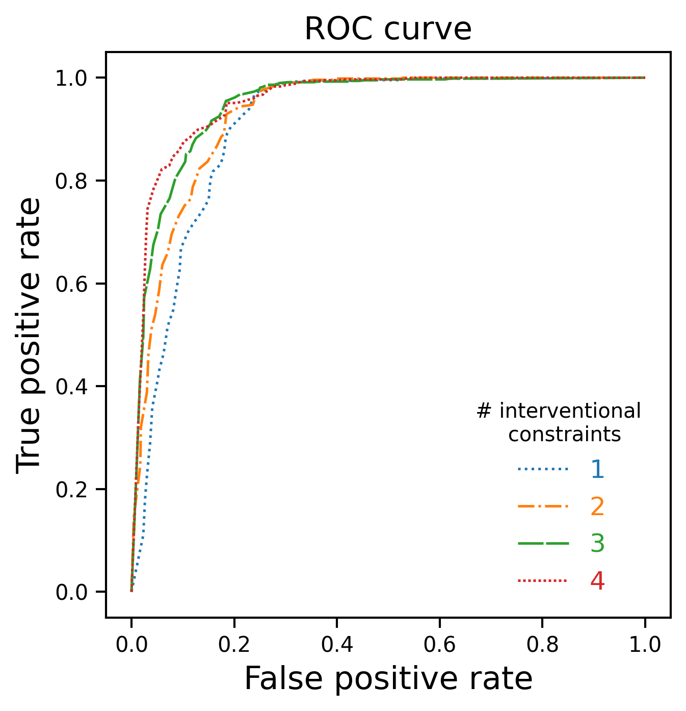
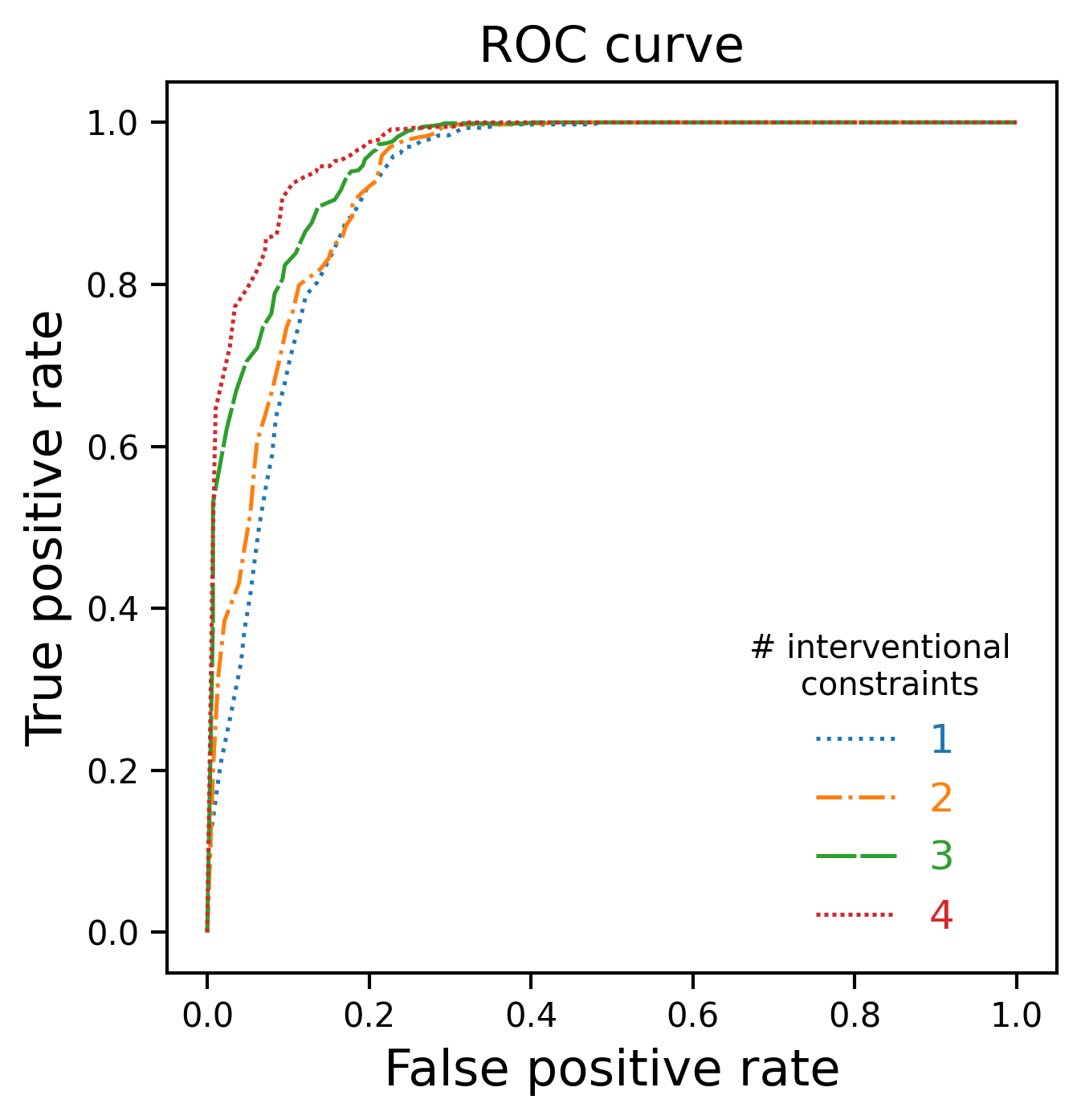
Setting 2: Evaluation of i/̄CMAXENT with combinations of interventional and conditional information. In this setting, we evaluate the performance of i/̄CMAXENT for causal feature selection when for a fraction of the variables interventional information is available, while for the other variables we have conditional information. With this experiment, we want to emulate something that can often occur in real datasets; that is, that not all the variables are intervenable. In this scenario we assume that we are given data on the full joint observational distribution of the potential causes.
We use Proposition 5.2 to decide which potential parent can provide interventional instead of conditional data. For example, in Figure 1(c), from Proposition 5.2 it follows that we can use as a constraint regardless of the existence of the dashed edges because it is identifiable. However, is not identifiable if the edge between and exists. As a result, we can only use conditional expectations for .
In both settings, we use the relative difference estimator defined in Garrido Mejia et al. (2022) as the parameter for the ROC curves of CMAXENT and i/̄CMAXENT (for details see Appendix C). For the ROC curve of the KCI test, we vary the threshold on the p-value of the test.
6.2 Joint interventional distributions from single interventions
We are interested in finding multivariate interventional distributions when our available data comes from single-variable interventions. For this task, we use the DAG shown in Figure 1(a) and sample 200 random graph instantiations.
We perform five experiments to assess how changing the amount and the type of information that we provide as constraints influences the estimation of the joint interventional probability . In all of these cases we use 1000 observations to compute the empirical averages: (1) We randomly chose two potential causes and , and we provide i/̄CMAXENT with constraints on . Additionally, we provide constraints on single-variable interventional distributions for the rest of the potential causes, that is, for all . (2) We only provide constraints on . (3) We only provide constraints on the single-variable interventional distributions for all potential causes for all . (4) We only provide constraints on the single-variable conditional distributions for all potential cause for all . This scenario coincides with CMAXENT. (5) As a baseline, we finally estimate MAXENT without constraints.
We then estimate the joint interventional distribution for each graph and plot the residuals from the true interventional distribution, as shown in Figure 2.
7 Results
7.1 Causal feature selection
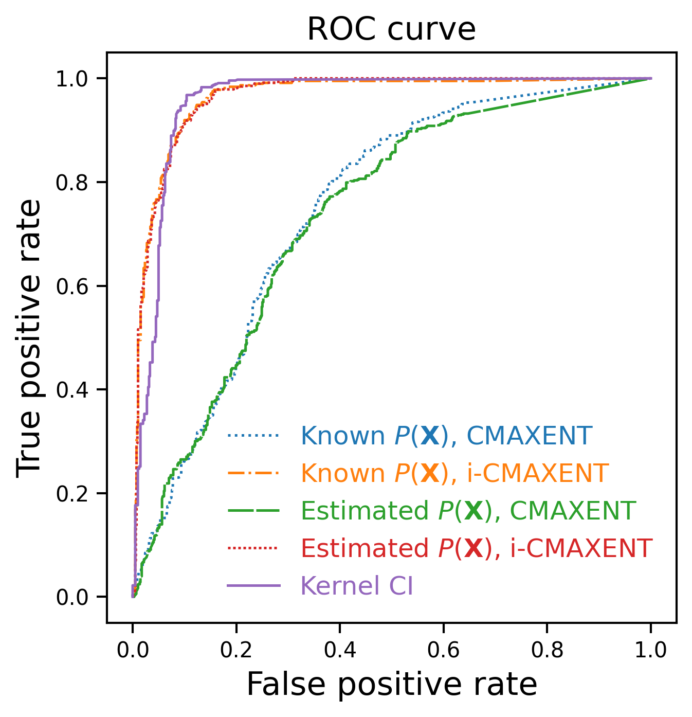

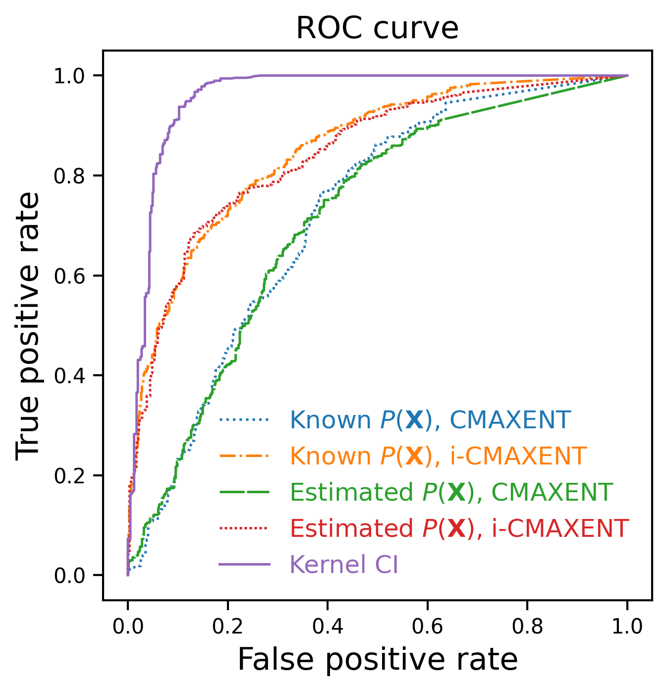
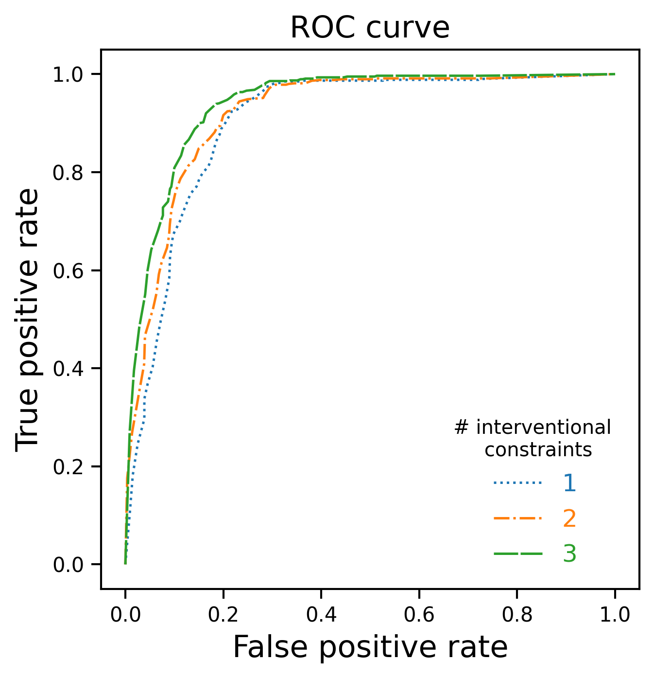
The three used types of graphs are shown in Figures 1(a), 1(b) and 1(c). In Figures 1(d), 1(e) and 1(f), we show the ROC curves for the detection of true causal arrows from to . The results show that i/̄CMAXENT outperforms CMAXENT in this task for all tested graph types. For graph types (a) and (b) we see that i/̄CMAXENT performs similarly well as KCI. But even for graph (c) where the potential causes interact with each other, we observe that the difference between i/̄CMAXENT and KCI is not too large.
Figures 1(g), 1(h) and 1(i) show the performance of i/̄CMAXENT in scenarios where information about the interventional distributions is provided as constraints only for a fraction of the potential causes, while for the remaining only conditional distributions are used. We observe that the causal features are recovered better as we increase the share of variables for which interventional data is provided.
7.2 Joint interventional distributions from single interventions
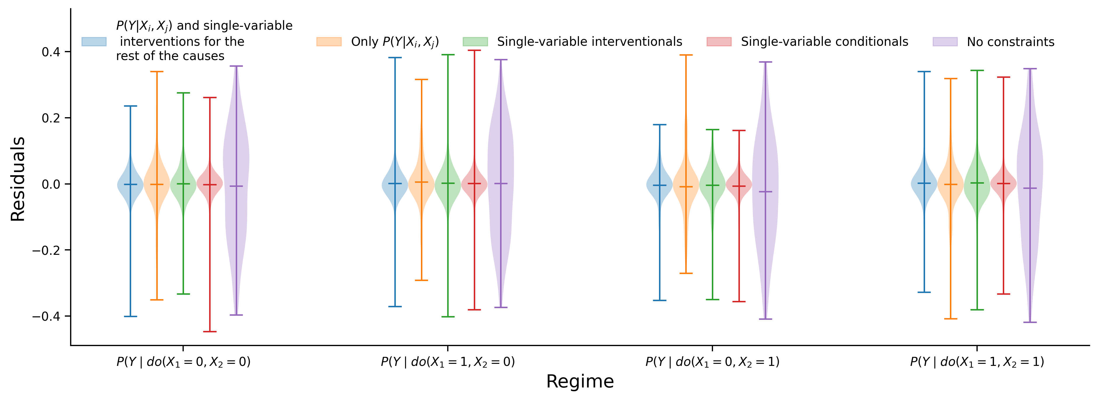
Figure 2 depicts the residuals between the estimated joint interventional distributions and the true joint interventional distributions for each combination of values that and can take. We observe that including any information as constraints to MAXENT improves the estimation of the interventional distributions, as expected. Furthermore, we observe that the error of the estimation using i/̄CMAXENT is on the order of , as long as we provide some type of constraint.
If we compare the residual distributions from different estimations, we can see that using only has higher variance than the rest of the scenarios, while using single-variable conditionals has (by a low margin) lower variance than the rest of them. Moreover, the extrema (the horizontal marks at of the end of each distribution) of the residuals have similar spread, depending on the regime.
8 Discussion
Causal marginal problem with interventional distributions. In Theorem 5.1 we prove, for the first time, that the causal marginal problem can be solved with interventional distributions as constraints using the Maximum Entropy principle, resulting in a solution that belongs to the exponential family. This implies that the solution to i/̄CMAXENT inherits the properties related to exponential families; that is, that assuming faithfulness f-expectations (Assumption 3), the Lagrange multipliers in the solution of i/̄CMAXENT can be used to read conditional independences in the graph Garrido Mejia et al. (2022). This extension allows us to leverage interventional information from RCTs that have been performed on subsets of variables, without requiring joint observations of all the variables. Thus, this method constitutes a foundational tool for many applications where the joint effect of disjoint treatments needs to be identified, given marginal information.
Causal feature selection using interventional data. Figure 1 depicted that i/̄CMAXENT performs very well in the task of causal feature selection in terms of ROCs even compared to methods that use the full joint distribution like KCI. In addition, it can combine information of different type (interventional, conditional) and to merge information from different sources (marginal structures) to perform causal feature selection in DAGs. This combination of data was not possible before in the state of the art merging literature (Garrido Mejia et al., 2022).
Joint interventional estimation. In Figure 2 we studied how the performance in estimating the joint interventional distribution changes when varying the type of information that is provided as constraints. As expected by the maximum entropy solution (Jaynes, 1957), providing no constraints of any type resulted in the uniform distribution. On the contrary, we see that the variance of the residuals from the true distribution becomes smaller when we increase the number of nodes for which we provide constraints. We observed that using only single-variable conditionals is, by a slight margin, a better set of constraints than single-variable interventional distributions.
This observation may raise some concern as it does not depict the same superiority of i/̄CMAXENT with interventional constraints over i/̄CMAXENT with conditional constraints ( CMAXENT) that was shown in the causal feature selection task (Figure 1). Nevertheless, one should be cautious in such conclusions, as the two tasks are not immediately comparable. While i/̄CMAXENT for CFS uses only the Lagrange multipliers to decide for a causal parent, the estimation task relies on the exact form of the inferred conditional distribution to further estimate the interventional joint.
Limitations. One of the limitations of our method is that we need to know which variables are intervened in each interventional expectation that is used as constraint in order to match the expectations that are given in the optimisation problem. This limitation is unavoidable, as Maximum Entropy estimations identify the exponential family distribution that have expectations close to those given as constraints. Existing methods for causal feature selection such as ICP (Peters et al., 2016; Heinze-Deml et al., 2018) do not need to know where the interventions were applied, only that they were applied on the potential causes and not on the target. Of course these methods can only operate when the joint observational distribution is known. Our method requires precise knowledge about the intervention but in return it allows causal feature selection under the more challenging causal marginal problem.
Relaxing the graph constraints for causal feature selection. In order to use i/̄CMAXENT for causal feature selection in environments with marginal experimentation, we have to make some assumptions on the causal graph (see Section 6), namely, that none of the potential causes is a child of the target node, and, that there are no hidden confounders between the potential causes and the target. While the latter constraint still remains, the former can be relaxed if at least one single-interventional distribution for each node of the potential causes is provided. Then we no longer require that the potential causes cannot be descendants of the target node, as we can screen off any children from being causes of the target.
Acknowledgements
This work was partly supported by the Amazon Hub project PSMEWE A03B “Merging data sources”.
References
- Berger et al. (1996) Berger, A., Della Pietra, S. A., and Della Pietra, V. J. A maximum entropy approach to natural language processing. Computational linguistics, 22(1):39–71, 1996.
- Bradbury et al. (2018) Bradbury, J., Frostig, R., Hawkins, P., Johnson, M. J., Leary, C., Maclaurin, D., Necula, G., Paszke, A., VanderPlas, J., Wanderman-Milne, S., and Zhang, Q. JAX: composable transformations of Python+NumPy programs, 2018. URL http://github.com/google/jax.
- Cooper & Yoo (1999) Cooper, G. F. and Yoo, C. Causal discovery from a mixture of experimental and observational data. In Proceedings of the Fifteenth conference on Uncertainty in artificial intelligence, pp. 116–125, 1999.
- Danks et al. (2008) Danks, D., Glymour, C., and Tillman, R. Integrating locally learned causal structures with overlapping variables. Advances in Neural Information Processing Systems, 21, 2008.
- Deming & Stephan (1940) Deming, W. E. and Stephan, F. F. On a least squares adjustment of a sampled frequency table when the expected marginal totals are known. The Annals of Mathematical Statistics, 11(4):427–444, 1940.
- Eaton & Murphy (2007) Eaton, D. and Murphy, K. Exact bayesian structure learning from uncertain interventions. In Meila, M. and Shen, X. (eds.), Proceedings of the Eleventh International Conference on Artificial Intelligence and Statistics, volume 2 of Proceedings of Machine Learning Research, pp. 107–114, San Juan, Puerto Rico, 21–24 Mar 2007. PMLR. URL https://proceedings.mlr.press/v2/eaton07a.html.
- Elahi et al. (2024) Elahi, M. Q., Ghasemi, M., and Kocaoglu, M. Identification of average causal effects in confounded additive noise models. arXiv preprint arXiv:2407.10014, 2024.
- Farnia & Tse (2016) Farnia, F. and Tse, D. A minimax approach to supervised learning. Advances in Neural Information Processing Systems, 29, 2016.
- Garrido Mejia et al. (2022) Garrido Mejia, S., Kirschbaum, E., and Janzing, D. Obtaining causal information by merging datasets with maxent. In International Conference on Artificial Intelligence and Statistics, pp. 581–603. PMLR, 2022.
- Gresele et al. (2022) Gresele, L., Von Kügelgen, J., Kübler, J., Kirschbaum, E., Schölkopf, B., and Janzing, D. Causal inference through the structural causal marginal problem. In International Conference on Machine Learning, pp. 7793–7824. PMLR, 2022.
- Heinze-Deml et al. (2018) Heinze-Deml, C., Peters, J., and Meinshausen, N. Invariant causal prediction for nonlinear models. Journal of Causal Inference, 6(2), 2018.
- Hindersah et al. (2022) Hindersah, R., Kalay, A. M., and Talahaturuson, A. Rice yield grown in different fertilizer combination and planting methods: Case study in buru island, indonesia. Open Agriculture, 7(1):871–881, 2022.
- Janzing (2021) Janzing, D. Causal versions of maximum entropy and principle of insufficient reason. Journal of Causal Inference, 9(1):285–301, 2021.
- Janzing et al. (2009) Janzing, D., Sun, X., and Schölkopf, B. Distinguishing cause and effect via second order exponential models. arXiv preprint arXiv:0910.5561, 2009.
- Jaynes (1957) Jaynes, E. T. Information theory and statistical mechanics. Physical review, 106(4):620, 1957.
- Jaynes (2003) Jaynes, E. T. Probability theory: The logic of science. Cambridge university press, 2003.
- Jeunen et al. (2022) Jeunen, O., Gilligan-Lee, C., Mehrotra, R., and Lalmas, M. Disentangling causal effects from sets of interventions in the presence of unobserved confounders. Advances in Neural Information Processing Systems, 35:27850–27861, 2022.
- Kellerer (1964) Kellerer, H. G. Maßtheoretische marginalprobleme. Mathematische Annalen, 153(3):168–198, June 1964. doi: 10.1007/bf01360315. URL https://doi.org/10.1007/bf01360315.
- Koller & Friedman (2009) Koller, D. and Friedman, N. Probabilistic graphical models: principles and techniques. MIT press, 2009.
- Mooij et al. (2020) Mooij, J. M., Magliacane, S., and Claassen, T. Joint causal inference from multiple contexts. The Journal of Machine Learning Research, 21(1):3919–4026, 2020.
- Pearl (2009) Pearl, J. Causality. Cambridge university press, 2009.
- Pearl & Mackenzie (2018) Pearl, J. and Mackenzie, D. The Book of Why: The New Science of Cause and Effect. Basic Books, Inc., USA, 1st edition, 2018. ISBN 046509760X.
- Peters et al. (2016) Peters, J., Bühlmann, P., and Meinshausen, N. Causal inference by using invariant prediction: identification and confidence intervals. Journal of the Royal Statistical Society: Series B (Statistical Methodology), 78(5):947–1012, 2016.
- Qiu et al. (2022) Qiu, H., Yang, S., Jiang, Z., Xu, Y., and Jiao, X. Effect of irrigation and fertilizer management on rice yield and nitrogen loss: A meta-analysis. Plants, 11(13):1690, 2022.
- Saengkyongam & Silva (2020) Saengkyongam, S. and Silva, R. Learning joint nonlinear effects from single-variable interventions in the presence of hidden confounders. In Conference on Uncertainty in Artificial Intelligence, pp. 300–309. PMLR, 2020.
- Sani et al. (2023) Sani, N., Mastakouri, A. A., and Janzing, D. Bounding probabilities of causation through the causal marginal problem. arXiv preprint arXiv:2304.02023, 2023.
- Sun et al. (2006) Sun, X., Janzing, D., and Schölkopf, B. Causal inference by choosing graphs with most plausible markov kernels. In Ninth International Symposium on Artificial Intelligence and Mathematics (AIMath 2006), pp. 1–11, 2006.
- Tian & Pearl (2001) Tian, J. and Pearl, J. Causal discovery from changes. In Proceedings of the Seventeenth conference on Uncertainty in artificial intelligence, pp. 512–521, 2001.
- Tian & Pearl (2002) Tian, J. and Pearl, J. A general identification condition for causal effects. eScholarship, University of California, 2002.
- Tillman & Spirtes (2011) Tillman, R. and Spirtes, P. Learning equivalence classes of acyclic models with latent and selection variables from multiple datasets with overlapping variables. In Proceedings of the Fourteenth International Conference on Artificial Intelligence and Statistics, pp. 3–15. JMLR Workshop and Conference Proceedings, 2011.
- Tillman (2009) Tillman, R. E. Structure learning with independent non-identically distributed data. In Proceedings of the 26th Annual International Conference on Machine Learning, pp. 1041–1048, 2009.
- Triantafillou & Tsamardinos (2015) Triantafillou, S. and Tsamardinos, I. Constraint-based causal discovery from multiple interventions over overlapping variable sets. The Journal of Machine Learning Research, 16(1):2147–2205, 2015.
- Wainwright et al. (2008) Wainwright, M. J., Jordan, M. I., et al. Graphical models, exponential families, and variational inference. Foundations and Trends® in Machine Learning, 1(1–2):1–305, 2008.
- Wihardjaka et al. (2022) Wihardjaka, A., Harsanti, E. S., and Ardiwinata, A. N. Effect of fertilizer management on potassium dynamics and yield of rainfed lowland rice in indonesia. Chilean journal of agricultural research, 82(1):33–43, 2022.
- Zhang et al. (2011) Zhang, K., Peters, J., Janzing, D., and Schölkopf, B. Kernel-based conditional independence test and application in causal discovery. In 27th Conference on Uncertainty in Artificial Intelligence (UAI 2011), pp. 804–813. AUAI Press, 2011.
Appendix A Proofs of the main results
See 5.1
Proof.
We start by setting up the Lagrangian, where we have one for each constraint in our optimisation problem.
| (7) | ||||
| (8) | ||||
| (9) | ||||
| (10) | ||||
| (11) |
In the following, we will use and to denote elements of the set and . We will denote the complement of in as . So, in that order of ideas, .
In other words, 444Of course can be the composition of sums, just as . Differentiating with respect to each and all the multipliers, we obtain
| (12) | ||||
Notice that the derivative with respect to the Lagrangian in Equation 12 is 0 for those functions and for which .
We then find the solution to when the above equations are equal to 0. From Equation 12 we get
| (13) | ||||
| (14) |
It is important to notice that this equation is well-defined as long as for all . Because the elements inside the exponential depend on , we can rename with . In addition, we gather the constants into the normalizing constant, which depends on , giving us
| (15) |
as required. ∎
See 5.2
Proof.
Because of the assumed generative process, the causal sufficiency assumption, and the fact that is the only potential child of , there are no “bidirectional” arrows connected to any child of in the sense of Tian & Pearl (2002). As a result, the conditions of Theorem 2 in Tian & Pearl (2002) apply and is identifiable using observational quantities.
We have just proved the identifiability of the interventional distribution. Now we would like to prove that the set is a valid adjustment set. This is true for the following reasons. First, the assumption of the three levels of the generative process, which has as a consequence that there is no collider (or descendants of a collider) between and the elements in . Second, Assumption (1) which states there is no unobserved confounder between and , thus blocks any potential backdoor path between and through any confounder. ∎
Appendix B Computation of Maxent through norm minimisation
As shown in Theorem (1), the interventional maximum entropy solution is equivalent to maximum likelihood where the dual variables are the parameters of the exponential family. We will now show how the maximum likelihood problem can be expressed as the minimisation between the difference between the given empirical averages and the expectations of the functions given the exponential family distribution. The way we maximise Equation 15 for all our data, with respect to the Lagrange multipliers (the ), is by making equal to 0 the derivative of the log-likelihood with respect to the parameters:
| (16) |
Because we have empirical averages, the previous equation (for the whole data) becomes
| (17) |
which we can compute by using any method that minimises the difference between the observed empirical average and the entailed expectation using the exponential family distribution. That is, we can compute the solution to the dual problem of the exponential family with
| (18) |
The result in Equation 17 is not new (see, for example Wainwright et al. (2008, Sec. 3.1)). However, the use of this fact to compute the resulting exponential family even in scenarios with missing data is new to us.
In the synthetic experiments Section (6), there were situations where . We fixed this by adding a machine epsilon to all possible combinations and renormalizing.
Appendix C Relative difference estimator
The relative difference estimator introduced in (Garrido Mejia et al., 2022) is an estimator of how close two parameters are to each other so that an analyst can decide whether there exist conditional independence. The relative difference estimator can take values between 0 and 1. However, there is no probabilistic analysis of the estimator, so one cannot consider the value of the relative difference estimator as a well-calibrated probability of the difference between multipliers (or difference between a multiplier and 0). The estimator is defined as
| (19) |
where are the two Lagrange multipliers for the constraints associated with .
Appendix D Optimisation and convergence
To find the Lagrange multipliers, using the norm minimisation procedure explained in Appendix B, we use the Broyden–Fletcher–Goldfarb–Shanno (BFGS) algorithm implemented in the JAX Python library (Bradbury et al., 2018). We consider an estimation as converged if the norm (the sum of the squared of the residuals between the empirical averages given as constraints and the expectations entailed by the exponential family distribution) are less than , or if the optimiser terminates successfully. In some cases, convergence in this sense is not achieved on the first application of the optimisation algorithm. When this happens, we simply use the optimisation algorithm again using the previously found Lagrange multipliers as the initial values for the optimisation. We repeat this process until convergence in the above sense is achieved. We found that in most cases one extra optimisation is enough to achieve convergence, there were four cases where we had to run the optimiser more than two times: twice for three, once for four, and once for five.