The breaking of $f-$mode universal relation in proto-neutron stars

Abstract

Proto-neutron stars have both high-density and relatively high-temperature in them. This study analyses how the equation of state changes with temperature, which is relevant for proto-neutron stars. We determine an equation of state for the proto-neutron stars in the relativistic mean field model in which the coupling parameters are density-dependent. The equation of state considerably affects the mass-radius curve, thereby affecting the f-mode oscillation frequency. Temperature makes the equation of state stiffer at relatively low and intermediate densities, thereby making the star less compact and the mass-radius curve flatter. The f-mode frequency for low and intermediate-mass neutron stars decreases with temperature and thus should be easier to detect. The universal relation (connecting f-mode frequency, mass and radius) changes non-linearly with temperature. The parameters defining the universal relation ($\omega M=a(T)\left(\frac{M}{R}\right)+b(T)$) becomes temperature dependent with the coefficients following a parabolic relation with temperature.

I Introduction

nss are the densest objects in the universe after the bhs that emerge as remnants of supernovae explosions. As natural astrophysical laboratories, these stellar remnants provide valuable insights into the fundamental physics, astrophysics, and the behaviour of matter under extreme densities, pressures and temperatures. The density in the core can reach up to a few times nuclear saturation density ($\rho_{0}=1.6\ {\rm fm}^{-3}$) and temperature can reach up to a few tens of MeV ($1\ {\rm MeV}\sim 10^{10}\ {\rm K}$) at the birth of ns. The matter under such extreme conditions is interesting to study, giving insights into the properties of strong interactions at a fundamental level [1]. At such extreme conditions, one can expect different phases of normal nuclear matter such as hqpt [2, 3], loff [4, 5], cfl [6, 7, 8, 9, 10], csc [11, 12, 13] or other exotic matter phases[14, 15, 16] along with usual nuclear matter.

NS emerges from the supernova explosion, where the inner core of a massive star (more than 20 $M_{\odot}$) undergoes a rapid collapse because of unbalancing gravitational force, leading to an increase in temperature and density. The gravitational energy released during the collapse results in shock waves that propel the star’s outer layers into space and leave behind a compact, extremely hot core, which we call a pns. At this point, the electron neutrino attains a finite chemical potential for a while (up to 10-20 s) due to the small mean free path. After that, electron neutrinos escape the core, and again, the matter attains hydrostatic equilibrium, i.e. inverted gravitational force is balanced with the outward degenerate gas pressure. The temperature of the nascent ns can reach upto 60 MeV [17, 18, 19]. After the birth, it starts to cool. In a few hundred years, it cools down to the temperature of a few hundred eV [20, 21].

Right after their birth, nss known as proto-neutron stars (PNSs) are unstable and oscillate considerably. They can have both radial and non-radial oscillations, and the frequency of their oscillations depends on their physical and thermodynamic properties. The study of stellar oscillations, known as asteroseismology [22], is a very useful technique to understand the inner structure and composition of such compact objects [3, 23]. In recent studies, the radial and non-radial oscillations of nss have become very important because they are very sensitive to the matter present in the interior of nss [24]. Different studies have found various universal/quasi-universal relations (simple linear relationships) between the non-radial oscillation frequencies, masses, and radii of the cold nss [3]. This intrigues whether these relations would hold even for the hot nss or if they deviate from them.

One simple way to indirectly detect non-radial oscillation modes is through GWs. The non-radial oscillations of nss dump their energy into the gws signal during the inspiral of the binary [25]. The oscillating nss emit gw with different modes of frequencies, such as $g$, $f$, and $p$, etc., depending on the nature of the restoring forces. Therefore, the oscillation frequencies depend strongly on the internal compositions and the various properties of nss. Among them, $g$-modes have the lowest frequencies and are more likely to be detected with 3rd generation detectors or even with present detectors. However, they usually appear when there is a strong temperature or composition gradient in the NS. The p-mode frequencies are usually relatively high and are not expected to be detected with present detectors. Therefore, in this study, we focus our attention on the f-mode frequency, which lies in the 1-3 kHz band. The main aim of the study is to analyze how NS properties, along with the f-mode frequency and the universal relation, behave when we have a finite temperature effect in the matter, which is usually the case with proto-neutron stars. This will help us in understanding and constraining the matter inside hot NSs and proto-neutron stars [26, 3, 27]

In the present analysis, we study the asteroseismology of pns. We present the non-radial oscillations, especially the $f$-modes at different stages of ns as it cools down and gives the temperature-dependent urs relating the masses, radii and the $f$-mode oscillation frequencies of nss. The precision in the measurements of macroscopic properties of ns, such as mass, radius, tidal deformability etc, contribute to our understanding of eos of nuclear matter under extreme conditions. It is difficult to determine the true nature of matter due to the significant uncertainties in observations such as radius in electromagnetic spectrum [28, 29, 30, 31]. Asteroseismology can be another tool to probe matter properties in isolated ns. While some of the aspects have been explored in the previous studies [32, 33, 34, 35, 36, 37] the present investigation gives some new insights on the finite temperature aspects of nss. It may be mentioned here that the non-radial $g$-mode oscillations at finite temperatures have been studied using a meta-model in Ref. [38]; on the other hand, we shall study here the non-radial thermal $f$-mode oscillations within the ambit of rmf models for nuclear matter at finite temperature.

We start with the description of eos at various temperatures in the rmf model with the density-dependent coupling parameters [39]. Then, we show the validity of the urs at various temperatures. The structure of the article is as follows. In section II, we discuss the EOS of NS matter in relativistic mean field theory. We give brief formalism of non-radial oscillation in section III. In section IV, we discuss the results of the present work and summarize it in section V. Throughout the article, we assume $G=1=c=\hbar$.

II Nuclear matter equation of state

In this section, we briefly discuss eos of nuclear matter relevant for pnss. We consider rmf model description of nuclear matter present in the core of pnss. The Lagrangian of our model is as follows [40, 3, 41]

$$\halign to=0.0pt{\relax\global\advance\@IEEEeqncolcnt by 1\relax\begingroup\csname @IEEEeqnarraycolPREr\endcsname#\relax\relax\relax\relax\relax\relax\relax\relax\relax\relax\csname @IEEEeqnarraycolPOSTr\endcsname\relax\relax\relax\relax\relax\relax\relax\relax\relax\relax\endgroup&\relax\global\advance\@IEEEeqncolcnt by 1\relax\begingroup\csname @IEEEeqnarraycolPREC\endcsname#\relax\relax\relax\relax\relax\relax\relax\relax\relax\relax\csname @IEEEeqnarraycolPOSTC\endcsname\relax\relax\relax\relax\relax\relax\relax\relax\relax\relax\endgroup&\relax\global\advance\@IEEEeqncolcnt by 1\relax\begingroup\csname @IEEEeqnarraycolPREl\endcsname#\relax\relax\relax\relax\relax\relax\relax\relax\relax\relax\csname @IEEEeqnarraycolPOSTl\endcsname\relax\relax\relax\relax\relax\relax\relax\relax\relax\relax\endgroup&\global\advance\@IEEEeqncolcnt by 1\relax\bgroup#\egroup&\global\advance\@IEEEeqncolcnt by 1\relax\hbox to\z@\bgroup\hss#\egroup\cr\hfil$\displaystyle\mathcal{L} $&\hfil$\displaystyle{}={}$\hfil&$\displaystyle\sum_{b} \left[\bar{\psi}_{b} \bigg{(}i \gamma_{\mu}\partial^{\mu} - m_{b} +g_{\sigma b}\sigma-g_{\omega b}\gamma_{\mu}\omega^{\mu}\right. \left. - \frac{1}{2}g_{\rho b} {\bm{\rho}}_{\mu}\cdot{\bm{\tau}} \gamma^{\mu}\bigg{)}\psi_{b}\right] $\hfil&{{}\vrule width=0.0pt,height=0.0pt,depth=0.0pt&0.0pt{\hss(1)}\cr\penalty 100\vskip 3.0pt\vskip 0.0pt\cr}&+\frac{1}{2}\left[\partial_{\mu}\sigma\partial^{\mu}\sigma-m_{\sigma}^{2}\sigma^{2}\right]+\frac{1}{2}\left[-\frac{1}{2}\Omega_{\mu\nu}\Omega^{\mu\nu}+m_{\omega}^{2}\omega_{\mu}\omega^{\mu}\right]+\frac{1}{2}\left[-\frac{1}{2}R_{\mu\nu}R^{\mu\nu}-m_{\rho}^{2}{\bm{\rho}}_{\mu}{\bm{\rho}}^{\mu}\right]\vrule width=0.0pt,height=0.0pt,depth=0.0pt(2)\cr}$$

where $\psi_{b}$ represent the baryon with bare mass $m_{b}$. The interactions between the baryons are governed by the exchange of mesons ($\sigma$ and $\omega$). The scalar meson ($\sigma$) exchange provides attraction interaction, while the vector meson exchange ($\omega$) provides repulsive interaction. We also include an isovector meson ($\rho$) to have isospin asymmetry between baryons. The symbols $\Omega_{\mu\nu}$, and ${\bm{R}}_{\mu\nu}$ represent the field strength tensors corresponding to the vector and iso-vector fields $\omega_{\mu}$, and ${\bm{\rho}}_{\mu}$ respectively. The first and the last terms correspond to the Dirac Lagrangian for baryons and leptons, respectively. The rest of the terms correspond to mesons, where we have taken a Klein Gordan Lagrangian density for the scalar $\sigma$ field and a Proca Lagrangian density for the massive vector fields $\omega_{\mu}$, and ${\bm{\rho}}_{\mu}$ fields. The operators ${\bm{\tau}}$ are the Pauli isospin matrices. The meson couplings are to be considered as density-dependent as [42, 43]

$$\halign to=0.0pt{\relax\global\advance\@IEEEeqncolcnt by 1\relax\begingroup\csname @IEEEeqnarraycolPREr\endcsname#\relax\relax\relax\relax\relax\relax\relax\relax\relax\relax\csname @IEEEeqnarraycolPOSTr\endcsname\relax\relax\relax\relax\relax\relax\relax\relax\relax\relax\endgroup&\relax\global\advance\@IEEEeqncolcnt by 1\relax\begingroup\csname @IEEEeqnarraycolPREC\endcsname#\relax\relax\relax\relax\relax\relax\relax\relax\relax\relax\csname @IEEEeqnarraycolPOSTC\endcsname\relax\relax\relax\relax\relax\relax\relax\relax\relax\relax\endgroup&\relax\global\advance\@IEEEeqncolcnt by 1\relax\begingroup\csname @IEEEeqnarraycolPREl\endcsname#\relax\relax\relax\relax\relax\relax\relax\relax\relax\relax\csname @IEEEeqnarraycolPOSTl\endcsname\relax\relax\relax\relax\relax\relax\relax\relax\relax\relax\endgroup&\global\advance\@IEEEeqncolcnt by 1\relax\bgroup#\egroup&\global\advance\@IEEEeqncolcnt by 1\relax\hbox to\z@\bgroup\hss#\egroup\cr\hfil$\displaystyle g_{\sigma i} $&\hfil$\displaystyle{}={}$\hfil&$\displaystyle g_{\sigma 0}\exp(-(x^{a_{\sigma}}-1)), $\hfil&{{}\vrule width=0.0pt,height=0.0pt,depth=0.0pt}&0.0pt{\hss(3)}\cr\penalty 100\vskip 3.0pt\vskip 0.0pt\cr\hfil$\displaystyle g_{\omega i} $&\hfil$\displaystyle{}={}$\hfil&$\displaystyle g_{\omega 0}\exp(-(x^{a_{\omega}}-1)), $\hfil&{{}\vrule width=0.0pt,height=0.0pt,depth=0.0pt}&0.0pt{\hss(4)}\cr\penalty 100\vskip 3.0pt\vskip 0.0pt\cr\hfil$\displaystyle g_{\rho i} $&\hfil$\displaystyle{}={}$\hfil&$\displaystyle g_{\rho 0}\exp(-a_{\rho}(x-1)), $\hfil&{\vrule width=0.0pt,height=0.0pt,depth=0.0pt}&0.0pt{\hss(5)}\cr}$$

where $x=\rho/\rho_{0}$ and $g_{\sigma 0}$, $g_{\omega 0}$, $g_{\rho 0}$, $a_{\sigma}$, $a_{\omega}$ and, $a_{\rho}$ are the model parameters, and given in the table 1.

From a given Lagrangian, Eq (II), we find eos with mean field approximation. In mean field approximation, we take the meson fields to be classical mean fields and retain the quantum nature of baryonic field i.e. $\langle\sigma\rangle=\sigma_{0}$, $\langle\omega_{\mu}\rangle=\omega_{0}\delta_{\mu 0}$, $\langle\rho_{\mu}^{a}\rangle$ = $\delta_{\mu 0}\delta_{a3}\rho_{03}$. In this approximation, we can define the effective masses and effective chemical potentials for baryons as

$$\halign to=0.0pt{\relax\global\advance\@IEEEeqncolcnt by 1\relax\begingroup\csname @IEEEeqnarraycolPREr\endcsname#\relax\relax\relax\relax\relax\relax\relax\relax\relax\relax\csname @IEEEeqnarraycolPOSTr\endcsname\relax\relax\relax\relax\relax\relax\relax\relax\relax\relax\endgroup&\relax\global\advance\@IEEEeqncolcnt by 1\relax\begingroup\csname @IEEEeqnarraycolPREC\endcsname#\relax\relax\relax\relax\relax\relax\relax\relax\relax\relax\csname @IEEEeqnarraycolPOSTC\endcsname\relax\relax\relax\relax\relax\relax\relax\relax\relax\relax\endgroup&\relax\global\advance\@IEEEeqncolcnt by 1\relax\begingroup\csname @IEEEeqnarraycolPREl\endcsname#\relax\relax\relax\relax\relax\relax\relax\relax\relax\relax\csname @IEEEeqnarraycolPOSTl\endcsname\relax\relax\relax\relax\relax\relax\relax\relax\relax\relax\endgroup&\global\advance\@IEEEeqncolcnt by 1\relax\bgroup#\egroup&\global\advance\@IEEEeqncolcnt by 1\relax\hbox to\z@\bgroup\hss#\egroup\cr\hfil$\displaystyle M_{i} $&\hfil$\displaystyle{}={}$\hfil&$\displaystyle m_{i} - g_{\sigma i} \sigma_{0} $\hfil&{{}\vrule width=0.0pt,height=0.0pt,depth=0.0pt}&0.0pt{\hss(6)}\cr\penalty 100\vskip 3.0pt\vskip 0.0pt\cr\hfil$\displaystyle\tilde{\mu}_{i} $&\hfil$\displaystyle{}={}$\hfil&$\displaystyle\mu_{i}-g_{\omega i}\omega_{0}-g_{\rho i}I_{3i}\rho_{03}-g_{\phi i}\phi_{0}-\Sigma^{r}. $\hfil&{\vrule width=0.0pt,height=0.0pt,depth=0.0pt}&0.0pt{\hss(7)}\cr}$$

where the term $\Sigma^{r}$ appears in Eq (II) because of the density-dependent meson couplings [3, 39, 44]. Historically, it is called the ‘rearrangement’ term [43]. By using the Lagrange-Euler equations or minimizing the thermal potential corresponding to the Lagrangian, Eq (II) with respect to the mean fields, we can find the meson field equations as follows

$$\halign to=0.0pt{\relax\global\advance\@IEEEeqncolcnt by 1\relax\begingroup\csname @IEEEeqnarraycolPREr\endcsname#\relax\relax\relax\relax\relax\relax\relax\relax\relax\relax\csname @IEEEeqnarraycolPOSTr\endcsname\relax\relax\relax\relax\relax\relax\relax\relax\relax\relax\endgroup&\relax\global\advance\@IEEEeqncolcnt by 1\relax\begingroup\csname @IEEEeqnarraycolPREC\endcsname#\relax\relax\relax\relax\relax\relax\relax\relax\relax\relax\csname @IEEEeqnarraycolPOSTC\endcsname\relax\relax\relax\relax\relax\relax\relax\relax\relax\relax\endgroup&\relax\global\advance\@IEEEeqncolcnt by 1\relax\begingroup\csname @IEEEeqnarraycolPREl\endcsname#\relax\relax\relax\relax\relax\relax\relax\relax\relax\relax\csname @IEEEeqnarraycolPOSTl\endcsname\relax\relax\relax\relax\relax\relax\relax\relax\relax\relax\endgroup&\global\advance\@IEEEeqncolcnt by 1\relax\bgroup#\egroup&\global\advance\@IEEEeqncolcnt by 1\relax\hbox to\z@\bgroup\hss#\egroup\cr\hfil$\displaystyle m_{\sigma}^{2} \sigma_{0} $&\hfil$\displaystyle{}={}$\hfil&$\displaystyle\sum_{i} g_{\sigma i} \rho_{s}^{i}, $\hfil&{{}\vrule width=0.0pt,height=0.0pt,depth=0.0pt}&0.0pt{\hss(8)}\cr\penalty 100\vskip 3.0pt\vskip 0.0pt\cr\hfil$\displaystyle m_{\omega}^{2} \omega_{0} $&\hfil$\displaystyle{}={}$\hfil&$\displaystyle\sum_{i} g_{\omega i} \rho^{i}, $\hfil&{{}\vrule width=0.0pt,height=0.0pt,depth=0.0pt}&0.0pt{\hss(9)}\cr\penalty 100\vskip 3.0pt\vskip 0.0pt\cr\hfil$\displaystyle m_{\rho}^{2} \rho_{0} $&\hfil$\displaystyle{}={}$\hfil&$\displaystyle\sum_{i} g_{\rho i} I_{3i} \rho^{i}. $\hfil&{\vrule width=0.0pt,height=0.0pt,depth=0.0pt}&0.0pt{\hss(10)}\cr}$$

In the above $\rho_{s}^{i}$ and $\rho^{i}$ is the scalar and vector density of the $i^{\rm th}$ baryon is defined as

$$\halign to=0.0pt{\relax\global\advance\@IEEEeqncolcnt by 1\relax\begingroup\csname @IEEEeqnarraycolPREr\endcsname#\relax\relax\relax\relax\relax\relax\relax\relax\relax\relax\csname @IEEEeqnarraycolPOSTr\endcsname\relax\relax\relax\relax\relax\relax\relax\relax\relax\relax\endgroup&\relax\global\advance\@IEEEeqncolcnt by 1\relax\begingroup\csname @IEEEeqnarraycolPREC\endcsname#\relax\relax\relax\relax\relax\relax\relax\relax\relax\relax\csname @IEEEeqnarraycolPOSTC\endcsname\relax\relax\relax\relax\relax\relax\relax\relax\relax\relax\endgroup&\relax\global\advance\@IEEEeqncolcnt by 1\relax\begingroup\csname @IEEEeqnarraycolPREl\endcsname#\relax\relax\relax\relax\relax\relax\relax\relax\relax\relax\csname @IEEEeqnarraycolPOSTl\endcsname\relax\relax\relax\relax\relax\relax\relax\relax\relax\relax\endgroup&\global\advance\@IEEEeqncolcnt by 1\relax\bgroup#\egroup&\global\advance\@IEEEeqncolcnt by 1\relax\hbox to\z@\bgroup\hss#\egroup\cr\hfil$\displaystyle\rho_{s}^{i} $&\hfil$\displaystyle{}={}$\hfil&$\displaystyle-\gamma\int\frac{d{\bm{p}}}{(2\pi)^{3}} \frac{m_{i}^{\star}}{\sqrt{{\bm{p}}^{2} + {M_{i}}^{2}}} \left(1 - f_{-}^{i} - f_{+}^{i} \right) $\hfil&{{}\vrule width=0.0pt,height=0.0pt,depth=0.0pt}&0.0pt{\hss(11)}\cr\penalty 100\vskip 3.0pt\vskip 0.0pt\cr\hfil$\displaystyle\rho^{i} $&\hfil$\displaystyle{}={}$\hfil&$\displaystyle\gamma\int\frac{d{\bm{p}}}{(2\pi)^{3}} \left( f_{-}^{i} - f_{+}^{i} \right), $\hfil&{\vrule width=0.0pt,height=0.0pt,depth=0.0pt}&0.0pt{\hss(12)}\cr}$$

respectively, where $\gamma=2$ is the spin degeneracy factor. The Eqs. (II - II) are the coupled equations and need to be solved simultaneously. For the sake of completeness, we here present eos which is as follows

$$\halign to=0.0pt{\relax\global\advance\@IEEEeqncolcnt by 1\relax\begingroup\csname @IEEEeqnarraycolPREr\endcsname#\relax\relax\relax\relax\relax\relax\relax\relax\relax\relax\csname @IEEEeqnarraycolPOSTr\endcsname\relax\relax\relax\relax\relax\relax\relax\relax\relax\relax\endgroup&\relax\global\advance\@IEEEeqncolcnt by 1\relax\begingroup\csname @IEEEeqnarraycolPREC\endcsname#\relax\relax\relax\relax\relax\relax\relax\relax\relax\relax\csname @IEEEeqnarraycolPOSTC\endcsname\relax\relax\relax\relax\relax\relax\relax\relax\relax\relax\endgroup&\relax\global\advance\@IEEEeqncolcnt by 1\relax\begingroup\csname @IEEEeqnarraycolPREl\endcsname#\relax\relax\relax\relax\relax\relax\relax\relax\relax\relax\csname @IEEEeqnarraycolPOSTl\endcsname\relax\relax\relax\relax\relax\relax\relax\relax\relax\relax\endgroup&\global\advance\@IEEEeqncolcnt by 1\relax\bgroup#\egroup&\global\advance\@IEEEeqncolcnt by 1\relax\hbox to\z@\bgroup\hss#\egroup\cr\hfil$\displaystyle p = - \epsilon+ \frac{1}{\beta}s + \sum_{i} \mu_{i} \rho_{i}, $&\hfil$\displaystyle{}{}$\hfil&$\displaystyle$\hfil&{\vrule width=0.0pt,height=0.0pt,depth=0.0pt}&0.0pt{\hss(13)}\cr}$$

where $p$, $\epsilon$, $\beta$ and $s$ represent the total pressure, total energy density, inverse of temperature ($\beta=1/T$) and total entropy density of $i^{\rm th}$ baryon, respectively. All these quantities are defined as follows

$$\halign to=0.0pt{\relax\global\advance\@IEEEeqncolcnt by 1\relax\begingroup\csname @IEEEeqnarraycolPREr\endcsname#\relax\relax\relax\relax\relax\relax\relax\relax\relax\relax\csname @IEEEeqnarraycolPOSTr\endcsname\relax\relax\relax\relax\relax\relax\relax\relax\relax\relax\endgroup&\relax\global\advance\@IEEEeqncolcnt by 1\relax\begingroup\csname @IEEEeqnarraycolPREC\endcsname#\relax\relax\relax\relax\relax\relax\relax\relax\relax\relax\csname @IEEEeqnarraycolPOSTC\endcsname\relax\relax\relax\relax\relax\relax\relax\relax\relax\relax\endgroup&\relax\global\advance\@IEEEeqncolcnt by 1\relax\begingroup\csname @IEEEeqnarraycolPREl\endcsname#\relax\relax\relax\relax\relax\relax\relax\relax\relax\relax\csname @IEEEeqnarraycolPOSTl\endcsname\relax\relax\relax\relax\relax\relax\relax\relax\relax\relax\endgroup&\global\advance\@IEEEeqncolcnt by 1\relax\bgroup#\egroup&\global\advance\@IEEEeqncolcnt by 1\relax\hbox to\z@\bgroup\hss#\egroup\cr\hfil$\displaystyle\epsilon$&\hfil$\displaystyle{}={}$\hfil&$\displaystyle- \gamma\sum_{i} \int\frac{d^{3}{\bm{p}}}{(2\pi)^{3}} \sqrt{{M_{i}}^{2} + {\bm{p}}^{2}}\left( 1 - f^{i}_{-} - f^{i}_{+} \right) $\hfil&{{}\vrule width=0.0pt,height=0.0pt,depth=0.0pt}&0.0pt{\hss(14)}\cr\penalty 100\vskip 3.0pt\vskip 0.0pt\cr\hfil$\displaystyle$&\hfil$\displaystyle{}{}$\hfil&$\displaystyle+ \sum_{i}\left(g_{\omega i}\omega_{0}+g_{\phi i}\phi_{0}+g_{\rho i}\rho_{03}I_{3i}\right) \rho^{i} + \frac{1}{2}\left( m_{\sigma}^{2}\sigma_{0}^{2} + m_{\omega}^{2}\omega_{0}^{2} + m_{\phi}^{2}\phi_{0}^{2} + m_{\rho}^{2}\rho_{03}^{2} \right), $\hfil&{{}\vrule width=0.0pt,height=0.0pt,depth=0.0pt}&0.0pt{\hss(15)}\cr\penalty 100\vskip 3.0pt\vskip 0.0pt\cr\hfil$\displaystyle s $&\hfil$\displaystyle{}={}$\hfil&$\displaystyle- \gamma\sum_{i} \int\frac{d^{3}{\bm{p}}}{(2\pi)^{3}} \left[ f^{i}_{-} \ln f^{i}_{-} + (1 - f^{i}_{-}) \ln(1 - f^{i}_{-})\right. + \left. \left(- \to+ \right)\right], $\hfil&{\vrule width=0.0pt,height=0.0pt,depth=0.0pt}&0.0pt{\hss(16)}\cr}$$

where $f^{i}_{-}$ ($f^{i}_{+}$) is the Fermi distribution of $i_{\rm th}$ particle (anti-particle) and defined as

$$f^{i}_{\pm}=\frac{1}{1+\exp[\beta(\sqrt{{M_{i}}^{2}+{\bm{p}}^{2}}\mp\tilde{\mu}_{i})]}.$$

Where $M_{i}$ and $\tilde{\mu}_{i}$ are defined in Eqs (II and II).

Table 1: The rmf model parameters [45, 46, 43, 3] and corresponding nuclear saturation properties of nuclear matter at saturation density $\rho_{0}=0.15\ {\rm fm}^{-3}$ and binding energy per baryon comes $\epsilon_{0}=-16.10\ {\rm MeV}$, where $N$ in coupling constants stands for neutron and proton only.

Coupling	Numerical	Nuclear	Numerical
parameters	values	saturation	values
		quantities	(MeV)
$g_{\sigma N0}$	9.180364	$K_{0}$	231
$g_{\omega N0}$	10.981329	$Q_{0}$	-109
$g_{\rho N0}$	3.826364	$Z_{0}$	1621
$a_{\sigma}$	0.086372	$J_{\rm sym,0}$	32.19
$a_{\omega}$	0.054065	$L_{\rm sym,0}$	41.26
$a_{\rho}$	0.509147	$K_{\rm sym,0}$	-116
$\cdots$	$\cdots$	$Q_{\rm sym,0}$	966
$\cdots$	$\cdots$	$Z_{\rm sym,0}$	-6014

Table 2: List of eoss, which we take to study the urs for pns. These eoss are taken from the CompOSE data library.

EOS	Refs.	EOS	Refs.
BHB$\Lambda\Phi$	[47, 48, 49, 50]	GRDF1 (DD2)	[51, 52, 39, 53]
HSB	[50, 54, 55]	HSB SF	[50, 56, 57]
STOS (TM1)	[58, 56]	VE (RNF)	[59, 60]
SHO (FSU2)	[50, 39, 57]	$\cdots$	$\cdots$

III Non-radial fluid oscillations of neutron stars

This section outlines the equations governing the oscillations of ns fluid comprising ns matter. We start with the most general metric for a spherically symmetric space-time

$$\halign to=0.0pt{\relax\global\advance\@IEEEeqncolcnt by 1\relax\begingroup\csname @IEEEeqnarraycolPREr\endcsname#\relax\relax\relax\relax\relax\relax\relax\relax\relax\relax\csname @IEEEeqnarraycolPOSTr\endcsname\relax\relax\relax\relax\relax\relax\relax\relax\relax\relax\endgroup&\relax\global\advance\@IEEEeqncolcnt by 1\relax\begingroup\csname @IEEEeqnarraycolPREC\endcsname#\relax\relax\relax\relax\relax\relax\relax\relax\relax\relax\csname @IEEEeqnarraycolPOSTC\endcsname\relax\relax\relax\relax\relax\relax\relax\relax\relax\relax\endgroup&\relax\global\advance\@IEEEeqncolcnt by 1\relax\begingroup\csname @IEEEeqnarraycolPREl\endcsname#\relax\relax\relax\relax\relax\relax\relax\relax\relax\relax\csname @IEEEeqnarraycolPOSTl\endcsname\relax\relax\relax\relax\relax\relax\relax\relax\relax\relax\endgroup&\global\advance\@IEEEeqncolcnt by 1\relax\bgroup#\egroup&\global\advance\@IEEEeqncolcnt by 1\relax\hbox to\z@\bgroup\hss#\egroup\cr\hfil$\displaystyle ds^{2} = e^{2\nu} dt^{2}-e^{2\lambda} dr^{2}-r^{2} (d\theta^{2}+\sin^{2}\theta d\phi^{2}), $&\hfil$\displaystyle{}{}$\hfil&$\displaystyle$\hfil&{\vrule width=0.0pt,height=0.0pt,depth=0.0pt}&0.0pt{\hss(17)}\cr}$$

where, $\nu$ and $\lambda$ are the metric functions. The mass function, $m(r)$, in the favour of $\lambda(r)$ is defined as, $\lambda(r)=-\frac{1}{2}\log\left(1-\frac{2m}{r}\right).$ From the line element, given in Eq. (III), one can obtain the structure of spherically symmetric compact objects by solving the TOV equations

$$\halign to=0.0pt{\relax\global\advance\@IEEEeqncolcnt by 1\relax\begingroup\csname @IEEEeqnarraycolPREr\endcsname#\relax\relax\relax\relax\relax\relax\relax\relax\relax\relax\csname @IEEEeqnarraycolPOSTr\endcsname\relax\relax\relax\relax\relax\relax\relax\relax\relax\relax\endgroup&\relax\global\advance\@IEEEeqncolcnt by 1\relax\begingroup\csname @IEEEeqnarraycolPREC\endcsname#\relax\relax\relax\relax\relax\relax\relax\relax\relax\relax\csname @IEEEeqnarraycolPOSTC\endcsname\relax\relax\relax\relax\relax\relax\relax\relax\relax\relax\endgroup&\relax\global\advance\@IEEEeqncolcnt by 1\relax\begingroup\csname @IEEEeqnarraycolPREl\endcsname#\relax\relax\relax\relax\relax\relax\relax\relax\relax\relax\csname @IEEEeqnarraycolPOSTl\endcsname\relax\relax\relax\relax\relax\relax\relax\relax\relax\relax\endgroup&\global\advance\@IEEEeqncolcnt by 1\relax\bgroup#\egroup&\global\advance\@IEEEeqncolcnt by 1\relax\hbox to\z@\bgroup\hss#\egroup\cr\hfil$\displaystyle p^{\prime} $&\hfil$\displaystyle{}={}$\hfil&$\displaystyle-\left(\epsilon+ p \right) \frac{m + 4 \pi r^{3}p}{r(r-2m)}, $\hfil&{{}\vrule width=0.0pt,height=0.0pt,depth=0.0pt}&0.0pt{\hss(18)}\cr\penalty 100\vskip 3.0pt\vskip 0.0pt\cr\hfil$\displaystyle m^{\prime} $&\hfil$\displaystyle{}={}$\hfil&$\displaystyle 4\pi r^{2} \epsilon, $\hfil&{{}\vrule width=0.0pt,height=0.0pt,depth=0.0pt}&0.0pt{\hss(19)}\cr\penalty 100\vskip 3.0pt\vskip 0.0pt\cr\hfil$\displaystyle\nu^{\prime} $&\hfil$\displaystyle{}={}$\hfil&$\displaystyle\frac{m + 4 \pi r^{3}p}{r(r-2m)}. $\hfil&{\vrule width=0.0pt,height=0.0pt,depth=0.0pt}&0.0pt{\hss(20)}\cr}$$

where the prime denotes a derivative with respect to $r$ and, $\epsilon\equiv\epsilon(r)$ and $p\equiv p(r)$ are energy density and pressure at radial distance respectively. The $m(r)$ is the mass of a compact star enclosed within the radius $r$. These tov equations can be integrated from $r=0$ to $r=R$ for a given eos, e.g. Eqs (II and II), with the following boundary conditions,

$$\halign to=0.0pt{\relax\global\advance\@IEEEeqncolcnt by 1\relax\begingroup\csname @IEEEeqnarraycolPREr\endcsname#\relax\relax\relax\relax\relax\relax\relax\relax\relax\relax\csname @IEEEeqnarraycolPOSTr\endcsname\relax\relax\relax\relax\relax\relax\relax\relax\relax\relax\endgroup&\relax\global\advance\@IEEEeqncolcnt by 1\relax\begingroup\csname @IEEEeqnarraycolPREC\endcsname#\relax\relax\relax\relax\relax\relax\relax\relax\relax\relax\csname @IEEEeqnarraycolPOSTC\endcsname\relax\relax\relax\relax\relax\relax\relax\relax\relax\relax\endgroup&\relax\global\advance\@IEEEeqncolcnt by 1\relax\begingroup\csname @IEEEeqnarraycolPREl\endcsname#\relax\relax\relax\relax\relax\relax\relax\relax\relax\relax\csname @IEEEeqnarraycolPOSTl\endcsname\relax\relax\relax\relax\relax\relax\relax\relax\relax\relax\endgroup&\global\advance\@IEEEeqncolcnt by 1\relax\bgroup#\egroup&\global\advance\@IEEEeqncolcnt by 1\relax\hbox to\z@\bgroup\hss#\egroup\cr\hfil$\displaystyle m(0) = 0, \quad p(0) = p_{c}, \quad p(R) = 0, $&\hfil$\displaystyle{}{}$\hfil&$\displaystyle$\hfil&{\vrule width=0.0pt,height=0.0pt,depth=0.0pt}&0.0pt{\hss(21)}\cr}$$

and

$$\halign to=0.0pt{\relax\global\advance\@IEEEeqncolcnt by 1\relax\begingroup\csname @IEEEeqnarraycolPREr\endcsname#\relax\relax\relax\relax\relax\relax\relax\relax\relax\relax\csname @IEEEeqnarraycolPOSTr\endcsname\relax\relax\relax\relax\relax\relax\relax\relax\relax\relax\endgroup&\relax\global\advance\@IEEEeqncolcnt by 1\relax\begingroup\csname @IEEEeqnarraycolPREC\endcsname#\relax\relax\relax\relax\relax\relax\relax\relax\relax\relax\csname @IEEEeqnarraycolPOSTC\endcsname\relax\relax\relax\relax\relax\relax\relax\relax\relax\relax\endgroup&\relax\global\advance\@IEEEeqncolcnt by 1\relax\begingroup\csname @IEEEeqnarraycolPREl\endcsname#\relax\relax\relax\relax\relax\relax\relax\relax\relax\relax\csname @IEEEeqnarraycolPOSTl\endcsname\relax\relax\relax\relax\relax\relax\relax\relax\relax\relax\endgroup&\global\advance\@IEEEeqncolcnt by 1\relax\bgroup#\egroup&\global\advance\@IEEEeqncolcnt by 1\relax\hbox to\z@\bgroup\hss#\egroup\cr\hfil$\displaystyle e^{2\nu(R)} = 1-\frac{2M}{R}, $&\hfil$\displaystyle{}{}$\hfil&$\displaystyle$\hfil&{\vrule width=0.0pt,height=0.0pt,depth=0.0pt}&0.0pt{\hss(22)}\cr}$$

where $p_{c}$ is the central pressure of a ns. The radius $R$ is the radial distance from the centre to where the pressure vanishes while integrating out Eqs. (III, III and III) from the centre to the surface of ns. The star’s total mass is given by $M=m(R)$.

By linearising the relativistic Euler equation for perfect fluid as described in detail in Ref. [3]. For small perturbations, one can find the pulsating equations which govern the oscillations in the fluid as follows

$$\halign to=0.0pt{\relax\global\advance\@IEEEeqncolcnt by 1\relax\begingroup\csname @IEEEeqnarraycolPREr\endcsname#\relax\relax\relax\relax\relax\relax\relax\relax\relax\relax\csname @IEEEeqnarraycolPOSTr\endcsname\relax\relax\relax\relax\relax\relax\relax\relax\relax\relax\endgroup&\relax\global\advance\@IEEEeqncolcnt by 1\relax\begingroup\csname @IEEEeqnarraycolPREC\endcsname#\relax\relax\relax\relax\relax\relax\relax\relax\relax\relax\csname @IEEEeqnarraycolPOSTC\endcsname\relax\relax\relax\relax\relax\relax\relax\relax\relax\relax\endgroup&\relax\global\advance\@IEEEeqncolcnt by 1\relax\begingroup\csname @IEEEeqnarraycolPREl\endcsname#\relax\relax\relax\relax\relax\relax\relax\relax\relax\relax\csname @IEEEeqnarraycolPOSTl\endcsname\relax\relax\relax\relax\relax\relax\relax\relax\relax\relax\endgroup&\global\advance\@IEEEeqncolcnt by 1\relax\bgroup#\egroup&\global\advance\@IEEEeqncolcnt by 1\relax\hbox to\z@\bgroup\hss#\egroup\cr\hfil$\displaystyle Q' $&\hfil$\displaystyle{}={}$\hfil&$\displaystyle\frac{1}{c_{s}^{2}}\left[\omega^{2} r^{2} e^{\lambda-2\nu}Z+\nu' Q\right] - l(l+1)e^{\lambda}Z, $\hfil&{{}\vrule width=0.0pt,height=0.0pt,depth=0.0pt}&0.0pt{\hss(23)}\cr\penalty 100\vskip 3.0pt\vskip 0.0pt\cr\hfil$\displaystyle Z' $&\hfil$\displaystyle{}={}$\hfil&$\displaystyle 2\nu' Z - e^{\lambda}\frac{Q}{r^{2}} + \frac{\omega_{\rm BV}^{2} e^{-2\nu}}{\nu'\left(1-\frac{2m}{r}\right)}\left(Z+\nu'e^{-\lambda+2\nu}\frac{Q}{\omega^{2}r^{2}}\right), $\hfil&{{}\vrule width=0.0pt,height=0.0pt,depth=0.0pt&0.0pt{\hss(24)}\cr\penalty 100\vskip 3.0pt\vskip 0.0pt\cr}&\vrule width=0.0pt,height=0.0pt,depth=0.0pt(25)\cr}$$

where $\omega_{\rm BV}^{2}={\nu^{\prime}}^{2}e^{2\nu}\left(1-\frac{2m}{r}\right)\left(\frac{1}{c_{e}^{2}}-\frac{1}{c_{s}^{2}}\right)$ is the Brunt-Väisala frequency. Here $c_{e}^{2}=\left(\frac{dp}{d\epsilon}\right)_{y_{i}}$ and $c_{s}^{2}=\left(\frac{\partial p}{\partial\epsilon}\right)_{s}$ are the squares of the equilibrium sound speed at a constant fraction ($y_{i}$) and adiabatic (at constant entropy density, $s$) sound speed respectively, [61]. In the present investigation, we are focusing only on the $f$-mode frequencies, so we are neglecting the last term of Eq. (III). These two coupled first-order differential equations, (III and III), for the perturbing functions $Q(r)$ and $Z(r)$ are to be solved with appropriate boundary conditions at the centre and the surface along with the tov equations, (III and III). Near the centre of the compact stars, the behaviour of the functions $Q(r)$ and $Z(r)$ are given by [3]

$$Q(r)=Cr^{l+1}\qquad\mathrm{and}\qquad Z(r)=-Cr^{l}/l$$ (26)

where, $C$ is an arbitrary constant and $l$ is an order of the oscillations. We have considered only quadruple ($l=2$) modes. The other boundary condition is the vanishing of the Lagrangian perturbation pressure, i.e. $\Delta p=0$, which results in the following equation at the surface, [3]

$$\omega^{2}r^{2}e^{\lambda-2\nu}Z+\nu^{\prime}Q\Big{|}_{r=R}=0.$$ (27)

In the present investigation, we are studying the urs between the $f$-mode frequencies, mass and radius only. In our case, we are only considering $npe$ matter. Hence, the equilibrium and adiabatic sound speeds are the same, which results in the Brunt-Väisäla frequency ($\omega_{\rm BV}$) being zero. So the last term of Eq (III) is irrelevant [62].

IV Results and discussion

In the present study, we analyze temperature effects on the NS EoS structure, thereby affecting its structure, f-mode oscillation mode and its corresponding urs. In the present work, we use the rmf theory to get a temperature-dependent eos. We also compare our result with other standard finite temperature eoss set given in TABLE 2. Here, the coupling parameters of the theory are density-dependent and are given in the TABLE 1 along with the nuclear saturation properties.

In FIG. 1, we display the eos of nuclear ($npe$) matter for various temperatures, $T=0,\ 10,\ 20\ {\rm MeV}$. We adopt here the eos for the crust as given by Hempel et al. [56] by matching the thermodynamic free energy for a given baryon density and temperature. In the context of the temperature-dependent equation of state (EoS), the crust is presumed to be fully burned. This assumption means that at lower densities, we cannot establish a correlation between pressure and energy density. The higher the temperature, the quicker the crust undergoes burning, and conversely, the lower the temperature, the slower the burning process occurs. This is reflected in the low-density part of FIG. 1. The eos at zero temperature limit satisfies the saturation properties given in TABLE 1, and at the intermediate densities, it is consistent with the region as given in Ref. [63], depicted as a grey area in the FIG.1. We have not taken the constraints from the pqcd theory at asymptotically high densities as in Ref. [63]. It is also seen that the EoS stiffens with temperature at relatively low densities; however, they are unaffected in the intermediate density range (the range relevant to the core of NSs).

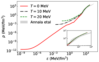
Figure 1: $\beta$-equalibriated eos for various temperatures with rmf model. The model parameters are listed in TABLE 1. The crust part of eos is taken from the Hempel eos by satisfying the thermodynamics of the system.

In FIG. 2 (left), we present the variation of the square of the speed of sound as a function of baryon number density at different temperatures. The speed of sound is higher at high temperatures in low-density regions and remains flatter, while it remains similar across different temperatures in higher densities. This manifests that, for lower densities, the eos for higher temperature is stiffer (for the same energy density, the pressure is higher) than that of low temperature. It may further be observed that the eoss at various temperatures are subluminal and do not violate causality. In FIG. 2 (right), we show the particle fractions as a function of total baryon density at various temperatures, $T=0,\ 10,\ 20\ {\rm MeV}$ for charge-neutral $npe$ matter. Since we are considering only $npe$ matter, the number density of $p$ and $e$ is the same as shown in the figure. We see that as temperature comes into play, it alters the behaviour of the fraction at low densities. The zero temperature effects on the particle fractions have a similar signature as obtained previously [40]. We see that at high temperatures, the fraction of charged ($p$ and $e$) matter is significantly higher than in small temperatures. One reason for this signature is that the temperature induces the inverse $\beta$ decay processes, i.e. $n\to p+e+\bar{\nu}_{e}$.

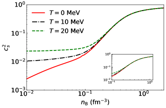
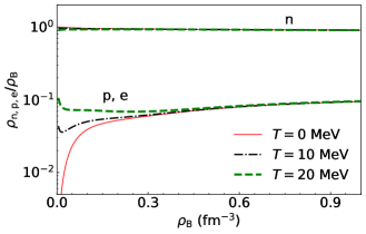
Figure 2: $\beta$-equalibriated eos and square of the speed of sound (right) for different temperatures with rmf model. The model parameters are listed in TABLE 1. The crust part of eos is taken from the Hempel eos.

Once the EoS is obtained, we employ them to obtain the mass-radius curve for NSs. This is done by solving the TOV equation. We employ a few other zero and finite temperature EoS to compare our results with previous works as defined in Table 2. We choose those EoS which are consistent with the present astrophysical bound at zero temperature. We mainly use the NICER and GW170817 bounds [64, 65, 66, 67, 68] and ensure that all EoS can generate at least 2 solar mass stars. This is shown in the left panel of fig 3. At $T=0\ {\rm MeV}$, the eoss produce nss which are consistent with the experimental observations like gw, and, nicer etc. In that, we also show the observation contours; the dark grey shaded region in the figure shows the gw observation while the light green, light yellow and light blue shaded regions in the figure show the nicer observations Miller et al. [65], Riley et al. [67] and Riley et al -2 [68] respectively.

As the temperature of nss decreases, the star becomes more compact as compared with the same mass ns which has a high temperature. The red solid thick curve shows the mass-radius solution of tov equations for a given eos, Eq (II, and II) at $T=0$ while blue dot-dashed (dashed) thick curve shows the mass-radius solution at higher temperature i.e. $T=10\ (20)\ {\rm MeV}$. The other curves in the figure correspond to the solutions corresponding to the different eoss collected in the TABLE 2. Here, as the star cools down, it becomes more compact because the pressure from the thermal part of the eos decreases.

In FIG. 3 (right) we show the non-radial $f$-mode oscillation frequencies of different mass nss corresponding to different eoss (TABLE 2). The red solid thick curve corresponds to the cold (zero temperature) nss while the blue dashed curve corresponds to the hot ($T=20\ {\rm MeV}$) nss. As the temperature of ns decreases, the $f$-mode oscillation frequency increases. The $f$-mode oscillation has no node inside the star and is directly correlated with the mass-radius relation. The f-mode frequency differs considerably for low-mass stars; however, it is very similar for massive stars, irrespective of the temperature. Therefore, for relatively low-mass stars, the detection probability increases with temperature. From this study, it is clear that the observation of non-radial oscillation frequency of hotter ns is less challenging since for the same mass nss, the $f$ mode oscillation frequency is small for hotter ns as compared with colder one. Similar results for the non-radial oscillation frequencies of proto-neutron stars have been found in recent studies [38]. The frequency range for all eoss is consistent with the known range of $f$-mode frequencies ($\sim$ 1 kHz to 3 kHz). The frequencies explicitly depend on the speed of sound (see Eq. III) inversely and are reflected in the figure as well.

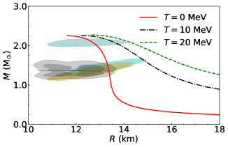
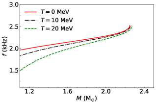
Figure 3: The mass-radius relationships for various $\beta$-equilibrated equations of state (EOS) are illustrated on the left panel, while the right panel depicts the non-radial oscillation $f$-mode frequencies (linear frequencies $f$) as a function of mass for different ns at various temperatures (proton-neutron stars), corresponding to the relativistic mean field (RMF) model EOS (illustrated in FIG. 1).

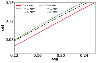
Figure 4: The temperature-dependent universal relations for different equations of state (EoSs) are illustrated in the plot where $\omega$ is the angular frequency ($\omega=2\pi f$). The plot demonstrates that as the temperature increases, the universal relations for different EoSs diverge, with the lines corresponding to these relations shifting upwards (indicating changes in both the x and y intercepts). The slope and intercept of the linear fit are temperature-dependent for nss as shown in FIG 5.

FIG. 4 shows the ur, considering a number of eoss collected in TABLE 2, for different temperatures starting from $T=0\ {\rm MeV}$ to $T=20\ {\rm MeV}$. Several UR are present in the literature, and many are interconnected. In this work, we take the definition of ur as $\omega M=a\left(\frac{M}{R}\right)+b$. The ur for zero temperature is consistent with the results discussed previously [3] showing a small deviation. As temperature increases, the UR shifts towards larger $\omega M$; however, the shift is not linear. It is not easy to understand how the UR behave as temperature increases; therefore, we check how the UR behave by parametrizing it with parameters which depend on temperature. Defining the dimensionless coefficients $a$ and $b$ as temperature-dependent parameters, i.e. $a\equiv a(T)$ and $b\equiv b(T)$. The ur can be recast as

$$\halign to=0.0pt{\relax\global\advance\@IEEEeqncolcnt by 1\relax\begingroup\csname @IEEEeqnarraycolPREr\endcsname#\relax\relax\relax\relax\relax\relax\relax\relax\relax\relax\csname @IEEEeqnarraycolPOSTr\endcsname\relax\relax\relax\relax\relax\relax\relax\relax\relax\relax\endgroup&\relax\global\advance\@IEEEeqncolcnt by 1\relax\begingroup\csname @IEEEeqnarraycolPREC\endcsname#\relax\relax\relax\relax\relax\relax\relax\relax\relax\relax\csname @IEEEeqnarraycolPOSTC\endcsname\relax\relax\relax\relax\relax\relax\relax\relax\relax\relax\endgroup&\relax\global\advance\@IEEEeqncolcnt by 1\relax\begingroup\csname @IEEEeqnarraycolPREl\endcsname#\relax\relax\relax\relax\relax\relax\relax\relax\relax\relax\csname @IEEEeqnarraycolPOSTl\endcsname\relax\relax\relax\relax\relax\relax\relax\relax\relax\relax\endgroup&\global\advance\@IEEEeqncolcnt by 1\relax\bgroup#\egroup&\global\advance\@IEEEeqncolcnt by 1\relax\hbox to\z@\bgroup\hss#\egroup\cr\hfil$\displaystyle\omega M $&\hfil$\displaystyle{}={}$\hfil&$\displaystyle a(T) \left(\frac{M}{R}\right) + b(T) $\hfil&{\vrule width=0.0pt,height=0.0pt,depth=0.0pt}&0.0pt{\hss(28)}\cr}$$

where $a(T)$ and $b(T)$ are defines as

$$\halign to=0.0pt{\relax\global\advance\@IEEEeqncolcnt by 1\relax\begingroup\csname @IEEEeqnarraycolPREr\endcsname#\relax\relax\relax\relax\relax\relax\relax\relax\relax\relax\csname @IEEEeqnarraycolPOSTr\endcsname\relax\relax\relax\relax\relax\relax\relax\relax\relax\relax\endgroup&\relax\global\advance\@IEEEeqncolcnt by 1\relax\begingroup\csname @IEEEeqnarraycolPREC\endcsname#\relax\relax\relax\relax\relax\relax\relax\relax\relax\relax\csname @IEEEeqnarraycolPOSTC\endcsname\relax\relax\relax\relax\relax\relax\relax\relax\relax\relax\endgroup&\relax\global\advance\@IEEEeqncolcnt by 1\relax\begingroup\csname @IEEEeqnarraycolPREl\endcsname#\relax\relax\relax\relax\relax\relax\relax\relax\relax\relax\csname @IEEEeqnarraycolPOSTl\endcsname\relax\relax\relax\relax\relax\relax\relax\relax\relax\relax\endgroup&\global\advance\@IEEEeqncolcnt by 1\relax\bgroup#\egroup&\global\advance\@IEEEeqncolcnt by 1\relax\hbox to\z@\bgroup\hss#\egroup\cr\hfil$\displaystyle a(T) $&\hfil$\displaystyle{}={}$\hfil&$\displaystyle a_{0} + a_{1} T + a_{2} T^{2} $\hfil&{{}\vrule width=0.0pt,height=0.0pt,depth=0.0pt}&0.0pt{\hss(29)}\cr\penalty 100\vskip 3.0pt\vskip 0.0pt\cr\hfil$\displaystyle b(T) $&\hfil$\displaystyle{}={}$\hfil&$\displaystyle b_{0} + b_{1} T + b_{2} T^{2} $\hfil&{\vrule width=0.0pt,height=0.0pt,depth=0.0pt}&0.0pt{\hss(30)}\cr}$$

The values of the parameters are given in Table 3. It is instructive to check how the parameters vary with temperature, and therefore, we plot Fig 5. In FIG 5 (left), we see that the coefficient (slope parameter of the ur, Eq (IV)) $a(T)$ has the parabolic form in temperature. It has a minimum at $T=9\ {\rm MeV}$. The slope of this relation, Eq (IV), is negative for $T<9\ {\rm MeV}$ while positive for $T>9\ {\rm MeV}$. This means that the generalized universal relation oscillates around the minima. The coefficient $b(T)$ starts with a negative value, increases non-linearly with temperature and attains maxima at higher temperatures. Therefore, as both the parameters follow a non-linear behaviour with temperature, the UR shows anomalous behaviour with temperature.

Table 3: The coefficients of urs, Eqs. (IV and IV)

Parameters	Numerical Value
$a_{0}$	$0.65257\pm 8.7\times 10^{-6}$
$a_{1}$	$-0.00284\pm 0.00018\ {\rm MeV}^{-1}$
$a_{2}$	$0.00016\pm 0.00078\ {\rm MeV}^{-2}$
$b_{0}$	$-0.01266\pm 4.09\times 10^{-6}$
$b_{1}$	$0.00155\pm 8.47\times 10^{-5}\ {\rm MeV}^{-1}$
$b_{2}$	$-0.00003\pm 0.00037\ {\rm MeV}^{-2}$

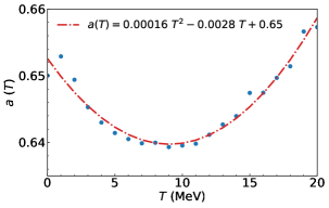
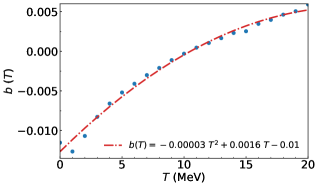
Figure 5: The slope (left) and intercept (right) of the linear fit between $\omega M$ and $\frac{M}{R}$ as a function of temperatures.

V Summary and conclusion

In this study, we investigate the impact of temperature on various properties of nss, specifically focusing on the mass-radius (M-R) relation, the fundamental mode (f-mode) frequency, and universal relations (UR). The temperature influences the eos of the star, which in turn affects these NS properties. Our analysis considers simple $npe$ nuclear matter, and we have developed a relativistic mean field (RMF) model where the coupling is density-dependent, aligning with nuclear saturation properties. The set of equations used ensures that the resulting neutron stars adhere to astrophysical observations for cold nss. It is also assumed that temperature does not directly affect the oscillation equations.

Our findings indicate that temperature predominantly affects the low-density regions of the matter, with minimal impact at higher densities, resulting in negligible variation in the maximum mass with changing temperature. As temperature increases, low-density matter becomes stiffer, leading to a flatter mass-radius curve (i.e., larger radii for the same mass). Consequently, in mass-radius sequences derived from temperature-dependent eoss, low-mass stars, which correspond to lower central energy densities, exhibit significantly larger radii as the temperature rises.

The alterations in the eos and the corresponding changes in the speed of sound significantly influence the f-mode frequency, causing it to shift towards lower values with increasing temperature. This suggests that f-mode frequencies for proto-neutron stars are more easily detectable with gravitational wave detectors. Additionally, we have explored the generalized urs in terms of non-radial oscillation f-mode frequency, radius, and mass of neutron stars. The ur relation demonstrates a nonlinear behaviour with temperature, and when parameterized, the parameters exhibit an oscillatory pattern. This oscillation is primarily due to the temperature effect on the eos, with low-density matter being more affected than high-density matter, causing the lower region of the universal relation to align across various temperatures. This nonlinearity is also evident in the mass-radius sequence, where for the same mass, a higher radius is observed (corresponding to lower energy densities) as temperature increases.

Our current analysis assumes temperature only affects the eos without explicitly influencing the hydrostatic equilibrium condition and the perturbation equations that give rise to oscillation modes. However, this assumption may not be accurate, as temperature could significantly affect these aspects. Investigating these potential influences is a priority for our immediate future research.

VI Acknowledgement

DK and RM would like to acknowledge the financial support from the Science and Engineering Research Board under the project no. CRG/2022/000663, India.

Appendix A Extra plots:

Figures showing the comparisons of other EoS for the mass-radius, f-mode frequency and UR.

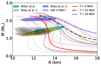
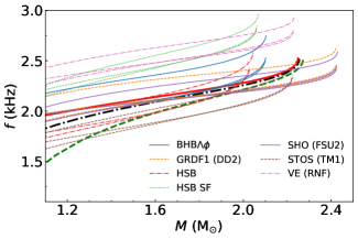
Figure 6: The mass-radius relationships for various $\beta$-equilibrated eoss are illustrated on the left panel, while the right panel depicts the non-radial oscillation $f$-mode frequencies (linear frequencies $f$) as a function of mass for different ns at various temperatures (proton-neutron stars), corresponding to the different models collected in table 2 along with our eos (illustrated in FIG. 1).

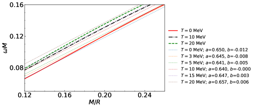
Figure 7: The temperature-dependent universal relations for different eoss are illustrated in the plot where $\omega$ being angular frequency ($\omega=2\pi f$). The plot demonstrates that as the temperature increases, the universal relations for different eoss diverge, with the lines corresponding to these relations shifting upwards (indicating changes in both the x and y intercepts). The slope and intercept of the linear fit are temperature-dependent for nss as shown in FIG 5.

References

- [1] M. G. Alford, S. Han, and K. Schwenzer, “Signatures for quark matter from multi-messenger observations,” J. Phys. G, vol. 46, no. 11, p. 114001, 2019.
- [2] J. P. Pereira, M. Bejger, L. Tonetto, G. Lugones, P. Haensel, J. L. Zdunik, and M. Sieniawska, “Probing elastic quark phases in hybrid stars with radius measurements,” Astrophys. J., vol. 910, no. 2, p. 145, 2021.
- [3] D. Kumar, H. Mishra, and T. Malik, “Non-radial oscillation modes in hybrid stars: consequences of a mixed phase,” JCAP, vol. 02, p. 015, 2023.
- [4] M. Mannarelli, K. Rajagopal, and R. Sharma, “Testing the Ginzburg-Landau approximation for three-flavor crystalline color superconductivity,” Phys. Rev. D, vol. 73, p. 114012, 2006.
- [5] K. Rajagopal and R. Sharma, “The Crystallography of Three-Flavor Quark Matter,” Phys. Rev. D, vol. 74, p. 094019, 2006.
- [6] K. N. Singh, A. Banerjee, S. K. Maurya, F. Rahaman, and A. Pradhan, “Color-flavor locked quark stars in energy–momentum squared gravity,” Phys. Dark Univ., vol. 31, p. 100774, 2021.
- [7] M. G. Alford, K. Rajagopal, and F. Wilczek, “Color flavor locking and chiral symmetry breaking in high density QCD,” Nucl. Phys. B, vol. 537, pp. 443–458, 1999.
- [8] Z. Roupas, G. Panotopoulos, and I. Lopes, “QCD color superconductivity in compact stars: color-flavor locked quark star candidate for the gravitational-wave signal GW190814,” Phys. Rev. D, vol. 103, no. 8, p. 083015, 2021.
- [9] P.-C. Chu, H. Liu, X.-H. Li, M. Ju, X.-H. Wu, and X.-M. Zhang, “Quark star matter in the color-flavor-locked state with a density-dependent quark mass model,” J. Phys. G, vol. 51, no. 6, p. 065202, 2024.
- [10] A. Kurkela, K. Rajagopal, and R. Steinhorst, “Astrophysical Equation-of-State Constraints on the Color-Superconducting Gap,” 1 2024.
- [11] H. Mishra, “Colorsuperconductivity in magnetised quark matter: an NJL model approach,” Eur. Phys. J. ST, vol. 231, no. 2, pp. 103–127, 2022.
- [12] A. Abhishek and H. Mishra, “Chiral symmetry breaking, color superconductivity, and equation of state for magnetized strange quark matter,” Phys. Rev. D, vol. 99, no. 5, p. 054016, 2019.
- [13] M. Mannarelli, “Overview of Crystalline Color Superconductors,” in Compact Stars in the QCD Phase Diagram IV, 5 2015.
- [14] S. Pal and G. Chaudhuri, “Effect of dark matter interaction on hybrid star in the light of the recent astrophysical observations,” 5 2024.
- [15] M. F. Barbat, J. Schaffner-Bielich, and L. Tolos, “A comprehensive study of compact stars with dark matter,” 4 2024.
- [16] C.-T. Lu, A. K. Mishra, and L. Wu, “Constraining Bosonic Dark Matter-Baryon Interactions from Neutron Star Collapse,” 4 2024.
- [17] T. Fischer, M.-R. Wu, B. Wehmeyer, N.-U. F. Bastian, G. Martínez-Pinedo, and F.-K. Thielemann, “Core-collapse Supernova Explosions Driven by the Hadron-quark Phase Transition as a Rare -process Site,” Astrophys. J., vol. 894, no. 1, p. 9, 2020.
- [18] J. A. Pons, S. Reddy, M. Prakash, J. M. Lattimer, and J. A. Miralles, “Evolution of Proto-Neutron Stars,” Astrophys. J. , vol. 513, pp. 780–804, Mar. 1999.
- [19] A. Burrows and J. M. Lattimer, “The Birth of Neutron Stars,” Astrophys. J. , vol. 307, p. 178, Aug. 1986.
- [20] R. Negreiros, R. Ruffini, C. L. Bianco, and J. A. Rueda, “Cooling of young neutron stars in GRB associated to Supernova,” Astron. Astrophys., vol. 540, p. A12, 2012.
- [21] D. G. Yakovlev and C. J. Pethick, “Neutron star cooling,” Ann. Rev. Astron. Astrophys., vol. 42, pp. 169–210, 2004.
- [22] J. P. Cox, Theory of Stellar Pulsation. (PSA-2), Volume 2, vol. 2. 1980.
- [23] K. D. Kokkotas and B. G. Schmidt, “Quasi-normal modes of stars and black holes,” Living Reviews in Relativity, vol. 2, Sept. 1999.
- [24] J. Arponen, “Internal structure of neutron stars,” Nucl. Phys. A, vol. 191, pp. 257–282, 1972.
- [25] A. Reisenegger and P. Goldreich, “Excitation of Neutron Star Normal Modes during Binary Inspiral,” Astrophys. J. , vol. 426, p. 688, May 1994.
- [26] N. K. Glendenning, Compact stars: Nuclear physics, particle physics, and general relativity. 1997.
- [27] B. K. Pradhan, D. Chatterjee, M. Lanoye, and P. Jaikumar, “General relativistic treatment of -mode oscillations of hyperonic stars,” 3 2022.
- [28] J. Nättilä, A. W. Steiner, J. J. E. Kajava, V. F. Suleimanov, and J. Poutanen, “Equation of state constraints for the cold dense matter inside neutron stars using the cooling tail method,” Astron. Astrophys., vol. 591, p. A25, 2016.
- [29] F. Özel and P. Freire, “Masses, Radii, and the Equation of State of Neutron Stars,” Ann. Rev. Astron. Astrophys., vol. 54, pp. 401–440, 2016.
- [30] A. W. Steiner, J. M. Lattimer, and E. F. Brown, “The Equation of State from Observed Masses and Radii of Neutron Stars,” Astrophys. J., vol. 722, pp. 33–54, 2010.
- [31] A. L. Watts et al., “Colloquium : Measuring the neutron star equation of state using x-ray timing,” Rev. Mod. Phys., vol. 88, no. 2, p. 021001, 2016.
- [32] N. Andersson and K. D. Kokkotas, “Gravitational waves and pulsating stars: What can we learn from future observations?,” Phys. Rev. Lett., vol. 77, pp. 4134–4137, 1996.
- [33] A. Torres-Forné, P. Cerdá-Durán, A. Passamonti, and J. A. Font, “Towards asteroseismology of core-collapse supernovae with gravitational-wave observations – I. Cowling approximation,” Mon. Not. Roy. Astron. Soc., vol. 474, no. 4, pp. 5272–5286, 2018.
- [34] A. Torres-Forné, P. Cerdá-Durán, A. Passamonti, M. Obergaulinger, and J. A. Font, “Towards asteroseismology of core-collapse supernovae with gravitational wave observations – II. Inclusion of space–time perturbations,” Mon. Not. Roy. Astron. Soc., vol. 482, no. 3, pp. 3967–3988, 2019.
- [35] Y. Ashida, “Multi-energy diffuse neutrino fluxes originating from core-collapse supernovae,” 1 2024.
- [36] M. Cavan-Piton, D. Guadagnoli, M. Oertel, H. Seong, and L. Vittorio, “Axion emission from strange matter in core-collapse SNe,” 1 2024.
- [37] H.-S. Wang and K.-C. Pan, “The Influence of Stellar Rotation in Binary Systems on Core-Collapse Supernova Progenitors and Multi-messenger Signals,” 1 2024.
- [38] N. Lozano, V. Tran, and P. Jaikumar, “Temperature Effects on Core g-Modes of Neutron Stars,” Galaxies, vol. 10, no. 4, p. 79, 2022.
- [39] S. Typel, G. Ropke, T. Klahn, D. Blaschke, and H. H. Wolter, “Composition and thermodynamics of nuclear matter with light clusters,” Phys. Rev. C, vol. 81, p. 015803, 2010.
- [40] A. Mishra, P. K. Panda, and W. Greiner, “Vacuum polarization effects in hyperon rich dense matter: A Nonperturbative treatment,” J. Phys. G, vol. 28, pp. 67–83, 2002.
- [41] L. Tolos, M. Centelles, and A. Ramos, “Equation of State for Nucleonic and Hyperonic Neutron Stars with Mass and Radius Constraints,” Astrophys. J., vol. 834, no. 1, p. 3, 2017.
- [42] S. Typel, “Relativistic Mean-Field Models with Different Parametrizations of Density Dependent Couplings,” Particles, vol. 1, no. 1, pp. 3–22, 2018.
- [43] S. Typel and H. H. Wolter, “Relativistic mean field calculations with density dependent meson nucleon coupling,” Nucl. Phys. A, vol. 656, pp. 331–364, 1999.
- [44] T. Malik, S. Banik, and D. Bandyopadhyay, “Equation-of-state Table with Hyperon and Antikaon for Supernova and Neutron Star Merger,” Astrophys. J., vol. 910, no. 2, p. 96, 2021.
- [45] T. Malik, M. Ferreira, B. K. Agrawal, and C. Providência, “Relativistic description of dense matter equation of state and compatibility with neutron star observables: a Bayesian approach,” 1 2022.
- [46] T. Malik, B. K. Agrawal, and C. Providência, “Inferring the nuclear symmetry energy at suprasaturation density from neutrino cooling,” Phys. Rev. C, vol. 106, no. 4, p. L042801, 2022.
- [47] S. Banik, M. Hempel, and D. Bandyopadhyay, “New Hyperon Equations of State for Supernovae and Neutron Stars in Density-dependent Hadron Field Theory,” Astrophys. J. Suppl., vol. 214, no. 2, p. 22, 2014.
- [48] P. Möller, M. R. Mumpower, T. Kawano, and W. D. Myers, “Nuclear properties for astrophysical and radioactive-ion-beam applications (II),” Atom. Data Nucl. Data Tabl., vol. 125, pp. 1–192, 2019.
- [49] P. Moller, J. R. Nix, and K. L. Kratz, “NUCLEAR PROPERTIES FOR ASTROPHYSICAL AND RADIOACTIVE-ION-BEAM APPLICATIONS,” Atom. Data Nucl. Data Tabl., vol. 66, pp. 131–343, 1997.
- [50] M. Hempel and J. Schaffner-Bielich, “Statistical Model for a Complete Supernova Equation of State,” Nucl. Phys. A, vol. 837, pp. 210–254, 2010.
- [51] S. Typel, “Equations of state for astrophysical simulations from generalized relativistic density functionals,” J. Phys. G, vol. 45, no. 11, p. 114001, 2018.
- [52] H. Pais and S. Typel, COMPARISON OF EQUATION OF STATE MODELS WITH DIFFERENT CLUSTER DISSOLUTION MECHANISMS, ch. CHAPTER 4, pp. 95–132.
- [53] S. Typel, H. H. Wolter, G. Röpke, and D. Blaschke, “Effects of the liquid-gas phase transition and cluster formation on the symmetry energy,” Eur. Phys. J. A, vol. 50, p. 17, 2014.
- [54] H. Toki, D. Hirata, Y. Sugahara, K. Sumiyoshi, and I. Tanihata, “Relativistic many body approach for unstable nuclei and supernova,” Nuclear Physics A, vol. 588, no. 1, pp. c357–c363, 1995. Proceedings of the Fifth International Symposium on Physics of Unstable Nuclei.
- [55] L. Geng, H. Toki, and J. Meng, “Masses, Deformations, and Charge Radii–Nuclear Ground-State Properties in the Relativistic Mean Field Model,” Progress of Theoretical Physics, vol. 113, pp. 785–800, Apr. 2005.
- [56] M. Hempel, T. Fischer, J. Schaffner-Bielich, and M. Liebendorfer, “New Equations of State in Simulations of Core-Collapse Supernovae,” Astrophys. J., vol. 748, p. 70, 2012.
- [57] P. Möller, J. R. Nix, and K. L. Kratz, “Nuclear Properties for Astrophysical and Radioactive-Ion Beam Applications,” Atomic Data and Nuclear Data Tables, vol. 66, p. 131, Jan. 1997.
- [58] A. W. Steiner, M. Hempel, and T. Fischer, “Core-collapse supernova equations of state based on neutron star observations,” Astrophys. J., vol. 774, p. 17, 2013.
- [59] H. Togashi, K. Nakazato, Y. Takehara, S. Yamamuro, H. Suzuki, and M. Takano, “Nuclear equation of state for core-collapse supernova simulations with realistic nuclear forces,” Nucl. Phys. A, vol. 961, pp. 78–105, 2017.
- [60] H. Shen, H. Toki, K. Oyamatsu, and K. Sumiyoshi, “Relativistic equation of state of nuclear matter for supernova and neutron star,” Nucl. Phys. A, vol. 637, pp. 435–450, 1998.
- [61] Z. Guo, “Asteroseismology of close binary stars: Tides and mass transfer,” Frontiers in Astronomy and Space Sciences, vol. 8, p. 663026, 05 2021.
- [62] H. Sotani, N. Yasutake, T. Maruyama, and T. Tatsumi, “Signatures of hadron-quark mixed phase in gravitational waves,” Phys. Rev. D, vol. 83, p. 024014, 2011.
- [63] E. Annala, T. Gorda, A. Kurkela, and A. Vuorinen, “Gravitational-wave constraints on the neutron-star-matter Equation of State,” Phys. Rev. Lett., vol. 120, no. 17, p. 172703, 2018.
- [64] B. P. Abbott et al., “Properties of the binary neutron star merger GW170817,” Phys. Rev. X, vol. 9, no. 1, p. 011001, 2019.
- [65] M. C. Miller et al., “PSR J0030+0451 Mass and Radius from Data and Implications for the Properties of Neutron Star Matter,” Astrophys. J. Lett., vol. 887, no. 1, p. L24, 2019.
- [66] M. C. Miller et al., “The Radius of PSR J0740+6620 from NICER and XMM-Newton Data,” Astrophys. J. Lett., vol. 918, no. 2, p. L28, 2021.
- [67] T. E. Riley et al., “A View of PSR J0030+0451: Millisecond Pulsar Parameter Estimation,” Astrophys. J. Lett., vol. 887, no. 1, p. L21, 2019.
- [68] T. E. Riley et al., “A NICER View of the Massive Pulsar PSR J0740+6620 Informed by Radio Timing and XMM-Newton Spectroscopy,” Astrophys. J. Lett., vol. 918, no. 2, p. L27, 2021.